Towards the Equation of State of Classical SU(2) Lattice

Gauge Theory

Á. Fülöp, T. S. Biró

RMKI, KFKI

H-1525 Budapest, P.O. Box 49, Hungary

Abstract

We determine numerically the full complex Lyapunov spectrum of SU(2) Yang-Mills fields on a 3-dimensional lattice from the classical chaotic dynamics using eigenvalues of the monodromy matrix. The microcanonical equation of state is determined as the entropy – energy relation utilizing the Kolmogorov-Sinai entropy extrapolated to the large size limit.

Introduction

Knowledge of the microscopic mechanism responsible for the local equilibration of energy and momentum in the nuclear collision is fundamental to understand the possible emergence of a quark gluon plasma in relativistic heavy-ion collisions. It is evenly essential to study the equation of state of this system (in and out of equilibrium) in order to be able to make predictions or interpret experimental data from the perspective of quark – gluon matter.

Many of the approaches to the equation of state assume thermal equilibrium, since the real – time evolution of such a plasma in the full quantum field theory cannot yet be followed in a non-perturbative manner by presently practized numerical methods. Perturbative QCD helps to get hints from the high-energy parton dynamics, but the non-perturbative lattice gauge theory is difficult to extend to non-equilibrium phenomena.

Fortunately, the situation is eased by findings which point to the possibility that the quark – gluon plasma can be dynamically studied in a semiclassical approximation. Hard thermal loop resummation has been shown to cope with the semiclassical transport (linear response) theory approach [2, 3]. In fact earlier numerical studies of the classical Hamiltonian dynamics of Yang-Mills systems on three – dimensional lattices revealed an intriguing coincidence between the maximal Lyapunov exponent and twice the gluon damping rate [4]. In the background of that argumentation equipartition of the energy has been conjectured as a result of the classical chaotic dynamics on the lattice. This conjecture has been supported by the pseudo – Boltzmannian distribution of one-plaquette energies (the local magnetic energy density) in long-evolved classical configurations.

The correspondence between this average energy and the Kolmogorov-Sinai entropy has been first investigated in [5] for pure SU(2) Yang-Mills systems. Those times, however, the Lyapunov spectrum could be obtained only for relatively small systems (N=2,3) with the rescaling method. This way also only the positive real exponents could have been calculated. The question of the thermodynamical limit ($N\longrightarrow\infty$) and the investigation of a possible dependence on the initial configuration (which is usually done by using improved statistics) remained open. (Citation: “Future work is still required here” [[5], page 6].)

In the present article we study the ergodization of SU(2) lattice gauge theory due to its classical chaotic dynamics by using different methods as before. We also consider larger lattices ($N=2,3,4,5,6$) for obtaining the entropy and extrapolate to the large $N$ limit. In our approach the full complex spectrum of Lyapunov exponents will be obtained using the monodromy matrix (linear stability matrix along the path determined by the classical equation of motion) in the space of evolving field configurations on the lattice. The complex spectrum offers an insight also into the periodic (oscillatory) behavior of field fluctuations; a basic experience for learning about the corresponding quantum theory.

The question of ergodization is addressed via the Kolmogorov-Sinai entropy, which is calculated up to linear lattice sizes of $N=6$ (using $24N^{3}=5184$ dimensional phase-space) and extrapolated to $N\longrightarrow\infty$. We extrapolate both for long times, – in order to get close to the Lyapunov exponents, – and for large systems – in order to approach the thermodynamical limit. Ensembles of randomly chosen (i.e. chosen according to the Haar measure in the group variables) initial configurations with a given (slightly fluctuating) total energy are averaged over, too.

This article is constructed as follows. First we review basic definitions dealing with the chaotic behavior of extended systems and then the Hamiltonian treatment of classical lattice gauge theory. Finally we present results on full complex Lyapunov spectra, scaling properties, extrapolations and the entropy - energy relation (microcanonical equation of state) for SU(2) lattice gauge theory.

Measuring Chaos

Instead of the classical determination of the Lyapunov exponent, which has been calculated by the rescaling method in [5, 6, 7, 8, 9], in this article we use the monodromy matrix approach. The Lyapunov spectrum $L_{i}$ is expressed in terms of the monodromy matrix’s eigenvalues $\Lambda_{i}$:

$$L_{i}=\lim_{T\rightarrow\infty}\frac{\int_{0}^{T}\Lambda_{i}(t)dt}{T}\;\;\;\;\;\;\;i=1....f$$ (1)

where the $\Lambda_{i}(t)$-s are the solutions of the characteristic equation

$${\rm det}\left(\Lambda_{i}(t)1-M(t)\right)=0$$ (2)

at a given time $t$. Here $M$ is the linear stability matrix, $f$ is the number of degrees of freedom.

We consider conservative dynamics fulfilling Liouville’s theorem.

$$\sum_{i=0}^{f}L_{i}=0$$ (3)

In the numerical calculation we use the discrete definition of the Lyapunov spectrum:

$$L_{i}^{{}^{\prime}}=\left<\Lambda_{i}\right>^{(n)}=\frac{1}{n}\sum_{j=1}^{n}\Lambda_{i}(t_{j-1})\\ i=1...f,$$ (4)

where $t_{j}$ are subsequent times along an evolutionary path of the gauge field configurations. Nevertheless a few initial configurations has been omitted from the average, although the starting configurations has been produced randomly. We need to extrapolate the quantities $L_{i}^{{}^{\prime}}$ to the long time limit $n\rightarrow\infty,$ with fixed timestep. It is expected to converge to Lyapunov exponent $L_{i}$ occuring in eq. (1) for a non-compact configuration space. As we shall see by discussing the results of numerical simulations gauge group systems live in a compact configuration space, therefore this limit is not entirely safe in our case. The rescaling method observes pairs of gauge field configurations which are close in the phase space, so it has a control on the distance of these two and can monitor this quantity not growing close to or over the limiting distance given by the compact size of the phase space. It is achieved by doing frequent rescalings. The monodromy matrix method on the other hand follows only one gauge field evolution, in this case the short and long time behavior can be different.

The Kolmogorov-Sinai entropy is obtained by using Perin’s formula:

$$h^{KS}=\sum_{i}L_{i}\Theta(L_{i})$$ (5)

using the theta function $\Theta(x)$ being one for positive arguments and zero otherwide. The dimension of $h^{KS}$ yet is a rate (1/time), so for estimating the entropy we shall use the normalized quantity:

$$S=\frac{h^{KS}}{Re(L_{0})N^{3}}.$$ (6)

The redefinition is done in a way typical for extensive quantities, here the entropy density, on an $N\times N\times N$ lattice.

Lattice Yang-Mills field systems

Our discussion is based on the Hamiltonian formulation of the classical lattice SU(2) gauge theory. It is governed by the Hamiltonian [10]:

$$H=\sum_{x,i}\left(\frac{1}{2}\left<\dot{U}_{x,i},\dot{U}_{x,i}\right>+\left(1-\frac{1}{4}\left<U_{x,i},V_{x,i}\right>\right)\right)$$ (7)

where $U_{x,i}$ is the SU(2) group element lying on an oriented link of the lattice starting at the site x, pointing to the i direction. In the numerical realization it is represented by real quaternions. The notation $<A,B>$ belongs to the normalized trace of the product of two SU(2) group elements :

$$<A,B>=\frac{1}{2}tr(AB^{-1}).$$ (8)

The $V_{x,i}$ complement matrix is constructed from triple products of link variables, which complete the considered link (x,i) to an elementary plaquette.

$$V_{x,i}=\frac{1}{4}\sum_{i,j,k}U_{i}U_{j}^{-1}U_{k}^{-1}$$ (9)

Finally the overdots denote the derivative with respect to the scaled time, $t/a$, as well as the Hamiltonian $H$ stands for the scaled energy $g^{2}aE$.

The Hamiltonian equations of motions are given by (suppressing the link indices in the rotation):

$$\dot{U} = P,$$

$$\dot{P} = V-\left<U,V\right>U-\left<P,P\right>U.$$ (10)

These equations of motion conserve unitarity $<U,U>=1$ , orthogonality $<U,P>=0$, and Gauss’ law. The monodromy matrix is defined as:

$$M=\left(\begin{array}[]{cc}\frac{\partial\dot{U}}{\partial U}&\frac{\partial\dot{U}}{\partial P}\\ \\ \frac{\partial\dot{P}}{\partial U}&\frac{\partial\dot{P}}{\partial P}\\ \end{array}\right)$$ (11)

Here the different partial derivatives are obtained by comparing the above equations of motion for the configurations $(U,P)$ and $(U+\delta U,P+\delta P).$ We arrive at

$$\frac{\partial\dot{U}^{a}}{\partial U^{b}} = 0,$$

$$\frac{\partial\dot{U}^{a}}{\partial P^{b}} = \delta^{ab},$$

$$\frac{\partial\dot{P}^{a}}{\partial U^{b}} = \frac{\partial V^{a}}{\partial U^{b}}-\left(U_{c}\frac{\partial V^{c}}{\partial U^{b}}\right)U^{a}-V^{b}U^{a}-(U_{c}V^{c}+P_{c}P^{c})\delta^{ab},$$

$$\frac{\partial\dot{P}^{a}}{\partial P^{b}} = -2P^{b}U^{a}.$$ (12)

These expressions provide information about the stability of trajectories in the neighbourhood of any point of an orbit in the (U,P) phase space. A small perturbation, $(\delta U,\delta P)$ evolves in time governed by the monodromy matrix $M.$ The eigenvalues of this matrix can be classified as follows: for real and positive eigeinvalues neighbouring trajectories apart exponentially and the motion is unstable. In the limit of large time we obtain the Lyapunov exponents from these eigenvalues. The imaginary parts of the complex eigenvalues describe oscillatory frequencies of perturbations.

In contrast to the rescaling method, where only the positive real part of the Lyapunov exponent can be measured, the study of the spectrum of the monodromy matrix makes these complex eigenvalues numerically available for the first time. The total number of degrees of freedom in the numerical simulation is given by $f=4*3*N^{3}=12*N^{3}$, using four-real element quaternions for SU(2) group elements (so the phase space is $2f=24N^{3}$ dimensional). Due to the constrains $<U,U>=1$, however, the physically relevant number of degrees of freedom is the same as in earlier simulations, which used $E^{a}$, and ${\rm tr}(U\tau^{a})$ as independent degrees of freedom.

The spectrum of the stability matrix

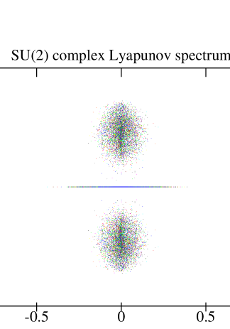
Figure 2: Full eigenvalue spectrum of the monodromy matrix: low energy.

The eigenvalue spectrum $\Lambda_{i}$ of the monodromy matrix consists of a real subset and a complex subset on the complex plane (cf. Figs. 1 and 2). Although this $2f\times 2f$ sized matrix is sparse, since each group element exerts a force onto close links (those sharing a common plaquette) only, the usual sparse matrix methods are not applicable, because they determine just a few leading eigenvalues. In order to determine all complex eigenvalues with an acceptable precision, only ‘brute force’ methods with a memory need of ${\cal O}(f^{2})$ and computational time of ${\cal O}(f^{3})$ can be used. The maximal system size, our computational resources allow us to use, belongs to $N=6,$ meaning a $2f=5904$ dimensional phase space.

Figs.1 and 2 display the complex eigenvalues for several configurations during the evolution along a few trajectories. At high energy per degree of freedom, $g^{2}aE=0.8,$ (near to the saturation value $1$) the region covered by the eigenvalues in the complex plane shows a mirrorred “butterfly” shape, while at low energy, $g^{2}aE=0.1,$ rather two “ovals”. In all cases the covered region is symmetric both to the real and imaginary axes: the former property is due to the fact that the equations of motion are real, the latter is due to the Hamiltonian is conservative (time independent). It is interesting to observe that about one sixth of the eigenvalues are purely real, not allowing for oscillations or wave-propagation in the fluctuations. In neither case shows the eigenvalue region any resemblence of Wigner semicircles, like those found in studies of the eigenvalues of the Dirac operator in random gauge field background [11], and usually regarded as a signature of quantum chaos. Here we deal with a bosonic system at comparatively high excitations and the chaotic behavior is quite classical.

According to the imaginary part of the eigenvalues the pattern separates to three islands at all energies. An important qualitative feature of these patterns is the gap between zero and non-zero imaginary parts: it behaves as a dynamically developed infrared cut-off (“gluon mass”) for oscillations in small perturbations of the classical equations of motion. Also a number of zero-frequency modes occur, this is connected to symmetry transformations commuting (in the Poisson bracket sense) with the Hamiltonian, such as time independent gauge transformations. The gap seems to be reduced and eventually disappear at high energy. Do these differences between low and high energy establish a two-phase picture of the classical lattice SU(2) system? In order to answer this question a study of the equation of state is necessary.

Scaling and Equation of State

We aim to obtain the equation of state from the dynamical simulation. For this purpose we first study the finite size scaling and extrapolate to infinite ($1/N=0$) lattices. Then we study the energy dependence of the maximal Lyapunov exponent as well as the Kolmogorov-Sinai entropy. The latter leads eventually to the equation of state as the entropy - energy relation, $S(E),$ in the thermodynamical limit of infinite volume.

Fig.3 shows the real part of the Lyapunov spectrum extrapolated to $1/N\rightarrow 0$ from data taken at $N=2,3,4,5$ and $6$ at high energy ($g^{2}aE=0.8$). The overall pattern is similar to that obtained earlier for smaller systems ($N=2,3$), just the number of purely imaginary eigenvalues (for those ${\rm Re}L_{i}=0$) is greater due to our use of more variables (and, of course, more constraints). The structure of the ordered real part of the Lyapunov spectrum is similar at all energies, but the maximal point, $aL_{0},$ scales with the energy, $g^{2}aE.$

Fig.4 displays the fluctuation of the maximal real part Lyapunov exponent, $L_{0},$ originating in different, randomly chosen initial field configurations. This levels at a few per cent. The energy scaling of the maximal Lyapunov exponent has been debated in the past and has been found linear in the long-time limit. Doubts rose for low energies [12, 13], stating that the correct scaling here would be $L_{0}\sim E^{1/4}.$ More elaborated studies with the rescaling – aparting method showed then a tendency back to the linear, $L_{0}\sim E$ scaling also at low energies for long enough time observations [14, 15, 16]. Our data agree with the linear scaling with a coefficient of $0.5$ for a middle to short time evolution, as it can be seen in Fig.5. Surprisingly, and not yet fully understood, the very long time behavior of the maximal real part of the monodromy matrix eigenvalues show a definitely sublinear scaling with the energy per degree of freedom. The best fit is, however, not like $E^{1/4},$ but rather a logarithm (cf. Fig.6). We suspect that following a trajectory too long makes the observed eigenvalues feel the compactness of the configuration space – which is an artefact of the lattice field theory Hamiltonian. In the following discussion we refer to data with linear energy scaling only.

Fig.7 displays the extrapolation of the maximal Lyapunov exponents to the thermodynamical limit at different energies. The correspondence proved to be almost linear by assuming an

$$L_{0}\sim\frac{1}{\sqrt{f}}\sim N^{-3/2}$$

scaling with the finite size. This corresponds to sampling ergodic states [16]. In particular at high energies the extrapolated $L_{0}$ is higher than any actually obtained value in simulations at the finite $N.$

Finally we obtained the Kolmogorov-Sinai entropy from infinite-size extrapolated, initial state and evolution averaged eigenvalue spectra as a function of the scaled energy. For a (nearly) ideal gas on expects an $S\sim\log E$ relation, indeed this is a good approximation of our data (cf. Fig.8). We obtain

$$\langle S\rangle=(0.5084\pm 0.023)\log(g^{2}aE)\,+\,(2.3334\pm 0.0452).$$ (13)

The indicated errors after the $\pm$ signs are of statistical nature. This best fit belongs to an inverse temperature

$$\frac{1}{T}=\frac{\partial\langle S\rangle}{\partial E}\approx\frac{0.5}{E},$$ (14)

describing equipartion with

$$E=\frac{1}{2}T.$$ (15)

Based upon our calculations even a two-phase structure (or a crossover) cannot be excluded with absolute safety: at mid energies a depletion is hinted in the data. The $S(E)$ curve would show a first order two-phase structure by having a break somewhere. For a possible relevance to lattice SU(2) systems see the paper [17]. In our case, starting from the chaotic dynamics of classical lattice Hamiltonians, a refined study is needed in the transition region $g^{2}aE=0.2,\ldots 0.5$ in order to settle this question.

Acknowledgements

One of us (Á.F.) gratefully acknowledges discussions with professor Tamás Tél. This work has been supported by the Hungarian – American Joint Fund MAKA TéT (JF.Nr. 649).

FIGURES

      

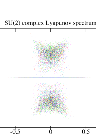
Figure 1: Full complex eigenvalue spectrum of monodromy matrix: high energy.

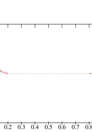
Figure 3: The real part of the Lyapunov spectra in the case of $N\rightarrow\infty$

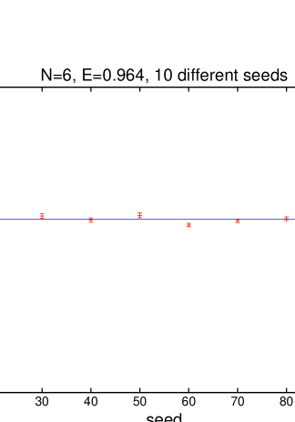
Figure 4: Maximal Lyapunov exponent obtained starting from different random configurations on an $N=6$ lattice at scaled energy $g^{2}aE=0.964$.

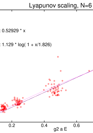
Figure 5: Scaling of short time Lyapunov exponents with energy (before reaching the saturation in the distance of two initially adjacent configurations due to the compactness of the configuration space).

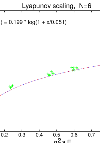
Figure 6: Scaling of Lyapunov exponents with energy for long time evolution of the monodromy matrix (after reaching distance saturation in the compact configuration space).

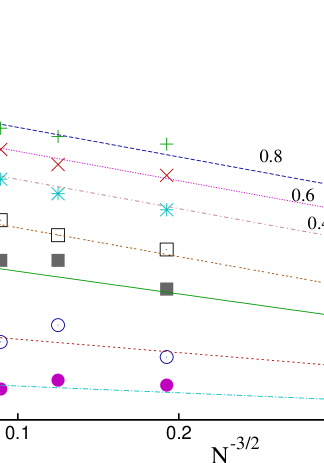
Figure 7: Finite size scaling of the maximal Lyapunov exponent. The straight line fits belong to different scaled energies (marked in the plot).

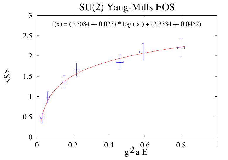
Figure 8: The normalized Kolmogorov-Sinai entropy. The best fit belongs to $\frac{1}{2}kT$ energy per degree of freedom, but a two phase structure also cannot be excluded (depletion hint).

References

- [1]
- [2] J.-P. Blaizot, E. Iancu, A. Rebhan, Approximately self-consitent resummations for the thermodynamics of the quark-gluon plasma.I. Entropy and density, Phys. Rev. D 63:065003, 2001
- [3] J.-P. Blaizot, E. Iancu, A.Rebhan, The entropy of the QCD plasma, Phys. Rev. Lett. 83 (1999) 2906-2909
- [4] T.S. Biró, C. Gong, B. Müller, Lyapunov exponent and plasmon damping rate in non-Abelian gauge theories, Phys. Rev. D 52 (1995) 1260-1266
- [5] C. Gong, Phys. Rev. D 49 (1994) 2642
- [6] B. Müller, A Trayanov, Phys. Rev. Lett 68 (1992) 3387
- [7] C. Gay, Lyapunov exponent of Classical SU(3) Gauge Theory, Phys. Lett. B 298 (1993) 257-262
- [8] T. S. Biró, C. Gong, B. Müller, A. Trayanov, Journal of Modern Physics C, Vol. 5, No. 1.(1994) 113-149
- [9] T.S. Biró, Á. Fülöp, M. Feurstein, H. Markum, Investigation of Chaotic Dynamics of Lattice Gauge Configurations Created by Monte Carlo Techniques, Conference Proceedings, ”Strong and Electroweak Matter ’97” Eger,(1997), in World Scientific Publishing Co., (1997) p.304
- [10] T.S. Biró, S.G. Matinyan, B. Müller, Chaos and Gauge Field Theory, World Scientific 1995.
- [11] H.Markum, R.Pulirsch, T.Wettig, Nonhermitian Random Matrix Theory and Lattice QCD with Chemical Potebtial, Phys.Rev.Lett. 83: 484, 1999
- [12] H.B. Nielsen, H.H. Rugh, S.E. Rugh, Chaos and Scaling in Classical Non-Abelian Gauge Fields, chao-dyn/9606013
- [13] H.B. Nielsen, H.H. Rugh, S.E. Rugh, Chaos, scaling and existence of a continuum limit in classical non-Abelian lattice gauge theory, hep-th/9611128
- [14] B. Müller, Study of Chaos and Scaling in Classical SU(2) Gauge Theory, chao-dyn/9607001
- [15] U. Heinz, C. R. Hu, S. Leupold, S. G. Matinyan, B. Müller, Thermalization and Lyapunov exponens in the Yang-Mills Higgs Theory, Phys. Rev. D 55 (1997) 2464-2476
- [16] J. Bolte, B. Müller, A. Schafer, hep-lat/9906037 Phys.Rev.D 61: 054506, 2000
- [17] D.R. Stump, Entropy of the SU(2) lattice gauge field, Phys. Rev. D 36 (1987) 520-526