Invariant Operators in Collinear Effective Theory

Abstract

We consider processes which produce final state hadrons whose energy is much greater than their mass. In this limit interactions involving collinear fermions and gluons are constrained by a symmetry, and we give a general set of rules for constructing leading and subleading invariant operators. Wilson coefficients $C(\mu,\bar{\cal P})$ are functions of a label operator $\bar{\cal P}$, and do not commute with collinear fields. The symmetry is used to reproduce a two-loop result for factorization in $B\to D\pi$ in a simple way.

I Introduction

For processes involving the production of a highly energetic hadron, $E_{H}\gg m_{H}$, a large number of quarks and gluons typically move close to a light cone direction $n^{\mu}$. The QCD dynamics of these collinear particles is easiest to describe with light cone coordinates $p=(p^{+},p^{-},p_{\perp})$, where $p^{+}\!=\!n\cdot p\,$, $p^{-}\!=\!\bar{n}\cdot p\,$. The size of the momentum components of a collinear particle are very different, $p^{-}\sim Q$ is large, while $p^{\perp}\sim Q\lambda$ and $p^{+}\sim Q\lambda^{2}$ are smaller by an amount dictated by a parameter $\lambda\ll 1$. In problems with well separated scales it is often profitable to construct an effective theory where the dynamics associated with the large momentum scale are integrated out. In Refs. [1, 2] a collinear-soft effective theory with a power counting in $\lambda$ was constructed to describe the production of fast moving hadrons in heavy-to-light decays such as $B\to X_{s}\gamma$ and $B\to\rho\ell\nu$. In this paper we clarify and generalize the construction of effective theories with collinear particles.

We wish to describe collinear quarks and gluons produced by an interaction specifying a non-collinear reference frame. The latter frame can be set by a current, heavy meson, or set of soft particles, and makes it impossible to eliminate all large collinear momenta by a boost. We want to describe this system by a local field theory. The problem is that interactions between nearly onshell soft and collinear particles are non-local in the $x^{+}$ direction. For instance, a collinear gluon can not interact with a soft fermion without taking it far off its mass shell. In the limit of very large $Q$, the situation is pictured in Fig. 1. Discretizing the large momentum of collinear particles, they live in bins far from $\bar{n}\!\cdot\!P=0$, while soft particles populate the $\bar{n}\!\cdot\!P=0$ bin. In position space the collinear particles are short distance and are in bins near $n\cdot X=0$, while the soft particles are effectively in a bin infinitely far away. To construct the effective field theory all offshell fluctuations are integrated out. This gives operators which are non-local in the position $n\!\cdot\!X$ or momentum $\bar{n}\!\cdot\!P$, but are local in the other coordinates.

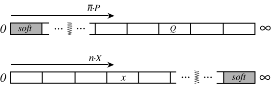
FIG. 1.: Typical momenta/positions for soft particles (shaded bins), and collinear particles (white bins).

The situation becomes interesting when we consider what form gauge invariance takes in this effective theory. Consider a bilinear quark operator $\bar{\psi}_{c}\psi_{s}$, where $\psi_{s}$ is soft and $\psi_{c}$ is collinear. If we want the collinear particle at $X\!=\!x$ and the soft particle at $X\!=\!\infty$ then gauge invariance requires them to be connected by a Wilson line $W$, so the operator is $\bar{\psi}_{c}(x)W(x,\infty)\psi_{s}(\infty)$. In QCD a gauge transformation takes $W(x,y)\to e^{i\alpha(x)}W(x,y)e^{-i\alpha(y)}$. Now, consider a “collinear” gauge transformation which has no support at $\infty$, so that $e^{-i\alpha(\infty)}\!=\!1$. The change of collinear quarks under this transformation is what requires the presence of collinear gluons. A collinear gluon cannot interact with soft particles without taking them far offshell, so $\psi_{s}(\infty)$ does not transform. The transformation simply connects $\bar{\psi}_{c}(x)$ to $W(x,\infty)$. In momentum space, the collinear gluon fields in $W$ and the collinear quark field $\psi_{c}$ are labelled by their large momenta, corresponding to the bins in Fig. 1. From matching, the bilinear quark operator can be multiplied by a complicated short distance function of these momenta $C(\bar{n}\cdot p_{i})$. However, the collinear gauge symmetry greatly restricts this function, and gives the effective theory framework predictive power.

In section II we set up a formalism which makes it simple to construct invariant field operators. This is done with the help of an operator $\bar{\cal P}$ which acts in the label space of collinear fields. This insight allows a simple set of rules to be derived, from which the most general allowed operators involving collinear fields can be constructed. This includes both leading as well as power suppressed contributions. For simplicity we focus on collinear gluons, although including soft gluons does not alter any of the results presented.

In section III we give two simple examples of how the formalism is useful. We construct a compact gauge invariant expression for the collinear quark kinetic term, and discuss the lowest order heavy-to-light weak currents in the effective theory.

In section IV we discuss a non-trivial example by constructing effective theory operators for the decays $B^{0}\to D^{+}\pi^{0}$ and $B^{-}\to D^{0}\pi^{-}$. The authors of Ref. [4, 5] proposed that at leading order in $1/E_{\pi}$ and $1/m_{b,c}$, the terms that break naive factorization for these decays are computable perturbatively. They put forth a generalized notion of factorization, in which the matrix element of a four-quark operator can be written as the product of a $B\to D$ form factor, and the convolution of a short distance coefficient with the light cone wave function of the pion. In Ref. [6] it was shown that at two-loops the only non-zero long distance contributions which could spoil generalized factorization come from the hard-soft and hard-collinear regions of phase space. However, it was shown [6] that the former give a one-loop hard coefficient times the one-loop correction to the $B\to D$ form factor, while the latter reduce to a convolution of the one-loop short distance coefficient and the one-loop pion wavefunction [7]. Here we show that the allowed operators in the effective theory reproduce the hard-collinear contribution in a simple way, and also extend the resulting convolution to include the short distance coefficient at an arbitrary order in perturbation theory.

II Invariant Operators

To explore the nature of collinear interactions we begin by taking a free field $\phi(x)$ with the mode expansion written with a relativistic measure

$$\phi(x) = \int\frac{d^{4}P}{(2\pi)^{3}}\>\delta(P\,^{2})\,\theta(P^{0})\,\bigg{[}{\cal X}(P)\>a\mbox{$(P)$}\,e^{-iP\cdot x}+{\cal Y}(P)\>b^{\dagger}\mbox{$(P)$}\,e^{iP\cdot x}\bigg{]}\equiv\phi^{+}(x)+\phi^{-}(x)\,.$$ (1)

Here $a\mbox{$(P)$}$ annihilates particles, $b^{\dagger}\mbox{$(P)$}$ creates antiparticles, and ${\cal X}(P)$ and ${\cal Y}(P)$ take values depending on the representation of the Lorentz group to which $\phi$ belongs (spinors, polarization vectors, etc.). When $P$ is collinear it scales as $P=(P^{+},P^{-},P^{\perp})\sim Q(\lambda^{2},1,\lambda)$ where $Q$ is a large scale and $\lambda$ is small. To define the effective theory the order $\lambda^{0}$ momenta must be singled out, since it is these momenta we wish to expand about. Therefore we let $P=p+k$ where $p$ includes the $\lambda^{0}$ part of $P^{-}$ and the $\lambda$ part of $P^{\perp}$, leaving $k^{\mu}\sim\lambda^{2}$. We include the $P^{\perp}$ momenta in $p$ mostly as a matter of convenience; making these momenta explicit simplifies the power counting [2]. The large phases in Eq.(1) can now be removed by defining effective theory fields $\phi^{\pm}_{n,p}$ with labels $n$ and $p$ (where $n$ defines the light cone vector the particle is moving along). Thus,

$$\phi^{+}(x) \to \sum_{p}e^{-ip\cdot x}\phi^{+}_{n,p}(x)\,,\qquad\quad\phi^{-}(x)\to\sum_{p}e^{ip\cdot x}\phi^{-}_{n,p}(x)\,,$$ (2)

$$\phi^{+}_{n,p}(x) = \int\frac{d^{4}k}{(2\pi)^{3}}\,\theta(\bar{n}\!\cdot\!p)\>\delta(n\!\cdot\!k\,\bar{n}\!\cdot\!p+p_{\perp}^{2})\>\tilde{\cal X}_{p}(k)\>a_{p}(k)\>e^{-ik\cdot x}\,,$$ (3)

$$\phi^{-}_{n,p}(x) = \int\frac{d^{4}k}{(2\pi)^{3}}\,\theta(\bar{n}\!\cdot\!p)\>\delta(n\!\cdot\!k\,\bar{n}\!\cdot\!p+p_{\perp}^{2})\>\tilde{\cal Y}_{p}(k)\>b^{\dagger}_{p}(k)\>e^{ik\cdot x}\,.$$ (4)

Since $n\cdot p=0$, only particles with large momentum $p$ in the $n^{\mu}$ direction are described. The field $\phi^{+}_{n,p}$ destroys such particles and $\phi^{-}_{n,p}$ creates the corresponding anti-particles. All fields are created or destroyed with residual momentum $k$. To simplify the notation we define

$$\phi_{n,p}(x)\equiv\phi^{+}_{n,p}+\phi^{-}_{n,-p}\,,$$ (5)

so that $\phi_{n,p}$ with positive (negative) label $\bar{n}\!\cdot\!p$ denotes the particle (antiparticle) field. The ${\cal O}(\lambda^{0})$ momentum labels on fields correspond to the bins in Fig. 1.

In Eq. (2) we have expanded about the large light cone momentum which is the meaning of the tilde in the effective theory functions $\tilde{\cal X}_{p}$ and $\tilde{\cal Y}_{p}$. For collinear fermions, the field $\xi_{n,p}$ satisfies $n\!\!\!/\xi_{n,p}=0$, and therefore has only two components. For collinear gluons the effective theory fields satisfy $(A^{\mu}_{n,q})^{*}=A^{\mu}_{n,-q}$.

If the labels $p$ were conserved quantum numbers in this large energy limit of QCD, the remainder of the discussion would be simple. The situation would be much like the velocity label $v$ on the effective theory fields in heavy quark effective theory (HQET) [8]. However, in our case the interaction of infrared degrees of freedom still cause order one changes in the labels due to the peculiar nature of light cone coordinates; since $P\,^{2}\simeq p^{-}k^{+}$, even a small change in $P\,^{2}$ can change the large $\lambda^{0}$ momentum $p^{-}$ by an amount of order one. For this reason it might seem that the decomposition in Eq. (2) is not very useful. For instance, in loop integrals we will still need to perform the sum over the large $p^{-}$ momenta.

The key observation is that after expanding, the remnant of gauge symmetry provides important restrictions on the allowed form of label changing operators. It is these restrictions that make the effective theory predictive, and determining the corresponding rules is the goal of this paper.

To proceed, we make a brief diversion to define an operator $\bar{\cal P}$ which acts on products of effective theory fields. When acting on collinear fields, $\bar{\cal P}$ gives the sum of large labels on fields minus the sum of large labels on conjugate fields. Thus, for any function $f$

$$f(\bar{\cal P})\Big{(}\phi^{\dagger}_{q_{1}}\cdots\phi^{\dagger}_{q_{m}}\phi_{p_{1}}\cdots\phi_{p_{n}}\Big{)}$$ (6)

$$\qquad=f(\bar{n}\!\cdot\!p_{1}\!+\!\ldots\!+\!\bar{n}\!\cdot\!p_{n}\!-\!\bar{n}\!\cdot\!q_{1}\!-\!\ldots\!-\!\bar{n}\!\cdot\!q_{m})\Big{(}\phi^{\dagger}_{q_{1}}\cdots\phi^{\dagger}_{q_{m}}\phi_{p_{1}}\cdots\phi_{p_{n}}\Big{)}\,.$$ (7)

The operator $\bar{\cal P}$ has mass dimension $1$, but power counting dimension $\lambda^{0}$. The conjugate operator $\bar{\cal P}^{\dagger}$ acts only to its left and gives the sum of labels on conjugate fields minus the sum of labels on fields. For convenience we also define an operator ${\cal P}_{\perp}^{\mu}\sim\lambda$ which produces the analogous sum of order $\lambda$ labels, and we let ${\cal P}^{\mu}=\frac{1}{2}n^{\mu}\bar{\cal P}+{\cal P}_{\perp}^{\mu}$.

The power counting for collinear quark fields is $\xi_{n,p}\sim\lambda$, while for collinear gluon fields $(A^{+}_{n,q},A^{-}_{n,q},A^{\perp}_{n,q})\sim(\lambda^{2},1,\lambda)$ [2]. Since $\bar{n}\!\cdot\!A_{n,q}\sim\lambda^{0}$ an operator at a given order can contain any number of these gluons. The utility of ${\cal P}^{\mu}$ is that even in an operator with an arbitrary number of fields the large phases can all be pulled to the front of the operator. This is because these phases can be commuted through derivatives,

$$i\partial^{\mu}\>e^{-ip\cdot x}\phi_{n,p}(x)=e^{-ip\cdot x}({\cal P^{\mu}}+i\partial^{\mu})\phi_{n,p}(x)\,,$$ (8)

and the overall phase then simply enforces label conservation. The remaining derivatives on fields are order $\lambda^{2}$. Furthermore, using these operators we no longer need to write explicit sums over labels. Since $\bar{\cal P}^{\mu}$ commutes with the sums, we can adopt a convention where all field labels are summed over, $\sum_{p}\phi_{n,p}\to\phi_{n,p}$. For e.g., $\sum_{p}\bar{\cal P}\phi_{n,p}=\bar{\cal P}\sum_{p}\phi_{n,p}\to\bar{\cal P}\phi_{n,p}$. From now on labels are always summed over, unless otherwise stated. This leads to our first two rules which are in some manner notational:

1. Changes of variable on the labels of fields are allowed. (The original summation variable was after all arbitrary.)
   

2. In writing Feynman rules the label momenta must be conserved.

An example of using 1) is: $\bar{n}\!\cdot\!t\>\phi_{n,r}\,\phi_{n,s-r}\,\phi_{n,t}=\bar{n}\!\cdot\!u\>\phi_{n,r}\,\phi_{n,s-r}\,\phi_{n,u}=\bar{n}\!\cdot\!u\>\phi_{n,r}\,\phi_{n,s}\,\phi_{n,u}$. Taking matrix elements and using rule 2) each term gives the same Feynman rule.

Now consider a non-abelian gauge transformation $U(x)=\exp[{i\alpha^{A}(x)T^{A}}]$ with all of its support over a set of collinear momenta. Much like in Eq. (2) it is useful to decompose this collinear transformation into a sum over these collinear momenta

$$U(x)=\sum_{Q}e^{-iQ\cdot x}{\cal U}_{Q}\,.$$ (9)

Expanding the QCD gauge transformation and using rules 1) and 2) yields particularly simple transformation rules for collinear fermions and gluons (for fixed labels $p$ and $q$)

$$\xi_{n,p} \to {\cal U}_{p-Q}\ \xi_{n,Q}\,,\qquad A^{\mu}_{n,q}\to{\cal U}_{Q}\>A^{\mu}_{n,R}\>{\cal U}^{\dagger}_{Q+R-q}+\frac{1}{g}\,{\cal U}_{Q}\Big{[}{\cal P}^{\mu}\>{\cal U}^{\dagger}_{Q-q}\Big{]}\,.$$ (10)

The square bracket indicates that ${\cal P}^{\mu}$ acts only on terms within the bracket. In general ${\cal P}^{\mu}{\cal O}=[{\cal P}^{\mu}{\cal O}]+{\cal O}{\cal P}^{\mu}$. For an Abelian gauge group Eq. (10) agrees with Ref. [2].

It is convenient to define a function $W$ of $\bar{n}\!\cdot\!A_{n,q}$ such that $W^{\dagger}\>\xi_{n,p}$ is invariant under the transformation in Eq. (10). Consider

$$W = \bigg{[}\lower 7.0pt\hbox{ $\stackrel{{\scriptstyle\sum}}{{\mbox{perms}}}$ }\!\!\exp\bigg{(}-\!g\,\frac{1}{\bar{\cal P}}\ \bar{n}\!\cdot\!A_{n,q}\bigg{)}\bigg{]}\,,\qquad\quad W^{\dagger}=\bigg{[}\lower 7.0pt\hbox{ $\stackrel{{\scriptstyle\sum}}{{\mbox{perms}}}$ }\!\!\exp\bigg{(}-\!g\,\bar{n}\!\cdot\!A^{*}_{n,q}\ \frac{1}{\bar{\cal P}^{\dagger}}\ \bigg{)}\bigg{]}\,,$$ (11)

which satisfy $W^{\dagger}W=1$. In the expansion of the exponential the $1/\bar{\cal P}$ acts to the right on all gluon fields in the square brackets, and we sum over permutations of the gluon fields. In Feynman rules the $1/n!$ in this expansion cancels the $n!$ from the choices for contracting the gluons. It is easy to show that $W$ satisfies the linear equation

$$\bigg{[}\Big{(}\bar{\cal P}+g\bar{n}\!\cdot\!A_{n,q}\Big{)}W\bigg{]}=0\,.$$ (12)

With a given boundary condition the solution of this equation is unique. Now consider

$$\bigg{[}\bigg{(}\bar{\cal P}\>+g\bigg{\{}{\cal U}_{Q}\>\bar{n}\!\cdot\!A_{n,R}\>{\cal U}^{\dagger}_{Q+R-q}+\frac{1}{g}{\cal U}_{Q}\Big{[}{\bar{\cal P}}\,{\cal U}^{\dagger}_{Q-q}\Big{]}\bigg{\}}\bigg{)}{\cal U}_{T}W\bigg{]}$$ (13)

$$=\bigg{[}\bigg{(}{\cal U}_{T}\,\{\bar{n}\!\cdot\!T+\bar{\cal P}\}+g{\cal U}_{Q}\,\bar{n}\!\cdot\!A_{n,R}\,{\cal U}^{\dagger}_{-q}\,{\cal U}_{T}+\bar{n}\!\cdot\!(q-Q)\>{\cal U}_{Q}\,{\cal U}^{\dagger}_{Q-q}\,{\cal U}_{T}\bigg{)}W\bigg{]}$$ (14)

$$=\bigg{[}\bigg{(}{\cal U}_{T}\,\{\bar{n}\!\cdot\!T+\bar{\cal P}\}+g{\cal U}_{Q}\,\bar{n}\!\cdot\!A_{n,R}-\bar{n}\!\cdot\!Q\>{\cal U}_{Q}\,{\cal U}^{\dagger}_{-q}\,{\cal U}_{T}\bigg{)}W\bigg{]}$$ (15)

$$=\bigg{[}{\cal U}_{T}(\bar{\cal P}+g\bar{n}\!\cdot\!A_{n,R})W\bigg{]}=0\,.$$ (16)

In the second line we have used (for fixed $p$) $\bar{\cal P}\phi_{n,p}=[\bar{\cal P}\phi_{n,p}]+\phi_{n,p}\bar{\cal P}=\phi_{n,p}(\bar{n}\!\cdot\!p+\bar{\cal P})$. To obtain the third and fourth lines unitarity of the gauge transformation ${\cal U}^{\dagger}_{P+r}\ {\cal U}^{\phantom{*}}_{P+r^{\prime}}=\delta_{r,r^{\prime}}$ (with fixed $r$, $r^{\prime}$) was used. We see that ${\cal U}_{T}W$ is a solution of the linear equation with $(\bar{\cal P}+g\bar{n}\,\!\cdot\!A_{n,q})$ transformed using Eq. (10). Thus, from uniqueness the transformation is

$$W\to{\cal U}_{T}W\,,$$ (17)

which makes $W^{\dagger}\xi_{n,p}$ invariant under a collinear gauge transformation. Actually, $\bar{\xi}_{n,p}W\delta_{\bar{\cal P}^{\dagger},P}$ is the Fourier transform of the quantity $\bar{\xi}_{n}(x)W(x,\infty)$ discussed in section I ($\delta$ is a Kronecker of delta). Eq. (12) is the parallel transport equation for the momentum space Wilson line $W$. Invariant operators with other fields can also be constructed, for instance the order $\lambda$ quantity $({\cal{P\!\!\!\!\hskip 1.13791pt/}}_{\perp}+gA\!\!\!/_{n,q}^{\perp})$ acts like a covariant derivative. We have (for fixed $p$)

$${\cal{P\!\!\!\!\hskip 1.13791pt/}}_{\perp}\,\xi_{n,p}+gA\!\!\!/_{n,Q}^{\perp}\,\xi_{n,p-Q}\ \to\ {\cal U}_{p-T}({\cal{P\!\!\!\!\hskip 1.13791pt/}}_{\perp}\,\xi_{n,T}+gA\!\!\!/_{n,Q}^{\perp}\,\xi_{n,T-Q})\,.$$ (18)

Wilson coefficients in an effective theory depend on the large scales, and therefore in our case on the $\bar{n}\!\cdot\!p$ labels on the fields. Since the collinear theory does not conserve labels, the Wilson coefficients can depend on $\bar{\cal P}$ and $\bar{\cal P}^{\dagger}$ and have to be inserted between the fields in an operator. In fact, invariance under Eq. (10) ensures that only the linear combination of labels picked out by $\bar{\cal P}$ and $\bar{\cal P}^{\dagger}$ can appear in these coefficients. For a function $f$, Eq. (12) can be used to prove that

$$f(\bar{\cal P}+g\bar{n}\!\cdot\!A_{n,q})=W\ f(\bar{\cal P})\ W^{\dagger}\,,$$ (19)

which guarantees that gauge invariant combinations of $\bar{n}\!\cdot\!A_{n,q}$ fields only appear in $W$. We conclude that the most general allowed operators must satisfy two more rules:

1. Only operators invariant under the transformations in Eq. (10) are allowed.
   

2. Wilson coefficients are functions of the label operators $\bar{\cal P}$ and $\bar{\cal P}^{\dagger}$ and must be inserted in all possible locations in a field operator that are consistent with 3).

III Simple examples

Our first example of the constraints imposed by the collinear gauge transformation is the kinetic term for collinear quarks. In Ref. [2] an action was constructed which gave the free propagator $i(n\!\!\!//2)/[n\cdot k+p_{\perp}^{2}/(\bar{n}\cdot p)]$ for collinear quarks, as well as their leading interactions with collinear gluons. However, because of the infinite number of couplings to $\bar{n}\!\cdot\!A_{n,q}$ gluons a closed form expression for the ${\cal O}(\lambda^{0})$ Lagrangian was not found. Such a closed gauge invariant form is easily deduced in terms of the label operators

$${\cal L} = \Bigg{[}\bar{\xi}_{n,p^{\prime}}\>\bigg{\{}n\!\cdot i{\partial}+gn\!\cdot\!A_{n,q}\,+\Big{(}{\cal{P\!\!\!\!\hskip 1.13791pt/}}_{\perp}+gA\!\!\!/_{n,q}^{\perp}\Big{)}\,W\ \frac{1}{\bar{\cal P}}\ W^{\dagger}\,\Big{(}{\cal{P\!\!\!\!\hskip 1.13791pt/}}_{\perp}+gA\!\!\!/_{n,q^{\prime}}^{\perp}\Big{)}\bigg{\}}\frac{\bar{n}\!\!\!/}{2}\,\xi_{n,p}\Bigg{]}\,,$$ (20)

where the fields are all functions of $x$. To make the dimensions consistent two powers of $\Big{(}{\cal{P\!\!\!\!\hskip 1.13791pt/}}_{\perp}+gA\!\!\!/_{n,q}^{\perp}\Big{)}$ must be accompanied by a $1/\bar{\cal P}$. The $1/\bar{\cal P}$ sits between the fields; it can not appear in front since the sum of $\bar{n}\cdot p$ momenta is zero by label conservation. Now, the gauge transformation on collinear fermions induces factors that do not commute with functions of $\bar{\cal P}$, requiring the presence of the $W^{\dagger}$ and $W$ to give an invariant operator. Thus, the factors to the left and right of the $1/\bar{\cal P}$ are separately invariant. The order $\lambda^{0}$ interactions with collinear quarks include all components of $A_{n,q}^{\mu}$ and reproduce those in Ref. [2]. Expanding the $W^{\prime}s$ in $g$ gives an infinite set of couplings to $\bar{n}\cdot A_{n,q}$ gluons.

Next, consider the example of currents with one heavy and one collinear quark field. These currents are relevant for $B$ decays to highly energetic light hadrons such as $B\to K^{*}\ell^{+}\ell^{-}$ and $B\to\pi\ell\nu$. For example, they give the soft form factor for heavy to light decays, in which only soft gluons with momenta $\sim\!\!\Lambda_{\rm QCD}$ interact with the spectator in the $B$. The exchange of a hard gluon with the spectator can induce operators with more than one collinear quark field, but these will not be considered here. The heavy-to-light current at leading order in the effective theory is

$$J^{\Gamma}=\bigg{[}\bar{\xi}_{n,p}\>W\>\Gamma\>h_{v}\ C^{\Gamma}\!(\mu,\bar{\cal P}^{\dagger})\bigg{]}\,,$$ (21)

where $h_{v}$ is the heavy quark HQET field, $\Gamma$ is one of the four independent spin structures[10, 2], and the Wilson coefficient $C^{\Gamma}$ depends on $m_{b}$, $\mu$, and $\bar{\cal P}^{\dagger}$. Invariance under collinear gauge transformations forces the combination $\bar{\xi}_{n,p}W$ to be kept together, and $C^{\Gamma}$ only appears as an overall factor. Since $\bar{\cal P}^{\dagger}$ does not act on $h_{v}$ it picks out the sum of large momenta from the collinear quark and gluons, so Eq. (21) reproduces the result in Ref. [2]. Since $C^{\Gamma}$ is only a function of the total large momentum it will never depend on a collinear loop momentum and always factors outside of loops with collinear gluons.

The effective theory pion state $|\pi_{n,p_{\pi}}\rangle$ is labelled by its large light cone momentum $p_{\pi}^{\mu}=E_{\pi}n^{\mu}$. For a function $f$, the operator $\bar{\cal P}$ acts on this state so that (for fixed $p_{\pi}$)

$$f(\bar{\cal P})\Big{|}\pi_{n,p_{\pi}}\Big{\rangle}=f(\bar{n}\cdot p_{\pi})\Big{|}\pi_{n,p_{\pi}}\Big{\rangle}=f(2E_{\pi})\Big{|}\pi_{n,p_{\pi}}\Big{\rangle}\,.$$ (22)

Therefore, in the effective theory the matrix element of the current

$$\Big{\langle}\pi_{n,p_{\pi}}\Big{|}\Big{[}\bar{\xi}_{n,p}\>W\>\Gamma\>h_{v}\ C^{\Gamma}\!(\mu,\bar{\cal P}^{\dagger})\Big{]}\Big{|}H_{v}\Big{\rangle}$$ (23)

$$\qquad=\bigg{[}\Big{\langle}\pi_{n,p_{\pi}}\Big{|}C^{\Gamma}\!(\mu,\bar{\cal P}^{\dagger})\bigg{]}\bar{\xi}_{n,p}\>W\>\Gamma\>h_{v}\ \Big{|}H_{v}\Big{\rangle}-\Big{\langle}\pi_{n,p_{\pi}}\Big{|}\bar{\xi}_{n,p}\>W\>\Gamma\>h_{v}\ \bigg{[}C^{\Gamma}\!(\mu,\bar{\cal P})\Big{|}H_{v}\Big{\rangle}\bigg{]}$$ (24)

$$\qquad=C^{\Gamma}\!(\mu,2E_{\pi})\>\Big{\langle}\pi_{n,p_{\pi}}\Big{|}\bar{\xi}_{n,p}\>W\>\Gamma\>h_{v}\Big{|}H_{v}\Big{\rangle}\,,$$ (25)

where we used momentum conservation, $\langle\pi_{n,p_{\pi}}|J^{\Gamma}\,|H_{v}\rangle\,\bar{\cal P}^{\dagger}=0$, and the fact that the heavy meson state has no large label. This explains how the Wilson coefficient ends up depending on the scale $E_{\pi}$, even though this is not the energy of any individual parton in the current.

IV The decays $\bar{B}^{0}\to D^{+}\pi^{-}$ and $B^{-}\to D^{0}\pi^{-}$

The kinematics of $B\to D\pi$ dictate that the energy of the pion is large compared to its mass. The quarks in the pion can therefore be described by collinear fermions in the effective theory. In the full theory the relevant weak Hamiltonian at $\mu_{0}=m_{b}$ is given in terms of four-quark operators ${\cal O}_{\bf 0,8}(m_{b})$

$$H_{W} = {4G_{F}\over\sqrt{2}}V_{cb}^{\phantom{*}}\,V_{ud}^{*}\bigg{[}C^{\rm full}_{\bf 0}\left(m_{b}\right)O_{\bf 0}(m_{b})+C^{\rm full}_{\bf 8}\left(m_{b}\right)O_{\bf 8}(m_{b})\bigg{]},$$ (26)

$$O_{\bf 0}(m_{b}) = ({\bar{c}\,\gamma^{\mu}P_{L}\,b})({\bar{d}\,\gamma_{\mu}P_{L}\,u}),\qquad O_{\bf 8}(m_{b})=({\bar{c}\,\gamma^{\mu}P_{L}T^{A}\,b})({\bar{d}\,\gamma_{\mu}P_{L}T^{A}\,u})\,,$$ (27)

where $P_{L}=(1-\gamma_{5})/2$. We wish to match $O_{\bf 0,8}(m_{b})$ onto operators in the effective theory. At leading order, the most general operators which satisfy the rules in section II are

$$Q_{\bf 0}^{\{1,5\}} = \Big{(}\bar{h}_{v^{\prime}}^{(c)}\>\frac{n\!\!\!/}{2}\{1,\gamma_{5}\}\>h^{(b)}_{v}\Big{)}\Big{(}\bar{\xi}_{n,p^{\prime}}^{(d)}\>W\,C_{\bf 0}^{\{1,5\}}(\mu,v\!\cdot\!v^{\prime},\bar{\cal P},\bar{\cal P}^{\dagger})\,\frac{\bar{n}\!\!\!/}{2}P_{L}\,W^{\dagger}\xi^{(u)}_{n,p}\Big{)}\,,$$ (28)

$$Q_{\bf 8}^{\{1,5\}} = \Big{(}\bar{h}_{v^{\prime}}^{(c)}\>\frac{n\!\!\!/}{2}\{1,\gamma_{5}\}\,T^{A}\>h^{(b)}_{v}\Big{)}\Big{(}\bar{\xi}_{n,p^{\prime}}^{(d)}\>W\,C_{\bf 8}^{\{1,5\}}(\mu,v\!\cdot\!v^{\prime},\bar{\cal P},\bar{\cal P}^{\dagger})\,\frac{\bar{n}\!\!\!/}{2}P_{L}\,T^{A}\,W^{\dagger}\xi^{(u)}_{n,p}\Big{)}\,.$$ (29)

The combinations $\bar{\xi}_{n,p^{\prime}}W$ and $W^{\dagger}\xi_{n,p}$ are separately invariant under Eq. (10), so the most general operator involves a Wilson coefficient inserted between these two terms. (An overall $C(\bar{\cal P})$ can be absorbed into a $C(\bar{\cal P},\bar{\cal P}^{\dagger})$ on the inside.) In general, $C_{\bf 0,8}$ depend on $\mu$, $m_{b}$, $m_{c}$, $v\!\cdot\!v^{\prime}$, and the operators $\bar{\cal P}_{\pm}=\bar{\cal P}^{\dagger}\pm\bar{\cal P}$.

In Ref. [6] it was shown that at two-loops all long distance contributions to $B\to D\pi$ can be absorbed into the $B\to D$ form factor and the light-cone pion wavefunction. Graphs with only collinear and soft ($k^{\mu}\ll Q$) gluons which could break factorization were shown to sum up to zero. Mixed hard-soft graphs reduce to the one-loop hard coefficient times the one-loop correction to the $B\to D$ form factor. Finally, mixed hard-collinear two-loop graphs also contribute, but it was shown that the result can be written as the convolution of the one-loop short distance coefficient with the one-loop Brodsky-Lepage light-cone pion wavefunction [7]. In the remainder of this section we show that the allowed form of $Q_{\bf 0}^{1}$ reproduces this convolution from one-loop graphs in the effective theory.

By parity $Q_{\bf 0}^{5}$ does not contribute, and we leave the discussion of $Q_{\bf 8}^{i}$ to Ref. [11]. In the matrix element for $B\to D\pi$ momentum conservation implies we can set $\bar{\cal P}^{\dagger}\!-\!\bar{\cal P}\!=2E_{\pi}$, similar to the example in section III. Furthermore, with $m_{\pi}=0$ the kinematics of $B\to D\pi$ can be used to eliminate $v\!\cdot\!v^{\prime}$ and $E_{\pi}$ in favor of $m_{c}$ and $m_{b}$. Therefore, we write $C^{1}_{\bf 0}(\mu,v\!\cdot\!v^{\prime},{\bar{\cal P}},{\bar{\cal P}^{\dagger}})\equiv C_{\bf 0}(\mu,{\bar{\cal P}_{+}})$. The example in this section is nontrivial because $C_{\bf 0}$ still depends on $\bar{\cal P}_{+}$.

The factors of $W$ contain an infinite set of terms with an arbitrary number of collinear gluons emerging from the four-fermion operator. The zero gluon Feynman rule is

$$= \quad i\,C_{\bf 0}\Big{(}\mu,\bar{n}\!\cdot\!(p+p^{\prime})\Big{)}\ \Gamma_{h}\otimes\Gamma_{\ell}\,.$$ (30)

where $\Gamma_{h}$ and $\Gamma_{\ell}$ are the spin structures between the heavy and light fields in $Q_{\bf 0}^{1}$. At tree level, the matching onto Eq. (30) is trivial, and $C_{\bf 0}^{(0)}(\mu,{\bar{\cal P}_{+}})=C_{\bf 0}^{\rm full}$. At one loop, matching at $\mu=m_{b}$ we find

$$C_{\bf 0}^{(1)}\Big{(}m_{b},{\bar{\cal P}_{+}}\Big{)} = C_{\bf 8}^{\rm full}\frac{C_{F}\alpha_{s}}{2\pi N_{c}}\bigg{\{}\left(3+2\ln\frac{u}{\bar{u}}\right)\ln z^{2}+f(u,z)+f(\bar{u},1/z)-b\bigg{\}}+G(z)\,,$$ (32)

in agreement with Refs. [4, 6] (where $C_{F}=4/3$ and $N_{c}=3$). Here $z={m_{c}}/{m_{b}}$, $b$ is a scheme dependent constant, the function $f(u,z)$ is given in Eq. (85) of Ref. [6], and $G(z)$ contains the standard hard contribution for the $B\to D$ form factor in HQET [12]. In our formalism $u$ and $\bar{u}$ are operators, $u=\frac{1}{2}[1+{\bar{\cal P}_{+}}/(2E_{\pi})]$ and $\bar{u}=\frac{1}{2}[1-{\bar{\cal P}_{+}}/(2E_{\pi})]$.

The new information gained from the effective theory is that the Wilson coefficients for terms with any number of collinear gluons are related to one another. They are determined by expanding the exponential $W$ factors in the operator $Q_{\bf 0}^{1}$ in Eq. (28). For example, for one gluon the Feynman rule is

$$= {ig\>\bar{n}^{\mu}}\>\Gamma_{h}\otimes\Gamma_{\ell}\>T^{A}\Bigg{\{}\frac{C_{\bf 0}\Big{(}\mu,\bar{n}\!\cdot\!(p\!+\!p^{\prime}\!+\!q)\Big{)}-C_{\bf 0}\Big{(}\mu,\bar{n}\!\cdot\!(p\!+\!p^{\prime}\!-\!q)\Big{)}}{\bar{n}\!\cdot\!q}\Bigg{\}}\,,$$ (33)

with the same function $C_{\bf 0}$ as in Eq. (30). Note that with tree level matching ($C_{\bf 0}=$ constant) the Feynman rules with $\geq 1$ gluon vanish since $W^{\dagger}W=1$.

Given the Feynman rules from Eqs. (20), (30), and (33), we can obtain the one loop contribution to $B\to D\pi$ from collinear gluon loops. The possible graphs are shown in Fig. 2. Replacing $h_{v}^{(b)}$, $h_{v^{\prime}}^{(c)}$, and $\xi_{n,p^{\prime}}^{(u)}\,\bar{\xi}_{n,p}^{(d)}$ with color singlet interpolating fields with the correct spin structure, the spin and color traces can be performed to give

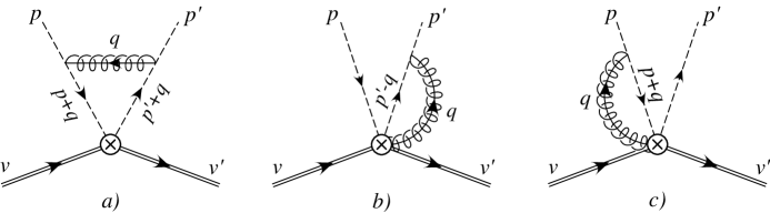
FIG. 2.: The collinear graphs contributing at one loop in the effective theory.

$$iA_{a} = 2g^{2}C_{F}\int\!\frac{d^{d}q}{(2\pi)^{d}}\>\frac{q_{\perp}^{2}}{(q+p)^{2}(q+p^{\prime})^{2}q^{2}}\ C_{\bf 0}\Big{(}\mu,\bar{n}\!\cdot\!(p+p^{\prime}+2q)\Big{)}\quad\mbox{+\, \{$p_{\perp}$, $p^{\prime}_{\perp}$\} terms}\,,$$ (35)

$$iA_{b} = -2g^{2}C_{F}\int\!\frac{d^{d}q}{(2\pi)^{d}}\>\frac{\bar{n}\!\cdot\!(p^{\prime}-q)}{q^{2}(p^{\prime}-q)^{2}}\ \frac{C_{\bf 0}\Big{(}\mu,\bar{n}\!\cdot\!(p+p^{\prime})\Big{)}-C_{\bf 0}\Big{(}\mu,\bar{n}\!\cdot\!(p+p^{\prime}-2q)\Big{)}}{\bar{n}\!\cdot\!q}\,,$$ (36)

$$iA_{c} = -2g^{2}C_{F}\int\!\frac{d^{d}q}{(2\pi)^{d}}\>\frac{\bar{n}\!\cdot\!(p+q)}{q^{2}(p+q)^{2}}\ \frac{C_{\bf 0}\Big{(}\mu,\bar{n}\!\cdot\!(p+p^{\prime}+2q)\Big{)}-C_{\bf 0}\Big{(}\mu,\bar{n}\!\cdot\!(p+p^{\prime})\Big{)}}{\bar{n}\!\cdot\!q}\,,$$ (37)

where a common prefactor is suppressed. Adopting the notation of Ref. [6], we let $q\to-q$ for the integration variable in $A_{b}$, and let $p=-\bar{u}p_{\pi}$, $p^{\prime}=up_{\pi}$, $p_{\pi}=E_{\pi}n^{\mu}$, $\bar{n}\!\cdot q\equiv 2\alpha E_{\pi}$, with $\bar{u}=1-u$, and drop the $p_{\perp}$ and $p_{\perp}^{\prime}$ dependence. The sum of the three graphs is then

$$iA_{abc} = g^{2}C_{F}\!\int\!\frac{d^{d}q}{(2\pi)^{d}}\Bigg{\{}\left[\frac{2(u\!+\!\alpha)}{\alpha}\frac{1}{(q+up_{\pi})^{2}q^{2}}-\frac{2(\bar{u}\!-\!\alpha)}{\alpha}\frac{1}{(q-\bar{u}p_{\pi})^{2}q^{2}}\right]\Big{[}T(u)\!-\!T(u\!+\!\alpha)\Big{]}$$ (39)

$$\qquad\qquad\qquad\quad+\frac{2q_{\perp}^{2}}{(q+up_{\pi})^{2}(q-\bar{u}p_{\pi})^{2}q^{2}}\>T(u\!+\!\alpha)\Bigg{\}}\,,$$

where

$$T(x,\mu)\equiv C_{\bf 0}(\mu,(4x-2)E_{\pi})\,.$$ (40)

Using the one loop result for the short distance coefficient, $T^{(1)}(x,\mu)$, Eq. (39) is exactly the result of the explicit two loop calculation given in Eq. (193) of Ref. [6]. Invariance under the collinear gauge transformation has enabled us to reproduce this result without having to calculate two loop graphs.

In Ref. [6] it was shown that after performing the $q_{\perp}$ and $n\!\cdot\!q$ integrals in Eq. (39) and adding the collinear wave function contribution, $A_{abc}$ factors into the convolution of $T^{(1)}(x,\mu)$ with the one-loop light cone pion wavefunction [7], $\Phi_{\pi}^{(1)}(x,\mu)$, i.e.

$$iA_{abc}\ +\ \ \begin{picture}(65.0,20.0)(1.0,1.0)\lower 8.0pt\hbox{\includegraphics[width=72.26999pt]{WF}} \end{picture}\ \ \ = \ \int_{0}^{1}dx\>T^{(1)}(x,\mu)\>\Phi_{\pi}^{(1)}(x,\mu)\,.$$ (41)

However, our result in Eq. (39) holds with $T(x)$ matched at any order in perturbation theory, so the same steps reduce Eq. (39) to the convolution of the complete short distance coefficient with $\Phi_{\pi}^{(1)}(x,\mu)$,

$$iA_{abc}\ +\ \ \begin{picture}(65.0,20.0)(1.0,1.0)\lower 8.0pt\hbox{\includegraphics[width=72.26999pt]{WF}} \end{picture}\ \ \ = \ \int_{0}^{1}dx\>T(x,\mu)\>\Phi_{\pi}^{(1)}(x,\mu)\,.$$ (42)

This provides strong additional evidence for the validity of generalized factorization [4, 5] for $B\to D\pi$. It also illustrates the utility of the effective theory description of collinear degrees of freedom. Within this framework an all orders proof of generalized factorization is presented in Ref. [11], where soft modes are included and the convolution discussed above is extended to include the complete non-perturbative pion light cone wavefunction.

V Conclusion

We have shown that gauge invariant operators in the collinear effective theory can be constructed by satisfying four simple rules:

1. Changes of variable on the labels of effective theory fields are allowed.
   

2. In writing Feynman rules the label momenta must be conserved.
   

3. Only operators invariant under collinear gauge transformations (Eq. (10)) are allowed.
   

4. Wilson coefficients are functions of the label operators $\bar{\cal P}$ and $\bar{\cal P}^{\dagger}$ and must be inserted in all possible locations in a field operator that are consistent with 3).
   

We have presented two simple examples by constructing the kinetic term for collinear quarks and the heavy to light current. We then showed how the formalism can be applied to the decay $B\to D\pi$. Only one color singlet operator can be constructed which contributes to this decay, and we reproduced a nontrivial two loop result in Ref. [6]. Furthermore, in the effective theory the one-loop graphs with a single collinear gluon give a convolution of the short distance coefficient at any order in perturbation theory with the one-loop pion wavefunction. Within this framework an all orders proof of generalized factorization for $B\to D\pi$ is presented in Ref. [11].

REFERENCES

• [1] C. W. Bauer, S. Fleming and M. Luke, Phys. Rev.  D63, 014006 (2001).
• [2] C. W. Bauer, S. Fleming, D. Pirjol and I. W. Stewart, Phys. Rev. D 63, 114020 (2001).
• [3] See for example: J. C. Collins and D. E. Soper, Nucl. Phys. B 194, 445 (1982); J. C. Collins, D. E. Soper and G. Sterman, Nucl. Phys. B 261, 104 (1985).
• [4] H. D. Politzer and M. B. Wise, Phys. Lett. B 257, 399 (1991).
• [5] M. Beneke, G. Buchalla, M. Neubert, and C. T. Sachrajda, Phys. Rev. Lett.  83, 1914 (1999).
• [6] M. Beneke, G. Buchalla, M. Neubert, and C. T. Sachrajda, Nucl. Phys.  B591, 313 (2000).
• [7] G. P. Lepage and S. J. Brodsky, Phys. Rev. D 22, 2157 (1980).
• [8] H. Georgi, Phys. Lett.  B240, 447 (1990).
• [9] M. J. Dugan and B. Grinstein, Phys. Lett.  B255, 583 (1991).
• [10] J. Charles, A. Le Yaouanc, L. Oliver, O. Pene, and J. C. Raynal, Phys. Rev.  D60, 014001 (1999).
• [11] C. W. Bauer, D. Pirjol and I. W. Stewart, hep-ph/0107002.
• [12] A. F. Falk, H. Georgi, B. Grinstein and M. B. Wise, Nucl. Phys. B 343, 1 (1990); A. F. Falk and B. Grinstein, Phys. Lett. B 249, 314 (1990); M. Neubert, Nucl. Phys. B 371, 149 (1992); see also M. Neubert, Phys. Rept.  245, 259 (1994).