LTH 516

Is the up-quark massless?
UKQCD Collaboration

A.C. Irving, C. McNeile, C. Michael, K.J. Sharkey and H. Wittig

Division of Theoretical Physics, Department of Mathematical Sciences, University of Liverpool, Liverpool L69 3BX, UK

We report on determinations of the low-energy constants $\alpha_{5}$ and $\alpha_{8}$ in the effective chiral Lagrangian at O($p^{4}$), using lattice simulations with $N_{\rm f}=2$ flavours of dynamical quarks. Precise knowledge of these constants is required to test the hypothesis whether or not the up-quark is massless. Our results are obtained by studying the quark mass dependence of suitably defined ratios of pseudoscalar meson masses and matrix elements. Although comparisons with an earlier study in the quenched approximation reveal small qualitative differences in the quark mass behaviour, numerical estimates for $\alpha_{5}$ and $\alpha_{8}$ show only a weak dependence on the number of dynamical quark flavours. Our results disfavour the possibility of a massless up-quark, provided that the quark mass dependence in the physical three-flavour case is not fundamentally different from the two-flavour case studied here.

1 Introduction

A massless up-quark represents a simple and elegant solution to the strong CP problem. Consequently, the question of whether or not $m_{\rm u}$ is indeed zero has been the subject of much debate over many years (for a review see ref. [1]). Traditionally the problem is studied in the framework of Chiral Perturbation Theory (ChPT). Although the most recent estimates point to a non-zero value for the ratio $m_{\rm u}/m_{\rm d}$ [2], the situation is complicated by the presence of a hidden symmetry in the effective chiral Lagrangian [3]. This so-called “Kaplan-Manohar ambiguity” implies that $m_{\rm u}/m_{\rm d}$ can only be constrained after supplementing ChPT with additional theoretical assumptions. Although the validity of the commonly used assumptions is plausible [4, 5], it is clear that the question whether the up-quark is massless cannot be studied from first principles in ChPT.

More recently attention has focussed on lattice simulations to tackle this problem. A reliable, direct lattice calculation of $m_{\rm u}$, however, presents considerable difficulties, even on today’s massively parallel computers. It was therefore proposed to use a more indirect approach, based on a combination of lattice QCD and ChPT [6, 7, 8]. The aim of this method is a lattice determination of the so-called “low-energy constants” in the effective chiral Lagrangian, whose precise values are required to constrain $m_{\rm u}/m_{\rm d}$ using chiral symmetry and phenomenological input. A variant of this proposal, which allows for a determination of the low-energy constants with good statistical accuracy was discussed in ref. [9] and tested in the quenched approximation.

Here we extend the study of [9] to QCD with two flavours of dynamical quarks. While this addresses the important issue of dynamical quark effects, it still does not correspond to the physical three-flavour case, and thus we are yet unable to give a final answer to the question in the title of this paper. Nevertheless, our study represents an important step in an ultimately realistic treatment of the problem, by studying the dependence of the low-energy constants on the number of flavours. If our results can be taken over to the physical case without large modifications – and there are indications that this is not unreasonable – then the possibility of a massless up-quark is strongly disfavoured.

In Section 2 we briefly review the Kaplan-Manohar ambiguity and its relevance for the value of $m_{\rm u}$. Section 3 contains details of our lattice simulations, whose results are described in Section 4. In Section 5 we discuss the implications of our findings and present an outlook to future work.

2 Low-energy constants and $m_{\rm u}=0$

In order to make this paper self-contained, we briefly review the implications of the Kaplan-Manohar ambiguity for the ratio $m_{\rm u}/m_{\rm d}$. The strategy to address the problem in lattice simulations will then become clear. A more complete discussion can be found in refs. [2, 5, 7, 9].

A determination of $m_{\rm u}/m_{\rm d}$ in ChPT which is able to distinguish between a massless and a massive up-quark requires precise knowledge of the first-order mass correction term $\Delta_{\rm M}$. At order $p^{4}$ in the chiral Lagrangian it is given by [10, 11, 12]

$$\Delta_{\rm M}=\frac{m_{\rm K}^{2}-m_{\pi}^{2}}{(4\pi F_{\pi})^{2}}\,(2\alpha_{8}-\alpha_{5})+\hbox{chiral logs},$$ (1)

where $F_{\pi}=93.3\,{\rm MeV}$ is the pion decay constant, and $\alpha_{5}$, $\alpha_{8}$ are low-energy constants, whose values have to be determined from phenomenology. Throughout this paper we adopt a convention in which the low-energy constants $\alpha_{i}$ are related to the corresponding constants $L_{i}$ of ref. [11] through $\alpha_{i}=8(4\pi)^{2}L_{i}$. Furthermore, we always quote low-energy constants in the ${\overline{{\rm MS}}}$-scheme at scale $\mu=4\pi F_{\pi}$.

The value of $\alpha_{5}$ can be extracted from the ratio of pseudoscalar decay constants, $F_{\rm K}/F_{\pi}$, and is given by

$$\alpha_{5}=0.5\pm 0.6.$$ (2)

By contrast, there is no direct phenomenological information on $\alpha_{8}$ or the combination $(2\alpha_{8}-\alpha_{5})$. Although $\alpha_{8}$ is contained in the correction to the Gell-Mann–Okubo formula, i.e.

$$\Delta_{\rm GMO}=\frac{m_{\rm K}^{2}-m_{\pi}^{2}}{(4\pi F_{\pi})^{2}}\,(\alpha_{5}-12\alpha_{7}-6\alpha_{8})+\hbox{chiral logs},$$ (3)

its determination requires prior knowledge of $\alpha_{7}$. It is at this point that the Kaplan-Manohar (KM) ambiguity becomes important. It arises from the observation that a simultaneous transformation of the quark masses

$$m_{\rm u}\to m_{\rm u}+\lambda m_{\rm d}m_{\rm s},\quad m_{\rm d}\to m_{\rm d}+\lambda m_{\rm s}m_{\rm u},\quad m_{\rm s}\to m_{\rm s}+\lambda m_{\rm u}m_{\rm d},$$ (4)

and coupling constants according to

$$\alpha_{6}\to\alpha_{6}+\lambda\frac{(4\pi F_{0})^{2}}{4B_{0}},\quad\alpha_{7}\to\alpha_{7}+\lambda\frac{(4\pi F_{0})^{2}}{4B_{0}},\quad\alpha_{8}\to\alpha_{8}-\lambda\frac{(4\pi F_{0})^{2}}{2B_{0}},$$ (5)

leaves the effective chiral Lagrangian invariant. Here, $\lambda$ is an arbitrary parameter, and $F_{0}$, $B_{0}$ are coupling constants in the lowest-order chiral Lagrangian. Thus, chiral symmetry cannot distinguish between different sets of quark masses and coupling constants, which are related through eqs. (4) and (5). Indeed the correction $\Delta_{\rm GMO}$ is invariant under the above transformations. The value of $\alpha_{7}$ can be fixed by invoking additional theoretical assumptions, such as the validity of large-$N_{c}$ arguments for $N_{c}=3$. In accordance with these assumptions, Leutwyler [2] constrained the correction term $\Delta_{\rm M}$ to be small and positive:

$$0<\Delta_{\rm M}\leq 0.13.$$ (6)

This gives $m_{\rm u}/m_{\rm d}=0.553(43)$ and hence a non-zero value for $m_{\rm u}$. The “standard” values for $\alpha_{7}$ and $\alpha_{8}$ which are compatible with eq. (6) are [10, 11, 12]

$$\alpha_{7}=-0.5\pm 0.25,\qquad\alpha_{8}=0.76\pm 0.4.$$ (7)

In view of the importance of the strong CP problem, one may regard any analysis based on theoretical assumptions beyond chiral symmetry as insufficient. In particular, since the uncertainties in the estimates for $\alpha_{7}$ and $\alpha_{8}$ are quite large, the possibility that $m_{\rm u}=0$ does not appear to be ruled out completely. A massless up-quark would require [7]

$$\alpha_{7}=0.25\pm 0.25,\qquad\alpha_{8}=-0.9\pm 0.4,$$ (8)

resulting in a large, negative first-order correction $\Delta_{\rm{M}}$. In order to decide which scenario is realised and to pin down the value of $m_{\rm u}$ one has to replace the theoretical assumptions by a solution of the underlying theory of QCD.

The KM ambiguity implies that the low-energy constants $\alpha_{7}$, $\alpha_{8}$ (and $\alpha_{6}$) can be determined from chiral symmetry and phenomenology only if the physical quark masses are known already. At this point it is important to realise that QCD is not afflicted with the KM ambiguity, and that the formalism of ChPT also holds for unphysical quark masses. Since quark masses are input parameters in lattice simulations of QCD, their relations to hadronic observables need not be known a priori. Hence, the low-energy constants can be determined by studying pseudoscalar meson masses and matrix elements for unphysical quark masses and fitting their quark mass dependence to the expressions found in ChPT. In this way it is possible to determine $\alpha_{5}$ and – more importantly – the combination $(2\alpha_{8}-\alpha_{5})$ directly in lattice simulations.

3 Lattice setup and simulation details

In ref. [9] it was shown how the low-energy constants can be extracted from lattice data for suitably defined ratios of pseudoscalar masses and matrix elements, $R_{\rm M}$ and $R_{\rm F}$. Here we repeat their definitions in order to explain the necessary notation. For more details we refer the reader to the original paper [9].

The actual determination of the low-energy constants proceeds by studying the mass dependence of $R_{\rm M}$ and $R_{\rm F}$ around some reference quark mass $m_{\rm ref}$. As pointed out before, $m_{\rm ref}$ does not have to coincide with a physical quark mass [13], as long as it is small enough for ChPT to be applicable.

In this paper we will be concerned with simulations of “partially quenched” QCD, where valence and sea quarks can have different masses. Let us therefore consider a pseudoscalar meson with valence quark masses $m_{1}$ and $m_{2}$ at a fixed value of the sea quark mass $m^{\rm sea}$. In [9] the dimensionless mass parameters

$$y=\frac{B_{0}(m_{1}+m_{2})}{(4\pi F_{0})^{2}},\quad y_{\rm ref}=\frac{2B_{0}m_{\rm ref}}{(4\pi F_{0})^{2}},\quad x=y/y_{\rm ref},$$ (9)

were defined, as well as the ratios

$$R_{\rm M}(x) = \left(\frac{F_{\rm PS}(y)}{G_{\rm PS}(y)}\right)\left/\left(\frac{F_{\rm PS}(y_{\rm ref})}{G_{\rm PS}(y_{\rm ref})}\right)\right.$$

$$R_{\rm F}(x) = F_{\rm PS}(y)\left/F_{\rm PS}(y_{\rm ref})\right.,\qquad x=y/y_{\rm ref}.$$ (10)

Here $F_{\rm PS}$ is the pseudoscalar decay constant, and $G_{\rm PS}$ is the matrix element of the pseudoscalar density between a pseudoscalar state and the vacuum. The parameter $x$ denotes the fraction of the reference quark mass at which the ratios $R_{\rm M}$ and $R_{\rm F}$ are considered.

As emphasised in [9], $R_{\rm M}$ and $R_{\rm F}$ are well-suited to extract the low-energy constants, since ratios are usually obtained with high statistical accuracy in numerical simulations. Furthermore, any renormalisation factors associated with $F_{\rm PS}$ and $G_{\rm PS}$ drop out, so that $R_{\rm M}$ and $R_{\rm F}$ can be readily extrapolated to the continuum for every fixed value of $x$. As has been shown in the quenched approximation [9], discretisation errors in $R_{\rm M}$ and $R_{\rm F}$ are very small, so that good control over lattice artefacts is achieved. This issue is important, since the determination of low-energy constants requires an unambiguous separation of the mass dependence from effects of non-zero lattice spacing.

We now give the expressions for $R_{\rm M}$ and $R_{\rm F}$ in partially quenched QCD which are relevant for our study. They were obtained using the results of ref. [14] and are listed in appendix A of [9]. Our reference point $y_{\rm ref}$ was always defined at

$$m_{1}=m_{2}=m^{\rm sea}=m_{\rm ref},\quad y_{\rm ref}=\frac{2B_{0}m_{\rm ref}}{(4\pi F_{0})^{2}}.$$ (11)

In order to map out the mass dependence of $R_{\rm M}$ and $R_{\rm F}$ for a fixed value of $m^{\rm sea}$, we have considered the cases labelled “VV” and “VS1” in ref. [9]. The first uses degenerate valence quarks and is defined by

$$\hbox{VV:}\quad m_{1}=m_{2}=xm_{\rm ref},\quad m^{\rm sea}=m_{\rm ref},$$ (12)

which leads to the expressions

$$R_{\rm M}^{\rm VV}(x) = 1-\frac{1}{N_{\rm f}}y_{\rm ref}\left[(2x-1)\ln{x}+2(x-1)\ln y_{\rm ref}\right]$$ (13)

$$-y_{\rm ref}(x-1)\left[(2\alpha_{8}-\alpha_{5})+\textstyle\frac{1}{N_{\rm f}}\right]$$

$$R_{\rm F}^{\rm VV}(x) = 1-\frac{N_{\rm f}}{4}y_{\rm ref}\left[(x+1)\ln\left(\textstyle\frac{1}{2}(x+1)\right)+(x-1)\ln y_{\rm ref}\right]$$ (14)

$$+y_{\rm ref}(x-1)\textstyle\frac{1}{2}\alpha_{5},$$

where $N_{\rm f}$ denotes the number of dynamical quark flavours. The case labelled “VS1”, based on non-degenerate valence quarks, is defined by

$$\hbox{VS1:}\quad m_{1}=xm_{\rm ref},\quad m_{2}=m^{\rm sea}=m_{\rm ref}.$$ (15)

According to Table 1 of ref. [9] the expressions for the ratios are then given by

$$R_{\rm M}^{\rm VS1}(x) = 1-\frac{1}{N_{\rm f}}y_{\rm ref}\left[x\ln{x}+(x-1)\ln y_{\rm ref}\right]-y_{\rm ref}(x-1)\textstyle\frac{1}{2}(2\alpha_{8}-\alpha_{5})$$ (16)

$$R_{\rm F}^{\rm VS1}(x) = 1-\frac{N_{\rm f}}{8}y_{\rm ref}\left[(x+1)\ln\left(\textstyle\frac{1}{2}(x+1)\right)+(x-1)\ln y_{\rm ref}+\textstyle\frac{2}{N_{\rm f}^{2}}\ln{x}\right]$$ (17)

$$+y_{\rm ref}(x-1)\textstyle\frac{1}{4}\left(\alpha_{5}+\textstyle\frac{1}{N_{\rm f}}\right).$$

Our simulations were performed for $N_{\rm f}=2$ flavours of dynamical, O($a$) improved Wilson fermions. The value of the bare coupling was set to $\beta=6/g_{0}^{2}=5.2$. The improvement coefficient $c_{\rm sw}$, which multiplies the Sheikholeslami-Wohlert term in the fermionic action, was taken from the interpolating formula of ref. [15]. Here we considered a single value of the sea quark mass, corresponding to a hopping parameter $\mbox{$\kappa^{\rm sea}$}=0.1355$. For this choice of parameters we generated 208 dynamical gauge configurations on a lattice of size $16^{3}\cdot 32$. For further details we refer to [16, 17, 18]. Here we only mention that the hadronic radius $r_{0}$ defined through the force between static sources [19] has been determined as $r_{0}/a=5.041(40)$ [18]. For $r_{0}=0.5\,{\rm fm}$ this implies that the lattice spacing in physical units is $a=0.099(1)\,{\rm fm}$.

We have computed quark propagators for valence quarks with hopping parameters $\mbox{$\kappa^{\rm val}$}=0.1340$, 0.1345, 0.1350, 0.1355 and 0.1358. In addition to local operators, we have also calculated propagators for fuzzed sinks and/or sources, using the procedure of [20]. In the pseudoscalar channel we employed both the pseudoscalar density and the temporal component of the axial current as interpolating operators. These two types were used together with the different combinations of fuzzed and local propagators to construct a $4\times 4$ matrix correlator for pseudoscalar mesons. By performing factorising fits using an ansatz that incorporates the ground state and the first excitation, we were able to extract the pseudoscalar mass $m_{\rm PS}$, as well as the matrix elements of the axial current and the pseudoscalar density, i.e.

$$\zeta_{\rm A}=\langle 0|A_{0}|{\hbox{PS}}\rangle,\qquad\zeta_{\rm P}=\langle 0|P|{\hbox{PS}}\rangle.$$ (18)

In order to be consistent with O($a$) improvement the amplitudes $\zeta_{\rm A}$ and $\zeta_{\rm P}$ must be related to the matrix elements of the improved currents and densities at non-zero quark mass. Using the definitions of [21] it is then easy to see that the (unrenormalised) pseudoscalar decay constant is given by

$$F_{\rm PS}=(1+b_{\rm A}{am_{\rm q}})\left\{\frac{\zeta_{\rm A}}{m_{\rm PS}}+c_{\rm A}\frac{\zeta_{\rm P}}{m_{\rm PS}}\sinh(am_{\rm PS})\right\},$$ (19)

whereas $G_{\rm PS}$ is given by

$$G_{\rm PS}=(1+b_{\rm P}{am_{\rm q}})\zeta_{\rm P}.$$ (20)

The improvement coefficients $b_{\rm A}$, $b_{\rm P}$ and $c_{\rm A}$ were computed in one-loop perturbation theory [22, 23] in the bare coupling, since non-perturbative estimates are not available at present. For the improvement coefficient $c_{\rm A}$ this procedure yields

$$c_{\rm A}=-0.0087.$$ (21)

For degenerate valence quarks the quark mass $m_{\rm q}$ is given by

$$am_{\rm q}=\frac{1}{2}\left(\frac{1}{\mbox{$\kappa^{\rm val}$}}-\frac{1}{\mbox{$\kappa_{\rm crit}$}}\right),$$ (22)

where we have inserted $\mbox{$\kappa_{\rm crit}$}=0.13693$ for the critical hopping parameter, as estimated in [15]. Finally we note that the current quark mass $m$ defined through the PCAC relation in the O($a$) improved theory is obtained from $\zeta_{\rm A}$, $\zeta_{\rm P}$ and $m_{\rm PS}$ via

$$am=\frac{\zeta_{\rm A}}{2\zeta_{\rm P}}\sinh(am_{\rm PS})+\frac{1}{2}c_{\rm A}\sinh^{2}(am_{\rm PS}).$$ (23)

All our statistical errors were obtained using a bootstrap procedure [24].

4 Results

Our results for pseudoscalar masses, matrix elements and current quark masses are listed in Table 1. Compared with [18] the numbers for the pseudoscalar masses reported here may differ by up to one standard deviation, as a result of using a larger matrix correlator in the fitting procedure.

Following eq. (11) we have defined the mass $m_{\rm ref}$ at the reference point for $\kappa_{1}^{\rm val}=\kappa_{2}^{\rm{val}}=\mbox{$\kappa^{\rm sea}$}=0.1355$, which corresponds to $\left.(r_{0}m_{\rm PS})^{2}\right|_{m=m_{\rm ref}}=2.092$. Using the leading-order relations $m_{\rm PS}^{2}=2{B_{0}}m$ and $F_{0}=F_{\pi}=93.3\,{\rm MeV}$ this implies

$$y_{\rm ref}=0.2370.$$ (24)

It is instructive to compare these values with those of the previous quenched study [9], where $y_{\rm ref}=0.3398$, $(r_{0}m_{\rm PS})^{2}|_{m=m_{\rm ref}}=3$, and $m_{\rm ref}\approx m_{\rm s}$. Hence, the value of $m_{\rm ref}$ employed in this paper is smaller by 30%, such that $m_{\rm ref}\approx 0.7m_{\rm s}$. A smaller value of $m_{\rm ref}$ is clearly desirable for our purpose, since the predictions of ChPT are expected to hold more firmly for smaller masses. Nevertheless, our sea quarks are still relatively heavy, as signified by the ratio $(m_{\rm PS}/m_{\rm V})|_{m=m^{\rm sea}}\approx 0.58$ [18], which is to be compared to $m_{\pi}/m_{\rho}=0.169$.

In the spirit of partially quenched QCD we have considered valence quarks that are lighter than the sea quarks. We were thus able to extend the quark mass range down to about $m_{\rm s}/2$, which is quite a bit below the smallest mass reached in [9]. This may be an indication that the inclusion of dynamical quarks alleviates the problem of exceptional configurations, which precludes attempts to work at very small quark masses in the quenched approximation. However, our attempts to push to valence quark masses below $m_{\rm s}/2$ have proved unsuccessful, due to the appearance of exceptional configurations for $m^{\rm val}/m^{\rm sea}\;\raisebox{-2.58334pt}{$\stackrel{{\scriptstyle\textstyle{<}}}{{\sim}}$}\;0.7$. More precisely, we observed large statistical fluctuations in hadron correlators computed from quark propagators at $\kappa^{\rm{val}}=0.1360$, despite the fact that the inversion algorithm converged.

$\kappa_{1}^{\rm val}$	$\kappa^{\rm val}_{2}$		$am_{\rm PS}$	$a\zeta_{\rm A}/m_{\rm PS}$	$a^{2}\zeta_{\rm P}$	$am$
0.1358	0.1358		0.2301$\;\begin{array}[]{@{}l@{}}\makebox[15.0pt][c]{$+$}\makebox[3.85002pt][r]{52}\\[-0.83997pt] \makebox[15.0pt][c]{$-$}\makebox[3.85002pt][r]{51}\end{array}$	0.0995$\;\begin{array}[]{@{}l@{}}\makebox[15.0pt][c]{$+$}\makebox[3.85002pt][r]{24}\\[-0.83997pt] \makebox[15.0pt][c]{$-$}\makebox[3.85002pt][r]{30}\end{array}$	0.1782$\;\begin{array}[]{@{}l@{}}\makebox[15.0pt][c]{$+$}\makebox[3.85002pt][r]{70}\\[-0.83997pt] \makebox[15.0pt][c]{$-$}\makebox[3.85002pt][r]{57}\end{array}$	0.0147$\;\begin{array}[]{@{}l@{}}\makebox[15.0pt][c]{$+$}\makebox[1.04996pt][r]{4}\\[-0.83997pt] \makebox[15.0pt][c]{$-$}\makebox[1.04996pt][r]{5}\end{array}$
0.1355	0.1355		0.2869$\;\begin{array}[]{@{}l@{}}\makebox[15.0pt][c]{$+$}\makebox[3.85002pt][r]{40}\\[-0.83997pt] \makebox[15.0pt][c]{$-$}\makebox[3.85002pt][r]{41}\end{array}$	0.1068$\;\begin{array}[]{@{}l@{}}\makebox[15.0pt][c]{$+$}\makebox[3.85002pt][r]{22}\\[-0.83997pt] \makebox[15.0pt][c]{$-$}\makebox[3.85002pt][r]{25}\end{array}$	0.1893$\;\begin{array}[]{@{}l@{}}\makebox[15.0pt][c]{$+$}\makebox[3.85002pt][r]{57}\\[-0.83997pt] \makebox[15.0pt][c]{$-$}\makebox[3.85002pt][r]{52}\end{array}$	0.0232$\;\begin{array}[]{@{}l@{}}\makebox[15.0pt][c]{$+$}\makebox[1.04996pt][r]{4}\\[-0.83997pt] \makebox[15.0pt][c]{$-$}\makebox[1.04996pt][r]{5}\end{array}$
0.1350	0.1350		0.3585$\;\begin{array}[]{@{}l@{}}\makebox[15.0pt][c]{$+$}\makebox[3.85002pt][r]{26}\\[-0.83997pt] \makebox[15.0pt][c]{$-$}\makebox[3.85002pt][r]{28}\end{array}$	0.1166$\;\begin{array}[]{@{}l@{}}\makebox[15.0pt][c]{$+$}\makebox[3.85002pt][r]{20}\\[-0.83997pt] \makebox[15.0pt][c]{$-$}\makebox[3.85002pt][r]{24}\end{array}$	0.1046$\;\begin{array}[]{@{}l@{}}\makebox[15.0pt][c]{$+$}\makebox[3.85002pt][r]{47}\\[-0.83997pt] \makebox[15.0pt][c]{$-$}\makebox[3.85002pt][r]{49}\end{array}$	0.0368$\;\begin{array}[]{@{}l@{}}\makebox[15.0pt][c]{$+$}\makebox[1.04996pt][r]{4}\\[-0.83997pt] \makebox[15.0pt][c]{$-$}\makebox[1.04996pt][r]{5}\end{array}$
0.1345	0.1345		0.4192$\;\begin{array}[]{@{}l@{}}\makebox[15.0pt][c]{$+$}\makebox[3.85002pt][r]{20}\\[-0.83997pt] \makebox[15.0pt][c]{$-$}\makebox[3.85002pt][r]{23}\end{array}$	0.1246$\;\begin{array}[]{@{}l@{}}\makebox[15.0pt][c]{$+$}\makebox[3.85002pt][r]{19}\\[-0.83997pt] \makebox[15.0pt][c]{$-$}\makebox[3.85002pt][r]{24}\end{array}$	0.2187$\;\begin{array}[]{@{}l@{}}\makebox[15.0pt][c]{$+$}\makebox[3.85002pt][r]{40}\\[-0.83997pt] \makebox[15.0pt][c]{$-$}\makebox[3.85002pt][r]{45}\end{array}$	0.0507$\;\begin{array}[]{@{}l@{}}\makebox[15.0pt][c]{$+$}\makebox[1.04996pt][r]{5}\\[-0.83997pt] \makebox[15.0pt][c]{$-$}\makebox[1.04996pt][r]{5}\end{array}$
0.1340	0.1340		0.4739$\;\begin{array}[]{@{}l@{}}\makebox[15.0pt][c]{$+$}\makebox[3.85002pt][r]{17}\\[-0.83997pt] \makebox[15.0pt][c]{$-$}\makebox[3.85002pt][r]{20}\end{array}$	0.1312$\;\begin{array}[]{@{}l@{}}\makebox[15.0pt][c]{$+$}\makebox[3.85002pt][r]{17}\\[-0.83997pt] \makebox[15.0pt][c]{$-$}\makebox[3.85002pt][r]{25}\end{array}$	0.2315$\;\begin{array}[]{@{}l@{}}\makebox[15.0pt][c]{$+$}\makebox[3.85002pt][r]{43}\\[-0.83997pt] \makebox[15.0pt][c]{$-$}\makebox[3.85002pt][r]{44}\end{array}$	0.0650$\;\begin{array}[]{@{}l@{}}\makebox[15.0pt][c]{$+$}\makebox[1.04996pt][r]{6}\\[-0.83997pt] \makebox[15.0pt][c]{$-$}\makebox[1.04996pt][r]{5}\end{array}$
0.1358	0.1355		0.2607$\;\begin{array}[]{@{}l@{}}\makebox[15.0pt][c]{$+$}\makebox[3.85002pt][r]{45}\\[-0.83997pt] \makebox[15.0pt][c]{$-$}\makebox[3.85002pt][r]{46}\end{array}$	0.1033$\;\begin{array}[]{@{}l@{}}\makebox[15.0pt][c]{$+$}\makebox[3.85002pt][r]{24}\\[-0.83997pt] \makebox[15.0pt][c]{$-$}\makebox[3.85002pt][r]{26}\end{array}$	0.1841$\;\begin{array}[]{@{}l@{}}\makebox[15.0pt][c]{$+$}\makebox[3.85002pt][r]{60}\\[-0.83997pt] \makebox[15.0pt][c]{$-$}\makebox[3.85002pt][r]{55}\end{array}$	0.0190$\;\begin{array}[]{@{}l@{}}\makebox[15.0pt][c]{$+$}\makebox[1.04996pt][r]{4}\\[-0.83997pt] \makebox[15.0pt][c]{$-$}\makebox[1.04996pt][r]{4}\end{array}$
0.1350	0.1355		0.3249$\;\begin{array}[]{@{}l@{}}\makebox[15.0pt][c]{$+$}\makebox[3.85002pt][r]{30}\\[-0.83997pt] \makebox[15.0pt][c]{$-$}\makebox[3.85002pt][r]{37}\end{array}$	0.1118$\;\begin{array}[]{@{}l@{}}\makebox[15.0pt][c]{$+$}\makebox[3.85002pt][r]{20}\\[-0.83997pt] \makebox[15.0pt][c]{$-$}\makebox[3.85002pt][r]{25}\end{array}$	0.1970$\;\begin{array}[]{@{}l@{}}\makebox[15.0pt][c]{$+$}\makebox[3.85002pt][r]{50}\\[-0.83997pt] \makebox[15.0pt][c]{$-$}\makebox[3.85002pt][r]{52}\end{array}$	0.0300$\;\begin{array}[]{@{}l@{}}\makebox[15.0pt][c]{$+$}\makebox[1.04996pt][r]{4}\\[-0.83997pt] \makebox[15.0pt][c]{$-$}\makebox[1.04996pt][r]{5}\end{array}$
0.1345	0.1355		0.3591$\;\begin{array}[]{@{}l@{}}\makebox[15.0pt][c]{$+$}\makebox[3.85002pt][r]{27}\\[-0.83997pt] \makebox[15.0pt][c]{$-$}\makebox[3.85002pt][r]{32}\end{array}$	0.1158$\;\begin{array}[]{@{}l@{}}\makebox[15.0pt][c]{$+$}\makebox[3.85002pt][r]{20}\\[-0.83997pt] \makebox[15.0pt][c]{$-$}\makebox[3.85002pt][r]{24}\end{array}$	0.2036$\;\begin{array}[]{@{}l@{}}\makebox[15.0pt][c]{$+$}\makebox[3.85002pt][r]{50}\\[-0.83997pt] \makebox[15.0pt][c]{$-$}\makebox[3.85002pt][r]{46}\end{array}$	0.0369$\;\begin{array}[]{@{}l@{}}\makebox[15.0pt][c]{$+$}\makebox[1.04996pt][r]{4}\\[-0.83997pt] \makebox[15.0pt][c]{$-$}\makebox[1.04996pt][r]{5}\end{array}$
0.1340	0.1355		0.3907$\;\begin{array}[]{@{}l@{}}\makebox[15.0pt][c]{$+$}\makebox[3.85002pt][r]{25}\\[-0.83997pt] \makebox[15.0pt][c]{$-$}\makebox[3.85002pt][r]{28}\end{array}$	0.1190$\;\begin{array}[]{@{}l@{}}\makebox[15.0pt][c]{$+$}\makebox[3.85002pt][r]{21}\\[-0.83997pt] \makebox[15.0pt][c]{$-$}\makebox[3.85002pt][r]{25}\end{array}$	0.2094$\;\begin{array}[]{@{}l@{}}\makebox[15.0pt][c]{$+$}\makebox[3.85002pt][r]{44}\\[-0.83997pt] \makebox[15.0pt][c]{$-$}\makebox[3.85002pt][r]{45}\end{array}$	0.0438$\;\begin{array}[]{@{}l@{}}\makebox[15.0pt][c]{$+$}\makebox[1.04996pt][r]{4}\\[-0.83997pt] \makebox[15.0pt][c]{$-$}\makebox[1.04996pt][r]{6}\end{array}$

Table 1: Results for pseudoscalar masses, matrix elements and current quark masses at $\beta=5.2$, $\mbox{$\kappa^{\rm sea}$}=0.1355$.

The results in Table 1 can now be used to compute $R_{\rm M}$ and $R_{\rm F}$ through eqs. (20), (19) and (10). In order to map out their quark mass dependence in some detail, we have performed local interpolations of the results for $F_{\rm PS}$ and $F_{\rm PS}/G_{\rm PS}$ to 20 different values of the dimensionless mass parameter $x$ in the range $0.7\leq{x}\leq 2.6$, separated by increments of 0.1.

Since we only have one $\beta$-value we cannot extrapolate $R_{\rm M}$, $R_{\rm F}$ to the continuum limit for fixed $x$. Unlike ref. [9], where such extrapolations could be performed, we must compare our data to ChPT at non-zero lattice spacing. Our estimates for the low-energy constants are therefore subject to an unknown discretisation error. It is reasonable to assume, however, that cutoff effects in $R_{\rm M}$ and $R_{\rm F}$ are fairly small, owing to cancellations of lattice artefacts of similar size between numerator and denominator. We will return to this issue below, when we discuss our final estimates for the low-energy constants.

In order to extract the low-energy constants we have restricted the $x$-interval to $0.7\leq{x}\leq 1.1$, thereby seeking to maximise the overlap with the domain of applicability of ChPT, whilst maintaining a large enough interval to check the stability of our results. Estimates for the low-energy constants were obtained by fitting the data for $R_{\rm M}$ and $R_{\rm F}$ to the corresponding expressions for the “VV” and “VS1” cases listed in Section 3. Since $R_{\rm F}$ is linear in $\alpha_{5}$ one can obtain this low-energy constant also from simple algebraic expressions involving the difference $R_{\rm F}(x_{1})-R_{\rm F}(x_{2})$ for two distinct arguments, $x_{1}$ and $x_{2}$. A similar relation can be used to compute $(2\alpha_{8}-\alpha_{5})$ from $R_{\rm M}(x_{1})-R_{\rm M}(x_{2})$. We have checked that both methods give consistent results and obtain

VV: $$\alpha_{5}^{(2)}=1.20\raisebox{0.80002pt}{\scriptsize{$\;\begin{array}[]{@{}l@{}}\makebox[15.0pt][c]{$+$}\makebox[3.85002pt][r]{11}\\[-0.83997pt] \makebox[15.0pt][c]{$-$}\makebox[3.85002pt][r]{16}\end{array}$}},\quad(2\alpha_{8}^{(2)}-\alpha_{5}^{(2)})=0.36\raisebox{0.80002pt}{\scriptsize{$\;\begin{array}[]{@{}l@{}}\makebox[15.0pt][c]{$+$}\makebox[3.85002pt][r]{10}\\[-0.83997pt] \makebox[15.0pt][c]{$-$}\makebox[3.85002pt][r]{10}\end{array}$}},$$ (29)

VS1: $$\alpha_{5}^{(2)}=1.22\raisebox{0.80002pt}{\scriptsize{$\;\begin{array}[]{@{}l@{}}\makebox[15.0pt][c]{$+$}\makebox[3.85002pt][r]{11}\\[-0.83997pt] \makebox[15.0pt][c]{$-$}\makebox[3.85002pt][r]{16}\end{array}$}},\quad(2\alpha_{8}^{(2)}-\alpha_{5}^{(2)})=0.36\raisebox{0.80002pt}{\scriptsize{$\;\begin{array}[]{@{}l@{}}\makebox[15.0pt][c]{$+$}\makebox[3.85002pt][r]{10}\\[-0.83997pt] \makebox[15.0pt][c]{$-$}\makebox[3.85002pt][r]{12}\end{array}$}},$$ (34)

where the errors are purely statistical. From here on we also indicate the number of dynamical quark flavours as a superscript, to distinguish these estimates from the corresponding ones in the quenched and three-flavour cases. Our results can now be inserted back into the expressions for $R_{\rm M}$ and $R_{\rm F}$. The resulting curves are plotted together with the data in Fig. 1.

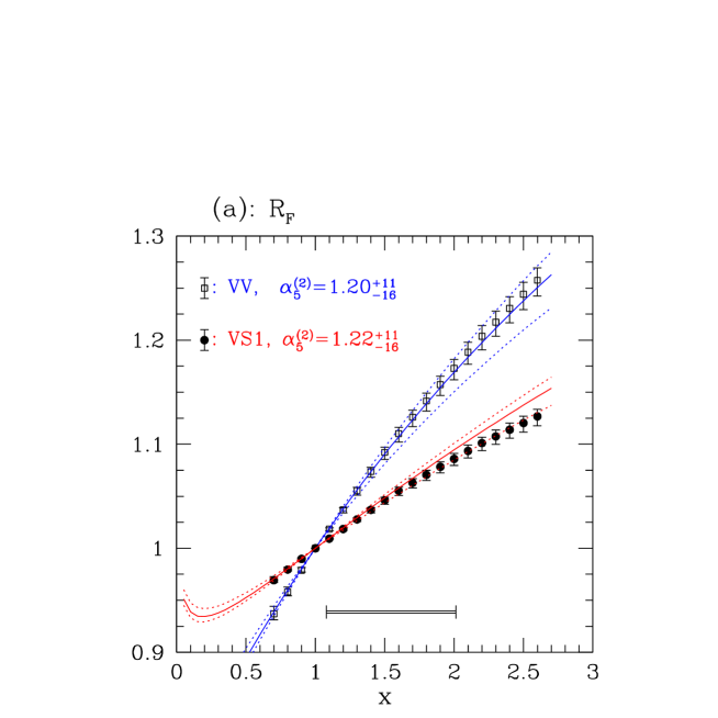
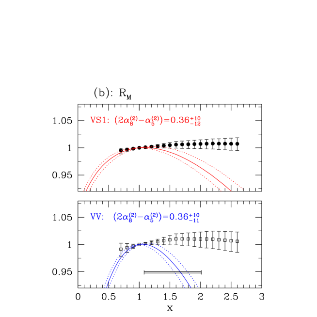
Figure 1: (a): The ratios $R_{\rm F}$ for the cases labelled “VV” and “VS1” compared with the fit to the expressions in ChPT; (b): the same for the ratios $R_{\rm M}$. Dotted lines indicate the variation due to the statistical uncertainty in the low-energy constants. The straight double lines indicate the quark mass range explored in the earlier quenched study [9].

It is striking that the data for $R_{\rm F}$ in the VV case are described remarkably well over the whole mass range, despite the fact that $\alpha_{5}^{(2)}$ has only been determined for $x\leq 1.1$. The qualitative behaviour of $R_{\rm F}$ – which features a slight curvature – is thus rather well modelled by eqs. (14) and (17), which include a linear term as well as chiral logarithms. By contrast, there are no logarithmic contributions to $R_{\rm F}$ in quenched ChPT, and the expected purely linear behaviour has indeed been observed in the data [9]. Of course, higher-order terms in the quark mass could in principle produce a curvature, and therefore these observations do not provide unambiguous evidence for chiral logarithms. Nevertheless, it is remarkable that the clear distinction between the expressions for $R_{\rm F}$ in partially quenched and quenched ChPT (i.e. the presence, respectively absence of chiral logarithms) is accompanied by corresponding qualitative differences in the numerical data.

Unlike $R_{\rm F}$ the ratio $R_{\rm M}$ is not described well for larger masses, which may signal a breakdown of the chiral expansion for this quantity for masses not much larger than $m_{\rm s}$. It is therefore conceivable that higher orders in ChPT affect the extraction of $(2\alpha_{8}^{(2)}-\alpha_{5}^{(2)})$. However, without access to quark masses that are substantially lower than our simulated ones, it is not easy to quantify reliably any uncertainty due to neglecting higher orders.

One way to examine the influence of higher orders is to extract the low-energy constants from a mass interval of fixed length, $(x_{\rm{max}}-x_{\rm{min}})=0.4$, which is then shifted inside an extended range of $0.7\leq{x}\leq 1.5$. The spread of results so obtained then serves as an estimate of the systematic errors incurred by neglecting higher orders. We note that $x=1.5$ corresponds to a quark mass slightly larger than $m_{\rm s}$. For $\alpha_{5}^{(2)}$ such a procedure yields only a small variation of $\pm 0.05$. This is not surprising, since $R_{\rm F}$ is modelled very well over the entire mass range. By contrast, the spread of results obtained for $(2\alpha_{8}^{(2)}-\alpha_{5}^{(2)})$ is as large as $\pm 0.15$. Whether or not these numbers represent realistic estimates of the actual uncertainty cannot be decided at this stage. In order to be more conservative we have decided to quote a systematic error of $\pm 0.2$ for all low-energy constants. We note that this level of uncertainty due to neglecting higher orders was also quoted in the quenched case [9], where quark masses were slightly larger.

Since we do not have enough data to extrapolate $R_{\rm F}$ and $R_{\rm M}$ to the continuum limit we also have to estimate a systematic error due to cutoff effects. As explained above, however, we expect such effects to be small. In order to get an idea of the typical size of discretisation errors we have looked again at quenched data obtained at $\beta=5.93$ [16, 17, 18] and 6.0 [9], for which the lattice spacing in physical units is roughly the same as in our dynamical simulations ($a\approx 0.1\,{\rm fm}$). For both $\beta=5.93$ and 6.0 the results for $R_{\rm M}$ and $R_{\rm F}$ are mostly consistent within errors with the corresponding values in the continuum limit (see, for instance, Fig. 1 in [9]). Furthermore, low-energy constants extracted for $a\approx 0.1\,{\rm fm}$ differ from the results in the continuum limit by less than one standard deviation. Although these findings cannot be taken over literally to the dynamical case without direct verification, they nevertheless indicate that lattice artefacts are small enough such that does not have to expect large distortions in our estimates for the low-energy constants. In order to take account of these observations we have decided to quote an additional systematic error due to lattice artefacts, which is as large as the statistical error.

Since non-perturbative estimates for the improvement coefficients $b_{\rm A}$, $b_{\rm P}$ and $c_{\rm A}$ are not available for $N_{\rm f}=2$, one may be worried that there are large uncancelled lattice artefacts of order $a$ in our data. We have addressed this issue by studying the influence of different choices for improvement coefficients on our results. To this end we have repeated the complete analysis using non-perturbative values for $c_{\rm A}$ and the combination $b_{\rm A}-b_{\rm P}$ obtained in the quenched approximation [25, 26] at a similar value of the lattice spacing, $a\approx 0.1\,{\rm fm}$. We found that the resulting variation in the estimates for $\alpha_{5}^{(2)}$ and $(2\alpha_{8}^{(2)}-\alpha_{5}^{(2)})$ is typically a factor 10 smaller than the statistical error. Thus we conclude that the influence of improvement coefficients on our results is very weak indeed.

As a final comment we point out that we have not taken finite volume effects into account in our error estimates, because different lattice sizes were not considered in our study (unlike in earlier simulations [27]). However, since $Lm_{\rm PS}=4.59$ at the reference point and $Lm_{\rm PS}=3.68$ at the lightest valence quark mass, one may not be totally convinced that such effects may be entirely neglected. We stress, though, the the definition of $R_{\rm M}$ and $R_{\rm F}$ implies that only the relative finite-size effects between hadronic quantities is relevant. Thus, as long as the mass parameter $x$ does not differ too much from unity, one can reasonably expect that finite-volume effects largely cancel in the ratios used to determine the low-energy constants. Finite-size effects in pseudoscalar masses and decay constants have also been studied in ChPT [28, 29, 30, 31]. These calculations indicate that the typical relative finite-volume effect in $m_{\rm PS}$ and $F_{\rm PS}$ between our reference point and the smallest quark mass is less than 1%.

5 Discussion and outlook

After combining the different systematic errors in quadrature we obtain as our final results in two-flavour QCD:

$$\alpha_{5}^{(2)} = 1.22\,^{+0.11}_{-0.16}\,\hbox{(stat)}\,^{+0.23}_{-0.26}\,\hbox{(syst)}$$ (35)

$$(2\alpha_{8}^{(2)}-\alpha_{5}^{(2)}) = 0.36\pm 0.10\,\hbox{(stat)}\,\pm 0.22\,\hbox{(syst)}$$ (36)

$$\alpha_{8}^{(2)} = 0.79\,^{+0.05}_{-0.07}\,\hbox{(stat)}\,\pm 0.21\,\hbox{(syst)},$$ (37)

where eqs. (35) and (36) have been combined to produce the result for $\alpha_{8}^{(2)}$.

We can now investigate the dependence of the low-energy constants on the number of dynamical quark flavours. In the quenched approximation [9] (i.e. for $N_{\rm f}=0$) it was found that

$$\alpha_{5}^{(0)} = 0.99\pm 0.06\,\hbox{(stat)}\pm 0.2\,\hbox{(syst)}$$ (38)

$$\alpha_{8}^{(0)} = 0.67\pm 0.04\,\hbox{(stat)}\pm 0.2\,\hbox{(syst)}.$$ (39)

A comparison with eq. (35) and (37) then shows that $\alpha_{5}^{(2)}$ and $\alpha_{8}^{(2)}$ are larger than their quenched counterparts by 23% and 18% respectively. We can thus conclude that the $N_{\rm f}$-dependence of the low-energy constants is fairly weak: variations between the quenched and two-flavour theories are about as large as the error due to neglecting higher orders.

Although there is a priori no reason why the weak $N_{\rm f}$-dependence should extend to the physical three-flavour case, it is still instructive to compare eqs. (35) and (37) with phenomenological values of the low-energy constants. It then becomes obvious from eqs. (2) and (7) that our results for $\alpha_{5}^{(2)}$ and $\alpha_{8}^{(2)}$ are compatible with the standard estimates found in the literature. By contrast, our numerical data for $R_{\rm F}$ and $R_{\rm M}$ suggest that a large negative value for $\alpha_{8}$, which is required for the scenario of $m_{\rm u}=0$ (see eq. (8)), is practically ruled out. Thus, provided that the quark mass behaviour in the physical three-flavour case is not fundamentally different, the possibility of a massless up-quark is strongly disfavoured.

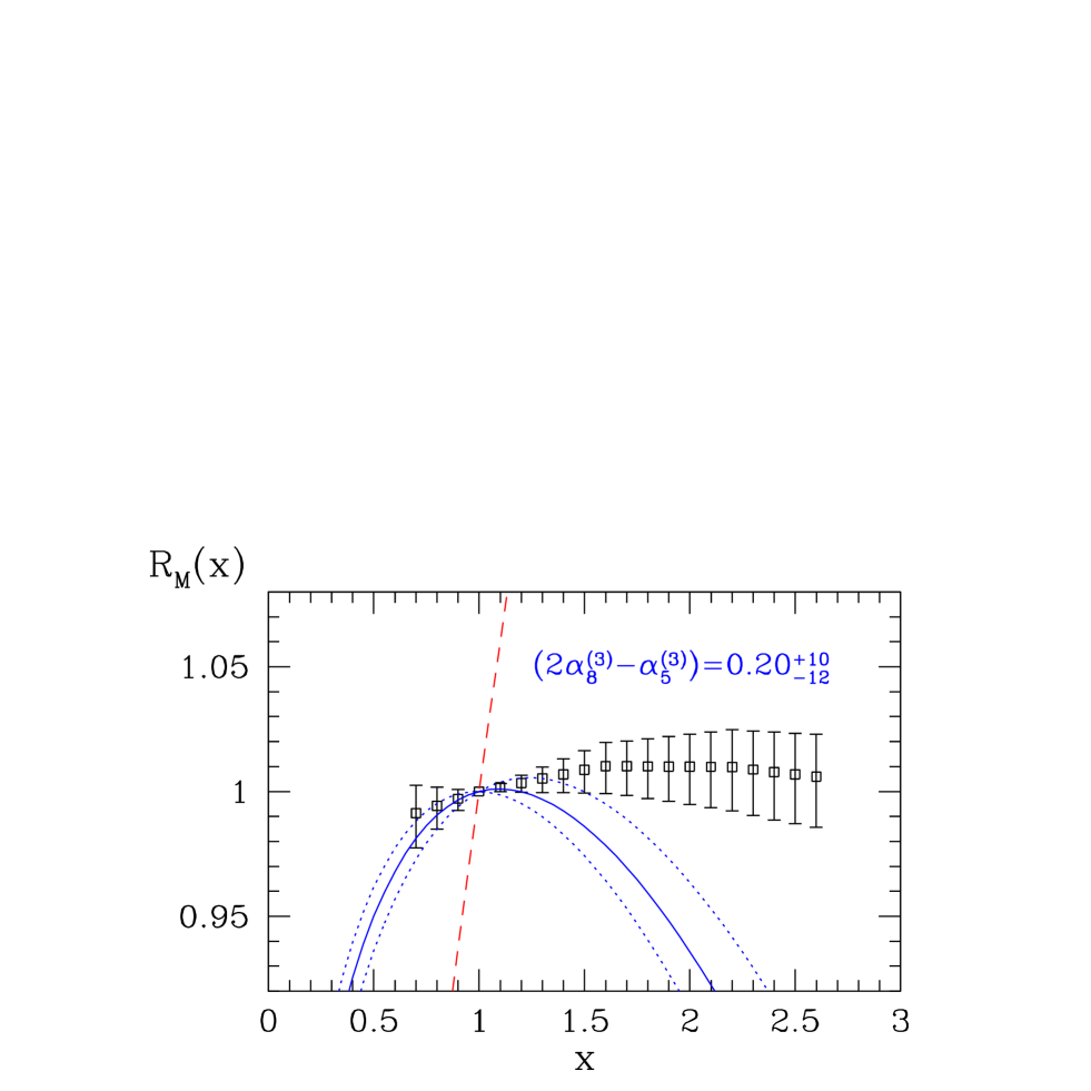
Figure 2: Data for $R_{\rm M}$ (VV case) and the curve which results if $N_{\rm f}=3$ in the determination of $(2\alpha_{8}^{(3)}-\alpha_{5}^{(3)})$ (solid line). Dotted lines represent the statistical uncertainty. The dashed curve corresponds to $(2\alpha_{8}^{(3)}-\alpha_{5}^{(3)})=-2.3$, a value which is consistent with the hypothesis of a massless up-quark.

By how much does one expect the mass dependence of $R_{\rm M}$ and $R_{\rm F}$ to differ between $N_{\rm f}=2$ and 3 ? Ultimately this must be answered by a direct simulation of the three-flavour case. For the time being we have to be content with the following gedanken simulation. Suppose that we had analysed our $N_{\rm f}=2$ data under the erroneous assumption that they had been obtained in the physical three-flavour case. We would then have set $N_{\rm f}=3$ in eqs. (14) and (17) to extract $\alpha_{5}^{(3)}$, giving $\alpha_{5}^{(3)}=0.98\raisebox{0.80002pt}{\scriptsize{$\;\begin{array}[]{@{}l@{}}\makebox[15.0pt][c]{$+$}\makebox[3.85002pt][r]{11}\\[-0.83997pt] \makebox[15.0pt][c]{$-$}\makebox[3.85002pt][r]{16}\end{array}$}}\raisebox{0.80002pt}{\scriptsize{$\;\begin{array}[]{@{}l@{}}\makebox[15.0pt][c]{$+$}\makebox[3.85002pt][r]{23}\\[-0.83997pt] \makebox[15.0pt][c]{$-$}\makebox[3.85002pt][r]{26}\end{array}$}}$. This value can be inserted into the expression for $F_{\rm K}/F_{\pi}$ in the physical theory [11], to yield

$$\frac{F_{\rm K}}{F_{\pi}}=1.247\,^{+0.009}_{-0.013}\,\hbox{(stat)}\,^{+0.019}_{-0.021}\,\hbox{(syst)},$$ (40)

which is in fair agreement with the experimental result $F_{\rm K}/F_{\pi}=1.22\pm 0.01$. This shows that the experimental value can only be reproduced if the quark mass dependence of $R_{\rm F}$ in the physical case is not much different from that encountered in our simulations for $N_{\rm f}=2$. In other words, it is reasonable to assume that the mass dependence of $R_{\rm F}$ is only weakly distorted by neglecting the dynamical quark effects due to a third flavour.

Similarly we can apply the expressions for $R_{\rm M}$ for $N_{\rm f}=3$ to our data, which gives $(2\alpha_{8}^{(3)}-\alpha_{5}^{(3)})=0.20\raisebox{0.80002pt}{\scriptsize{$\;\begin{array}[]{@{}l@{}}\makebox[15.0pt][c]{$+$}\makebox[3.85002pt][r]{10}\\[-0.83997pt] \makebox[15.0pt][c]{$-$}\makebox[3.85002pt][r]{12}\end{array}$}}\raisebox{0.80002pt}{\scriptsize{$\;\begin{array}[]{@{}l@{}}\makebox[15.0pt][c]{$+$}\makebox[3.85002pt][r]{22}\\[-0.83997pt] \makebox[15.0pt][c]{$-$}\makebox[3.85002pt][r]{23}\end{array}$}}$. The corresponding curve is shown in Fig. 2. The first-order mass correction $\Delta_{\rm M}$ is then obtained as

$$\Delta_{\rm M}=-0.04\,^{+0.05}_{-0.06}\,\hbox{(stat)}\pm 0.11\,\hbox{(syst)},$$ (41)

which is consistent with Leutwyler’s estimate (see eq. (6)). We emphasise that this does not represent a reliable result for $\Delta_{\rm M}$ derived from first principles. Nevertheless, the above discussion shows that there are examples which support the idea that the gross features of the mass dependence do not differ substantially in the two- and three-flavour cases. On the basis of this assumption one may conclude that the correction factor $\Delta_{\rm M}$ is indeed small, ruling out the scenario of a massless up-quark. As a further illustration we have included in Fig. 2 the curve which one would expect if $m_{\rm u}=0$, by taking the central values for $\alpha_{5}$ and $\alpha_{8}$ from eqs. (2) and (8).

The first priority for future work is undoubtedly the application of the method to simulations employing $N_{\rm f}=3$ flavours of dynamical quarks, and the extension of the quark mass range towards the chiral regime. While efficient simulations of QCD with odd $N_{\rm f}$ and light dynamical quarks represent an algorithmic challenge, some efforts in this direction have already been made [32]. It would also be interesting to extend applications to the case of flavour singlets, which allow a determination of $\alpha_{7}$ [8], i.e. another low-energy constant afflicted with the KM ambiguity. Methods to improve the notoriously bad signal/noise ratio in flavour-singlet correlators have been developed [33, 34], so that there are good prospects for a successful implementation.

References

- [1] T. Banks, Y. Nir and N. Seiberg, (1994), hep-ph/9403203,
- [2] H. Leutwyler, Phys. Lett. B378 (1996) 313, hep-ph/9602366,
- [3] D.B. Kaplan and A.V. Manohar, Phys. Rev. Lett. 56 (1986) 2004,
- [4] H. Leutwyler, Nucl. Phys. B337 (1990) 108,
- [5] H. Leutwyler, (1996), hep-ph/9609465,
- [6] S. Sharpe and N. Shoresh, Nucl. Phys. Proc. Suppl. 83-84 (2000) 968, hep-lat/9909090,
- [7] A.G. Cohen, D.B. Kaplan and A.E. Nelson, JHEP 11 (1999) 027, hep-lat/9909091,
- [8] S. Sharpe and N. Shoresh, Phys. Rev. D62 (2000) 094503, hep-lat/0006017,
- [9] ALPHA Collaboration, J. Heitger, R. Sommer and H. Wittig, Nucl. Phys. B588 (2000) 377, hep-lat/0006026,
- [10] J. Gasser and H. Leutwyler, Ann. Phys. 158 (1984) 142,
- [11] J. Gasser and H. Leutwyler, Nucl. Phys. B250 (1985) 465,
- [12] J. Bijnens, G. Ecker and J. Gasser, (1994), hep-ph/9411232,
- [13] ALPHA & UKQCD Collaborations, J. Garden, J. Heitger, R. Sommer and H. Wittig, Nucl. Phys. B571 (2000) 237, hep-lat/9906013,
- [14] S.R. Sharpe, Phys. Rev. D56 (1997) 7052, hep-lat/9707018,
- [15] ALPHA Collaboration, K. Jansen and R. Sommer, Nucl. Phys. B530 (1998) 185, hep-lat/9803017,
- [16] UKQCD Collaboration, J. Garden, Nucl. Phys. Proc. Suppl. 83-84 (2000) 165, hep-lat/9909066,
- [17] UKQCD Collaboration, A.C. Irving, Nucl. Phys. Proc. Suppl. 94 (2001) 242, hep-lat/0010012,
- [18] UKQCD Collaboration, C.R. Allton et al., (2001), hep-lat/0107021,
- [19] R. Sommer, Nucl. Phys. B411 (1994) 839, hep-lat/9310022,
- [20] UKQCD Collaboration, P. Lacock, A. McKerrell, C. Michael, I.M. Stopher and P.W. Stephenson, Phys. Rev. D51 (1995) 6403, hep-lat/9412079,
- [21] M. Lüscher, S. Sint, R. Sommer and P. Weisz, Nucl. Phys. B478 (1996) 365, hep-lat/9605038,
- [22] M. Lüscher and P. Weisz, Nucl. Phys. B479 (1996) 429, hep-lat/9606016,
- [23] S. Sint and P. Weisz, Nucl. Phys. B502 (1997) 251, hep-lat/9704001,
- [24] B. Efron, SIAM Review 21 (1979) 460.
- [25] M. Lüscher, S. Sint, R. Sommer, P. Weisz and U. Wolff, Nucl. Phys. B491 (1997) 323, hep-lat/9609035,
- [26] ALPHA Collaboration, M. Guagnelli et al., Nucl. Phys. B595 (2001) 44, hep-lat/0009021,
- [27] UKQCD Collaboration, C.R. Allton et al., Phys. Rev. D60 (1999) 034507, hep-lat/9808016,
- [28] J. Gasser and H. Leutwyler, Phys. Lett. 184B (1987) 83,
- [29] J. Gasser and H. Leutwyler, Phys. Lett. 188B (1987) 477,
- [30] C.W. Bernard and M.F.L. Golterman, Phys. Rev. D46 (1992) 853, hep-lat/9204007,
- [31] S.R. Sharpe, Phys. Rev. D46 (1992) 3146, hep-lat/9205020,
- [32] C. Bernard et al., (2001), hep-lat/0104002,
- [33] UKQCD Collaboration, C. McNeile and C. Michael, Phys. Lett. B491 (2000) 123, hep-lat/0006020,
- [34] UKQCD Collaboration, C. McNeile and C. Michael, Phys. Rev. D63 (2001) 114503, hep-lat/0010019,