New Cosmological and Experimental Constraints on the CMSSM
Abstract:
We analyze the implications of several recent cosmological and experimental measurements for the mass spectra of the Constrained MSSM (CMSSM). We compute the relic abundance of the neutralino and compare the new cosmologically expected and excluded mass ranges with those ruled out by the final LEP bounds on the lightest chargino and Higgs masses, with those excluded by current experimental values of , and with those favored by the recent measurement of the anomalous magnetic moment of the muon. We find that for there remains relatively little room for the mass spectra to be consistent with the interplay of the several constraints. On the other hand, at larger values of the decreasing mass of the pseudoscalar Higgs gives rise to a wide resonance in the neutralino WIMP pair-annihilation, whose position depends on the ratio of top and bottom quark masses. As a consequence, the cosmologically expected regions consistent with other constraints often grow significantly and generally shift towards superpartner masses in the TeV range.
1 Introduction
Cosmology provides an important restriction on otherwise allowed supersymmetric mass spectra. This in particular is the case with the relic density of the lightest supersymmetric particle (LSP) which, in the presence of -parity, is stable. A natural candidate for the LSP is the lightest neutralino . Its relic abundance has been a subject of a large volume of papers [1], starting from Refs. [2, 3] up to the recent comprehensive studies [4, 5, 6, 7]. It is well known that can vary over several orders of magnitude but that it is also often consistent with the abundance of non-baryonic cold dark matter (CDM) in the Universe whose determinations have been improving steadily. Recent reviews give more narrow ranges for the components (matter and baryonic ) of the Universe and the Hubble parameter than in the past. For example, for the matter component in Ref. [8] one finds which is consistent with of Ref. [9] and of Ref. [10]. The baryonic component is now [8, 9, 10] while the Hubble parameter is [8] ( [9]). Based on this, and assuming that the neutralino LSP makes up the dominant component of the CDM in the Universe, we now select the range of the neutralino relic abundance
| (1) |
as conservatively matching the recent observations. Furthermore, we put an upper bound
| (2) |
based solely on the constraints on the age of the Universe. These ranges will also allow a comparison with the favored values of in the range which have often been used in the recent literature.
The latest determinations of from the measurements of the CMBR, based on assuming reasonable ranges for other cosmological parameters (priors), like , etc, give [11, 12], or, assuming more priors, even much smaller errors: [12]. We do not feel yet ready to accept these narrow ranges as robust enough for our analysis. In particular, we note that, assuming , the DASI analysis [11] finds which implies . Likewise, the most recent ROSAT measurement gives [13] which again allows for larger values of . Nevertheless, below we will discuss the impact on our results of assuming, after subtracting the baryonic component, that is in the range and .
Cosmological constraints (1)–(2) have a particularly strong effect in the framework of the Constrained MSSM (CMSSM) [14, 15]. In the CMSSM, in addition to the requirement of a common gaugino mass at the unification scale , which is usually made in the more generic Minimal Supersymmetric Standard Model (MSSM), one further assumes that the soft masses of all scalars (sfermion and Higgs) are equal to at , and analogously that the trilinear soft terms unify at at some common value . These parameters are run using their respective Renormalization Group Equations (RGEs) from to some appropriately chosen low-energy scale where the Higgs potential (including full one-loop corrections) is minimized while keeping the usual ratio of the Higgs VEVs fixed. The Higgs/higgsino mass parameter and the bilinear soft mass term are next computed from the conditions of radiative electroweak symmetry breaking (EWSB), and so are the Higgs and superpartner masses. The CMSSM thus has a priori only the usual
| (3) |
as input parameters. (A comprehensive set of formulae that we will refer to can be found for example in Ref. [16].) However, in the case of large and/or large some resulting masses will in general be highly sensitive to the assumed physical masses of the top and the bottom (as well as the tau) [4] but they will also strongly depend on the correct choice of the scale . This in particular will affect the impact of the cosmological constraints (1)–(2) as we will discuss below.
In the CMSSM, the LSP neutralino is often a nearly pure bino [17, 18, 15] because the requirement of radiative EWSB typically gives where is the soft mass of the bino. This often (albeit not always! [15]) allows one to impose strong constraints from on and (and therefore also on heaviest Higgs and superpartner masses) in the ballpark of . This was originally shown in Refs. [18, 15] and later confirmed by many subsequent studies starting from [19] up to the most recent analyses [4, 5, 20, 7].
2 Experimental Constraints
In the case of the CMSSM, the most important experimental constraints from LEP are those on the masses of the lightest chargino and Higgs boson . For the first one we adopt the bound since the actual limits from the LEP experiments are very close to this value. The lightest Higgs mass has been a subject of much debate on both the experimental [21] and the theory side. The termination of LEP has left the first one unresolved for at least a few years. On the theory front, due to large radiative corrections, the precise value of still remains somewhat dependent on the procedure of computing it [22, 23, 24, 25]. In our analysis we will conservatively assume but will keep in mind that the theoretical uncertainty in in the CMSSM is probably of the order of –.
Non-accelerator experimental results are also of much importance. First, there has been much recent activity in determining . A recent combined experimental result [26]111The most recent update [34], which incorporates the new CLEO result [27], gives . As we will coment again later, adopting this new data would exclude somewhat larger regions of the CMSSM parameter space. allows for some, but not much, room for contributions from SUSY when one compares it with the updated prediction for the Standard Model (SM) [26]. Second, at large next-to-leading order supersymmetric corrections to become important [28, 29, 30, 31, 32, 33]. In our analysis we adopt the full expressions for the dominant terms derived in Ref. [33]. We also include the -quark mass effect on the SM value which was subsequently pointed out in Ref. [34]. We add the two errors (the experimental and SM) in quadrature and further add linearly to accommodate the theoretical uncertainty in SUSY contributions which is roughly of the SM value for branching ratio [35]. Altogether we conservatively allow our results to be in the range for SM plus two-Higgs doublets plus superpartner contribution. The excluded regions of SUSY masses will not however be extremely sensitive to the choice of these error bars.
Lastly, much excitement has recently been caused by the first measurement by the Brookhaven experiment E821 of the anomalous magnetic moment of the muon [36]. Taken at face value, the result implies a discrepancy between the experimental value and the SM prediction . There is much ongoing debate about improving the understanding of the precise contribution from the SM, as has been reported for example in Ref. [37]. In particular, there has been a tendency of moving the SM prediction towards the range of experimental values [38]. In our analysis we will use the published results to allow SUSY contributions in the ranges () and () but will comment on the effect of varying these numbers later. Here we only note that we consider the upper limit on (which implies a lower limit on and ) as rather robust. In contrast, the lower limit on (and the resulting upper limit on and ) should be approached with much caution. We will comment on this further when we present our results.
3 Procedure
We calculate superpartner and Higgs mass spectra using the package ISASUGRA (v.7.51) but make some important modifications which will be described below. We refer the reader to Ref. [39] for a more detailed description of the code. Here we will only highlight the main points of the procedure. The overall strategy is to first find an approximate spectrum of the Higgs and SUSY masses and then iterate the procedure of running the RGEs between and the low scale until a satisfactory consistency is achieved. In the initial step one runs the two-loop RGEs for the gauge couplings up and identifies as the point where and are equal. Exact unification of with the other two SM gauge couplings is not assumed as it would predict a value far too large compared with the experimental range [40] which we take as input.
The top, bottom and tau masses must also be treated with care since their assumed values often have an important effect on the running of the RGEs, especially at large . The pole mass of the top [40] is initially converted to the running mass in the scheme using a two-loop QCD correction with running computed at three loops, and is then identified with in the scheme. In subsequent iterations, once SUSY masses have been computed, also one-loop SUSY corrections from squark and gluino contributions are included to give .
As regards the mass of the bottom, the Particle Data Book [40] quotes the range – for the running mass in the scheme . We adopt the similar range [41] which has been used in other recent analyses [4, 5]. In ISASUGRA is initially run up to using a one-loop QCD+QED formula, with running computed at three loops and at one loop, to obtain which is assumed to be the same as in the -scheme. In subsequent steps, once the SUSY masses have been computed, one includes SUSY corrections [28, 42] from squark/gluino and squark/chargino loops which become important at large
| (4) |
where is computed in the initial step and stands for a SUSY mass correction. (We note that in ISASUGRA it is the pole mass that is used as an independent parameter and is actually ‘hardwired’ at [and in some routines at ]. We have modified the package to allow it to treat as an external parameter which is then adjusted to match the desired value for . The conversion between the two is done using a one-loop expression.)
Finally, the pole mass of the -lepton is now well measured [40]. It is converted to the scheme in SUSY using an analogous procedure to the bottom mass. In particular, a threshold due to is added and one-loop SUSY corrections due to just chargino exchange are included after the initial step.
At the initial values of and are used to compute the corresponding Yukawa couplings and for a fixed value of . The Yukawa coupling of the top is computed at . These couplings are next run up to using two-loop RGEs in the scheme with the same initial mass threshold as for the gauge couplings, but are not assumed to unify.
In the second step, starting from , for a given choice of , , , and , the RGEs for the masses and couplings are run down to the low scale. Here much attention is paid to extracting the parameters at a right energy scale . The RGEs for the gaugino masses are run down until reaches their respective running values and analogously for the sfermion soft masses and the third-generation trilinear parameters , and . The top Yukawa RGE is run down to while the RGEs for the other two Yukawa couplings of the third generation are run down to .
Of particular importance is a correct treatment of the Higgs sector and the conditions for the EWSB. This is because of the spurious but nagging -scale dependence of the scheme [44]. Even including full one-loop corrections to the Higgs potential is not sufficient to significantly reduce the scale dependence when one minimizes the Higgs potential at the scale . Instead, it has been argued, for example in [45], that the scale dependence is significantly reduced by evaluating the (one-loop corrected) Higgs potential at with () denoting the physical masses of the stops. This is because, at this scale, the role of the otherwise large log-terms from the dominant stop-loops will be reduced. Here we follow this choice which is also adopted in ISASUGRA. (Actually, in ISASUGRA a very similar prescription is used with , where () denote the soft masses of the stops, but we do not think that this difference is of much importance). At this scale one evaluates the conditions for the EWSB which determine as well as the bilinear soft mass parameter
| (5) | |||||
| (6) |
where are the squares of the soft mass terms of the Higgs doublets and are their respective one-loop corrections.
In the package ISASUGRA only the (dominant) third-generation (s)fermion one-loop corrections were included. We have added all the one-loop corrections following Ref. [42], in particular the chargino and neutralino ones. It has been claimed in Ref. [43] that, while normally subdominant, these can contribute to increasing at large and large .
The mass of the pseudoscalar will play a crucial role in computing , especially at very large . This is so for three reasons: becomes now much smaller [49] than at smaller due to the increased role of the bottom Yukawa coupling; because the -resonance in is dominant since the coupling for down-type fermions; and because, in contrast to the heavy scalar , this channel is not -wave suppressed [1]. In ISASUGRA is computed as
| (7) |
where stands for the full one-loop corrections which can be significant [42].
The neutralino relic density can be reliably computed both away from resonances and new final-state thresholds, where the usual expansion in powers of (where is the temperature) works well, as well as in the vicinity of such special points. Exact analytic cross sections, which will soon become available [46], allow us to consistently and precisely determine both near and away from such special points by solving the Boltzmann equation as in Ref. [47, 48]. (In the case of the expansion, analytic formulae for the thermally-averaged product of the annihilation cross section and the relative velocity are given in Refs. [49, 1] and are applicable far away from resonances and thresholds. However, caution is advised in combining them with a numerical integration of exact cross sections in the vicinity of the resonances. This is because one then usually neglects interference terms which can play some role. Furthermore, the range of around the pseudoscalar resonance where the expansion fails badly can be as large as several tens of GeV [50].)
We also include the co-annihilation with next-to-lightest SUSY particles (NLSPs) which in some cases is important. The co-annihilation with the lightest chargino and the next-to-lightest neutralino is treated without any approximation following Refs. [51, 48]. In the CMSSM, the lighter stau () is the LSP in the region [15] and just above the boundary the neutralino LSP can efficiently co-annihilate with it and with the other sleptons [52]. In this analysis we use the approximate expressions given in the second paper of Ref. [52] even though they do not include the effects of , of the mixing, in some channels of the mass of the , etc [4], which make them less reliable at large [4]. We have made an attempt at improving the available formulae by including in the propagators the widths of the gauge and Higgs bosons and the neutralinos, which otherwise become singular. Furthermore, ISASUGRA does not include one-loop corrections to the neutralino, chargino and slepton masses which can be of the order of a few per cent [42]. This will have a comparable effect on the exact position of the boundary between the neutralino and the LSP especially at large . For these reasons we will treat our numerical results in the co-annihilation region as somewhat less reliable but would not expect any major changes if the mentioned effects were included.
4 Results
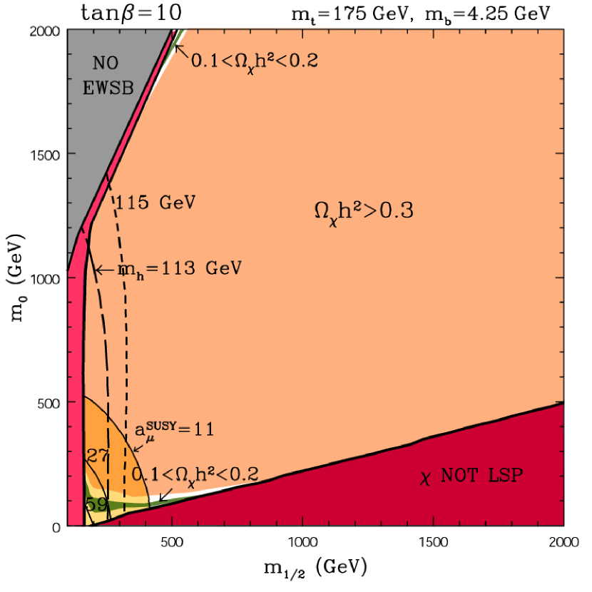
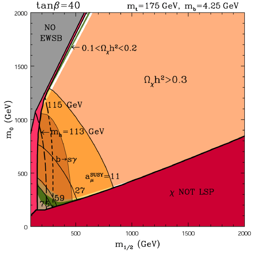
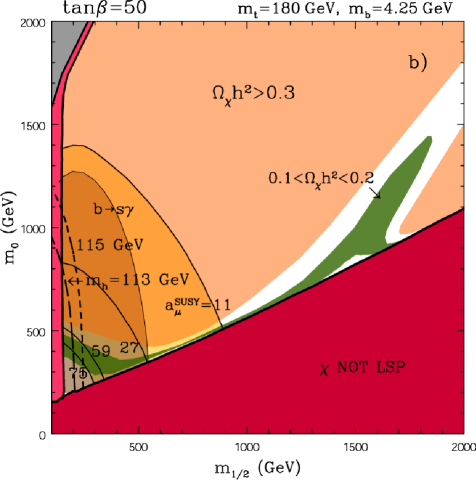
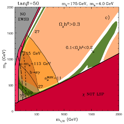
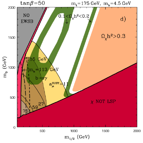
We present our results in the plane () for several representative choices of and other relevant parameters as specified below. First, in Figs. 1–3 we show the experimental and cosmological bounds for respectively and and for , and the central values of and . In Figs. 1 and 2 we can see many familiar features. At there is a (dark red) wedge where the is the LSP. On the other side, at we find large (grey) regions where the EWSB is not achieved. Just below the region of no-EWSB the parameter is small but positive which allows one to exclude a further (light red) band by imposing the LEP chargino mass bound. As one moves away from the wedge of no-EWSB, increases rapidly. That implies that, just below the boundary of the no-EWSB region, the LSP neutralino is higgsino-like but, as one moves away from it, it very quickly becomes the usual nearly pure bino. This causes the relic abundance to accordingly increase rapidly from very small values typical for higgsinos in the hundred GeV range, through the narrow strip () of the cosmologically expected (green) range (1) to much larger values, excluded (light orange) by (2). In particular, in the whole region allowed by the chargino mass bound the LSP is mostly bino-like. We remind the reader that in the nearly pure bino case the neutralino mass is given by [53].
It is clear from Figs. 1 and 2 that up until the overall shape of the cosmologically expected (1) and excluded (2) regions does not change much. Generally one finds a robust (green) region of expected at in the range of a few hundred GeV [15]. In addition, at , just above the wedge where the LSP is the , the co-annihilation of the neutralino LSP with opens up a very long and very narrow strip which is allowed by the bounds (1)–(2). Finally, as mentioned above, at , very close to the region of no-EWSB, again one finds a very narrow range of consistent with (1). A closer examination would be required to establish to what extent this region of and overlaps with that corresponding to ‘focus points’ advocated in Ref. [20].
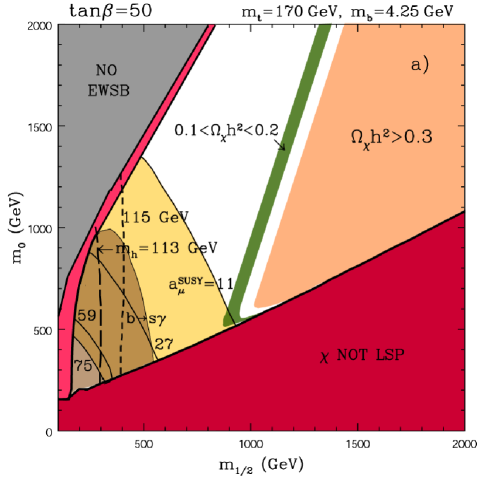
The region of no-EWSB is quite sensitive to the relative values of the top and bottom masses. Generally, at fixed , increasing (decreasing) the top mass relative to the bottom mass causes the region of no-EWSB to move up (down) considerably because of the diminishing (growing) effect of the bottom Yukawa coupling on the loop correction to the conditions of EWSB (5)–(6). This effect can be explicitly seen in Fig. 4a and b but it remains basically true also for much smaller . At fixed top and bottom masses, as decreases, the region of no-EWSB moves towards somewhat larger values of and smaller values of but the overall effect is not very significant.
The lightest Higgs mass also grows with as expected. In the Figures we plot the contours of (which, within the uncertainties mentioned earlier, corresponds to the LEP lower limit) and of where an intriguing possibility of a Higgs signal has been reported [21]. Larger values of are given by contours which are shifted along the axis with roughly equal spacings but diverge somewhat at larger . We remind the reader that the values of that we plot have been obtained using ISASUGRA. When we use FeynHiggsFast [25], we obtain values lower by , as can be seen from Table 1.
Other constraints behave with increasing as expected. In particular, the (light brown) region excluded by grows significantly because the dominant chargino-squark contribution to the branching ratio grows linearly with . On the other hand, the excluded region does not change much as we vary the assumed lower bound on . Taking the (slightly higher) most recent range (see Section 2) enlarges the excluded regions of the ()–plane by some additional .
As for the SUSY contribution to the anomalous magnetic moment of the muon, the , and especially , (yellow) range of allowed becomes significantly enlarged towards larger and because the dominant sneutrino-chargino loop exchange contribution grows with [54]. It is clear that the dependence of on and is relatively weak and therefore, in our opinion, no robust upper bound on superpartner masses can at present be placed. On the other hand, the low ranges of and below the lines corresponding to the upper () limits on , respectively, are probably firmly excluded but are not too big.
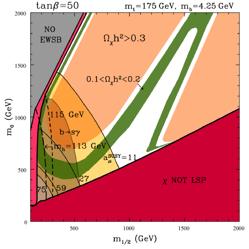
The region of very large deserves a separate discussion. First, as can be seen by comparing Figs. 1 and 2, we find relatively little variation in the overall shape of the constraints as increases up to . However, as grows, above a new important feature appears which is prominently reflected in the neutralino relic abundance, as can be seen from Figs. 3 and 4. The heavy Higgs bosons become ‘light’ enough [49, 19, 53, 55] to “enter the ()–plane from the right” and cause a significant decrease in , predominantly through a very wide -resonance. Clearly, unlike for smaller values of , there is now much variation in the position of the -resonance and accordingly in the shape of the allowed and excluded regions of as one varies and/or . Generally, as increases relative to , the position of the resonance moves to the left and the shapes of the regions where is in the prefered range (1) and is excluded by (2) change accordingly. Qualitatively this behavior again clearly demonstrates the growing impact of at large . More quantitatively, one can see why this happens by examining Eq. (7) where the one-loop correction [16] to from the sbottoms grows with as .
The white regions to the left of the green regions of , as well as around the green ‘island’ in Fig. 4d, correspond to . The white areas between the favored green regions and the excluded light orange range () as well as the white pocket inside the green region in Fig. 4d correspond to . One should also mention that, in contrast to much smaller , at large , does not grow rapidly with increasing superpartner masses but instead changes very gradually and does not exceed unity by more than a factor of a few. This is again mostly caused by the very wide -resonance because the -width is large and actually growing with as well as and . As one cuts along the axis at fixed in Figs. 3 and 4, one can see that first grows somewhat, then gradually decreases around the -resonance and then increases again at large .
The most recent measurements of and have now implied much more restrictive ranges and , as discussed earlier. We do not show these ranges in our Figures but can easily summarize their effect. The range corresponds roughly to the half of the allowed green strips (when cutting along them) on the side of the axes and the origin. In Fig. 4d this corresponds to the the outer halfs of the green ‘island’. Requiring causes a further shrinking of the green regions in the same direction by roughly another factor of two.
Clearly, as increases above , the cosmologically expected and excluded regions are gradually shifted towards larger and thus significantly relaxing the tight bounds characteristic of smaller . This is especially true when the top-to-bottom mass ratio is on the lower side. Overall, however, cosmological constraints on now permit much larger superpartner masses than at smaller , and not only in the very narrow strips close to the regions of no-EWSB and/or -LSP.
The case of very large is obviously quite complicated. We are not even convinced that ISASUGRA and other currently available codes for generating SUSY mass spectra are fully reliable at such large values of , especially in the regime of . First, two-loop corrections to the effective potential would need to be added to ensure a further reduction of the scale dependence. Second, now the Yukawa couplings of the bottom and the tau become comparable with that of the top and the contribution to the effective potential from the sbottom and stau loops becomes of the same order as that from the stops. This introduces at least two more mass scales and the choice of the right scale for minimizing the Higgs potential becomes much more complicated. The variation in the shape and position of the region of no-EWSB and the heavy Higgs masses with and that we discussed above is, in our opinion, probably just a reflection of the above problems.
One may conclude that, given the technical difficulty involved, the available codes for computing especially and the heavy Higgs masses are not yet fully applicable to such large values of , especially for and we applaud the ongoing efforts to ameliorate the situation [56].
On the other hand, the case of is an intriguing one as it corresponds to the infrared quasi-fixed point solution of the top Yukawa coupling for the Yukawa RGEs when the approximate unification with and is further assumed [57, 58, 59]. Additionally, in –based models various texture models for mass matrices of leptons and quarks invariably require large [60, 61]. Collider phenomenology can also be distinctively different [62] with the usual multilepton signatures for SUSY signals now being much reduced, although new signals may appear involving -leptons and -quarks in the final state.
Finally, in Table 1 we present several representative cases consistent with all experimental and cosmological bounds. All the mass parameters are given in GeV. The Table should be helpful in a more detailed comparison of our results with other groups.
| Case | RRN1 | RRN2 | RRN3 | RRN4 | RRN5 | RRN6 | RRN7 |
|---|---|---|---|---|---|---|---|
| 10 | 10 | 40 | 45 | 50 | 50 | 50 | |
| 300 | 500 | 250 | 600 | 700 | 280 | 1000 | |
| 75 | 1900 | 1225 | 350 | 600 | 1250 | 1000 | |
| 175 | 175 | 175 | 175 | 175 | 175 | 175 | |
| 4.25 | 4.25 | 4.25 | 4.25 | 4.25 | 4.25 | 4.25 | |
| -556.3 | -886.8 | -453.8 | -1028 | -1184 | -495.3 | -1644 | |
| -803.5 | -1245 | -573.5 | -1274 | -1412 | -579.2 | -1937 | |
| -186.0 | -301.5 | -74.2 | -166.5 | -143.0 | -38.4 | -219.6 | |
| (ISA) | 114.6 | 118.0 | 115.5 | 120.0 | 120.7 | 115.8 | 122.3 |
| (FHF) | 112.8 | 115.1 | 113.1 | 118.3 | 119.0 | 113.5 | 120.5 |
| 443.6 | 1920 | 833.6 | 601.9 | 652.5 | 537 | 917.5 | |
| 397.3 | 299.4 | 166.7 | 701.5 | 785.2 | 209.5 | 1038 | |
| 117.5 | 196.6 | 87.8 | 247.9 | 291.7 | 105.3 | 424.6 | |
| 215.5 | 272.7 | 129.6 | 461.1 | 542.4 | 163.7 | 784.6 | |
| 706.3 | 1224 | 659.5 | 1333 | 1558 | 727.9 | 2176 | |
| 221.0 | 1919 | 1231 | 515.9 | 757.2 | 1258 | 1193 | |
| 140.9 | 1905 | 1227 | 394.8 | 653.2 | 1253 | 1064 | |
| 132.2 | 1889 | 1035 | 254.4 | 429.6 | 911.0 | 734.1 | |
| 224.4 | 1911 | 1140 | 503.1 | 695.6 | 1104 | 1075 | |
| 630.0 | 2085 | 1294 | 1219 | 1477 | 1341 | 2118 | |
| 608.9 | 2075 | 1293 | 1180 | 1434 | 1337 | 2049 | |
| 634.9 | 2087 | 1296 | 1221 | 1479 | 1343 | 2120 | |
| 607.8 | 2074 | 1293 | 1175 | 1428 | 1337 | 2041 | |
| 468.3 | 1398 | 835.8 | 948.0 | 1139 | 870.0 | 1634 | |
| 651.9 | 1780 | 1021 | 1137 | 1335 | 1020 | 1869 | |
| 580.3 | 1780 | 1003 | 1049 | 1255 | 996.5 | 1806 | |
| 609.6 | 2059 | 1135 | 1123 | 1331 | 1093 | 1877 | |
| 3.4 | 3.6 | 2.8 | 2.6 | 2.8 | 2.6 | 3.0 | |
| 20.5 | 1.1 | 12.0 | 21.8 | 15.0 | 14.4 | 7.0 | |
| 0.17 | 0.20 | 0.16 | 0.14 | 0.13 | 0.17 | 0.16 |
Our results show a sizeable difference at large when compared with some other recent analyses [63, 4, 5]. First, in Ref. [63] a similar procedure for computing Higgs and SUSY mass spectra was used as in our modified version of ISASUGRA, which was based on Ref. [42]. In Ref. [63] somewhat different quark input masses were used ( and ) but, even for that choice, we find that our version of ISASUGRA still produced significantly lower values for (by some ) at large than in Ref. [63], which we find somewhat puzzling. (This affects the position of the -resonance and therefore also the relic density contours, even though in Ref. [63] the latter was computed only in an approximate way using the package NEUTDRIVER.) As regards Refs. [4, 5], we find a sizeable discrepancy especially in the mass of the heavy Higgs bosons (especially the pseudoscalar) and therefore also in the position of the -resonance. We believe that our computation of , especially near the -resonance, is somewhat more precise due to our exact treatment of the -annihilation. However, we are convinced that the main difference comes from the fact that in Refs. [4, 5] the effective Higgs potential was minimized at the scale [64] while in ISASUGRA this is done at as discussed in Sect. 3. This leads to large differences in the values of and especially at larger and which were also discussed in Ref. [64]. We have checked numerically that choosing the minimization scale at typically gives significantly smaller mass of the pseudoscalar for a given choice of other parameters. This has a strong effect on the location of its resonance in the ()–plane and therefore on the neutralino relic abundance. It also strongly affects the position of the region of no-EWSB.
5 Summary
In summary, the interplay of the different experimental constraints and the cosmologically expected (1) and allowed (2) regions shows a significant dependence on . Generally, the region excluded by grows with and so does the region favored by the recent measurement of the anomalous magnetic moment of the muon. The lightest Higgs mass limit gives a lower bound on , which however becomes weaker as and/or grow. Additionally, there still remains some theoretical uncertainty in computing , of the order of –. As can be seen by comparing the contours of 113 and , this affects the range of excluded by several tens of GeV at larger and even by nearly hundred GeV at smaller .
At , the experimental bounds exclude large parts of the generic ‘low-mass’ region of both and (below a few hundred GeV [15]) of the expected (green) range of the neutralino relic abundance () which itself is strongly squeezed by the conservative upper bound . What remains are the two narrow bands of expected along the wedges of no-EWSB and -LSP of which the second is (slightly) more favored by the measurement of .
The picture changes dramatically as approaches . The cosmologically expected regions expand significantly both in size and towards larger and . They also become further affected by the appearance of the resonance due to the pseudoscalar, whose mass decreases significantly at very large , and especially for smaller values of the ratio of the top to bottom masses. Overall, it is clear that, in contrast to smaller values of , at such large cosmological constraints point towards significantly larger gluino and/or sfermion masses in the TeV range.
NOTE ADDED: After our analysis was completed, we became aware of Ref. [7] where the impact on the CMSSM of the recent highly restrictive determination of [12] was discussed, along with other constraints, except for , for the choice and [65]. We find a reasonable agreement in the overlapping results, in particular in the location of the resonance of the pseudoscalar . Similarly, we find a reasonable agreement with Refs. [66, 67] which were completed after our paper.
Acknowledgments.
LR and RRdA would like to thank P. Gambino and G. Giudice for beneficial discussions regarding large corrections to . LR further acknowledges conversations with B. Allanach, J. Ellis, W. Hollik, K. Matchev, P. Nath, K. Olive, F. Paige, M. Quiros, S. Raby, D. Tovey, G. Weiglein as well as the combined ‘unnamed physicist’ for providing useful comments on various aspects of the analysis.References
- [1] For a review see G. Jungman, M. Kamionkowski and K. Griest, Phys. Rept. 267 (195) 1996.
- [2] H. Goldberg, Phys. Rev. Lett. 50 (1419) 1983.
- [3] J. Ellis, J.S. Hagelin, D.V. Nanopoulos, K.A. Olive and M. Srednicki, Nucl. Phys. B 238 (453) 1984.
- [4] J. Ellis, T. Falk, G. Ganis, K.A. Olive and M. Srednicki, Phys. Lett. B 510 (236) 2001.
- [5] J. Ellis, D.V. Nanopoulos and K.A. Olive, Phys. Lett. B 508 (65) 2001.
- [6] R. Arnowitt, B. Dutta and Y. Santoso, Nucl. Phys. B 606 (59) 2001; R. Arnowitt, B. Dutta, B. Hu and Y. Santoso, Phys. Lett. B 505 (177) 2001.
- [7] V. Barger and C. Kao, hep-ph/0106189.
- [8] M.S. Turner, astro-ph/0106035.
- [9] J.R. Primack, astro-ph/0007187.
- [10] L. Krauss, astro-ph/0106149.
- [11] C. Pryke, et al., The DASI Collaboration, astro-ph/0104490.
- [12] C.B. Netterfield, et al., The BOOMERanG Collaboration, astro-ph/0011378.
- [13] S. Borgani, et al., The ROSAT Collaboration, astro-ph/0106428.
- [14] For a review see, for instance, H.P. Nilles, Phys. Rept. 110 (1) 1984.
- [15] G.L. Kane, C. Kolda, L. Roszkowski, and J.D. Wells, Phys. Rev. D 49 (6173) 1994.
- [16] V. Barger, C.E.M. Wagner, et al., Report of the SUGRA Working Group for Run II of the Tevatron, hep-ph/0003154.
- [17] P. Nath and R. Arnowitt, Phys. Rev. Lett. 70 (3696) 1993.
- [18] R.G. Roberts and L. Roszkowski, Phys. Lett. B 309 (329) 1993.
- [19] H. Baer and M. Brhlik, Phys. Rev. D 53 (597) 1996; H. Baer, M. Brhlik, M.A. Diaz, J. Ferrandis, P. Mercadante, P. Quintana and X. Tata, Phys. Rev. D 63 (015007) 2001.
- [20] J. L. Feng, K. T. Matchev and T. Moroi, Phys. Rev. Lett. 84 (2322) 2000, hep-ph/9908309 and Phys. Rev. D 61 (075005) 2000, hep-ph/9909334.
-
[21]
R. Barate et al.(ALEPH), Phys. Lett. B 495 (1) 2000, hep-ex/0011045;
P. Abreu et al.(DELPHI), Phys. Lett. B 499 (23) 2001, hep-ex/0102036;
M. Acciarri et al., (L3), Phys. Lett. B 495 (18) 2000, hep-ex/0011043;
G. Abbiendi et al., (OPAL), Phys. Lett. B 499 (38) 2001, hep-ex/0101014. - [22] M. Carena, J.R. Espinosa, M. Quiros and C.E.M. Wagner, Phys. Lett. B 355 (209) 1995, hep-ph/9504316; M. Carena, M. Quiros and C.E.M. Wagner, Nucl. Phys. B 461 (407) 1996, hep-ph/9508343.
- [23] J.R. Espinosa and R.-J. Zhang, hep-ph/9912236 and hep-ph/0003246.
- [24] M. Carena, et al., Nucl. Phys. B 580 (29) 2000, hep-ph/0001002.
- [25] S. Heinemeyer, W. Hollik and G. Weiglein, hep-ph/0002213.
- [26] M. Misiak, talk at the XXXVIth Rencontres de Moriond, Les Arcs, March 2001, hep-ph/0105312.
- [27] S. Chen, et al., The CLEO Collaboration, hep-ex/0108032.
- [28] L.J. Hall, R. Rattazzi and U. Sarid, Phys. Rev. D 50 (7048) 1994, hep-ph/9306309.
- [29] H. Baer and M. Brhlik, Phys. Rev. D 58 (015007) 1998, hep-ph/9712305.
- [30] T. Blazek and S. Raby, Phys. Rev. D 59 (095002) 1999, hep-ph/9712257.
- [31] W. de Boer, et al., hep-ph/0007078 and hep-ph/0102163.
- [32] M. Carena, D. Garcia, U. Nierste and C.E.M. Wagner, Phys. Lett. B 499 (141) 2001.
- [33] G. Degrassi, P. Gambino and G.F. Giudice, J. High Energy Phys. 0012 (009) 2000.
- [34] P. Gambino and M. Misiak, hep-ph/0104034.
- [35] P. Gambino, private communication.
- [36] H. N. Brown, et al., The Muon () Collaboration, hep-ex/0102017.
- [37] A. Czarnecki, talk at the XXXVIth Rencontres de Moriond, Les Arcs, March 2001.
- [38] See Ref. [37] and, for example, S. Narison, hep-ph/0103199.
- [39] H. Baer, F.E. Paige, S.D. Protopopescu and X. Tata, hep-ph/0001086.
- [40] D.E. Groom, et al., Eur. Phys. J. C 15 (1) 2000, http://pdg.lbl.gov/.
- [41] G. Martinelli and C.T. Sachrajda, Nucl. Phys. B 559 (429) 1999; C.T. Sachrajda, hep-lat/0101003.
- [42] D.M. Pierce, J.A. Bagger, K. Matchev and R. Zhang, Nucl. Phys. B 491 (3) 1997.
- [43] A. Katsikatsou, A.B. Lahanas, D.V. Nanopoulos and V.C. Spanos, Phys. Lett. B 501 (2001) 69.
- [44] G. Gamberini, G. Ridolfi and F. Zwirner, Nucl. Phys. B 331 (331) 1990.
- [45] B. de Carlos and J.A. Casas, Phys. Lett. B 309 (320) 1993.
- [46] T. Nihei, L. Roszkowski and R. Ruiz de Austri, in preparation.
- [47] P. Gondolo and G. Gelmini, Nucl. Phys. B 360 (145) 1991.
- [48] P. Gondolo et. al., astro-ph/0012234.
- [49] M. Drees and M. Nojiri, Phys. Rev. D 47 (376) 1993.
- [50] T. Nihei, L. Roszkowski and R. Ruiz de Austri, J. High Energy Phys. 0105 (063) 2001.
- [51] J. Edsjo and P. Gondolo, Phys. Rev. D 56 (1879) 1997.
- [52] J. Ellis, T. Falk and K.A. Olive, Phys. Lett. B 444 (367) 1998; J. Ellis, T. Falk, K.A. Olive and M. Srednicki, Astropart. Phys. 13 (181) 2000.
- [53] V. Barger and C. Kao, Phys. Rev. D 57 (3131) 1998.
- [54] U. Chattopadhyay and P. Nath, Phys. Rev. D 53 (1648) 1996, hep-ph/9507386.
- [55] A.B. Lahanas, D.V. Nanopoulos and V.C. Spanos, hep-ph/0009065.
- [56] B.C. Allanach, hep-ph/0104145; A. Djouadi and J.-L. Kneur, A. Dedes, F. Paige, private communication.
- [57] V. Barger, M.S. Berger, P. Ohmann and R.J.N. Phillips, Phys. Lett. B 314 (351) 1993.
- [58] C.D. Froggatt, R.G. Moorhouse and I.G. Knowles, Phys. Lett. B 298 (356) 1993.
- [59] M. Carena, S. Pokorski and C.E.M. Wagner, Nucl. Phys. B 406 (59) 1993.
- [60] S. Dimopoulos, L.J. Hall and S. Raby, Phys. Rev. Lett. 68 (1984) 1992; Phys. Rev. D 45 (4192) 1992.
- [61] T. Blazek, S. Raby and K. Tobe, Phys. Rev. D 60 (113001) 1999 and Phys. Rev. D 62 (055001) 2000.
- [62] H. Baer, C. Chen, M. Drees, F. Paige and X. Tata, Phys. Rev. Lett. 79 (986) 1997.
- [63] J.L. Feng, K. T. Matchev and F. Wilczek, Phys. Lett. B 482 (388) 2000 and Phys. Rev. D 63 (045024) 2001.
- [64] M. Battaglia, et al., hep-ph/0106204.
- [65] C. Kao, private communication.
- [66] A.B. Lahanas and V.C. Spanos, hep-ph/0107151.
- [67] A. Djouadi, M. Drees and J.L. Kneur, hep-ph/0107316.