ABSTRACT

We study the nine possible rare charm meson decays $D\to Pl^{+}l^{-}$ ($P=\pi,K,\eta,\eta^{\prime}$) using the Heavy Meson Chiral Lagrangians and find them to be dominated by the long distance contributions. The decay $D^{+}\to\pi^{+}l^{+}l^{-}$ with the branching ratio $\sim 1\times 10^{-6}$ is expected to have the best chances for an early experimental discovery. The short distance contribution in the five Cabibbo suppressed channels arises via the $c\to ul^{+}l^{-}$ transition; we find that this contribution is detectable only in the $D\to\pi l^{+}l^{-}$ decay, where it dominates the differential spectrum at high-$q^{2}$. The general Minimal Supersymmetric Standard Model can enhance the $c\to ul^{+}l^{-}$ rate by up to an order of magnitude; its effect on the $D\to Pl^{+}l^{-}$ rates is small since the $c\to ul^{+}l^{-}$ enhancement is sizable in low-$q^{2}$ region, which is inhibited in the hadronic decay.

1 Introduction

The flavour-changing neutral processes are rare in the standard model and are of obvious interest in the search for new physics. Processes like $c\to u\gamma$ and $c\to ul^{+}l^{-}$ are screened by the long distance contributions in the decays of charm hadrons [1, 2] and one has to look for specific hadronic observables [3, 4, 5] in order to probe possible new physics [6, 7]. The long distance contributions are expected to dominate over the short distance contributions also in the $D^{0}-\bar{D}^{0}$ mixing [8], for which interesting experimental results have been reported recently [9].

The long distance and the short distance contributions to rare charm meson decays $D\to Vl^{+}l^{-}$ with $V=\rho,\omega,\phi,K^{*}$ have been considered in [2]. The long distance contributions were shown to be largely dominant and screen possible effects of new physics in $c\to ul^{+}l^{-}$, unless these are very large. The experimental upper bounds on their branching ratios are presently in the $10^{-5}$ range [10] and are an order of magnitude larger than the standard model prediction for specific channels [2]. The decay $D_{s}^{+}\to\rho^{+}l^{+}l^{-}$ is predicted at the highest rate $\sim 3\times 10^{-5}$ [2], but there is unfortunately no experimental data on this particular channel.

In the present paper we consider the weak decays $D\to Pl^{+}l^{-}$ with pseudoscalar $P=\pi,K,\eta,\eta^{\prime}$, some of which having contribution from the $c\to ul^{+}l^{-}$ transition. These channels have not been observed so far and only experimental upper bounds on the various branching ratios in the range $10^{-6}-10^{-4}$ exist [11, 12, 13]. The recent E791 analysis [11] considers all $D^{+}$ and $D^{+}_{s}$ decay channels. The most recent FOCUS analysis [12] provides upper bounds of about $8\times 10^{-6}$ on the $D^{+}\to\pi^{+}\mu^{+}\mu^{-}$ and $D^{+}\to K^{+}\mu^{+}\mu^{-}$ branching ratios and is not far from our standard model prediction $1\times 10^{-6}$ for $D^{+}\to\pi^{+}\mu^{+}\mu^{-}$. The limits on $D^{0}$ and $D^{+}$ modes at the level $10^{-6}$ are expected from CLEO-c and B-factories, while the limits on $D_{s}^{+}$ modes are expected to be an order of magnitude milder [14].

On the theoretical side, the long distance contributions to $D\to\pi l^{+}l^{-}$ decays have been considered in [15]. We consider here also the long distance weak annihilation contribution and confirm it to be small in this channel. Calculations for other $D\to Pl^{+}l^{-}$ channels are not available in the literature. In the present work we investigate all these channels, including long-distance (LD) and possible short-distance (SD) contributions arising from the $c\to ul^{+}l^{-}$ transition. The QCD corrections to $c\to ul^{+}l^{-}$ amplitude have not been studied in detail yet and we incorporate only what we believe to be the most important QCD effects. We explore also the sensitivity of $c\to ul^{+}l^{-}$ transition to (i) minimal supersymmetric model with general soft-breaking terms and (ii) two Higgs doublet model with flavour changing neutral Higgs interactions.

The $c\to ul^{+}l^{-}$ transition in SM, MSSM and Two Higgs Doublet model is studied in Section 2. The long distance contributions are considered within the Heavy Meson Chiral Lagrangian approach in Section 3. The results are compiled in Section 4, while conclusions are given in Section 5.

2 The $c\to ul^{+}l^{-}$ decay

The Lagrangian leading to $c\to ul^{+}l^{-}$ transition is (using notation as in [16])

$${\cal L}=-\frac{4G_{F}}{\sqrt{2}}V_{cs}^{*}V_{us}\bigl{[}c_{7}{\cal O}_{7}+c_{7}^{\prime}{\cal O}_{7}^{\prime}+\frac{\alpha}{4\pi}\bigl{\{}c_{9}{\cal O}_{9}+c_{9}^{\prime}{\cal O}_{9}^{\prime}+c_{10}{\cal O}_{10}+c_{10}^{\prime}{\cal O}_{10}^{\prime}\bigr{\}}\bigr{]}$$ (1)

where

$${\cal O}_{7} =\frac{e}{16\pi^{2}}m_{c}\bar{u}\sigma^{\mu\nu}P_{R}c~{}F_{\mu\nu} \qquad{\cal O}_{9} =\bar{u}\gamma^{\mu}P_{L}c~{}\bar{l}\gamma_{\mu}l \qquad{\cal O}_{10} =\bar{u}\gamma^{\mu}P_{L}c~{}\bar{l}\gamma_{\mu}\gamma_{5}l$$ (2)

$${\cal O}_{7}^{\prime} =\frac{e}{16\pi^{2}}m_{c}\bar{u}\sigma^{\mu\nu}P_{L}c~{}F_{\mu\nu} \quad{\cal O}_{9}^{\prime} =\bar{u}\gamma^{\mu}P_{R}c~{}\bar{l}\gamma_{\mu}l \quad{\cal O}_{10}^{\prime} =\bar{u}\gamma^{\mu}P_{R}c~{}\bar{l}\gamma_{\mu}\gamma_{5}l$$

with $P_{R,L}=(1\pm\gamma_{5})/2$. In Eq. (1) only the CKM matrix element $V^{*}_{cs}V_{us}$ appears, for reasons explained in the next subsection [18]. The Wilson coefficients in various scenarios are given in the following sections. The differential branching ratio is given by [16]

$$\frac{dBr(c\to ul^{+}l^{-})}{ds}\equiv\frac{1}{\Gamma(D^{0})}~{}\frac{d\Gamma(c\to ul^{+}l^{-})}{ds}=\biggl{[}{G_{F}^{2}m_{c}^{5}\over 192\pi^{3}\Gamma(D^{0})}\biggr{]}\frac{\alpha^{2}}{4\pi^{2}}|V_{cs}^{*}V_{us}|^{2}(1-s)^{2}$$

$$\times\biggl{[}\bigl{\{}(1+2s)(|c_{9}|^{2}+|c_{10}|^{2})+4(1+2/s)|c_{7}|^{2}+12Re[c_{7}^{*}c_{9}]\bigr{\}}+\bigl{\{}c_{7,9,10}\to c_{7,9,10}^{\prime}\bigr{\}}\biggr{]}$$ (3)

where $s=m_{ll}^{2}/m_{c}^{2}$, $m_{c}\simeq 1.5$ GeV and the mass of $l=e,\mu$ is neglected. The short-distance part of the $D\to Pl^{+}l^{-}$ amplitude, which is induced by $c\to ul^{+}l^{-}$ transition, is given by (23) in Appendix.

2.1 Standard model

The $c\to ul^{+}l^{-}$ amplitude is given by the $\gamma$ and $Z$ penguin diagrams and $W$ box diagram at one-loop electroweak order in the standard model, and is dominated by the light quarks in the loop. One has [2, 17]

$$c_{9}(m_{W})\simeq\frac{4}{9}\ln\frac{m_{s}}{m_{d}}=1.34\pm 0.09~{},\quad c_{7,10}(m_{W})\propto\frac{m_{d,s}^{2}}{m_{W}^{2}}\simeq 0~{},\quad c^{\prime}_{7,9,10}(m_{W})\propto\frac{m_{u}}{m_{c}}c_{7,9,10}\simeq 0~{}$$ (4)

for $m_{s}/m_{d}=21\pm 4$ MeV [13], where the terms proportional to $m_{d,s}^{2}/m_{W}^{2}$ have been neglected. The leading term $\ln(m_{s}/m_{d})$ in $c_{9}$ arises from the penguin diagram with photon emitted from the intermediate quark.

The QCD corrections to $c\to ul^{+}l^{-}$ amplitude have not been studied in detail yet. The QCD corrections to $c_{7}$, which is extremely small at the one-loop level, have been studied in [18] and are found to be large

$$c_{7}^{eff}(m_{c})=-(0.007+0.020~{}i)[1\pm 0.2]~{}.$$ (5)

We expect the QCD corrections to $c_{9}$ to be rather unimportant, given that $c_{9}$ is relatively large already at one-loop level [19]. We assume that the QCD corrections to $c_{10}$ do not affect the $c\to ul^{+}l^{-}$ rate significantly and use therefore only the $c_{7}$ and $c_{9}$ coefficients. The differential branching ratios for the cases with and without QCD corrections are shown by solid and dashed lines in Fig. 1, respectively. The branching ratio $[6\pm 1]\times 10^{-9}$ is small and arises mainly from $c_{9}$; the contribution from $c_{7}$ is small in spite of QCD enhancement.

Figure 1: The differential branching ratio $dBr(c\to ul^{+}l^{-})/ds$: the dashed line denotes the one-loop standard model prediction, while the solid line incorporates also the QCD corrections to $c_{7}$ [18]. The best enhancement of the $c\to ul^{+}l^{-}$ rate in the general MSSM is given by the dot-dashed line, where the mass insertions are taken at their maximal values (9, 10) and $\alpha_{s}=0.12$, $M_{sq}=M_{gl}=250$ GeV.

2.2 Minimal supersymmetric standard model

New sources of flavour violation are present in the minimal supersymmetric standard model (MSSM) and these depend crucially on the mechanism of the supersymmetry breaking. The schemes with flavour-universal soft-breaking terms lead to contributions proportional to $\sum_{q=d,s,b}V_{cq}^{*}V_{uq}m_{q}^{2}$ and have negligible effect on the $c\to ul^{+}l^{-}$ rate [20]. Our purpose here is to explore the largest possible enhancement of the $c\to ul^{+}l^{-}$ rate in general MSSM with non-universal soft breaking terms. Based on the experience from the $c\to u\gamma$ decay [6, 7], where the dominant contribution arises from gluino diagrams with the squark-mass insertion $(\delta^{u}_{12})_{LR}$, we concentrate only on the gluino exchange diagrams with single mass insertion. Following the analogous calculation for $b\to sl^{+}l^{-}$ [16], we get for the Willson coefficients in the MSSM

$$c_{7}^{gluino} =\frac{e_{u}}{e_{d}}\frac{\sqrt{2}}{M_{sq}^{2}G_{F}}\frac{1}{3}\frac{N_{c}^{2}-1}{2N_{c}}\frac{\pi\alpha_{s}}{V_{cs}^{*}V_{us}}\bigl{[}(\delta_{12}^{u})_{LL}\frac{1}{4}P_{132}(z)+(\delta_{12}^{u})_{RL}P_{122}(z)\frac{M_{gl}}{m_{c}}\bigr{]}\leq 0.2$$ (6)

$$c_{9}^{gluino} =-\frac{e_{u}}{e_{d}}\frac{\sqrt{2}}{M_{sq}^{2}G_{F}}\frac{1}{3}\frac{N_{c}^{2}-1}{2N_{c}}\frac{\pi\alpha_{s}}{V_{cs}^{*}V_{us}}\frac{1}{3}P_{042}(z)(\delta_{12}^{u})_{LL}\leq 0.002$$ (7)

$$c_{10}^{gluino} \simeq 0$$ (8)

with $\alpha_{s}\!=\!\alpha_{s}(m_{W})=0.12$, $N_{c}\!=\!3$, $z=M_{gl}^{2}/M_{sq}^{2}$, $P_{ijk}(z)=\int_{0}^{1}dx\int_{0}^{1}dy~{}y^{i}(1-y)^{j}[1-y+zxy+z(1-x)y]^{-k}$, $e_{u}=2/3$ and $e_{d}=-1/3$. The numerical bounds in (6,7) are obtained by using parameter values as discussed below. The expressions for $c_{7,9,10}^{\prime}$ are obtained by replacing $L\leftrightarrow R$ in the formulas above. We use gluino mass $M_{gl}\!=\!250$ GeV and the common value for squark masses $M_{sq}\!=\!250$ GeV, given by the lower experimental bounds [13].

The mass insertions are free parameters in a general MSSM. The strongest upper bound on $(\delta_{12}^{u})_{LR}$ comes by requiring that the minima of the scalar potential do not break charge or color, and that they are bounded from bellow [22, 6], giving

$$|\delta_{12}^{u}|_{LR}~{},~{}|\delta_{12}^{u}|_{RL}\leq 0.0046~{}\qquad{\rm for}\quad M_{sq}=250\ {\rm GeV}.$$ (9)

The insertions $(\delta_{12}^{u})_{LL}$ and $(\delta_{12}^{u})_{RR}$ can be bounded by saturating the experimental upper bound $\Delta m_{D}<4.5\times 10^{-14}$ GeV [9] by the gluino exchange [6, 23]; the corresponding constraint on $(\delta_{12}^{u})_{LR}$ is weaker than (9). Since we are interested in exhibiting the largest possible enhancement of the $c\to ul^{+}l^{-}$ rate, we saturate $\Delta m_{D}$ by $(\delta_{12}^{u})_{LL}$, obtaining [6, 23]

$$|\delta_{12}^{u}|_{LL}~{}\leq 0.03\qquad{\rm for}\quad M_{sq}=M_{gl}=250\ {\rm GeV}$$ (10)

and set $(\delta_{12}^{u})_{RR}=0$.

The biggest possible enhancement of the $c\to ul^{+}l^{-}$ rate is obtained using the mass insertions at their upper bounds and is shown by the dot-dashed line in Fig. 1. The effect is dominated by the gluino exchange diagrams induced by $(\delta_{12}^{u})_{LR}$ and can enhance the $c\to ul^{+}l^{-}$ rate by nearly an order of magnitude, with the best enhancement displayed in Table 1.

The supersymmetric enhancement of $c\to ul^{+}l^{-}$ is due to the increase in $c_{7}$ (Eq. 6) and is manifested at small $m_{ll}$ due to the exchange of an almost real photon. This enhancing mechanism is unfortunately not present in $D\to Pl^{+}l^{-}$ decays (see Eq. (23)) since the decay $D\to P\gamma$ with the real photon in the final state is forbidden (see Eq. (13)).

	${Br^{SM}}$	${Br^{MSSM}}$
		best  enhanc.
$c\to ue^{+}e^{-}$	$(6\pm 1)\times 10^{-9}$	$6\times 10^{-8}$
$c\to u\mu^{+}\mu^{-}$	$(6\pm 1)\times 10^{-9}$	$2\times 10^{-8}$

Table 1: The second column represents the standard model prediction for $c\to ul^{+}l^{-}$ branching ratios, which is practically unaffected by the QCD corrections (see text). The third column represents the biggest possible enhancement of the branching ratio in MSSM, evaluated for mass insertions at their maximal values (9, 10).

2.3 Flavour changing neutral Higgs

The tree-level exchange of flavour changing neutral Higgs [24] turns out to have a negligible effect on $c\to ul^{+}l^{-}$ rate, due to the strong constraint coming from the experimental upper bound on $\Delta m_{D}$ and due to the small mass of the leptons $e$ and $\mu$. Assuming the same $c-u-H$ coupling $f_{cu}$ and mass $m_{H}=300$ GeV for all three neutral physical Higgses in the Two Higgs Doublet Model, and saturating the experimental upper bound $\Delta m_{D}\leq 4.5\times 10^{-14}$ GeV [9]

$$\frac{4}{3}\frac{f_{cu}^{2}}{m_{H}^{2}}f_{D}^{2}m_{D}\leq(\Delta m_{D})_{exp}~{},$$ (11)

we get $f_{cu}\leq 2\times 10^{-4}$. This leads to a branching ratio

$$Br(c\to u\mu^{+}\mu^{-})^{H^{0}}={5m_{c}^{5}\over 768\pi^{3}\Gamma(D^{0})}\biggl{(}{f_{cu}m_{\mu}\over vm_{H}^{2}}\biggr{)}^{2}\lesssim 7\times 10^{-16}~{}.$$ (12)

Thus, unlike in the supersymmetric model, the experimental upper bound on $\Delta m_{D}$ imposes this new contribution to be negligible.

The authors of [25] have studied the constraints on the parameters of this model imposed by the present data on the semileptonic and leptonic $D$ decays. Since they did not consider the constraint coming from the $D^{0}-\bar{D}^{0}$ mixing, they have obtained rather mild constraints.

3 Long distance contributions

Now we turn to an estimate of the long distance contributions to the $D\to Pl^{+}l^{-}$ decays. The dominant long distance contributions arise via the weak transition $D\to P\gamma^{*}$ followed by $\gamma^{*}\to l^{+}l^{-}$. The general Lorentz structure of the $D\to P\gamma^{*}$ amplitude, consistent with electro-magnetic gauge invariance, is [26]

$${\cal A}[D(p)\to P(p^{\prime})\gamma^{*}(q,\epsilon)]\propto A(q^{2})~{}\epsilon^{*}_{\mu}~{}[q^{2}(p+p^{\prime})^{\mu}-(m_{D}^{2}-m_{P}^{2})q^{\mu}]~{}$$ (13)

and this amplitude vanishes for the case of a real photon. The factor $q^{2}$ in (13) cancels the photon propagator $1/q^{2}$ and the general amplitude has the form

$${\cal A}[D(p)\to P\gamma^{*}\to Pl^{+}(p_{+})l^{-}(p_{-})]=i~{}\tfrac{G_{F}}{\sqrt{2}}~{}e^{2}~{}A(q^{2})~{}\bar{u}(p_{-})\!{\not\!p}v(p_{+}).$$ (14)

The long distance contribution is induced by the effective nonleptonic weak Lagrangian

$${\cal L}^{|\Delta c|=1}\!=\!-\tfrac{G_{F}}{\sqrt{2}}V_{cq_{j}}^{*}V_{uq_{i}}\bigl{[}a_{1}~{}\bar{u}\gamma^{\mu}(1-\gamma_{5})q_{i}~{}\bar{q}_{j}\gamma_{\mu}(1-\gamma_{5})c+a_{2}~{}\bar{q}_{j}\gamma_{\mu}(1-\gamma_{5})q_{i}~{}\bar{u}\gamma^{\mu}(1-\gamma_{5})c\bigr{]}~{},$$ (15)

accompanied by the emission of the virtual photon. Here $q_{i,j}$ denote the $d$ or $s$ quark fields. The coefficients $a_{1}=1.2$ and $a_{2}=-0.5$ have been determined from the experimental data on nonleptonic charm meson decays in the extensive analysis based on the factorization approximation of [27]. We also systematically undertake the factorization approximation to evaluate the matrix element for the product of the currents (15).

In order to treat the transition among physical particles, we shall use the effective Lagrangian approach with heavy pseudoscalar $D$, heavy vector $D^{*}$, light pseudoscalar $P$ and including also light vector $V$ degrees of freedom. The later are necessary, since they play a dynamical role in the photon emission from a meson via vector meson dominance (VMD) and lead to the resonant spectrum in terms of invariant di-lepton mass $m_{ll}$. We organize various effective interactions among the mesonic degrees of freedom following the Heavy Meson Chiral Lagrangian approach [28], which is reviewed in [29] and is most likely the best suited framework for treating the problem under investigation. It embodies two important global symmetries of QCD: the heavy quark spin and flavour symmetry $SU(2N_{f})$ in the limit $m_{c}\to\infty$ and chiral symmetry $SU(3)_{L}\times SU(3)_{R}$, spontaneously broken to $SU(3)_{V}$, in the limit $m_{u,d,s}\to 0$. The light vector mesons are introduced by promoting the symmetry $G=[SU(3)_{L}\times SU(3)_{R}]_{global}/[SU(3)_{V}]_{global}$ to $G^{\prime}=[SU(3)_{L}\times SU(3)_{R}]_{global}\times[SU(3)_{V}]_{local}$, where the light vector resonances are identified with the gauge bosons of $[SU(3)_{V}]_{local}$ [30]. One is free to fix the gauge of $[SU(3)_{V}]_{local}$ and the two theories, based on the groups $G$ and $G^{\prime}$, are equivalent up to terms with derivatives on the light vector fields [30].

Keeping only the kinetic and interaction terms of the lowest non-trivial order, the Lagrangian has the form [29, 32]

$${\cal L} =-\tfrac{f^{2}}{2}\Bigl{\{}tr[{\cal A}_{\mu}{\cal A}^{\mu}]+a~{}tr[({\cal V}_{\mu}-\rho_{\mu})^{2}]\Bigl{\}}+\tfrac{1}{2\tilde{g}_{V}^{2}}tr[F_{\mu\nu}(\rho)F^{\mu\nu}(\rho)]$$

$$+iTr[H_{b}v_{\mu}\{\delta_{ba}\partial^{\mu}-i\tfrac{2}{3}e\delta_{ba}A^{\mu}+{\cal V}^{\mu}_{ba}-\kappa({\cal V}^{\mu}-\rho^{\mu})_{ba}\}\bar{H}_{a}]+igTr[H_{b}\gamma_{\mu}\gamma_{5}{\cal A}^{\mu}_{ba}\bar{H}_{a}]~{},$$ (16)

with

$${\cal A}_{\mu} =\tfrac{1}{2}[\xi^{\dagger}(\partial_{\mu}+ie{Q}A_{\mu})\xi-\xi(\partial_{\mu}+ie{Q}A_{\mu})\xi^{\dagger}]~{},$$

$${\cal V}_{\mu} =\tfrac{1}{2}[\xi^{\dagger}(\partial_{\mu}+ie{Q}A_{\mu})\xi+\xi(\partial_{\mu}+ie{Q}A_{\mu})\xi^{\dagger}]~{},$$

${Q}={\rm diag}(2/3,-1/3,-1/3)$ and photon field $A_{\mu}$. The light fields are incorporated in

$$\xi =exp~{}\frac{i}{f}\begin{pmatrix}\tfrac{\pi^{0}}{\sqrt{2}}+[\tfrac{\eta_{8}}{\sqrt{6}}+\tfrac{\eta_{0}}{\sqrt{3}}]&\pi^{+}&K^{+}\\ \pi^{-}&-\tfrac{\pi^{0}}{\sqrt{2}}+[\tfrac{\eta_{8}}{\sqrt{6}}+\tfrac{\eta_{0}}{\sqrt{3}}]&K^{0}\\ K^{-}&\bar{K}^{0}&[-\tfrac{2\eta_{8}}{\sqrt{6}}+\tfrac{\eta_{0}}{\sqrt{3}}]\end{pmatrix}~{},$$

$$\rho_{\mu} =i\frac{\tilde{g}_{V}}{\sqrt{2}}\begin{pmatrix}\tfrac{\rho^{0}_{\mu}+\omega_{\mu}}{\sqrt{2}}&\rho^{+}_{\mu}&K^{*+}_{\mu}~{}\\ \rho^{-}_{\mu}&\tfrac{-\rho^{0}_{\mu}+\omega_{\mu}}{\sqrt{2}}&K^{*0}_{\mu}\\ K^{*-}_{\mu}&\bar{K}^{*0}_{\mu}&\phi_{\mu}\end{pmatrix}~{},$$ (17)

where $\eta_{8}$ and $\eta_{0}$ contribute to $\eta-\eta^{\prime}$ mixing as in [13] with $\theta_{P}=-20\pm 5^{0}$. The heavy pseudoscalar $D_{a}$ and vector $D^{*}_{a}$ fields of flavour $c\bar{q}_{a}$ are incorporated in

$$H_{a}=\tfrac{1}{2}(1+\!\!\not{\!v})[-D^{v}_{a}~{}\gamma_{5}+D^{*v}_{a\mu}~{}\gamma^{\mu}]~{},\qquad\bar{H}_{a}=\gamma^{0}H_{a}\gamma^{0}~{}.$$ (18)

Above, $f=132$ MeV is the pseudoscalar decay constant and $\tilde{g}_{V}=5.8$ is the $VPP$ coupling [29, 30]. We fix $a=2$ assuming the exact vector meson dominance, when the light pseudoscalars interact with the photon only through the vector mesons [29, 30, 32]. We shall use $g=0.59\pm 0.06$, obtained by CLEO from the measurement of the widths $D^{*+}\to D^{0}\pi^{+}$ and $D^{*+}\to D^{+}\pi^{0}$ [33]. The parameter $\kappa$ will eventually turn out to be multiplied by a small factor $m_{P}^{2}$ in the $D\to Pl^{+}l^{-}$ amplitudes and its contribution is negligible.

The bosonized weak current coming from the light quarks is obtained by gauging (3)

$$\bar{q}_{a}\gamma^{\mu}(1-\gamma_{5})q_{b}\simeq\bigl{(}if^{2}\xi[{\cal A}^{\mu}+a({\cal V}-\rho)^{\mu}]\xi^{\dagger}\bigr{)}_{ba}~{}~{}.$$ (19)

The weak current ${\bar{q}}_{a}\gamma^{\mu}(1-\gamma_{5})c$ transforms under chiral $SU(3)_{L}\times SU(3)_{R}$ transformation as $({\bar{3}}_{L},1_{R})$ and it is linear in the heavy meson fields $D^{a}$ and $D^{*a}_{\mu}$ [31, 32]

$${\bar{q}}_{a}\gamma^{\mu}(1-\gamma^{5})c \simeq\tfrac{1}{2}if_{D}\sqrt{m_{D}}~{}Tr[\gamma^{\mu}(1-\gamma_{5})H_{b}\xi_{ba}^{{\dagger}}]$$ (20)

$$+\alpha_{1}Tr[\gamma_{5}H_{b}({\rho}^{\mu}-{\cal V}^{\mu})_{bc}\xi_{ca}^{{\dagger}}]+\alpha_{2}Tr[\gamma^{\mu}\gamma_{5}H_{b}v_{\alpha}({\rho}^{\alpha}-{\cal V}^{\alpha})_{bc}\xi_{ca}^{{\dagger}}]+...$$

This current is the most general one at the leading order in the heavy quark and next-to-leading order in the chiral expansion. The parameters $\alpha_{1}$ and $\alpha_{2}$ are determined from experimental data on $Br$, $\Gamma_{L}/\Gamma_{T}$ and $\Gamma_{+}/\Gamma_{-}$ of the decay $D^{+}\to\bar{K}^{*0}e^{+}\nu_{e}$ [13]. Among the eight sets of solutions for three parameters [31], we use the set $\alpha_{1}=0.14\pm 0.01$ GeV^1/2 and $\alpha_{2}=0.10\pm 0.03$ GeV^1/2 which agrees with the measured form factors.

We shall calculate a larger group of $D\to Pl^{+}l^{-}$ decays, rather than only those related to $c\to ul^{+}l^{-}$ transition. The list of decays considered is given in Table 2. The Feynman diagrams for the long distance contributions to $D\to Pl^{+}l^{-}$ within our framework are given in Fig. 2. The Lagrangian (15) contains a product of two left handed quark currents, each denoted by a dot in a box. We organize different diagrams according to the factorization of the non-leptonic effective Lagrangian (15):

r2a4 (3,3)(3,3) (23,27) thin l1 r1,q1,q2,r2,r3 t4 shaded,tension=0.4k4 dashes,tension=4l1,k1 dashes,tension=4k1,r1 dashes,label=$V^{0}$,la.d=0.6,tension=0.3,la.s=rightk3,v1 boson,label=$\gamma$,la.d=20,tension=0.3,la.s=rightv1,a fermionr3,a,r2 decor.size=1.2thick,decor.shape=circle,decor.filled=fullk3,k1,v1 $D$l1 $P$r1 $l^{+}$r3 $l^{-}$r2  r2b4 (3,3)(3,3) (23,27) thin l1 r1,q1,q2,r2,r3 t4 shaded,tension=0.4k4 dashes,tension=4l1,k1 dashes,tension=4k1,r1 boson,label=$\gamma$,la.d=20,tension=0.3,la.s=leftk3,a fermionr3,a,r2 decor.size=1.2thick,decor.shape=circle,decor.filled=fullk1,k3 $D$l1 $P$r1 $l^{+}$r3 $l^{-}$r2  r2c4 (3,3)(3,3) (26,27) thin l1 r1,q1,q2,r2,r3 t4 shaded,tension=0.05k4 dashes,tension=4l1,b dashes,tension=4b,r1 dashes,label=$D^{*}$,la.d=0.6,tension=0.05,la.s=leftb,k1 dashes,label=$V^{0}$,la.d=0.6,tension=0.05,la.s=leftk3,v1 boson,label=$\gamma$,la.d=20,tension=0.05,la.s=leftv1,a fermionr3,a,r2 $D$l1 $P$r1 $l^{+}$r3 $l^{-}$r2  r2d4 (3,3)(3,3) (26,27) thin l1 r1,q1,q2,r2,r3 t4 shaded,tension=0.05k4 dashes,tension=4l1,b dashes,tension=4b,r1 dashes,label=$D^{*}$,la.d=0.6,tension=0.05,la.s=leftb,k1 boson,label=$\gamma$,la.d=20,tension=0.05,la.s=leftk3,a fermionr3,a,r2 decor.size=1.2thick,decor.shape=circle,decor.filled=fullk1,k3 $D$l1 $P$r1 $l^{+}$r3 $l^{-}$r2

(a) Long distance penguin contribution.

r3a4 (0,2)(0,2) (23,25) thin l1 r4t4 shadedk4 decor.size=1.2thick,decor.shape=circle,decor.filled=fullk1,k3,v2 dashesl1,v1 dashes,label=$V^{0}$,la.s=left,la.d=10,tension=0.7v1,v2 boson,label=$\gamma$,la.s=left,la.d=30v2,afermionr4,a,r3 dashes,label=$D$,la.s=right,la.d=10v1,k1 dashesk3,r1 $D$l1$P$r1$l^{+}$r4$l^{-}$r3  r3b4 (0,2)(0,2) (22,25) thin l1 r4t4 shadedk4 decor.size=1.2thick,decor.shape=circle,decor.filled=fullk1,k3 dashesl1,v1 boson,label=$\gamma$,la.s=left,la.d=20v1,afermionr4,a,r3 dashes,label=$D$,la.s=right,la.d=10v1,k1 dashesk3,r1 $l^{+}$r4$l^{-}$r3  r3c4 (0,2)(0,2) (23,25) thin l1 r4t4 shaded,tension=1.5k4 decor.size=1.2thick,decor.shape=circle,decor.filled=fullk3,k1,v1 dashesl1,k1dashes,label=$V^{0}$,la.s=left,la.d=10,tension=0.4k1,v1 boson,tension=0.6v1,afermionr4,a,r3 dashesk3,r1 $l^{+}$r4$l^{-}$r3  r3d4 (0,2)(0,2) (22,25) thin l1 r4t4 shaded,tension=1.5k4 decor.size=1.2thick,decor.shape=circle,decor.filled=fullk3 dashesl1,k1 boson,tension=0.6k1,afermionr4,a,r3 dashesk3,r1 $l^{+}$r4$l^{-}$r3  r3e4 (0,2)(0,2) (20,25) thin l1 r4 shaded,tension=1.5k4 decor.size=1.2thick,decor.shape=circle,decor.filled=fullk3,k1 dashesl1,k1 boson,tension=0.6k3,afermionr4,a,r3 dashesk3,r1 $l^{+}$r4$l^{-}$r3  r3f4 (0,2)(0,2) (22,25) thin l1 r4 shaded,tension=1.5k4 decor.size=1.2thick,decor.shape=circle,decor.filled=fullk3,v1,k1 dashesl1,k1dashes,label=$V^{0}$,la.s=left,la.d=10,tension=0.4k3,v1 boson,tension=0.6v1,afermionr4,a,r3 dashesk3,r1 $l^{+}$r4$l^{-}$r3  r3g4 (0,2)(0,2) (24,25) thin l1 r4 shaded,tension=1k4 decor.size=1.2thick,decor.shape=circle,decor.filled=fullk3,v1,k1 dashesl1,k1dashes,label=$P$,la.s=right,la.d=30k3,m1 dashes,label=$V^{0}$,la.s=left,la.d=10,tension=0.4m1,v1 boson,tension=0.6v1,afermionr4,a,r3 dashesm1,r1 $l^{+}$r4$l^{-}$r3

(b) Long distance weak annihilation contribution

Figure 2: Long distance contributions to $D\to Pl^{+}l^{-}$ decays. The vector meson $V^{0}$ denotes $\rho^{0}$, $\omega$ or $\phi$. The box denotes the action of the nonleptonic effective Lagrangian (15). The box contains two dots each denoting a weak current in the Lagrangian (15).

• The long distance penguin contribution [34] in Fig. 2a is induced by $[\bar{s}\gamma_{\mu}s-\bar{d}\gamma_{\mu}d]~{}u\gamma^{\mu}(1-\gamma_{5})c$.

• The long distance weak annihilation in Fig. 2b is induced by a product of the weak currents, where one current has the flavour of the initial $D$ meson, while the other has the flavour of the final $P$ meson. Vector resonances do not enter as intermediate states $R$ in the weak transition $D\to R$ followed by $R\to P\gamma^{*}$ or $D\to R\gamma^{*}$ followed by weak transition $R\to P$, since parity is conserved in $D\to P\gamma^{*}$ process.

The Lagrangian (3) and the weak currents (19), (20) are invariant under the electro-magnetic gauge transformation and automatically lead to the gauge invariant amplitude of the form (13). This is due to the fact that the vector field $\rho_{\mu}$ and the vector current ${\cal V}_{\mu}=ieQA_{\mu}+\tfrac{1}{2}(\xi^{\dagger}\partial_{\mu}\xi+\xi\partial_{\mu}\xi^{\dagger})$ always appear in the gauge invariant combination ${\cal V}_{\mu}-\rho_{\mu}$ and the resonant and nonresonant diagrams in Fig. 2 come in pairs.

We incorporate $SU(3)$ symmetry breaking by using the physical masses, widths and decay constants, given in Tables 4 and 5 of Appendix with the following definition

$$\langle 0|j^{\mu}|P\rangle=if_{P}p^{\mu},\quad\langle 0|j^{\mu}|D\rangle=-if_{D}p^{\mu},\quad\langle 0|j^{\mu}|V\rangle=g_{V}\epsilon^{\mu},\quad\langle 0|j^{\mu}|D^{*}\rangle=if_{D^{*}}m_{D^{*}}\epsilon^{\mu}$$ (21)

and properly normalized $j^{\mu}=\bar{q}_{1}\gamma^{\mu}(1-\gamma_{5})q_{2}$. The assumptions for extrapolating the amplitudes away from where the chiral and heavy quark symmetries are good, are discussed in Appendix. The amplitudes for the diagrams in Fig. 2 are given by Eq. (26).

$D\to Pl^{+}l^{-}$	${Br_{SM}^{SD}}$	${Br_{SM}\simeq Br^{LD}}$	${Br^{exp}}$	${Br^{exp}}$
	$l=\mu,~{}e$	$l=\mu,~{}e$	$l=e$	$l=\mu$
$D^{0}\to{\bar{K}}^{0}l^{+}l^{-}$	$0$	$4.3\times 10^{-7}$	$<1.1\times 10^{-4}$	$<2.6\times 10^{-4}$
$D_{s}^{+}\to\pi^{+}l^{+}l^{-}$	$0$	$6.1\times 10^{-6}$	$<2.7\times 10^{-4}$	$<1.4\times 10^{-4}$
$D^{0}\to\pi^{0}l^{+}l^{-}$	$1.9\times 10^{-9}$	$2.1\times 10^{-7}$	$<4.5\times 10^{-5}$	$<1.8\times 10^{-4}$
$D^{0}\to\eta l^{+}l^{-}$	$2.5\times 10^{-10}$	$4.9\times 10^{-8}$	$<1.1\times 10^{-4}$	$<5.3\times 10^{-4}$
$D^{0}\to\eta^{\prime}l^{+}l^{-}$	$9.7\times 10^{-12}$	$2.4\times 10^{-10}$	$<1.1\times 10^{-4}$	$<5.3\times 10^{-4}$
$D^{+}\to\pi^{+}l^{+}l^{-}$	$9.4\times 10^{-9}$	$1.0\times 10^{-6}$	$<5.2\times 10^{-5}$	$<7.8\times 10^{-6}$
$D_{s}^{+}\to K^{+}l^{+}l^{-}$	$9.0\times 10^{-10}$	$4.3\times 10^{-8}$	$<1.6\times 10^{-3}$	$<1.4\times 10^{-4}$
$D^{+}\to K^{+}l^{+}l^{-}$	$0$	$7.1\times 10^{-9}$	$<2.0\times 10^{-4}$	$<8.1\times 10^{-6}$
$D^{0}\to K^{0}l^{+}l^{-}$	$0$	$1.1\times 10^{-9}$

Table 2: The branching ratios for nine $D\to Pl^{+}l^{-}$ decays in the standard model. The short distance contributions, induced by the $c\to ul^{+}l^{-}$ transition, are given in column 2 and are small. The total branching ratio is therefore dominated by the long distance contribution and is given in column 3. The experimental upper bounds are given in the last two columns [13, 11, 12]: the E791 analysis [11] considers $D^{+}$ and $D^{+}_{s}$ decays, while the new analysis of FOCUS [12] considers only $D^{+}$ decays. The MSSM has insignificant effect on the total rates of $D\to Pl^{+}l^{-}$ decays.

4 The results

The allowed kinematical region for the di-lepton mass $m_{ll}$ in the $D\to Pl^{+}l^{-}$ decay is $m_{ll}=[2m_{l},m_{D}-m_{P}]$. The long distance contribution has resonant shape with poles at $m_{ll}=m_{\rho^{0}},m_{\omega},m_{\phi}$. There is no pole at $m_{ll}=0$ since the decay $D\to P\gamma$ is forbidden. The short distance contribution is rather flat. The spectra of $D\to Pe^{+}e^{-}$ and $D\to P\mu^{+}\mu^{-}$ decays in terms of $m_{ll}$ are practically identical. The difference in their rates due to the kinematical region $m_{ll}=[2m_{e},2m_{\mu}]$ is small and we do not consider them separately. The predicted branching ratios for nine decays in the standard model are given in Table 2 together with the available experimental data [11, 12, 13]. The short distance contribution, as predicted by the standard model, is given in the second column and is small. The total branching ratio is therefore dominated by the long distance contribution and is given in column 3.

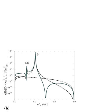
Figure 3: The differential branching ratios $dBr/dm^{2}_{ll}$ as a function of the invariant di-lepton mass $m_{ll}^{2}$ for the Cabibbo allowed decay $D_{s}^{+}\to\pi^{+}l^{+}l^{-}$ (a) and Cabibbo suppressed decay $D^{+}\to\pi^{+}l^{+}l^{-}$ (b). The dashed line denotes the long distance contribution, the dot-dashed line denotes the $c\to ul^{+}l^{-}$ induced short distance contribution, while the solid line denote the total standard model prediction. The $D_{s}^{+}\to\pi^{+}l^{+}l^{-}$ arises only via the long distance contribution.

The differential branching ratio $dBr/dm_{ll}^{2}$ for the Cabibbo allowed decay $D_{s}^{+}\to\pi^{+}l^{+}l^{-}$, which arises only via the weak annihilation, is presented in Fig. 3a. In Fig. 3b, we present the Cabibbo suppressed decay $D\to\pi l^{+}l^{-}$, in which the kinematical upper bound on di-lepton mass $m_{ll}^{max}=m_{D}-m_{P}$ is the highest. The dashed and dot-dashed lines denote the long and short distance parts of the rate in SM, respectively, while the solid lines denote the total rate. The long distance contribution decreases in the kinematical region above the resonance $\phi$ and the short distance contribution becomes dominant. Thus, the decays $D^{+,0}\to\pi^{+,0}l^{+}l^{-}$ at high $m_{ll}$ might present a unique opportunity to probe the flavour changing neutral transition $c\to ul^{+}l^{-}$ in the future. As the pion is the lightest hadron state, this interesting kinematical region is not present in other $D\to Xl^{+}l^{-}$ decays.

The differential distribution for $D^{+}\to\pi^{+}l^{+}l^{-}$, given in Fig. 3, indicates that the high di-lepton mass region might give an opportunity for detecting $c\to ul^{+}l^{-}$. Before making a definite statement on such possibility, we should examine this kinematical region of high di-lepton mass in $D\to\pi l^{+}l^{-}$ decays more closely. For instance, in this region the excited states of the vector mesons $\rho$, $\omega$ and $\phi$ may become important. We attempt a rough estimate of the additional long distance contribution arising from the first radial excited states $\rho_{1}$, $\omega_{1}$ and $\phi_{1}$ (${}^{3}S_{1}$) and first orbital excited states $\rho_{2}$, $\omega_{2}$ and $\phi_{2}$ (${}^{3}D_{1}$). The knowledge of their masses, decay widths and couplings to other particles is poor at present. We use the measured masses and widths, taken from [13, 35] and compiled in Table 5. Due to the lack of the experimental data on the leptonic decay widths [35], we use the magnitudes of the decay constants $g_{V}$ as predicted by the quark model in [36] and compiled in Table 5. At the same time, we assume that the excited vector mesons couple to the charmed mesons with the same couplings as the corresponding ground state vector mesons $\rho$, $\omega$ and $\phi$. In this case, the corresponding amplitudes (26) are obtained by replacing the coefficients $N_{1}$ and $M_{1}$ by the expressions given in (6). The differential branching ratios for $D\to\pi\mu^{+}\mu^{-}$ decays are given in Fig. 4. The thick and thin dashed lines denote the long distance contributions with and without excited vector mesons, respectively. The short distance contribution, denoted by dot-dashed line, is still dominant in the kinematical region of high $m_{ll}$ in spite of the excited vector resonances.

Figure 4: The differential branching ratio for $D\to\pi\mu^{+}\mu^{-}$ decays. The thick dashed lines present the long distance contribution incorporating the ground state and the excited vector mesons. The thin dashed lines present the long distance contributions due only to the ground vector mesons. The short distance contribution, denoted by dot-dashed line, is dominant in the kinematical region of high $m_{ll}$, in spite of the excited vector resonances.

Figure 5: The biggest possible enhancement of $D\to\pi\mu^{+}\mu^{-}$ rates within the general MSSM, discussed in section 2.1, is denoted by the dot-dashed lines. The solid lines represent the standard model predictions. The effect of supersymmetry is screened by the uncertainties present in the determination of the long distance contributions and is probably too small to be observed.

The possible enhancement within the general MSSM, discussed in section 2.1, is presented in Fig. 5 and is probably too small to be observed in any $D\to Pl^{+}l^{-}$ decay. The solid lines represent the standard model prediction for the $D\to\pi l^{+}l^{-}$ branching ratios. The dot-dashed lines represent the best enhancement in the general MSSM and indicate that the $D\to Pl^{+}l^{-}$ rates are rather insensitive to the large supersymmetric enhancement of $c_{7}$. The value of $c_{7}$ is manifested in $c\to ul^{+}l^{-}$ at small $m_{ll}$ (see Eq. (2) and Fig. 1), while it’s effect is suppressed in $D\to Pl^{+}l^{-}$ decays do to the factor $q^{2}$ in the general expression for the $D\to P\gamma^{*}$ amplitude (13).

5 Conclusions

We have presented the first predictions for rare charm meson decays $D\to Pl^{+}l^{-}$ with $P=\pi,K,\eta,\eta^{\prime}$ in all nine possible channels; the previous analysis [15] has considered only the $D\to\pi l^{+}l^{-}$ channel. The long distance contributions are found to dominate over the short distance contributions, which are induced by $c\to ul^{+}l^{-}$ in the Cabibbo-suppressed decays. We have used the theoretical framework of Heavy Meson Chiral Lagrangian with the recently determined value of the strong coupling $g$ from the measurement of $D^{*}\to D\pi$ width. Our predictions are compiled in Table 2. The decay $D^{+}_{s}\to\pi^{+}l^{+}l^{-}$ is predicted at the highest branching ratio of $6\times 10^{-6}$. The best chances of the experimental discovery are expected for $D^{+}\to\pi^{+}l^{+}l^{-}$, which is predicted at $1\times 10^{-6}$ and has the upper bound $8\times 10^{-6}$ [12] at present. The limits on $D^{0}$ and $D^{+}$ modes at the level $10^{-6}$ are expected from CLEO-c and B-factories, while the limits on $D_{s}^{+}$ modes are expected to be an order of magnitude milder [14].

The only possibility to look for $c\to ul^{+}l^{-}$ transition is represented by $D\to\pi l^{+}l^{-}$ decays in the kinematical region of $m_{ll}$ above the resonance $\phi$, where the long distance contribution is reduced (see Fig. 4).

We have explored the sensitivity of the $c\to ul^{+}l^{-}$ within two scenarios of physics beyond SM. The effect due the exchange of the flavour changing Higgs in Two Higgs Doublet model is found to be negligible. The general Minimal Supersymmetric Standard model can enhance the $c\to u\mu^{+}\mu^{-}$ rate by up to a factor of three (see Table 1). This effect is due to the large supersymmetric enhancement of $c_{7}$ and is seizable at small $m_{ll}$ in $c\to ul^{+}l^{-}$, but it is unfortunately very small in the hadronic process $D\to Pl^{+}l^{-}$ as the decay $D\to P\gamma$ is forbidden (see Fig. 5).

The kinematics of the processes $D\to Vl^{+}l^{-}$ would be more favorable to probe the possible supersymmetric enhancement at small $m_{ll}$, but the long distance contributions in these channels are even more disturbing [2]. The large supersymmetric enhancement of the Willson coefficient $c_{7}$ is manifested in $c\to u\gamma$ decay and can enhance the standard model rate $\sim 10^{-8}$ by up to two orders of magnitudes [6, 7]. Such enhancement could be probed by observation of $B_{c}\to B_{u}^{*}\gamma$ [3] or by measuring the relative difference $Br(D^{0}\to\rho^{0}\gamma)-Br(D^{0}\to\omega\gamma)$ [4].

6 Appendix

The short distance part of the $D\to Pl^{+}l^{-}$ amplitude, induced by the transition $c\to ul^{+}l^{-}$, contains the following form factors

$$\langle P(p^{\prime})|\bar{q}\gamma_{\mu}(1-\gamma_{5})c|D(p)\rangle =(p+p^{\prime})_{\mu}f_{+}(q^{2})+(p-p^{\prime})_{\mu}f_{-}(q^{2})$$

$$\langle P(p^{\prime})|\bar{q}\sigma_{\mu\nu}(1\pm\gamma_{5})c|D(p)\rangle =is(q^{2})\bigl{[}(p+p^{\prime})_{\mu}q_{\nu}-q_{\mu}(p+p^{\prime})_{\nu}\pm i\epsilon_{\mu\nu\lambda\sigma}(p+p^{\prime})^{\lambda}q^{\sigma}\bigr{]}$$ (22)

defined using operators in (1). The short distance amplitude is then given by

$${\cal A}^{SD}[D(p)\to P(p-q)l^{+}l^{-}]=i~{}\tfrac{G_{F}}{\sqrt{2}}e^{2}V_{cs}^{*}V_{us}\biggl{[}-\frac{c_{7}+c_{7}^{\prime}}{2\pi^{2}}m_{c}s(q^{2})-\frac{c_{9}}{4\pi^{2}}f_{+}(q^{2})\biggr{]}\bar{u}(p_{-})\!{\not\!p}v(p_{+})~{},$$ (23)

where we neglected the nearly vanishing $c_{10}$, $c_{9}^{\prime}$ and $c_{10}^{\prime}$ coefficients in SM (4) and MSSM (6). In the heavy quark limit, the form factor $s$ can be expressed in terms of the form factors $f_{\pm}$ at zero recoil [39] and we assume the relation to be valid for all $q^{2}$

$$s(q^{2})=\frac{1}{2m_{D}}\bigl{[}f_{+}(q^{2})-f_{-}(q^{2})\bigr{]}~{}.$$ (24)

The semileptonic form factors $f_{\pm}$ in the Heavy Meson Chiral Lagrangian approach, extended by assuming the polar shape, are given by [28, 29]

$$f_{+}(q^{2})=-f_{-}(q^{2})=-K_{DP}~{}\frac{f_{D}}{2}~{}\biggl{[}g\frac{m_{D}-m_{P}}{m_{P}+m_{D^{\prime*}}-m_{D}}\biggr{]}~{}\frac{m_{D^{\prime*}}^{2}-q^{2}_{max}}{m_{D^{\prime*}}^{2}-q^{2}}~{}.$$ (25)

with $K_{DP}$ given in Table 3.

The long distance amplitude is given by the diagrams in Fig. 2. The long distance penguin diagrams in Fig. 2a are expressed in terms of the form factor $f_{+}$ (25). The weak annihilation contribution in Fig. 2b is determined by assuming that the vertices do not change significantly away from the kinematical region, where the heavy quark and chiral symmetries are good. We expect this to be a reasonable approximation in $D$ meson decays. At the same time we use the full heavy meson propagators $1/(p_{D}^{2}-m^{2})$ instead of the HQET propagators $1/(2mvk)$ [31]. In the limit $m_{P}\ll m_{D}$, the bremsstrahlung-like diagrams in Fig. 2b cancel exactly, as explained in detail in the Sections 3.3.3 and 5.5.1 of [32]. Only the non-bremsstrahlung weak annihilation diagrams in Fig. 2a render the non-vanishing contribution. The long distance amplitude is given by [32]

$${\cal A}^{LD}[ D(p)\to P(p-q)l^{+}(p_{+})l^{-}(p_{-})]=i~{}\tfrac{G_{F}}{\sqrt{2}}~{}e^{2}~{}A^{LD}(q^{2})~{}\bar{u}(p_{-})\!{\not\!p}v(p_{+})~{},$$ (26)

$$A^{LD}(q^{2}) =A^{LD}_{peng.}(q^{2})+A^{LD}_{{annih.\atop bremsstrahlung}}(q^{2})+A^{LD}_{{annih.\atop non-brem.}}(q^{2})~{},$$

$$A^{LD}_{peng.}(q^{2}) =a_{2}V_{cs}^{*}V_{us}\frac{1}{q^{2}}f_{+}(q^{2})N_{1}(q^{2})~{},$$

$$A^{LD}_{annih.\atop bremsstrahlung}(q^{2}) \simeq 0~{},$$

$$A^{LD}_{annih.\atop non-brem.}(q^{2}) =f_{Cabb}^{(i)}\frac{1}{q^{2}}M_{1}^{(i)}(q^{2})f_{P}\biggl{[}-f_{D}\kappa\frac{m_{P}^{2}}{m_{D}^{2}-m_{P}^{2}}-\sqrt{m_{D}}\bigl{(}\alpha_{1}-\frac{m_{D}^{2}+m_{P}^{2}-q^{2}}{2m_{D}^{2}}\alpha_{2}\bigr{)}\biggr{]}\frac{\tilde{g}_{V}}{\sqrt{2}}~{}$$

with Cabibbo factors $f_{Cabb}^{(i)}$ and the coefficients $M_{1}(q^{2})$ and $K_{DP}^{(i)}$ as given in Table 3. The coefficient $N_{1}$ equals

$$N_{1}(q^{2}) ={g_{\rho}^{2}\over q^{2}-m_{\rho}^{2}+i\Gamma_{\rho}m_{\rho}}-{g_{\omega}^{2}\over 3(q^{2}-m_{\omega}^{2}+i\Gamma_{\omega}m_{\omega})}-{2g_{\phi}^{2}\over 3(q^{2}-m_{\phi}^{2}+i\Gamma_{\phi}m_{\phi})}$$

$$+{g_{\rho}^{2}\over m_{\rho}^{2}}-{g_{\omega}^{2}\over 3m_{\omega}^{2}}-{2g_{\phi}^{2}\over 3m_{\phi}^{2}}~{},$$

while the coefficients $M_{1}^{(i)}$ are given in terms of $M^{D^{0}}_{1}$, $M^{D^{+}}_{1}$ and $M^{D_{s}^{+}}$ in Table 3

$$M^{D^{0}}_{1}\!\!\! = \!\!\!{g_{\rho}\over q^{2}-m_{\rho}^{2}+i\Gamma_{\rho}m_{\rho}}+{g_{\omega}\over 3(q^{2}-m_{\omega}^{2}+i\Gamma_{\omega}m_{\omega})}+{g_{\rho}\over m_{\rho}^{2}}+{g_{\omega}\over 3m_{\omega}^{2}}~{},$$

$$M^{D^{+}}_{1}\!\!\! = \!\!\!-{g_{\rho}\over q^{2}-m_{\rho}^{2}+i\Gamma_{\rho}m_{\rho}}+{g_{\omega}\over 3(q^{2}-m_{\omega}^{2}+i\Gamma_{\omega}m_{\omega})}-{g_{\rho}\over m_{\rho}^{2}}+{g_{\omega}\over 3m_{\omega}^{2}}~{},$$

$$M^{D_{s}^{+}}_{1}\!\!\! = \!\!\!-{2g_{\phi}\over 3(q^{2}-m_{\phi}^{2}+i\Gamma_{\phi}m_{\phi})}-{2g_{\phi}\over 3m_{\phi}^{2}}~{}.$$ (27)

Note that $N_{1}(0)=M_{1}(0)=0$ for $\Gamma(0)=0$ and there is no pole arising from to the photon propagator at $q^{2}=0$. The relative sign of the short and long distance penguin amplitudes agrees with the Ref. [37], which is based on assumption of quark-hadron duality.

$i$	$D\to Pl^{+}l^{-}$	$f_{Cabb}^{(i)}$	$M^{(i)}$	$K_{DP}^{(i)}$
$1$	$D^{0}\to{\bar{K}}^{0}l^{+}l^{-}$	$a_{2}V_{ud}V_{cs}^{*}$	$M_{1}^{D^{0}}$	$0$
$2$	$D_{s}^{+}\to\pi^{+}l^{+}l^{-}$	$a_{1}V_{ud}V_{cs}^{*}$	$M_{1}^{D_{s}^{+}}$	$0$
$3$	$D^{0}\to\pi^{0}l^{+}l^{-}$	$-a_{2}V_{ud}V_{cd}^{*}$	$-\tfrac{1}{\sqrt{2}}M_{1}^{D^{0}}$	$\tfrac{1}{\sqrt{2}f_{\pi}}$
$4$	$D^{0}\to\eta l^{+}l^{-}$	$a_{2}V_{ud}V_{cd}^{*}$	$-\sqrt{\tfrac{3}{2}}M_{1}^{D^{0}}\cos\theta_{P}$	$\tfrac{\cos\theta_{P}}{\sqrt{6}f}-\tfrac{\sin\theta_{P}}{\sqrt{3}f}$
$5$	$D^{0}\to\eta^{\prime}l^{+}l^{-}$	$a_{2}V_{ud}V_{cd}^{*}$	$-\sqrt{\tfrac{3}{2}}M_{1}^{D^{0}}\sin\theta_{P}$	$\tfrac{\sin\theta_{P}}{\sqrt{6}f}+\tfrac{\cos\theta_{P}}{\sqrt{3}f}$
$6$	$D^{+}\to\pi^{+}l^{+}l^{-}$	$-a_{1}V_{ud}V_{cd}^{*}$	$M_{1}^{D^{+}}$	$\tfrac{1}{f_{\pi}}$
$7$	$D_{s}^{+}\to K^{+}l^{+}l^{-}$	$a_{1}V_{ud}V_{cd}^{*}$	$M_{1}^{D_{s}^{+}}$	$\tfrac{1}{f_{K}}$
$8$	$D^{+}\to K^{+}l^{+}l^{-}$	$-a_{1}V_{us}V_{cd}^{*}$	$M_{1}^{D^{+}}$	$0$
$9$	$D^{0}\to K^{0}l^{+}l^{-}$	$-a_{2}V_{us}V_{ud}^{*}$	$M_{1}^{D^{0}}$	$0$

Table 3: The Cabibbo factors $f_{Cabb}^{(i)}$, the coefficients $K_{DP}^{(i)}$ and the functions $M_{1}^{(i)}$ for nine $D\to Pl^{+}l^{-}$ amplitudes in (26).

$H$	$m_{H}$	$f_{H}$	$P$	$m_{P}$	$f_{P}$
	[GeV]	[GeV]		[GeV]	[GeV]
$D$	$1.87$	$0.21$	$\pi$	$0.14$	$0.135$
$D_{s}$	$1.97$	$0.24$	$K$	$0.50$	$0.16$
$D^{*}$	$2.01$	$0.21$	$\eta$	$0.55$	$0.13$
			$\eta^{\prime}$	$0.96$	$0.11$

Table 4: The values of the meson masses, decay constants and decay widths [13]. The measured decay constants $f_{D}$ and $f_{D^{*}}$ have sizable uncertainties and the values are taken from lattice QCD results [38].

	$\rho$	$\omega$	$\phi$	$\rho_{1}$	$\omega_{1}$	$\phi_{1}$	$\rho_{2}$	$\omega_{2}$	$\phi_{2}$
m[GeV]	0.77	0.78	1.0	1.45	1.46	1.69	1.66	1.66	1.88
$\Gamma$[GeV]	0.15	0.0084	0.0044	0.31	0.24	0.3	0.4	0.1	0.3
$g_{V}$[GeV2]	0.17	0.15	0.24	0.11	0.11	0.23	0.07	0.07	0.12

Table 5: The masses, widths and decay constants of ground [13] and excited [35, 36] vector mesons.

In order to account for the contributions of the excited vector mesons $\rho_{1,2}$, $\omega_{1,2}$ and $\phi_{1,2}$, as described in the main text, the coefficients $N_{1}$ and $M_{1}$ are replaced in the formulas above (26), (6) by

$$N_{1} \to N_{1}+\sum_{k=1}^{2}{g_{\rho_{k}}^{2}\over q^{2}-m_{\rho_{k}}^{2}+i\Gamma_{\rho_{k}}m_{\rho_{i}}}-{g_{\omega_{k}}^{2}\over 3(q^{2}-m_{\omega_{k}}^{2}+i\Gamma_{\omega_{k}}m_{\omega_{k}})}-{2g_{\phi_{k}}^{2}\over 3(q^{2}-m_{\phi_{k}}^{2}+i\Gamma_{\phi_{k}}m_{\phi_{k}})}$$

$$\qquad+{g_{\rho_{k}}^{2}\over m_{\rho_{k}}^{2}}-{g_{\omega_{k}}^{2}\over 3m_{\omega_{k}}^{2}}-{2g_{\phi_{k}}^{2}\over 3m_{\phi_{k}}^{2}}~{},$$

$$M^{D^{0}}_{1} \to M^{D^{0}}_{1}+\sum_{k=1}^{2}{g_{\rho_{k}}\over q^{2}-m_{\rho_{k}}^{2}+i\Gamma_{\rho_{k}}m_{\rho_{k}}}+{g_{\omega_{k}}\over 3(q^{2}-m_{\omega_{k}}^{2}+i\Gamma_{\omega_{k}}m_{\omega_{k}})}+{g_{\rho_{k}}\over m_{\rho_{k}}^{2}}+{g_{\omega_{k}}\over 3m_{\omega_{k}}^{2}}~{},$$

$$M^{D^{+}}_{1} \to M^{D^{+}}_{1}-\sum_{k=1}^{2}{g_{\rho_{k}}\over q^{2}-m_{\rho_{k}}^{2}+i\Gamma_{\rho_{k}}m_{\rho_{k}}}+{g_{\omega_{k}}\over 3(q^{2}-m_{\omega_{k}}^{2}+i\Gamma_{\omega_{k}}m_{\omega_{k}})}-{g_{\rho_{k}}\over m_{\rho_{k}}^{2}}+{g_{\omega_{k}}\over 3m_{\omega_{k}}^{2}}~{},$$

$$M^{D_{s}^{+}}_{1} \to M^{D_{s}^{+}}-\sum_{k=1}^{2}{2g_{\phi_{k}}\over 3(q^{2}-m_{\phi_{k}}^{2}+i\Gamma_{\phi_{k}}m_{\phi_{k}})}-{2g_{\phi_{k}}\over 3m_{\phi_{k}}^{2}}~{}.$$ (28)

References

- [1] G. Burdman, E. Golowich, J. Hewett and S. Pakvasa, Phys. Rev. D 52 (1995) 6383; A. Khodjamirian, G. Stoll and D. Wyler, Phys. Lett. B 358 (1995) 129; S. Fajfer, S. Prelovsek and P. Singer, Eur. Phys. J. C 6 (1999) 471, 751 (E).
- [2] S. Fajfer, S. Prelovsek and P. Singer, Phys. Rev. D 58 (1998) 094038.
- [3] S. Fajer, S. Prelovsek and P. Singer, Phys. Rev. D 59 (1999) 114003.
- [4] S. Fajfer, S. Prelovsek, P. Singer and D. Wyler, Phys. Lett B 487 (2000) 81.
- [5] B. Bajc, S. Fajfer, R. J. Oakes, Phys. Rev. D 54 (1996) 5883; P. Singer, Acta Phys. Pol. B 30 (1999) 3849, hep-ph/9911215.
- [6] S. Prelovsek and D. Wyler, Phys. Lett. B 500 (2001) 304.
- [7] I. Bigi, G. Gabbiani and A. Masiero, Z. Phys. C 48 (1990) 633.
- [8] The mixing predictions are compiled in H. Nelson, hep-exp/9908021.
- [9] R. Godang et al., CLEO Coll., Phys. Rev. Lett. 84 (2000) 5038; J.M. Link et al., FOCUS Coll., Phys. Lett. B 485 (2000) 62.
- [10] E.M. Aitala et al., E791 Coll., Phys. Rev. Lett. 86 (2001) 3969; D. Sanders, hep-ex/0009027; D. J. Summers, hep-ph/0011079, hep-ex/0010002; A. J. Schwartz, hep-ex/0101050.
- [11] E. M. Aitala et al., E791 Coll., Phys. Lett. B 462 (1999) 401; D. A. Sanders, hep-ex/0105028.
- [12] H. Park, hep-ex/0005044, talk “D mixing and rare decays” at International conference on B physics and CP Violation, Taipei, Taiwan (1999), http://www.phys.ntu.edu.tw/english/bcp3/; D. Pedrini, talk at Kaon99, http://sgimida/mi/infn/it/-pedrini/conf-talks.html.
- [13] Review of Particle Physics, D.E. Groom et al., Eur. J. C 15 (2000) 1.
- [14] M. Selen, Workshop on Prospects for CLEO/CESR with , Cornell University, May 5-7, 2001, http://www.lns.cornell.edu/public/CLEO/CLEO-C/; M. Selen, private communication.
- [15] P. Singer and D.-X. Zhang, Phys. Rev. D 55 (1997) R1127.
- [16] E. Lunghi, A. Masiero, I. Scimemi and L. Silvestrini, Nucl. Phys. B 568 (2000) 120.
- [17] T. Inami and C. S. Lim, Prog. Theor. Phys. 65 (1981) 297; A. J. Schwartz, Mod. Phys. Lett. A 8 (1993) 967.
- [18] C. Greub, T. Hurth, M. Misiak and D. Wyler, Phys. Lett. B 382 (1996) 415.
- [19] G. Buchalla, A. Buras, M.E. Leutenbacher, Rev. Mod. Phys. 68 (1996) 1125.
- [20] M.J. Duncan, Nucl. Phys. B 211 (1983) 285; J. F. Donoghue, H.P. Nilles and D. Wyler, Phys. Lett. B 128 (1983) 55.
- [21] M. Misiak, S. Pokorski and J. Roseik, Heavy Flavours II, ed. A. Buras and M. Lindner, World Scentific 1998, p. 795 (hep-ph/9703442).
- [22] J.A. Casas and S. Dimopoulos, Phys. Lett. B 387 (1996) 107.
- [23] F. Gabbiani, E. Gabrielli, A. Masiero and L. Silvestrini, Nucl. Phys. B 477 (1996) 321.
- [24] T. P. Cheng, M. Sher, Phys. Rev. D 15 (1987) 2484, M. Sher, Y. Yuan, Phys. Rev. D 44 (1991) 1461.
- [25] G. Castro, R. Martinez and J. Munoz, Phys. Rev. D 58 (1998) 033003.
- [26] G. Ecker, A. Pich and E. Rafael, Nucl. Phys. B 291 (1987) 692.
- [27] M. Bauer, B. Stech and M. Wirbel, Z. Phys. C 34 (1987) 103; M. Neubert , V. Rieckert, B. Stech and Q. P. Xu, in: Heavy Flavours, eds. A. J. Buras and M. Linder (World Scientific, Singapore, 1992) p. 286.
- [28] M. Wise, Phys. Rev. D 45 (1992) R2188; G. Burdman and J. F. Donoghue, Phys. Lett. B 280 (1992) 287.
- [29] R. Casalbuoni et al., Phys. Rept. 281 (1997) 145.
- [30] M. Bando et al., Phys. Rev. Lett 54 (1985) 1215; Nucl. Phys. B259 (1985) 493; Phys. Rep. 164 (1988) 217.
- [31] B. Bajc, S. Fajfer and R. J. Oakes, Phys, Rev. D 53 (1996) 4957.
- [32] S. Prelovsek, Ph. D. thesis, hep-ph/0010106.
- [33] CLEO Coll., T. E. Coan et al., hep-ex/0102007; M. Dubrovin (for CLEO Coll.) hep-ex/0105030.
- [34] S. Fajfer, P. Singer, Phys. Rev. D 56 (1997) 4302.
- [35] A.B. Clegg and A. Donnachie, Z. Phys. C 62 (1994) 455.
- [36] S. Godfrey and N. Isgur, Phys. Rev. D 32 (1985) 189.
- [37] N. Paver, Riazuddin, Phys. Rev. D 45 (1992) 978.
- [38] C. Bernard et al., MILC Coll., hep-lat/9909121; A. Abada et al., hep-lat/9910021.
- [39] N. Isgur, M.B. Wise, Phys. Rev. D 42 (1990) 2388.