Resumming the color-octet contribution to radiative $\Upsilon$ decay

Abstract

At the upper endpoint of the photon energy spectrum in $\Upsilon\to X\gamma$, the standard NRQCD power counting breaks down and the OPE gives rise to color-octet structure functions. Furthermore, in this kinematic regime large Sudakov logarithms appear in the octet Wilson coefficients. The endpoint spectrum can be treated consistently within the framework of a recently developed effective field theory of collinear and soft particles. Here we show that within this approach the octet structure functions arise naturally and that Sudakov logarithms can be summed using the renormalization group equations. We derive an expression for the resummed energy spectrum and, using a model lightcone structure function, investigate the phenomenological importance of the resummation.

I Introduction

Early theoretical analyses of heavy quarkonium decay were based on the color-singlet model (CSM). The underlying assumption of this model is that the heavy-quark–antiquark pair has the same quantum numbers as the quarkonium meson. (For example the $b\bar{b}$ that forms an $\Upsilon$ must be in a color-singlet ${}^{3}S_{1}$ configuration.) One consequence of such a restrictive assumption is that theoretical predictions based on the CSM are simple, depending on only one nonperturbative parameter. The quantities first calculated in the CSM were the inclusive rates for quarkonium to decay into leptons and into light hadrons [1]. Subsequently the direct photon spectrum in inclusive radiative quarkonium decays was calculated [2].

In recent years the simple CSM has been superseded by a nonrelativistic effective theory of QCD (NRQCD) [3, 4]. Inclusive decays of quarkonium are now understood in the framework of the operator product expansion (OPE), supplemented by the power-counting rules of NRQCD. In this formalism the direct photon spectrum of $\Upsilon$ decay is

$$\frac{d\Gamma}{dz}=\sum_{i}C_{i}(M,z)\langle\Upsilon|{\cal O}_{i}|\Upsilon\rangle\,,$$ (1)

where $z=2E_{\gamma}/M$, with $M=2m_{b}$. The $C_{i}$ are short-distance Wilson coefficients which can be calculated as a perturbative series in $\alpha_{s}(M)$, and the ${\cal O}_{i}$ are NRQCD operators. NRQCD power-counting rules assign a power of the relative velocity $v$ of the heavy quarks to each operator and organizes the series. The series may be truncated at any order with omitted terms suppressed by powers of $v$. For $S$-wave mesons the formally leading-order contribution is the color-singlet operator, which is related to the wavefunction at the origin. Thus for $S$-wave decays one recovers the CSM at leading order in $v$. At higher orders in $v$ color-octet operators need to be included.

However, the picture of the photon spectrum in $\Upsilon\to X\gamma$ decay which emerges is much richer than the naive expectation that the color-singlet contribution is leading [5, 6, 7]. At low values of the photon energy, fragmentation contributions to $\Gamma(\Upsilon\to X\gamma)$ are important [8, 5]. The situation at large values of the photon energy is even more interesting, because both the OPE and perturbative expansion break down. The breakdown of the OPE was first addressed in Ref. [7]. It was shown that the color-octet contributions, which give rise to a singular contribution at maximum photon energy, become leading for large photon energies. The singular nature is smeared by a nonperturbative structure function, which tames the endpoint behavior of the photon spectrum. The breakdown of the perturbative expansion gives rise to so-called Sudakov logarithms which have to be resummed. In a recent work [9] it was pointed out that the leading Sudakov logarithms cancel in the CSM. However this is not the case for Sudakov logarithms in the color-octet contribution.

Both the breakdown of the OPE and the appearance of Sudakov logarithms are symptoms of the same disease: NRQCD does not contain the correct low energy degrees of freedom to describe the endpoint of the photon spectrum. It does not contain collinear quarks and gluons. A theory constructed from the appropriate degrees of freedom was developed in Refs. [10, 11]. In those papers the theory was applied to the decay of a single heavy quark to light degrees of freedom. It was shown that the renormalization group equations (RGEs) in this theory sums Sudakov logarithms. In addition, for inclusive decays at the endpoint, the nonperturbative structure function arises naturally from a modified version of the OPE. Here we apply the theory to the color-octet contributions to radiative $\Upsilon$ decay. In Section II we discuss the leading contributions in the endpoint region and motivate perturbative and nonperturbative resummation. In Section III we sum Sudakov logarithms using the RGEs in an effective field theory. In Section IV we introduce a phenomenological model for the shape function, convolute it with the resummed spectrum, and show how this changes the color-octet contribution to the spectrum. In Section V we conclude.

II Leading order results

The inclusive radiative differential decay rate of $\Upsilon$ can be calculated using the optical theorem. This relates the decay rate to the imaginary part of the forward matrix element of the time ordered product of two currents

$$\frac{d\Gamma}{dz}=\frac{M^{2}}{8\pi^{2}}\,z\,\langle\Upsilon|{\rm Im}\,T|\Upsilon\rangle\,,$$ (2)

where we have used nonrelativistic normalization for the states: $\langle\Upsilon(P^{\prime})|\Upsilon(P)\rangle=(2\pi)^{3}\delta^{3}(P^{\prime}-P)$. For large momentum transfer the time ordered product can be expanded in terms of local operators giving

$$\frac{d\Gamma}{dz}=\sum_{i}C_{i}(z)\langle\Upsilon|{\cal O}_{i}|\Upsilon\rangle\,.$$ (3)

The Wilson coefficients, $C_{i}(z)$, can be calculated perturbatively as a series in $\alpha_{s}(M)$. The parametric size of the long distance matrix elements are determined by power counting in NRQCD, but to obtain quantitative results these matrix elements have to be extracted from experiments or lattice calculations.

At leading order in the NRQCD $v$ expansion, only the color-singlet, spin-triplet operator

$${\cal O}_{\bf 1}(^{3}S_{1})=\sum_{{\bf p},{\bf p}^{\prime}}[\psi^{\dagger}_{{\bf p}^{\prime}}\sigma^{i}\chi_{-{\bf p}^{\prime}}]\;[\chi^{\dagger}_{-{\bf p}}\sigma^{i}\psi_{{\bf p}}]$$ (4)

contributes, with the leading order Wilson coefficient

$$C_{\bf 1}^{(0)}(^{3}S_{1})(z) = \frac{128\,\alpha_{s}^{2}\,\alpha\,e_{Q}^{2}}{27M^{2}}\,\Theta(1-z)$$ (6)

$$\times\left[\frac{2-z}{z}+\frac{z(1-z)}{(2-z)^{2}}+2\frac{1-z}{z^{2}}\log(1-z)-2\frac{(1-z)^{2}}{(2-z)^{3}}\log(1-z)\right]\,,$$

where $e_{Q}=-1/3$ for $\Upsilon$. This is the CSM result [2], with $\langle\Upsilon|{\cal O}_{\bf 1}({}^{3}S_{1})|\Upsilon\rangle\approx(3/2\pi)|R(0)|^{2}$, where $R(0)$ is the radial wavefunction at the origin. The first color-octet contributions to (3) are suppressed by $v^{4}$ relative to this color-singlet contribution. There are two operators

$${\cal O}_{\bf 8}(^{1}S_{0}) = \sum_{{\bf p},{\bf p}^{\prime}}[\psi^{\dagger}_{{\bf p}^{\prime}}\,T^{a}\,\chi_{-{\bf p}^{\prime}}]\;[\chi^{\dagger}_{-{\bf p}}\,T^{a}\,\psi_{{\bf p}}]\,,$$ (7)

$${\cal O}_{\bf 8}(^{3}P_{0}) = \frac{1}{3}\sum_{{\bf p},{\bf p}^{\prime}}[\psi^{\dagger}_{{\bf p}^{\prime}}\,{\bf p}^{\prime}\cdot\mbox{\boldmath$\sigma$}\,T^{a}\chi_{-{\bf p}^{\prime}}]\;[\chi^{\dagger}_{-{\bf p}}\,{\bf p}\cdot\mbox{\boldmath$\sigma$}\,T^{a}\psi_{{\bf p}}]\,,$$ (8)

with leading order Wilson coefficients[5]

$$C_{i}^{(0)}(z)=\tilde{C}_{i}^{(0)}\delta(1-z)\,,$$ (9)

where

$$\tilde{C}_{\bf 8}^{(0)}(^{1}S_{0}) = \frac{16\,\alpha_{s}\,\alpha\,e_{Q}^{2}\pi}{M^{2}},$$ (10)

$$\tilde{C}_{\bf 8}^{(0)}(^{3}P_{0}) = \frac{448\,\alpha_{s}\,\alpha\,e_{Q}^{2}\pi}{M^{4}}\,.$$ (11)

Since the color-octet Wilson coefficients are enhanced by a power of $\alpha_{s}(M)/\pi$ relative to the color-singlet one, the overall suppression of the color-octet contribution is $\pi v^{4}/\alpha_{s}(M)\sim v^{2}$, where we have used that numerically $\alpha_{s}/\pi\sim v^{2}$.

The singular nature of the coefficients (9) is an indication that the OPE is breaking down. We can obtain a rough estimate for the value of $z$ at which the octet contributions become of order the color-singlet contribution by smearing the perturbative spectrum over a small region near $z=1$. Integrating over $1-v^{2}<z<1$ gives a color-singlet contribution that scales as $\alpha^{2}_{s}(M)v^{2}$ and a color-octet contribution that scales as $\alpha_{s}(M)\pi v^{4}$. Thus, the ratio of octet to singlet in this region of phase space is $\pi v^{2}/\alpha_{s}(M)\sim 1$, making the color-octet contribution of the same order as the color-singlet one.

It was shown in Ref. [7] that in precisely this endpoint region the OPE breaks down and an infinite set of operators have to be resummed into lightcone distribution functions $f_{i}(k_{+})$. Each structure function gives the probability to find a $b\bar{b}$ pair with the appropriate quantum numbers and residual momentum $k_{+}$ in the $\Upsilon$. For the color-singlet contribution the structure function can be calculated using the vacuum saturation approximation. It simply shifts the maximal photon energy from $2m_{b}$ to $M_{\Upsilon}$ [7]. The color-octet contributions, however, give rise to two new nonperturbative functions at leading order. At higher order there are an infinite number of additional structure functions, so the differential decay rate in the endpoint region is

$$\frac{d\Gamma}{dz}=\sum_{i}\int dk_{+}C_{i}(z,k_{+})f_{i}(k_{+})\langle\Upsilon|{\cal O}_{i}|\Upsilon\rangle\,.$$ (12)

Another effect one encounters in the endpoint region is the appearance of Sudakov logarithms in the Wilson coefficients, which ruin the perturbative expansion. Consider, for example, the Wilson coefficients for the color-octet operators at next-to-leading order in $\alpha_{s}$. In the $z\to 1$ limit they are [5]

$$C_{\bf 8}^{(1)}(^{1}S_{0})(z) = \frac{\alpha_{s}}{2\pi}\tilde{C}_{\bf 8}^{(0)}(^{1}S_{0})\left[-2C_{A}\left(\frac{\log(1-z)}{1-z}\right)_{+}-\left(\frac{23}{6}C_{A}-\frac{n_{f}}{3}\right)\left(\frac{1}{1-z}\right)_{+}\right],$$ (13)

$$C_{\bf 8}^{(1)}(^{3}P_{0})(z) = \frac{\alpha_{s}}{2\pi}\tilde{C}_{\bf 8}^{(0)}(^{3}P_{0})\left[-2C_{A}\left(\frac{\log(1-z)}{1-z}\right)_{+}-\left(\frac{23}{6}C_{A}-\frac{n_{f}}{3}\right)\left(\frac{1}{1-z}\right)_{+}\right].$$ (14)

If these coefficients are integrated over the shape-function region ($1-v^{2}<z<1$), then the first plus distribution on the right-hand side gives rise to a double logarithm, $\log^{2}v^{2}$, while the second plus distribution gives a single logarithm, $\log v^{2}$. Both of these are numerically of order $1/\alpha_{s}$. This clearly ruins the perturbative expansion. Therefore, to obtain a well controlled expansion, these logarithms must be summed.

III Summing Sudakov Logarithms

The NRQCD power-counting rules break down as $z\to 1$ because NRQCD does not include all of the long distance modes: collinear physics is missing from the theory. An effective theory which includes collinear physics was developed in Refs. [10, 11]. This collinear-soft theory describes the interactions of highly energetic collinear modes with soft degrees of freedom. To describe $\Upsilon$ decay at the endpoint we have to couple the collinear-soft theory with NRQCD [4]. This is analogous to $B\to X_{s}\gamma$ decays at the endpoint, which was studied in the context of effective field theory in Ref. [10]. We will closely follow the development in that paper.

Understanding inclusive $\Upsilon\to X\gamma$ decays near the endpoint is a two-step process. In the first step we must integrate out the large scale, $M=2m_{b}$, set by the $b\bar{b}$ pair constituting the $\Upsilon$. This is done by matching onto the collinear-soft theory. In the second step collinear modes are integrated out at a scale which is set by the invariant mass of the collinear jet. This is done by performing an OPE and matching onto a soft theory containing operators which are nonlocal along the lightcone and whose matrix elements are the lightcone distribution functions, $f_{i}(k_{+})$. Sudakov logarithms are summed by using the effective theory RGEs. Operators are run from the hard scale $M$ to the collinear scale where the OPE is performed. The nonlocal soft operators are then run from the collinear scale down to a soft scale where their matrix elements do not contain large logarithms. This procedure sums all Sudakov logarithms into the short distance coefficient functions.

To better understand the scales involved consider the momentum of a collinear particle moving near the lightcone. In lightcone coordinates we can write this momentum as $p=(p^{+},p^{-},p_{\perp})$. Since the mass of the particle is much smaller than its energy, we define $p^{2}\sim M^{2}\lambda^{2}$, where $M$ is the scale that sets the energy and $\lambda$ is a small parameter. The lightcone momentum components are widely separated. If we choose $p^{-}$ to be ${\cal O}(M)$, then $p_{\perp}/p^{-}\sim\lambda$, and $p^{+}/p^{-}\sim\lambda^{2}$. We refer to these two scales as collinear and soft, respectively. To be concrete consider the $b\bar{b}$ pair to have momentum $Mv^{\mu}+k^{\mu}$, where $v^{\mu}=(1,0,0,0)$ and $k^{\mu}$ is ${\cal O}(\Lambda_{\rm QCD})$ in the $\Upsilon$ center-of-mass frame. The photon momentum is $Mz\bar{n}^{\mu}/2$, where we have chosen $\bar{n}^{\mu}=(1,0,0,1)$. In the endpoint region the hadronic jet recoiling against the photon moves in the opposite lightcone direction $n^{\mu}=(1,0,0,-1)$, with momentum $p^{\mu}_{X}=Mn^{\mu}/2+M(1-z)\bar{n}^{\mu}/2+k^{\mu}$ . Thus the hadronic jet has $\bar{n}\cdot p_{X}=p^{-}_{X}\sim M$. Next note that $m^{2}_{X}\approx M^{2}(1-z)$. For $(1-z)\sim v^{2}\sim\Lambda_{\rm QCD}/M$ we find

$$m_{X}\sim\sqrt{M\Lambda_{\rm QCD}}\,,$$ (15)

which is the collinear scale. This implies that for this process the collinear-soft expansion parameter $\lambda$ is of order $\sqrt{1-z}\sim\sqrt{\Lambda_{\rm QCD}/M}$. The soft scale is the component of the hadronic momentum in the $n$ direction:

$$n\cdot p_{X}\sim\frac{m^{2}_{X}}{\bar{n}\cdot p_{X}}\sim\Lambda_{\rm QCD}\sim M\lambda^{2}\,.$$ (16)

Thus in order to sum Sudakov logarithms in $\Upsilon\to X\gamma$ we first match onto the collinear-soft theory at $M$ and run operators in this theory down to the collinear scale $\mu_{c}\sim M\sqrt{1-z}$. At that scale we perform the OPE by matching onto a soft theory containing operators that are nonlocal along the lightcone and run these operators down to the soft scale $\mu_{s}\sim M(1-z)$.

A The collinear-soft theory

We first need to integrate out the large scale $M$ by matching onto the collinear-soft theory. This is done by calculating matrix elements in QCD, expanding them in powers of $\lambda$, and matching onto products of Wilson coefficients and operators in the effective theory. For the process of interest this matching is illustrated in Fig. 1.

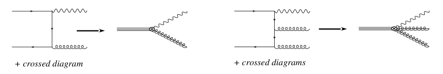
FIG. 1.: Matching onto operators in the effective field theory with one and two gluons in the final state.

The heavy-quark spinors and the heavy-quark propagator in QCD can be expanded in powers of $v$ to match onto NRQCD. The QCD spinor is decomposed into two two-component Pauli spinors $\psi$ and $\chi$ for the heavy quark and anti-quark, respectively [14]. We also need to expand the amplitude in powers of $\lambda$ to match onto the collinear-soft theory. This is done by using the power-counting rules for the gluon field given in Ref. [11] and by scaling the different components of the gluon momentum as

$$p_{g}^{\mu} = p_{g}\cdot\bar{n}\,\frac{n^{\mu}}{2}+p_{g\perp}^{\mu}+p_{g}\cdot n\,\frac{\bar{n}^{\mu}}{2}$$ (17)

$$= {\cal O}(1)+{\cal O}(\lambda)+{\cal O}(\lambda^{2})\,.$$ (18)

Omitting the straightforward but unenlightening details, the color-octet contributions match in the $\Upsilon$ rest frame, at leading order in $\lambda$, onto the operators

$$Q_{\bf 8}^{\mu}(^{1}S_{0}) = 2ig_{s}e_{b}\,\epsilon^{\alpha\mu}_{\perp}\;\sum_{\bf p}[\chi^{\dagger}_{-{\bf p}}T^{a}\psi_{\bf p}]\,A^{a}_{\alpha}\,,$$ (19)

$$Q_{\bf 8}^{\mu}(^{3}P_{J}) = 4g_{s}e_{b}\left(g_{\perp}^{\alpha\delta}g^{\mu\sigma}+g_{\perp}^{\alpha\sigma}g^{\mu\delta}-g_{\perp}^{\alpha\mu}\bar{n}^{\sigma}\bar{n}^{\delta}\right)\;\sum_{\bf p}\Lambda\cdot\widehat{\bf p}_{\sigma}[\chi^{\dagger}_{-{\bf p}}\Lambda\cdot\sigma_{\delta}T^{a}\psi_{\bf p}]\,A^{a}_{\alpha}\,,$$ (20)

where $\epsilon^{\alpha\mu}_{\perp}=\epsilon^{\alpha\mu\rho\beta}\bar{n}_{\rho}v_{\beta}$ and $g_{\perp}^{\mu\nu}=g^{\mu\nu}-(n^{\mu}\bar{n}^{\nu}+n^{\nu}\bar{n}^{\mu})/2$. Hatted variables are divided by $M$, and the $\Lambda^{\mu i}$ are boost matrices which boost from the $b\bar{b}$ center-of-mass frame [14]. We have chosen factors in the operators such that at leading order the corresponding Wilson coefficients satisfy

$$C_{\bf 8}^{Q}({}^{1}S_{0})=C_{\bf 8}^{Q}({}^{3}P_{0})\equiv C_{\bf 8}^{Q}=1\,.$$ (21)

Note that there is no color-singlet operator at this order in $\lambda$, and therefore leading Sudakov logarithms are absent in the CSM [9].

To calculate the renormalization group equations of these operators, we also need the Feynman rules shown in Table I. They are all obtained by expanding full theory diagrams in powers of $\lambda$ and $v$. In addition the coupling of soft gluons is given by HQET and LEET [15] Feynman rules, and the coupling of three collinear gluons is identical to the three gluon vertex in QCD.

TABLE I.: Feynman rules in the collinear-soft theory at leading order in $\lambda$. The vertices $V_{{\bf 1},{\bf 8}}(^{3}S_{1})$, $V_{{\bf 1},{\bf 8}}(^{1}P_{1})$ have a zero matching coefficient at this order.

$\displaystyle\begin{array}[]{ll}\hbox{Diagram}&\hbox{Feynman Rule}\\ \hline\cr\hline\cr&\\ \lower 55.0pt\hbox{\epsfbox{softcolcol.ps}}&\frac{1}{2}g_{s}f^{abc}n^{\mu}(2g^{\nu\rho}\bar{n}\cdot p-\bar{n}^{\nu}p^{\rho}-\bar{n}^{\rho}p^{\nu}-\bar{n}^{\nu}\bar{n}^{\rho}\bar{n}\cdot k)\\ &\\ \lower 35.0pt\hbox{\epsfbox{vertexleading.ps}}&\begin{array}[]{l}V^{\alpha\mu a}_{\bf 8}({}^{1}S_{0})=-2g_{s}e_{b}\epsilon^{\alpha\mu}_{\perp}\;\eta^{\dagger}_{-{\bf p}}T^{a}\xi_{\bf p}\\ \\ V^{\alpha\mu a}_{\bf 8}({}^{3}P_{0})=4ig_{s}e_{b}(g^{\alpha\delta}_{\perp}g^{\mu\sigma}+g^{\alpha\sigma}_{\perp}g^{\mu\delta}-g^{\alpha\mu}_{\perp}\bar{n}^{\mu}\bar{n}^{\delta})\\ \qquad\qquad\qquad\qquad\qquad\times\Lambda\cdot\widehat{{\bf p}}_{\sigma}\eta^{\dagger}_{-{\bf p}}\Lambda\cdot\mbox{\boldmath$\sigma$}_{\delta}T^{a}\xi_{\bf p}\end{array}\\ &\\ \lower 30.0pt\hbox{\epsfbox{vertexsub.ps}}&\begin{array}[]{l}\tilde{V}^{\alpha\beta ab}_{\bf 8}(^{1}S_{0})=\frac{i}{2}g_{s}^{2}e_{b}f^{abc}\,\left(\epsilon^{\beta\mu}_{\perp}\frac{\bar{n}^{\alpha}}{\bar{n}\cdot p_{1}}-\epsilon^{\alpha\mu}_{\perp}\frac{\bar{n}^{\beta}}{\bar{n}\cdot p_{2}}\right)\;\eta^{\dagger}_{-{\bf p}}T^{c}\xi_{\bf p}\\ \\ \tilde{V}^{\alpha\beta ab}_{\bf 8}(^{3}P_{J})=-g_{s}^{2}e_{b}\ f^{abc}\ \left[\frac{\bar{n}^{\beta}}{\bar{n}\cdot p_{2}}\left(g_{\perp}^{\alpha\delta}g^{\mu\sigma}+g_{\perp}^{\alpha\sigma}g^{\mu\delta}-g_{\perp}^{\alpha\mu}n^{\sigma}n^{\delta}\right)\right.\\ \qquad\qquad\qquad\qquad\left.\,-\,\frac{\bar{n}^{\alpha}}{\bar{n}\cdot p_{1}}\left(g_{\perp}^{\beta\delta}g^{\mu\sigma}+g_{\perp}^{\beta\sigma}g^{\mu\delta}-g_{\perp}^{\beta\mu}n^{\sigma}n^{\delta}\right)\right]\\ \qquad\qquad\qquad\qquad\qquad\qquad\times\Lambda\cdot\widehat{\bf p}_{\sigma}\;\eta^{\dagger}_{-{\bf p}}\Lambda\cdot\mbox{\boldmath$\sigma$}_{\delta}T^{c}\xi_{\bf p}\end{array}\end{array}$

The renormalization is independent of the operator and the two diagrams that need to be calculated are shown in Fig. 2.

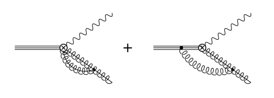
FIG. 2.: Collinear and soft diagrams needed to calculate the renormalization of the vertices in the effective theory.

The result for the collinear and soft graphs are

$${\cal A}_{c} = \frac{\alpha_{s}C_{A}}{4\pi}\left(4\pi\frac{\mu^{2}}{(-1-i\delta)p_{g}^{2}}\right)^{\epsilon}\frac{\Gamma^{2}(1-\epsilon)\Gamma(1+\epsilon)}{\Gamma(2-2\epsilon)}\frac{2-3\epsilon}{\epsilon^{2}}\,V_{i}^{\alpha\mu a}\,,$$ (22)

$${\cal A}_{s} = -\frac{\alpha_{s}C_{A}}{4\pi}\left(4\pi\frac{\mu^{2}(\bar{n}\cdot p_{g})^{2}}{(-1-i\delta)^{2}p_{g}^{4}}\right)^{\epsilon}\Gamma(1+\epsilon)\Gamma(1+2\epsilon)\Gamma(1-2\epsilon)\frac{1}{\epsilon^{2}}\,V_{i}^{\alpha\mu a}\,,$$ (23)

where $V_{i}^{\alpha\mu a}=(V^{\alpha\mu a}_{\bf 8}(^{1}S_{0}),V^{\alpha\mu a}_{\bf 8}(^{3}P_{J}))$.

To renormalize the vertex, we expand in $\epsilon$, keeping only the divergent pieces. This must equal $(Z-1)V^{\alpha\mu a}_{i}$. Note however that $Z$ is not the counterterm for the vertex, rather $Z_{\cal O}=Z_{h\bar{h}}Z^{1/2}_{3}Z^{-1}Z_{\gamma}^{1/2}$, where $Z_{\gamma}=1$ since we are not considering QED corrections, $Z_{h\bar{h}}$ is the counterterm of the color-octet $h_{v}\bar{h}_{v}$ current, and $Z_{3}$ is the gluon wave function counterterm:

$$Z_{h\bar{h}} = 1+\frac{\alpha_{s}C_{A}}{4\pi}\frac{1}{\epsilon}\,,$$ (24)

$$Z_{3} = 1+\frac{\alpha_{s}}{4\pi}\frac{1}{\epsilon}\left(C_{A}\frac{5}{3}-n_{f}\frac{2}{3}\right)\,.$$ (25)

This leads to

$$Z_{\cal O}-1=\frac{\alpha_{s}}{4\pi}\left[C_{A}\left(\frac{1}{\epsilon^{2}}+\frac{1}{\epsilon}\log\left(\frac{\mu^{2}}{M^{2}}\right)+\frac{17}{6\epsilon}\right)-\frac{n_{f}}{3\epsilon}\right]\,.$$ (26)

We can check this result by matching the effective theory to QCD while regulating all divergences using dimensional regularization. In this approach there is no scale in effective theory loop integrals so they are zero. This leaves only the counterterm $Z$, which must match the $\epsilon$ poles in the QCD calculation. The QCD vertex at one loop can be extracted from a calculation by Maltoni, Mangano, and Petrelli [16]. Equating the pole terms in the QCD calculation to $Z$ we again obtain (26).

The RGE for the Wilson coefficients of the operators in (19) is

$$\mu\frac{d}{d\mu}C_{i}^{Q}(\mu)=\gamma^{Q}(\mu)C_{i}^{Q}(\mu)\,.$$ (27)

In order to make use of previous results from $B\to X_{s}\gamma$, we write the anomalous dimension in the same form as in Ref. [17]

$$\gamma^{Q}(\mu)=-\Gamma_{\rm cusp}^{\rm adj}\log\frac{\mu}{m_{b}}+\frac{B+2\gamma}{2}\,.$$ (28)

Defining

$$\Gamma_{\rm cusp}^{\rm adj} = \frac{\alpha_{s}(\mu)}{\pi}\Gamma^{\rm adj}_{1}+\left(\frac{\alpha_{s}(\mu)}{\pi}\right)^{2}\Gamma^{\rm adj}_{2}\,,\quad B=\frac{\alpha_{s}(\mu)}{\pi}B_{1}\,,\quad\gamma=\frac{\alpha_{s}(\mu)}{\pi}\gamma_{1},$$ (29)

we find

$$\Gamma^{\rm adj}_{1}=C_{A},\quad B_{1}+2\gamma_{1}=-C_{A}-\frac{\beta_{0}}{2}\,,$$ (30)

where $\beta_{0}=(11C_{A}-2n_{f})/3$. At this point we can only determine the above linear combination of $B_{1}$ and $\gamma_{1}$, and we do not know the expression for $\Gamma^{\rm adj}_{2}$. However, as we will show below, $B_{1}$ and $\Gamma^{\rm adj}_{2}$ can be found in the soft theory. To sum the leading Sudakov logarithms in the collinear-soft theory, we run the operator given in (19) from the matching scale $\mu=M$ down to a scale $\mu_{c}\sim\sqrt{M\Lambda_{\rm QCD}}$ at which the OPE is performed. We can lift the solution from Ref. [11]

$$\log\bigg{[}\frac{C_{V}(\mu)}{C_{V}(M)}\bigg{]} = -\frac{4\pi\Gamma^{\rm adj}_{1}}{\beta_{0}^{2}\>\alpha_{s}(M)}\>\Big{[}\frac{1}{y}-1+\log y\Big{]}-\frac{\Gamma^{\rm adj}_{1}\beta_{1}}{\beta_{0}^{3}}\Big{[}1-y+y\log y-\frac{1}{2}\log^{2}y\Big{]}$$ (32)

$$-\frac{B_{1}+2\gamma_{1}}{\beta_{0}}\log y-\frac{4\Gamma^{\rm adj}_{2}}{\beta_{0}^{2}}\Big{[}y-1-\log y\Big{]}\,,$$

where $y=\alpha_{s}(\mu)/\alpha_{s}(M)$.

B The purely Soft Theory

At the collinear scale $\mu_{c}\approx M\sqrt{1-z}$ we integrate out collinear modes and perform an OPE for the inclusive $\Upsilon$ radiative decay rate in the endpoint region. The result is a nonlocal OPE in which the two currents are separated along a light-like direction. Diagrammatically this is illustrated in Fig. 3. We write the momentum of the jet as

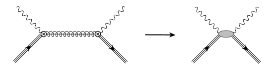
FIG. 3.: The leading OPE: tree level matching of the time ordered product in the collinear-soft theory to a nonlocal operator in the soft theory.

$$p_{X}=\frac{M}{2}n^{\mu}+k^{\mu}+\frac{M}{2}(1-x)\bar{n}^{\mu}\,,$$ (33)

where $k^{\mu}$ is the residual momentum of the $b\bar{b}$ pair. Note we distinguish $x$ from $z$, because the momentum of the jet is not exactly the same as the momentum of the collinear gluon which was integrated out. The two can differ slightly due to the emission of soft quanta by the jet. The imaginary part of the tree level diagram on the left hand side of Fig. 3 is proportional to $\delta(p^{2}_{x})$. Taking $k^{\mu}\sim M(1-x)\sim M\lambda^{2}$ and expanding in the small parameter $\lambda$, we match at leading order onto the operator

$${\cal O}_{i}(x)=\sum_{{\bf pp}^{\prime}}[\psi^{\dagger}_{{\bf p}^{\prime}}\Gamma_{i}^{\prime}\chi_{-{\bf p}^{\prime}}]\,\delta(1-x+i\hat{D}^{+})\,[\chi^{\dagger}_{-{\bf p}}\Gamma_{i}\psi_{{\bf p}}]\,,$$ (34)

where $\Gamma_{\bf 8}(^{1}S_{0})=T^{a}$ and $\Gamma_{\bf 8}(^{3}P_{0})=T^{a}\,{\bf p}\!\cdot\!\mbox{\boldmath$\sigma$}/\sqrt{3}$. The $x$ serves as a continuous label on the operator.

Each operator has a Wilson coefficient, which can depend on the photon energy fraction $z$. The differential decay rate is given by a convolution of the matrix elements of the operators ${\cal O}_{i}(x)$ and the corresponding Wilson coefficients

$$\frac{d\Gamma}{dz}=\sum_{i}\int\!dx\,C_{i}(x-z;\mu)f_{i}(x;\mu)\langle\Upsilon|{\cal O}_{i}|\Upsilon\rangle\,,$$ (35)

where

$$f_{i}(x,\mu)=\frac{\langle\Upsilon|{\cal O}_{i}(x;\mu)|\Upsilon\rangle}{\langle\Upsilon|{\cal O}_{i}|\Upsilon\rangle}$$ (36)

are the lightcone distribution functions.

The convolution of the short distance Wilson coefficients and the long distance operators presents a technical problem since the RGE for ${\cal O}(x)$ will be given in terms of a convolution as well. We use a Mellin transform to deconvolute (35), which is equivalent to taking moments of the decay rate. We must restrict ourselves to large moments $N$, since it is the limit $N\to\infty$ which is equivalent to the region $z\to 1$. Once the the final expression in moment space is obtained we can take an inverse-Mellin transform to get back to $z$-space. This procedure is valid up to corrections of order $1-z$. Taking large moments of the expression in (35) gives

$$\Gamma(N)\equiv\int dz\,z^{N-1}\frac{d\Gamma}{dz}=\sum_{i}C_{i}(N;\mu)f_{i}(N;\mu)\,,$$ (37)

where

$$f_{i}(N;\mu)\equiv\int x^{N-1}f_{i}(x;\mu)\,.$$ (38)

To match onto the soft theory, we compare large moments of the differential decay rate calculated in the collinear-soft effective theory and the soft effective theory in the parton model. Large moments of the one loop expression calculated in the collinear-soft theory are given in (A12). The one loop expression for $\langle b\bar{b}|{\cal O}(N;\mu)|b\bar{b}\rangle$ can be lifted from Ref. [10] with the replacement $C_{F}\to C_{A}$:

$$\langle b\bar{b}|{\cal O}(N;\mu)|b\bar{b}\rangle=1-\frac{\alpha_{s}C_{A}}{4\pi}\left[4\log^{2}\frac{\mu N}{Mn_{0}}-4\log\frac{\mu N}{Mn_{0}}\right]\,,$$ (39)

where $n_{0}=e^{-\gamma_{E}}$. At the scale $\mu_{c}=M\sqrt{n_{0}/N}$ all logarithms match, and at that scale the tree level matching coefficients are

$$C_{i}(N;\mu)=\tilde{C}^{(0)}_{i}\left[C^{Q}(M\sqrt{n_{0}/N})\right]^{2}\,.$$ (40)

In the matrix element (39) all logarithms vanish at the scale $\mu_{s}=Mn_{0}/N$. To sum the large logarithms, we therefore have to run the Wilson coefficient in the soft theory, $C_{i}(N;\mu)$, from $\mu_{c}=M\sqrt{n_{0}/N}$ to $\mu_{s}=Mn_{0}/N$. Again, we keep the notation introduced for $B\to X_{s}\gamma$ and write the RGE as

$$\mu\frac{d}{d\mu}C_{i}(N;\mu)=\gamma(N;\mu)C_{i}(N;\mu),$$ (41)

with

$$\gamma(N;\mu)=2\Gamma_{\rm cusp}^{\rm adj}(\mu)\log\frac{\mu N}{Mn_{0}}+B\,.$$ (42)

From the results in Refs. [10, 18, 19] and the previous section we obtain

$$\Gamma^{\rm adj}_{1} = C_{A},\quad\Gamma^{\rm adj}_{2}=C_{A}\left[C_{A}\left(\frac{67}{36}-\frac{\pi^{2}}{12}\right)-\frac{5n_{f}}{18}\right],$$ (43)

$$B_{1} = -C_{A}\,,\quad\gamma_{1}=-\frac{\beta_{0}}{4}\,,$$ (44)

where we have taken $\Gamma^{\rm adj}_{2}$ from Refs. [18, 19].

The solution to (41) combined with the running in the collinear-soft theory (32) can be lifted directly from Ref. [17] by substituting into that result the expressions in (43). This gives the fully resummed result in moment space

$$\Gamma(N)=\sum_{i}\tilde{C}^{(0)}_{i}f(N;Mn_{0}/N)e^{\log(N)g_{1}(\chi)+g_{2}(\chi)},$$ (45)

where

$$g_{1}(\chi) = -\frac{2\Gamma^{\rm adj}_{1}}{\beta_{0}\chi}\left[(1-2\chi)\log(1-2\chi)-2(1-\chi)\log(1-\chi)\right],$$ (46)

$$g_{2}(\chi) = -\frac{8\Gamma^{\rm adj}_{2}}{\beta_{0}^{2}}\left[-\log(1-2\chi)+2\log(1-\chi)\right]$$ (49)

$$-\frac{2\Gamma^{\rm adj}_{1}\beta_{1}}{\beta_{0}^{3}}\left[\log(1-2\chi)-2\log(1-\chi)+\frac{1}{2}\log^{2}(1-2\chi)-\log^{2}(1-\chi)\right]$$

$$+\frac{4\gamma_{1}}{\beta_{0}}\log(1-\chi)+\frac{2B_{1}}{\beta_{0}}\log(1-2\chi)-\frac{4\Gamma^{\rm adj}_{1}}{\beta_{0}}\log n_{0}\left[\log(1-2\chi)-\log(1-\chi)\right]\,,$$

$\chi=\log(N)\,\alpha_{s}(M)\beta_{0}/4\pi$, and $\beta_{1}=(34C_{A}^{2}-10C_{A}n_{f}-6C_{F}n_{f})/3$.

IV Results

Now that we have the resummed rate in moment space (45), we must take the inverse-Mellin transform to obtain the expression for the photon energy spectrum. Fortunately, the inverse-Mellin transform of the resummed rate in $B\to X_{s}\gamma$ decay has been calculated in Ref. [20], and we can use that result by simply substituting in the $g_{i}$ from (46). We obtain the following for the resummed Wilson coefficients of the octet contribution

$$C_{i}(x-z)=-\,\tilde{C}_{i}^{(0)}\,\frac{d}{dz}\left\{\theta(x-z)\;\frac{\exp[lg_{1}[\alpha_{s}\beta_{0}l/(4\pi)]+g_{2}[\alpha_{s}\beta_{0}l/(4\pi)]]}{\Gamma[1-g_{1}[\alpha_{s}\beta_{0}l/(4\pi)]-\alpha_{s}\beta_{0}l/(4\pi)g_{1}^{\prime}[\alpha_{s}\beta_{0}l/(4\pi)]]}\right\}\,,$$ (50)

where $\tilde{C}^{(0)}_{i}=\tilde{C}^{(0)}_{\bf 8}(^{1}S_{0})$, $\tilde{C}^{(0)}_{\bf 8}(^{3}P_{0})$, and $l\approx-\log(x-z)$. Each $C_{i}(x-z)$ is evaluated at the soft scale so that all leading and next-to-leading Sudakov logarithms have been summed into it.

One way of checking (50) is by expanding in powers of $\alpha_{s}$ and comparing to the fixed order calculation. Using

$$\left(\frac{\log^{n}(1-z)}{1-z}\right)_{+}=\lim_{\eta\to 0}\left[\theta(1-z-\eta)\frac{\log^{n}(1-z)}{1-z}+\delta(1-z)\,\frac{\log^{n+1}(\eta)}{n+1}\right],$$ (51)

as the definition for plus distributions it is straightforward to verify that the order $\alpha_{s}$ term in the expansion of (50) reproduces the plus distributions in (13).

Recall that the covariant derivative in (34) is of order $\Lambda_{\rm QCD}/M$. If we consider the limit $1-z\gg\Lambda_{\rm QCD}/M$, then the covariant derivative in the operator appearing in the structure function can be neglected. In this limit we can perform the integral in (35) to obtain

$$\frac{d\Gamma}{dz}=\sum_{i}C_{i}(1-z)\,.$$ (52)

This result gives the effect of the perturbative resummation without the structure function. The quantity $C_{i}(1-z)/\tilde{C}^{(0)}_{i}$, which is the same for the two leading octet configurations, is shown as the dashed line in Fig. 4.

However, for the $b\bar{b}$ system $mv^{2}\sim\Lambda_{\rm QCD}$ so the covariant derivative cannot be dropped in the endpoint region of the photon spectrum, and the differential rate is given by the convolution in (35). The lightcone distribution function is a nonperturbative function and needs to be modelled. In this paper we will be content with the simple structure functions introduced in Ref. [22] for inclusive $B$ decays

$$f(k^{+}) = N\left(1-\frac{k^{+}}{\bar{\Lambda}}\right)^{a}\,e^{(1+a)k^{+}/\bar{\Lambda}}\;,$$ (53)

where $N$ is chosen so that the integral of the structure function is normalized to one. In principle the structure function can be different for the different color-octet states. But since we are ignorant of the nonperturbative structure function, we will naively use the same model for both the ${}^{1}S_{0}$ and ${}^{3}P_{0}$ configurations. The structure function for $B$ mesons have the property that the first moment with respect to $k^{+}$ vanishes. For quarkonium the first moment of (36) (where $x=1+\hat{k}^{+}$) with respect to $\hat{k}^{+}$ is

$$\Lambda_{1}=\frac{\langle\Upsilon|\sum_{{\bf p},{\bf p^{\prime}}}[\chi^{\dagger}_{-{\bf p^{\prime}}}T^{a}\Gamma_{i}\psi_{\bf p^{\prime}}]i\hat{D}^{+}[\psi^{\dagger}_{{\bf p}}T^{a}\Gamma_{i}\chi_{-{\bf p}}]|\Upsilon\rangle}{\langle\Upsilon|\sum_{{\bf p},{\bf p^{\prime}}}[\chi^{\dagger}_{-{\bf p^{\prime}}}T^{a}\Gamma_{i}\psi_{\bf p^{\prime}}][\psi^{\dagger}_{\bf p}T^{a}\Gamma_{i}\chi_{-\bf p}]|\Upsilon\rangle}\,.$$ (54)

Therefore, we need to shift $k^{+}$ in (53) to $k^{+}+\Lambda_{1}$, so that (53) will have the desired first moment for quarkonium decays. The integration limits for $k^{+}$ are, similar to the case for $B$ decays, from $-M$ to $M_{\Upsilon}-M$. Both $\bar{\Lambda}$ and $\Lambda_{1}$ are nonperturbative parameters related through $\bar{\Lambda}=M_{\Upsilon}-M-\Lambda_{1}$. We use the following numbers in our plots: $\alpha_{s}=0.2$, $\alpha=1/137$, $m_{b}=4.8\,{\rm GeV}$, $M_{\Upsilon}=9.46\,{\rm GeV}$, $a=1$, $\bar{\Lambda}=480\,{\rm MeV}$, and $\Lambda_{1}=-620\,{\rm MeV}$.

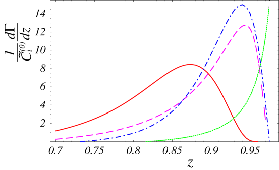
FIG. 4.: The differential decay spectra near the endpoint region $0.7<z$ in arbitrary units. The solid curve is the perturbative resummation convoluted with the structure function and the dashed curve is the perturbative resummation $C_{i}(1-z)/\tilde{C}^{(0)}_{i}$. The dotted curve is the plus distribution terms in the one-loop result (13), and the dot-dashed curve is these terms convoluted with the structure function.

In Fig. 4 the convolution of $C_{i}(x-z)/\tilde{C}^{(0)}_{i}$ with the model of the structure function (53) is shown as the solid line. In addition we show as the dotted line the terms in the NLO QCD expression that dominate in the endpoint region (13) divided by $\tilde{C}^{(0)}_{i}$, and as the dot-dashed line the convolution of these terms with (53). Thus Fig. 4 gives a picture of the effects of resummation. The singular plus distribution piece of the NLO QCD expression is tamed by both the perturbative resummation and the structure function. Either of these alone gives a similar curve, which is peaked near $z=0.94$. However, to be consistent the perturbative resummation must be convoluted with the structure function. This gives a curve that is broader, with a peak that is $34\%$ lower and shifted to $z=0.87$. Changing the values of the structure function parameters changes the shape of the curve. Halving the value of $\bar{\Lambda}$ gives a narrower peak that is $30\%$ lower and shifted to $z=0.83$. If $\alpha_{s}$ is increased by $10\%$ the peak moves slightly to the left and decreases in height by $5\%$. Doubling the value of $a$ in (53) slightly raises the peak, and steepens the curve as it goes to zero at the endpoint.

In Fig. 5, we show as dashed curves the fully resummed color-octet contribution convoluted with the structure function for two choices of the matrix elements. We also show as the solid curve the color-singlet contribution. Here we used

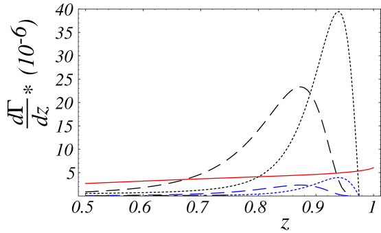
FIG. 5.: The differential decay spectra in the region $0.5<z$. The dashed curves are the fully resummed result convoluted with the shape function for two choices of the octet matrix elements. In addition we have interpolated the fully resummed result with the NLO result in the region away from the endpoint. The dotted curves are the NLO result convoluted with the structure function for two choices of the matrix elements. The solid curve is the color-singlet contribution.

$\langle\Upsilon|{\cal O}_{\bf 1}(^{3}S_{1})|\Upsilon\rangle=3.63\ {\rm GeV}^{3}$ [23]. The values of the color-octet matrix elements are not well determined. One may be tempted to use a naive power-counting argument which gives $\langle\Upsilon|{\cal O}_{\bf 8}(^{1}S_{0})|\Upsilon\rangle\sim\langle\Upsilon|{\cal O}_{\bf 8}(^{3}P_{0})|\Upsilon\rangle/m_{b}^{2}\sim v^{4}\langle\Upsilon|{\cal O}_{\bf 1}(^{3}S_{1})|\Upsilon\rangle$, with $v^{2}\sim 0.1$. However, this gives values for the color-octet matrix elements that are too large to be compatible with data on the ratio of hadronic to leptonic decays [5]. The data suggest that the octet matrix elements are at least an order of magnitude smaller than the naive power-counting estimate. Therefore, we use values that are 10 times and 100 times smaller than estimates from naive power counting, with the larger matrix element yielding the higher peak. We have added to the resummed result the NLO QCD result with the singular terms (13) subtracted off. This interpolates between the NLO QCD expression at lower values of $z$ and the resummed result in the endpoint region. For comparison we show as the dotted curves the NLO QCD contribution [5] convoluted with the shape function for the two choices of the color-octet matrix elements.

Since the octet contributions dominate the color-singlet contribution in this endpoint region (or at least are of the same order of magnitude) it should be possible to use this process to constrain the size of the color octet matrix element. The suppression of the matrix element compared to the naive power counting estimate makes a measurement of this matrix element particularly interesting and might shed some light on the convergence of the $v$ expansion in NRQCD. However, before a meaningful comparison of theory to data on radiative $\Upsilon$ decay can be made, subleading Sudakov logarithms in the color-singlet contribution must be summed. The existence of these logarithms was first pointed out in Ref. [9] where it was observed that though leading Sudakov logarithms cancel in the color-singlet contribution to the differential rate, they are present in the derivative of the rate at the endpoint. We leave the resummation of these logarithms to a future publication [25].

V conclusion

Using an effective field theory approach, we have resummed Sudakov logarithms in the leading color-octet contributions to the $\Upsilon\to X\gamma$ differential decay rate in the endpoint region. This is done in two steps. First we match onto an effective theory with collinear and soft degrees of freedom and run the theory to the collinear scale. Next we integrate out collinear modes by performing an OPE, matching onto non-local operators which are run to the soft scale. This sums all Sudakov logarithms into Wilson coefficients of these operators. The color-octet contribution to the differential decay rate in the endpoint region is given by the convolution of the Wilson coefficients with matrix elements of the operators between $\Upsilon$ states. The latter are the color-octet structure functions defined in Ref. [7].

We choose a simple model for the structure functions to investigate the phenomenological consequences of resummation. We find that either the perturbative resummation or the inclusion of a structure function cures the singular behavior of the QCD results. Both give a similar effect, causing the curve to turn over near $z=0.94$ and to go to zero at the endpoint. However, the effective field theory approach makes it clear that the correct expression for the differential rate near the endpoint is given by a convolution of the perturbative resummation and the structure function. This gives a spectrum that has a broader and lower peak than we obtain by including only perturbative resummation or the structure function, shifting the peak to $z=0.87$.

Before a meaningful comparison to data can be made the color-singlet result must be resummed as well. Only then can data on the decay spectrum be used to constrain the size of the octet contribution in the endpoint region [25].

A Forward scattering matrix element

Matching the forward scattering matrix element in the QCD and collinear-soft theory gives an important check that we are reproducing the infrared physics of the full theory. We have already calculated the vertex corrections. Note that there are two contributions from the vertex loops so the vertex contribution to the forward scattering matrix element is twice that given in (22). There is a contribution to the forward scattering matrix element from a ladder graph, which we have not evaluated yet. It gives

$${\cal M}_{\ell}=\frac{\alpha_{s}C_{A}}{2\pi}\left(4\pi\frac{\mu^{2}(\bar{n}\cdot p_{g})^{2}}{(-1-i\delta)^{2}p_{g}^{4}}\right)^{\epsilon}\Gamma(1+\epsilon)\Gamma(1+2\epsilon)\Gamma(1-2\epsilon)\frac{1}{\epsilon}\,{\cal M}_{0}\,,$$ (A1)

where

$${\cal M}_{0}=\tilde{C}^{(0)}_{i}\frac{M^{2}}{p^{2}_{g}-i\delta}$$ (A2)

is the tree level amplitude, and $p^{2}_{g}=M^{2}(1-z)$. In addition there is a contribution coming from virtual corrections to the collinear gluon propagator, which include the fermion, gluon, and ghost loops,

$${\cal M}_{Z_{3}}=\frac{\alpha_{s}}{4\pi}\left(\frac{5}{3}C_{A}-\frac{2}{3}n_{f}\right)\left(\frac{\mu^{2}}{(-1-i\delta)p_{g}^{2}}\right)^{\epsilon}\frac{1}{\epsilon}\,{\cal M}_{0}\,.$$ (A3)

Adding all contributions gives the full one-loop corrections to the forward scattering amplitude

$${\cal M}_{\rm lg} = \frac{\alpha_{s}}{2\pi}\left\{C_{A}\left[\frac{1}{\epsilon^{2}}+\frac{1}{\epsilon}\log\left(\frac{\mu^{2}}{M^{2}}\right)+\frac{17}{6\epsilon}\right]-\frac{n_{f}}{3\epsilon}+\frac{C_{A}}{2}\log^{2}\left(\frac{\mu^{2}}{M^{2}}\right)+\frac{17C_{A}}{6}\log\left(\frac{\mu^{2}}{M^{2}}\right)\right.$$ (A6)

$$\qquad-\left.\frac{n_{f}}{3}\log\left(\frac{\mu^{2}}{M^{2}}\right)-C_{A}\log^{2}[(1-z)(-1-i\delta)]-C_{A}\frac{23}{6}\log[(1-z)(-1-i\delta)]\right.$$

$$\qquad+\left.\frac{n_{f}}{3}\log[(1-z)(-1-i\delta)]\right\}{\cal M}_{0}+\dots\,,$$

where the ellipses represent terms of order $\alpha_{s}$ not enhanced by logarithms.

Next add the counterterms. There is a gluon propagator insertion that gives $-{\cal M}_{0}(Z_{3}-1)$. The vertex insertion is $Z_{h\bar{h}}Z^{1/2}_{3}Z^{-1}_{O}$. In order to facilitate the comparison with the results in Ref. [5], we use dimensional regularization to regulate the infrared divergences in the heavy quark sector, and therefore $Z_{h\bar{h}}=1$. Adding all the counterterms cancels the $\epsilon$ poles in (A6), leaving

$${\cal M}_{\rm lg} = \frac{\alpha_{s}}{2\pi}\left\{C_{A}\left[\frac{1}{2}\log^{2}\left(\frac{\mu^{2}}{M^{2}}\right)+\frac{17}{6}\log\left(\frac{\mu^{2}}{M^{2}}\right)\right]-\frac{n_{f}}{3}\log\left(\frac{\mu^{2}}{M^{2}}\right)-C_{A}\log^{2}[(1-z)(-1-i\delta)]\right.$$ (A8)

$$\qquad-\left.C_{A}\frac{23}{6}\log[(1-z)(-1-i\delta)]+\frac{n_{f}}{3}\log[(1-z)(-1-i\delta)]\right\}{\cal M}_{0}+\dots\,.$$

To obtain the differential decay rate we take $-1/\pi\;{\rm Im}$(A8) using

$$\frac{-1}{\pi}{\rm Im}\frac{\log[(1-z)(-1-i\delta)]}{1-z+i\delta} = \left(\frac{1}{1-z}\right)_{+}\,,$$ (A9)

$$\frac{-1}{\pi}{\rm Im}\frac{\log^{2}[(1-z)(-1-i\delta)]}{1-z+i\delta} = 2\left(\frac{\log(1-z)}{1-z}\right)_{+}-\pi^{2}\delta(1-z)\,.$$ (A10)

Comparing to Ref. [5] (taking the limit $z\to 1$ in their expressions), we confirm that at the matching scale $\mu=M$ the effective theory reproduces the plus distributions in the full theory. Taking large moments of the imaginary part of (A8) gives:

$$-\frac{1}{\pi}\int dz\;z^{N-1}\;{\rm Im}{\cal M}_{\rm lg} = \frac{\alpha_{s}}{2\pi}\left\{C_{A}\left[\frac{1}{2}\log^{2}\left(\frac{\mu^{2}}{M^{2}}\right)+\frac{17}{6}\log\left(\frac{\mu^{2}}{M^{2}}\right)\right]-\frac{n_{f}}{3}\log\left(\frac{\mu^{2}}{M^{2}}\right)\right.$$ (A12)

$$\qquad\left.-C_{A}\log^{2}\left[\frac{N}{n_{0}}\right]+C_{A}\frac{23}{6}\log\left[\frac{N}{n_{0}}\right]-\frac{n_{f}}{3}\log\left[\frac{N}{n_{0}}\right]\right\}\tilde{C}^{(0)}_{i}+\dots\,.$$

REFERENCES

- [1] T. Appelquist and H. D. Politzer, Phys. Rev. Lett. 34, 43 (1975).
- [2] S. J. Brodsky, D. G. Coyne, T. A. DeGrand and R. R. Horgan, Phys. Lett. B 73, 203 (1978); K. Koller and T. Walsh, Nucl. Phys. B 140, 449 (1978).
- [3] G. T. Bodwin, E. Braaten and G. P. Lepage, Phys. Rev. D 51, 1125 (1995) [Erratum-ibid. D 55, 5853 (1995)] [hep-ph/9407339].
- [4] M. E. Luke, A. V. Manohar and I. Z. Rothstein, Phys. Rev. D 61, 074025 (2000) [hep-ph/9910209].
- [5] F. Maltoni and A. Petrelli, Phys. Rev. D 59, 074006 (1999) [hep-ph/9806455].
- [6] S. Wolf, Phys. Rev. D 63, 074020 (2001) [hep-ph/0010217].
- [7] I. Z. Rothstein and M. B. Wise, Phys. Lett. B 402, 346 (1997) [hep-ph/9701404].
- [8] S. Catani and F. Hautmann, Nucl. Phys. Proc. Suppl. 39BC, 359 (1995) [hep-ph/9410394].
- [9] F. Hautmann, hep-ph/0102336.
- [10] C. W. Bauer, S. Fleming and M. Luke, Phys. Rev. D 63, 014006 (2001) [hep-ph/0005275].
- [11] C. W. Bauer, S. Fleming, D. Pirjol and I. W. Stewart, Phys. Rev. D 63, 114020 (2001) [hep-ph/0011336].
- [12] M. Neubert, Phys. Rev. D 49, 3392 (1994) [hep-ph/9311325]; M. Neubert, Phys. Rev. D 49, 4623 (1994) [hep-ph/9312311].
- [13] A. V. Manohar, J. Soto and I. W. Stewart, Phys. Lett. B 486, 400 (2000) [hep-ph/0006096].
- [14] E. Braaten and Y.Q. Chen, Phys. Rev. D54, 3216 (1996).
- [15] M. J. Dugan and B. Grinstein, Phys. Lett. B 255, 583 (1991).
- [16] F. Maltoni, M. L. Mangano, and A. Petrelli, Nucl. Phys. B519, 361 (1998).
- [17] R. Akhoury and I. Z. Rothstein, Phys. Rev. D 54, 2349 (1996) [hep-ph/9512303].
- [18] G. P. Korchemsky and A. V. Radyushkin, Sov. J. Nucl. Phys. 45, 127 (1987) [Yad. Fiz. 45, 198 (1987)].
- [19] G. P. Korchemsky and G. Marchesini, Nucl. Phys. B 406, 225 (1993) [hep-ph/9210281].
- [20] A. K. Leibovich, I. Low and I. Z. Rothstein, Phys. Rev. D 61, 053006 (2000) [hep-ph/9909404].
- [21] A. K. Leibovich, I. Low and I. Z. Rothstein, hep-ph/0105066.
- [22] A. L. Kagan and M. Neubert, Eur. Phys. J. C 7, 5 (1999) [hep-ph/9805303]; F. De Fazio and M. Neubert, JHEP 9906, 017 (1999) [hep-ph/9905351].
- [23] E. Braaten, S. Fleming and A. K. Leibovich, Phys. Rev. D 63, 094006 (2001) [hep-ph/0008091].
- [24] A. Petrelli, M. Cacciari, M. Greco, F. Maltoni and M. L. Mangano, Nucl. Phys. B 514, 245 (1998) [hep-ph/9707223].
- [25] C. W. Bauer, C. W. Chiang, S. Fleming, A. K. Leibovich, and I. Low, work in progress.