*Authors
J.A. Aguilar–Saavedra39, J. Alcaraz59, A. Ali26, S. Ambrosanio19, A. Andreazza68, J. Andruszkow48, B. Badelek111,113, A. Ballestrero110, T. Barklow102, A. Bartl114, M. Battaglia19,43, T. Behnke26, G. Belanger2, D. Benson76, M. Berggren84, W. Bernreuther1, M. Besançon98, J. Biebel26, O. Biebel73, I. Bigi76, J.J. van der Bij36, T. Binoth2, G.A. Blair56, C. Blöchinger115, J. Blümlein26, M. Boonekamp98, E. Boos71, G. Borissov80, A. Brandenburg26, J.–C. Brient83, G. Bruni15,16, K. Büsser26, P. Burrows82, R. Casalbuoni34, C. Castanier6, P. Chankowski113, A. Chekanov4, R. Chierici19, S.Y. Choi21, P. Christova27,100, P. Ciafaloni52, D. Comelli32, G. Conteras64, M. Danilov70, W. Da Silva84, A. Deandrea19, W. de Boer46, S. De Curtis34, S.J. De Jong74, A. Denner90, A. De Roeck19, K. Desch40, E. De Wolf3, S. Dittmaier26, V. Djordjadze26, A. Djouadi69, D. Dominici34, M. Doncheski88, M.T. Dova50, V. Drollinger46, H. Eberl114, J. Erler89, A. Eskreys48, J.R. Espinosa61, N. Evanson63, E. Fernandez8, J. Forshaw63, H. Fraas115, A. Freitas26, F. Gangemi86, P. Garcia-Abia19,10, R. Gatto37, P. Gay6, T. Gehrmann19, A. Gehrmann–De Ridder46, U. Gensch26, N. Ghodbane26, I.F. Ginzburg77, R. Godbole7, S. Godfrey81, G. Gounaris106, M. Grazzini116, E. Gross93, B. Grzadkowski113, J. Guasch46, J.F. Gunion25, K. Hagiwara47, T. Han46, K. Harder26, R. Harlander14, R. Hawkings26, S. Heinemeyer14, R.–D. Heuer40, C.A. Heusch99, J. Hewett102,103, G. Hiller102, A. Hoang73, W. Hollik46, J.I. Illana26,39, V.A. Ilyin71, D. Indumathi20, S. Ishihara44, M. Jack26, S. Jadach48, F. Jegerlehner26, M. Jeżabek48, G. Jikia36, L. Jönsson57, P. Jankowski, P. Jurkiewicz48, A. Juste8,31, A. Kagan22, J. Kalinowski113, M. Kalmykov26, P. Kalyniak81, B. Kamal81, J. Kamoshita78, S. Kanemura65, F. Kapusta84, S. Katsanevas58, R. Keranen46, V. Khoze28, A. Kiiskinen42, W. Kilian46, M. Klasen40, J.L. Kneur69, B.A. Kniehl40, M. Kobel17, K. Kołodziej101, M. Krämer29, S. Kraml114, M. Krawczyk113, J.H. Kühn46, J. Kwiecinski48, P. Laurelli35, A. Leike72, J. Letts45, W. Lohmann26, S. Lola19, P. Lutz98, P. Mättig93, W. Majerotto114, T. Mannel46, M. Martinez8, H.–U. Martyn1, T. Mayer115, B. Mele96,97, M. Melles90, W. Menges40, G. Merino8, N. Meyer40, D.J. Miller55, D.J. Miller26, P. Minkowski12, R. Miquel9,8, K. Mönig26, G. Montagna86,87, G. Moortgat–Pick26, P. Mora de Freitas83, G. Moreau98, M. Moretti32,33, S. Moretti91, L. Motyka111,49, G. Moultaka69, M. Mühlleitner69, U. Nauenberg23, R. Nisius19, H. Nowak26, T. Ohl24, R. Orava42, J. Orloff6, P. Osland11, G. Pancheri35, A.A. Pankov38, C. Papadopoulos5, N. Paver108,109, D. Peralta9,8, H.T. Phillips56, F. Picinini86,87, W. Placzek49, M. Pohl37,74, W. Porod112, A. Pukhov71, A. Raspereza26, D. Reid75, F. Richard80, S. Riemann26, T. Riemann26, S. Rosati17, M. Roth54, S. Roth1, C. Royon98, R. Rückl115, E. Ruiz–Morales60, M. Sachwitz26, J. Schieck41, H.–J. Schreiber26, D. Schulte19, M. Schumacher26, R.D. Settles73, M. Seymour63, R. Shanidze105,30, T. Sjöstrand57, M. Skrzypek48, S. Söldner–Rembold36, A. Sopczak46, H. Spiesberger62, M. Spira90, H. Steiner51, M. Stratmann92, Y. Sumino107, S. Tapprogge19, V. Telnov18, T. Teubner1, A. Tonazzo66, C. Troncon67, O. Veretin26, C. Verzegnassi109, A. Vest1, A. Vicini46, H. Videau83, W. Vogelsang94, A. Vogt53, H. Vogt26, D. Wackeroth95, A. Wagner26, S. Wallon84,79, G. Weiglein19, S. Weinzierl85, T. Wengler19, N. Wermes17, A. Werthenbach26, G. Wilson63, M. Winter104, A.F. Żarnecki113, P.M. Zerwas26, B. Ziaja48,111, J. Zochowski13.
\addsec
*Convenors A. Bartl, M. Battaglia, W. Bernreuther, G. Blair, A. Brandenburg, P. Burrows, K. Desch, A. Djouadi, W. de Boer, A. De Roeck, G. Gounaris, E. Gross, C.A. Heusch, S. Jadach, F. Jegerlehner, S. Katsanevas, M. Krämer, B.A. Kniehl, J. Kühn, W. Majerotto, M. Martinez, H.-U. Martyn, R. Miquel, K. Mönig, T. Ohl, M. Pohl, R. Rückl, M. Spira, V. Telnov, G. Wilson
1
RWTH Aachen, Germany
2
Laboratoire d’Annecy–le–Vieux de Physique des Particules, France
3
Universiteit Antwerpen, The Netherlands
4
ANL, Argonne, IL, USA
5
Demokritos National Centre for Scientific Research, Athens, Greece
6
Université Blaise Pascal, Aubière, France
7
Indian Institute of Science, Bangalore, India
8
Universitat Autonoma de Barcelona, Spain
9
Universitat de Barcelona, Spain
10
Universität Basel, Switzerland
11
University of Bergen, Norway
12
Universität Bern, Switzerland
13
Bialystok University Bialystok, Poland
14
BNL, Upton, NY, USA
15
INFN, Sezione di Bologna, Italy
16
Università degli Studi di Bologna, Italy
17
Universität Bonn, Germany
18
BINP, Novosibirsk, Russia
19
CERN, Genève, Switzerland
20
The Institute od Mathematical Sciences, CIT Campus, Chennai, India
21
Chonbuk National University, Chonju, Korea
22
University of Cincinnati, OH, USA
23
University of Colorado, Boulder, CO, USA
24
Technische Universität Darmstadt, Germany
25
University of California, Davis, CA, USA
26
DESY, Hamburg and Zeuthen, Germany
27
JINR, Dubna, Russia
28
University of Durham, UK
29
University of Edinburgh, UK
30
Friedrich–Alexander–Universität Erlangen–Nürnberg, Germany
31
FNAL, Batavia, IL, USA
32
INFN, Sezione di Ferrara, Italy
33
Università degli Studi di Ferrara, Italy
34
Università di Firenze, Italy
35
INFN Laboratori Nazionali di Frascati, Italy
36
Albert–Ludwigs–Universität Freiburg, Germany
37
Université de Genève, Switzerland
38
Gomel Technical University, Belarus
39
Universidad de Granada, Spain
40
Universität Hamburg, Germany
41
Universität Heidelberg, Germany
42
Helsinki Institute of Physics, Finland
43
University of Helsinki, Finland
44
Hyogo University, Japan
45
Indiana University, Bloomington, USA
46
Universität Karlsruhe, Germany
47
KEK, Tsukuba, Japan
48
INP, Kraków, Poland
49
Jagellonian University, Kraków, Poland
50
Universidad Nacional de La Plata, Argentina
51
LBNL, University of California, Berkeley, CA, USA
52
INFN, Sezione di Lecce, Italy
53
Universiteit Leiden, The Netherlands
54
Universität Leipzig, Germany
55
University College London, UK
56
Royal Holloway and Bedford New College, University of London, UK
57
University of Lund, Sweden
58
IPN, Lyon, France
59
CIEMAT, Madrid, Spain
60
Universidad Autónoma de Madrid, Spain
61
CSIC, IMAFF, Madrid, Spain
62
Johannes–Gutenberg–Universität Mainz, Germany
63
University of Manchester, UK
64
CINVESTAV-IPN, Merida, Mexico
65
Michigan State University, East Lansing, MI, USA
66
Università degli Studi Milano–Bicocca, Italy
67
INFN, Sezione di Milano, Italy
68
Università degli Studi di Milano, Italy
69
Université de Montpellier II, France
70
ITEP, Moscow, Russia
71
M.V. Lomonosov Moscow State University, Russia
72
Ludwigs-Maximilians–Universität München, Germany
73
Max Planck Institut für Physik, München, Germany
74
Katholieke Universiteit Nijmegen, The Netherlands
75
NIKHEF, Amsterdam, The Netherlands
76
University of Notre Dame, IN, USA
77
Institute of Mathematics SB RAS, Novosibirsk, Russia
78
Ochanomizu University, Tokyo, Japan
79
Université Paris XI, Orsay, France
80
LAL, Orsay, France
81
Carleton University, Ottawa, Canada
82
Oxford University, UK
83
Ecole Polytechnique, Palaiseau, France
84
Universités Paris VI et VII, France
85
Università degli Studi di Parma, Italy
86
INFN, Sezione di Pavia, Italy
87
Università di Pavia, Italy
88
Pennsylvania State University, Mont Alto, PA, USA
89
Pennsylvania State University, University Park, PA, USA
90
PSI, Villigen, Switzerland
91
RAL, Oxon, UK
92
Universität Regensburg, Germany
93
Weizmann Institute of Science, Rehovot, Israel
94
RIKEN-BNL, Upton, NY, USA
95
University of Rochester, NY, USA
96
INFN, Sezione di Roma I, Italy
97
Università degli Studi di Roma La Sapienza, Italy
98
DAPNIA–CEA, Saclay, France
99
University of California, Santa Cruz, CA, USA
100
Shoumen University Bishop K. Preslavsky, Bulgaria
101
University of Silesia, Katowice, Poland
102
SLAC, Stanford, CA, USA
103
Stanford University, CA, USA
104
IReS, Strasbourg, France
105
Tblisi State University, Georgia
106
Aristotle University of Thessaloniki, Greece
107
Tohoku University, Sendai, Japan
108
INFN, Sezione di Trieste, Italy
109
Università degli Studi di Trieste, Italy
110
INFN, Sezione di Torino, Italy
111
University of Uppsala, Sweden
112
Universitat de València, Spain
113
Warsaw University, Poland
114
Universität Wien, Austria
115
Universität Würzburg, Germany
116
ETH Zürich, Switzerland
a now at CERN
Chapter 0 Introduction
1 Particle Physics Today
The Standard Model of particle physics was built up through decades of intensive dialogue between theory and experiments at both hadron and electron machines. It has become increasingly coherent as experimental analyses have established the basic physical concepts. Leptons and quarks were discovered as the fundamental constituents of matter. The photon, the and bosons, and the gluons were identified as the carriers of the electromagnetic, weak and strong forces. Electromagnetic and weak forces have been unified within the electroweak gauge field theory. The QCD gauge field theory has been confirmed as the theory of strong interactions.
In the last few years many aspects of the model have been stringently tested, some to the per-mille level, with , and machines making complementary contributions, especially to the determination of the electroweak parameters. With the data from LEP1 and SLC measurements of the lineshape and couplings of the boson became so precise that the mass of the top quark was already tightly constrained by quantum level calculations before it was directly measured in at the Tevatron. Since then LEP2 and the Tevatron have extended the precision measurements to the properties of the bosons. Combining these results with neutrino scattering data and low energy measurements, the experimental analysis is in excellent concordance with the electroweak part of the Standard Model.
At the same time the predictions of QCD have also been thoroughly tested. Notable among the QCD results from LEP1 and SLC were precise measurements of the strong coupling . At HERA the proton structure is being probed to the shortest accessible distances. HERA and the Tevatron have been able to explore a wide range of QCD phenomena at small and large distances involving both the proton and the photon, supplemented by data on the photon from studies at LEP.
Despite these great successes there are many gaps in our understanding. The clearest gap of all is the present lack of any direct evidence for the microscopic dynamics of electroweak symmetry breaking and the generation of the masses of gauge bosons and fermions. These masses are generated in the Standard Model by the Higgs mechanism. A fundamental field is introduced, the Higgs boson field, whose non–zero vacuum expectation value breaks the electroweak symmetry spontaneously. Interaction with this field generates the and boson masses while leaving the photon massless; the masses of the quarks and leptons are generated by the same mechanism. The precision electroweak analysis favours a Higgs boson mass which is in the region of the limit which has been reached in searches at LEP2. The LEP experiments have reported a tantalising hint of a Higgs signal at GeV but, even if that is a mirage, the 95% confidence level limit on the mass is just above 200 GeV. If the electroweak sector of the Standard Model is an accurate description of Nature then such a light Higgs boson must be accessible both at the LHC and at TESLA.
Many other puzzles remain to be solved. We have no explanation for the wide range of masses of the fermions (from eV for neutrinos to GeV for the top quark). CP violation is not understood at the level required to account for the excess of matter over antimatter in the universe. The grand unification between the two gauge theories, QCD and electroweak, is not realised and gravity has not been brought into any close relationship to the other forces. Thus, the Standard Model leaves many deep physics questions unanswered.
Some alternative scenarios have been developed for the physics which may emerge beyond the Standard Model as energies are increased, ranging from supersymmetric theories - well motivated theoretically and incorporating a light Higgs boson - to theories in which the symmetry breaking is generated by new strong interactions. Supersymmetry opens a new particle world characterised in its standard form by energies of order 100 GeV to order 1 TeV. On the other hand, new strong interactions, a dynamical alternative to the fundamental Higgs mechanism for electroweak symmetry breaking, give rise to strong forces between bosons at high energies. Quite general arguments suggest that such new phenomena must appear below a scale of 3 TeV.
There are two ways of approaching the new scales. The LHC tackles them head-on by going to the highest available centre of mass energy, but this brings experimental complications from the composite quark/gluon nature of the colliding protons. Events at TESLA will be much more cleanly identified and much more precisely measured. These advantages, together with the large statistics which come from its high luminosity, will allow TESLA to carry out a comprehensive and conclusive physics programme, identifying the physical nature of the new new final states, and reaching up to high effective scales to recognise new physics scenarios through its quantum level effects. For all the wide range of new and complementary scenarios that have been studied there are ways in which TESLA can detect their effects, directly or indirectly.
2 The TESLA Physics Programme
The physics programme for linear colliders in the TeV range has been developed through numerous theoretical analyses, summarised in [1], and in a decade of experimentally based feasibility studies (see Refs. [2, 3, 4]). The essential elements are summarised here and a more comprehensive overview is given in the following chapters.
1 The Higgs mechanism
LEP and SLC have established a precise picture of the electroweak interactions between matter particles and they have confirmed the structure of the forces. But the third component of the Standard Model, the Higgs mechanism which breaks the electroweak symmetry and generates the masses of the particles, has not so far been firmly established.
Should a Higgs boson exist, then TESLA will be able to measure the full set of its properties with high precision, establishing that the Higgs mechanism is responsible for electroweak symmetry breaking and testing the self consistency of the picture. The initial question is simple; does the observed Higgs boson have the profile predicted by the Standard Model: the mass, the lifetime, the production cross sections, the branching ratios to quarks of different flavours, to leptons and to bosons, the Yukawa coupling to the top quark, the self coupling? TESLA will achieve a precision of 50 (70) MeV on the mass of a 120 (200) GeV Higgs, and will measure many of the branching ratios to a few percent. The top-Higgs Yukawa coupling will be measured to 5%. The Higgs self-potential can be established from the final state, where the self-coupling will be measurable to 20%.
If the Higgs boson does have the Standard Model profile, the next stage of the programme will be to refine even further the existing precision measurements which constrain the model at the quantum level. TESLA can measure the mass of the top quark to a precision of about 100 MeV. Other important constraints come from the mass of the boson and the size of the electroweak mixing angle which can be measured very precisely with TESLA’s GigaZ option at 90 to 200 GeV. Lack of concordance between the parameters of the Higgs sector and the parameters derived from precision measurements in the electroweak boson sector could give direct information about physics scenarios beyond the Standard Model. The photon collider option will supplement the picture by precise measurements of the Higgs coupling to , an important probe of the quantum loops which would be sensitive to new particles with masses beyond direct reach.
The Higgs mechanism in the Standard Model needs only one Higgs doublet, but an extended Higgs sector is required by many of the theories in which the Standard Model may be embedded. In supersymmetric theories, for example, at least two Higgs doublets must be introduced giving rise to five or more physical Higgs particles. Many experimental aspects can be inferred from the analysis of the light SM Higgs boson, though the spectrum of heavy Higgs particles requires new and independent experimental analyses. Examples are given of how these Higgs particles can be investigated at TESLA, exploiting the whole energy range up to 800 GeV.
2 Supersymmetry
Supersymmetry is the preferred candidate for extensions beyond the Standard Model. It retains small Higgs masses in the context of large scales in a natural way. Most importantly, it provides an attractive route towards unification of the electroweak and strong interactions. When embedded in a grand-unified theory, it makes a very precise prediction of the size of the electroweak mixing parameter which has been confirmed experimentally at LEP at the per-mille level. In supersymmetric theories electroweak symmetry breaking may be generated radiatively. Last but not least, supersymmetry is deeply related to gravity, the fourth of the fundamental forces. The density of dark matter needed in astrophysics and cosmology can be accomodated well in supersymmetric theories, where the lightest supersymmetric particles are stable in many scenarios.
Supersymmetric models give an unequivocal prediction that the lightest Higgs boson mass should be below 200 GeV, or even 135 GeV in the minimal model. Testing the properties of this particle can reveal its origin in a supersymmetric world and can shed light on the other heavy particles in the Higgs spectrum which may lie outside the range covered by TESLA (and LHC) directly. However, if the other SUSY Higgs bosons are within TESLA’s mass reach then in almost every conceivable SUSY scenario TESLA will be able to measure and identify them.
If supersymmetry is realised in Nature there are several alternative schemes for the breaking of the symmetry, many of which could give rise to superpartners of the normal particles with a rich spectrum falling within the reach of TESLA. The great variety of TESLA’s precision measurements can be exploited to tie down the parameters of the supersymmetric theory with an accuracy which goes well beyond the LHC. Polarisation of the electron beam is shown to be particularly important for these analyses, and polarisation of the positrons is desirable, both to increase analysis power in particle diagnostics and to reduce backgrounds. Because TESLA can scan its well defined centre of mass energy across the thresholds for new particle production it will be able to identify the individual objects one by one and to measure supersymmetric particle masses to very high precision. It could be demonstrated at LHC that supersymmetry is present, and part of its spectrum could be resolved. But overlapping final states will complicate LHC’s reconstruction of the whole set of supersymmetric particles.
The highest possible precision is needed so that the supersymmetric parameters measured at the TESLA energy scale can be extrapolated to higher energy scales where the underlying structure of supersymmetry breaking may be explored and the structure of the grand unified supersymmetric theory may be revealed. This may be the only way to link particle physics with gravity in controllable experiments - a most important aspect of TESLA’s physics potential.
3 Alternative new physics
Numerous alternatives have been developed to the above picture which incorporates a fundamental Higgs field to generate electroweak symmetry breaking and which can be extrapolated to high scales near the Planck energy. Out of the important families of possibilities, two different concepts and their consequences for the TESLA experiments have been analysed at some detail.
Recent work has shown that the unification of gravity with the other forces may be realised at much lower energy scales than thought previously, if there are extra space dimensions which may be curled-up, perhaps even at semi-macroscopic length scales. This could generate new effective spin-2 forces and missing energy events which TESLA would be well equipped to observe or, in alternative scenarios, it could give a new spectroscopy at a scale which TESLA could probe. Thus TESLA can tackle fundamental problems of the structure of space and time.
The second analysis addresses the problem of dynamical electroweak symmetry breaking induced by new strong interactions. In this no-Higgs scenario quantum-mechanical unitarity requires the interactions between bosons to become strong at energies close to 1 TeV. The new effects would be reflected in anomalous values of the couplings between the electroweak bosons and in the quasi-elastic scattering amplitudes, from which effective scales for the new strong interactions can be extracted. Precision measurements of annihilation to pairs at 500 GeVand scattering with TESLA’s high luminosity at 800 GeVare shown to have the sensitivity required to explore the onset of these strong interactions in a range up to the limit of 3 TeV for resonance formation. If the strong vector-vector boson interactions are characterised by a lower scale of 1 to 2 TeV, there could be a spectacular spectrum of new composite bosons at LHC. TESLA will be able to extend this scale further than the LHC can.
4 Challenging the Standard Model
Although the SM has been strenuously tested in many directions it still has important aspects which require experimental improvement. A prime target will be to establish the non-abelian gauge symmetry of the electroweak forces by studying the self-couplings to the sub per-mille level. This will close the chapter on one of the most successful ideas in particle physics.
Other improvements will come from running the machine in the GigaZ mode. The size of the electroweak mixing angle and the mass of the -boson will be measured much more precisely than they have been at LEP/SLC if TESLA can make dedicated runs with high luminosity at low energies; close to the resonance, around 92 GeV, and above the threshold, 161 to 200 GeV.
Moreover, TESLA in the GigaZ mode can supplement the analyses performed at beauty factories by studying the CKM matrix elements directly in decays and CP violating B meson decays.
If symmetries in grand-unified theories are broken down to the symmetry of the Standard Model in steps, remnants of those higher symmetries may manifest themselves in new types of vector bosons and extended spectra of leptons and quarks at the TeV scale and below. These scenarios can be probed in high precision analyses of SM processes at TESLA, taking advantage of its high luminosity and polarised beams. Limits close to 10 TeV for most kinds of bosons from TESLA, though indirect, go significantly beyond the discovery limits at LHC. For the heavy bosons the photon collider in its mode is particularly sensitive. The option is especially suited to the search for heavy Majorana neutrinos, exchanged as virtual particles in lepton-number violating processes.
The detailed profile of the top quark is another important goal for TESLA; its mass (measured to about 100 MeV), its width, its decay modes, its static electroweak parameters - charges and magnetic and electric dipole moments. It is anticipated that the highest possible precision will be required to constrain the future theory of flavour physics in which the top quark, the heaviest Standard Model fermion, will surely play a key role.
The QCD programme of TESLA will include a range of new measurements and improvements. Event shape studies will further test the theory by looking at the way the strong coupling runs up to the highest TESLA energy. The re-analysis of hadronic decays in the GigaZ mode will improve the measurement of the QCD coupling to the per-mille level. A new class of precise QCD measurements will be made with the top quark, particularly at the threshold of top-pair production where the excitation curve demands new theoretical techniques. At the photon collider, QCD in physics can be studied for the first time with relatively well determined energies for the incoming particles. In particular, the growth of the total cross section can be compared with predictions based on and , up to much higher energies than before. The photon structure function can be measured in to much higher and lower than at LEP, testing one of the few fundamental predictions of QCD.
3 Technical Requirements
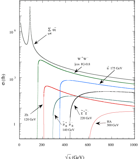
The physics programme described above demands a large amount of integrated luminosity for collisions in the energy range between 90 GeV and 1 TeV. The distribution of luminosity over this energy range will be driven by the physics scenario realised by Nature but it is obvious that independent of any scenario a few ab-1 will be required. Most of the interesting cross sections are of a size typical for the electroweak scale (see Fig. 1), for instance 100 fb for + light Higgs at 500 GeV centre of mass energy ( 200 fb at 350 GeV), and event rates in identified channels will need to be measured to a few percent if the profile is to be established unambiguously.
Important topics which motivate running at 800 GeV have lower cross sections and require even more integrated luminosity, typically for the measurement of the top-Higgs Yukawa coupling or to see the effects of new physics in strong scattering. Supersymmetry, if present, requires the highest possible energy to reach as many sparticles as possible, and high luminosity to scan production thresholds in order to measure their masses precisely. A typical scan requires some 100 fb-1.
The absolute luminosity delivered by the machine can be measured to a precision of 0.1% using the high cross section QED process of Bhabha scattering in the forward region. This is much better than the statistical precision in most physics channels, except for the GigaZ studies.
The beam-beam interaction at the interaction point will be very intense. This leads to a focusing of the bunches resulting in a luminosity enhancement factor of 2. On the other hand beamstrahlung spreads the luminosity spectrum towards lower centre of mass energies. However, about 60% of the total luminosity is still produced at energies higher than 99.5% of the nominal centre of mass energy. For many analyses like threshold scans or high precision measurements in the continuum a good knowledge of the luminosity spectrum is required. This spectrum can be measured from the acolinearity of Bhabha events in the forward region. In the same analysis also the beam energy spread can be measured. The precision with which the beamstrahlung and the beamspread can be measured is good enough that it will not affect any physics analysis.
For several measurements, in particular threshold scans, the absolute energy of the TESLA beams will be determined and monitored with a special spectrometer which can give .
SLC demonstrated the power of using polarised electrons in electroweak studies, and the same technologies will be available to TESLA. Throughout these studies we assume that 80% electron polarisation can be achieved. In a number of analyses, especially for supersymmetry, positron polarisation will also be important. An outline design exists for the production of 45 to 60% polarised positrons. The expected precision for the measurement of the polarisation is 0.5%, sufficient for most analyses. For high precision analyses like at the GigaZ positron polarisation is essential.
The range of physics to be done at TESLA can be significantly extended by operating the machine either as an collider, or with one or both of the beams converted to real high energy photons by Compton back-scattering of laser light from the incoming bunches. The and modes need a non-zero beam-crossing angle, which should be foreseen in the layout of the intersection region for a second collision point.
Many of the feasibility studies presented here have been carried out either with full simulation of the TESLA detector or with a fast simulation, tuned by comparison with the full simulation. The physics processes have been simulated with the full suite of available Monte Carlo generators, some of which now include beam polarisation. The experimental precision which TESLA can achieve must be matched by the theoretical calculations. A continued programme of studies is needed to improve precision on higher order corrections and to understand the indirect contributions from new physics.
4 Conclusions
This volume describes the most likely physics scenarios to be explored at TESLA and describes a detector optimised to carry out that programme. It justifies an immediate commitment to the construction of the collider in its mode, going up to 500 GeV in the centre of mass initially, with a detector that can be designed and built using existing technologies assisted by some well defined R&D.
Increasing the centre of mass energy to 800 GeV (or higher, if the technology will allow) brings important physics benefits and should be regarded as an essential continuation of the programme. The detector can cope easily with this increase.
To carry out the programme the collider must achieve high luminosity and the electron beam must be polarised. Polarisation of the positron beam will also be very useful.
When TESLA has completed its programme of precision measurements at high energies up to 800 GeV, matching improvements will be demanded on some of the electroweak parameters measured at LEP and SLC. The TESLA design should make provision for the possibility of high luminosity running at these low energies (90 to 200 GeV, the GigaZ option).
The other options for colliding beams at TESLA (, or ), add important extra components to the physics programme. Making two polarised electron beams is not difficult. The “photon collider” is more of a challenge, but space should be left in the TESLA layout for a second interaction region with non-zero beam crossing angle where a second detector could be added, either to allow for and or to give a second facility for physics.
The present status of the Standard Model could not have been achieved without inputs from both hadron and electron accelerators and colliders. This should continue into the era of TESLA and the LHC; the physics programme of TESLA is complementary to that of the LHC, they both have complementary strengths and both are needed. TESLA, with its high luminosity over the whole range of energies from 90 GeV to 1 TeV, will make precise measurements of the important quantities, masses, couplings, branching ratios, which will be needed to reveal the origin of electroweak symmetry breaking and to understand the new physics, whatever it will be. There is no scenario in which no new signals would be observed.
In the most likely scenarios with a light Higgs boson the linear collider’s unique ability to perform a comprehensive set of clean precision measurements will allow TESLA to establish the theory unequivocally. In the alternative scenario where the electroweak bosons interact strongly at high energies, TESLA will map out the threshold region of these new interactions. In supersymmetric theories the great experimental potential of the machine will allow us to perform extrapolations to scales near the fundamental Planck scale where particle physics and gravity are linked – a unique opportunity to explore the physics area where all four fundamental forces of Nature will unify.
References
-
[1]
E. Accomando et al. ECFA/DESY LC Physics Working Group,
Phys. Rep. 299:1, 1998;
hep-ph/9705442;
H.Murayama and M.E. Peskin, Ann. Rev. Nucl. Part. Sci. 46:553, 1996. - [2] Conceptual Design of a 500 GeV Linear Collider with Integrated X-ray Laser Facility. editors R. Brinkmann, G. Materlik, J. Rossbach, and A. Wagner, DESY 1997-048, ECFA 1997-182.
-
[3]
Proceedings, Collisions at 500 GeV: The Physics Potential,
Munich–Annecy–Hamburg 1991/93, DESY 92-123A+B, 93-123C,
editor P.M. Zerwas;
Proceedings, Collisions at TeV Energies: The Physics Potential, Annecy–Gran Sasso–Hamburg 1995, DESY 96-123D, editor P.M. Zerwas;
Proceedings, Linear Colliders: Physics and Detector Studies, Frascati – London – München – Hamburg 1996, DESY 97-123E, editor R. Settles. -
[4]
Proceedings, Physics and Experiments with
Linear Colliders, Saariselkä 1991, editors R. Orava,
P. Eerola and M. Nordberg (World Scientific 1992);
Proceedings, Physics and Experiments with Linear Colliders, Waikoloa/Hawaii 1993, editors F. Harris, S. Olsen, S. Pakvasa, X. Tata (World Scientific 1993);
Proceedings, Physics and Experiments with Linear Colliders, Morioka 1995, editors A. Miyamoto, Y. Fujii, T. Matsui, S. Iwata (World Scientific 1996);
Proceedings, Physics and Experiments with Future Linear Colliders, Sitges 1999, editors E. Fernandez, A. Pacheo, Universitat Autònoma de Barcelona, 2000;
Proceedings, International Linear Collider Workshop LCWS2000, Fermilab 2000, American Institute of Physics, to be published. http://www-lc.fnal.gov/lcws2000.
Chapter 1 Higgs Physics
The fundamental particles: leptons, quarks and heavy gauge bosons, acquire mass through their interaction with a scalar field of non-zero field strength in its ground state [2, 3]. To accommodate the well–established electromagnetic and weak phenomena, the Higgs mechanism requires the existence of at least one weak isodoublet scalar field. After absorbing three Goldstone modes to build up the longitudinal polarisation states of the bosons, one degree of freedom is left over, corresponding to a real scalar particle. The discovery of this Higgs boson and the verification of its characteristic properties is crucial for the establishment of the theory of the electroweak interactions, not only in the canonical formulation, the Standard Model (SM) [4], but also in supersymmetric extensions of the SM [5, 6].
If a Higgs particle exists in Nature, the accurate study of its production and decay properties in order to establish experimentally the Higgs mechanism as the mechanism of electroweak symmetry breaking can be performed in the clean environment of linear colliders [7]. The study of the profile of the Higgs particles will therefore represent a central theme of the TESLA physics programme.
In Sections 1 and 2 we review the main scenarios considered in this study and their implications for the Higgs sector in terms of the experimental Higgs signatures. These scenarios are the Standard Model (SM), its minimal supersymmetric extension (MSSM) and more general supersymmetric extensions. The expected accuracies for the determination of the Higgs boson production and decay properties are then presented in Section 2 for the SM Higgs boson, in Section 3 for supersymmetric Higgs bosons and in Section 4 in extended models together with a discussion of their implications for the Higgs boson profile and its nature. Finally the complementarity of the TESLA potential to that of the LHC is discussed in Section 5.
1 Higgs Boson Phenomenology
1 The Standard Model
In the SM the Higgs sector consists of one doublet of complex scalar fields. Their self–interaction leads to a non-zero field strength GeV of the ground state, inducing the breaking of the electroweak symmetry down to the electromagnetic symmetry. Among the four initial degrees of freedom, three will be absorbed in the and boson states and the remaining one corresponds to the physical particle [2]. In addition, the scalar doublet couples to fermions through Yukawa interactions which, after electroweak symmetry breaking, are responsible for the fermion masses. The couplings of the Higgs boson to fermions and gauge bosons are then proportional to the masses and of these particles and completely determined by known SM parameters:
| (1) |
Constraints on the Higgs boson mass
The only unknown parameter in the SM Higgs sector is the Higgs boson mass, . Its value is a free parameter of the theory. However, there are several theoretical and experimental indications that the Higgs boson of the SM should be light. In fact, this conclusion holds quite generally.
 |
 |
For large values of the Higgs boson mass, , the electroweak gauge bosons would have to interact strongly to insure unitarity in their scattering processes and perturbation theory would not be valid anymore. Imposing the unitarity requirement in the elastic scattering of longitudinal bosons at high–energies, for instance, leads to the bound GeV at the tree level [10].
The strength of the Higgs self-interaction is determined by the Higgs boson mass itself at the scale which characterises the spontaneous breaking of the electroweak gauge symmetry. As the energy scale is increased, the quartic self-coupling of the Higgs field increases logarithmically, similarly to the electromagnetic coupling in QED. If the Higgs boson mass is small, the energy cut-off , at which the coupling diverges, is large; conversely, if the Higgs boson mass is large, this becomes small. The upper band in Fig. 1 a) shows the upper limit on the Higgs boson mass as a function of [11]. It has been shown in lattice analyses, which account properly for the onset of the strong interactions in the Higgs sector, that this condition leads to an estimate of about 700 GeV for the upper limit on [12]. However, if the Higgs mass is less than 180 to 200 GeV, the SM can be extended up to the grand unification scale, GeV, or the Planck scale, GeV, while all particles remain weakly interacting [an hypothesis which plays a key role in explaining the experimental value of the mixing parameter ].
Lower bounds on can be derived from the requirement of vacuum stability. Indeed, since the coupling of the Higgs boson to the heavy top quark is fairly large, corrections to the Higgs potential due to top quark loops can drive the scalar self–coupling to negative values, leading to an unstable electroweak vacuum. These loop contributions can only be balanced if is sufficiently large [13]. Based on the triviality and the vacuum stability arguments, the SM Higgs boson mass is expected in the window GeV [8] for a top mass value of about 175 GeV, if the SM is extended to the GUT scale (see Fig. 1 a).
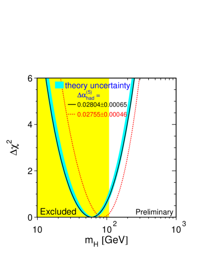
The SM Higgs contribution to the electroweak observables, mainly through corrections of the and propagators, provides further information on its mass. While these corrections only vary logarithmically, , the accuracy of the electroweak data obtained at LEP, SLC and the Tevatron provides sensitivity to . The most recent analysis [9] yields GeV, corresponding to a 95% CL upper limit of 162 GeV. This result depends on the running of the fine-structure constant . Recent improved measurements of in the region between 2 and 5 GeV [14] which are compatible with QCD–based calculations [15] yield GeV corresponding to an upper limit of 206 GeV (see Fig. 1 b). Even using more conservative estimates on the theoretical errors [16], the upper limit on the Higgs boson mass is well within the reach of a 500 GeV linear collider.
Since this result is extracted in the framework of the SM, it can be considered as an effective low-energy approximation to a more fundamental underlying theory. It is interesting to verify how this constraint on may be modified by the effect of new physics beyond the SM. This new physics can be parameterised generically, by extending the SM Lagrangian with effective operators of mass dimension five and higher, weighted by inverse powers of a cut-off scale , representing the scale of new physics. In this approach, the SM result corresponds to . By imposing the necessary symmetry properties on these operators and by fixing their dimensionless coefficients to be , compatibility with the electroweak precision data can be preserved only with 400 GeV, if the operators are not restricted to an unplausibly small set [17]. Though slightly above the SM limit, the data nevertheless require a light Higgs boson even in quite general extended scenarios.
Direct searches for the Higgs boson at LEP yield a lower bound of GeV at the 95% confidence level [18]. The LEP collaborations have recently reported a excess of events beyond the expected SM background in the combination of their Higgs boson searches [18]. This excess is consistent with the production of a SM–like Higgs boson with a mass GeV.
In summary, the properties of the SM Higgs sector and the experimental data from precision electroweak tests favour a light Higgs boson, as the manifestation of symmetry breaking and mass generation within the Higgs mechanism.111For comments on no–Higgs scenarios and their theoretically very complex realisations see Section 3 on strong WW interactions.
Higgs boson production processes
The main production mechanism of this SM Higgs boson in collisions at TESLA are the Higgs-strahlung process [19], , and the fusion process [20], ; Fig. 2. The cross section for the Higgs-strahlung process scales as and dominates at low energies:
| (2) |
where , and . The cross–section for the fusion process [20], , rises and dominates at high energies:
| (3) |

The fusion mechanism, , also contributes to Higgs production, with a cross section suppressed by an order of magnitude compared to that for fusion, due to the ratio of the CC to NC couplings, . In contrast to Higgs-strahlung and fusion, this process is also possible in collisions with approximately the same total cross section as in collisions.

The cross–sections for the Higgs-strahlung and the fusion processes are shown in Fig. 3 for three values of .
At GeV, a sample of 80.000 Higgs bosons is produced, predominantly through Higgs-strahlung, for GeV with an integrated luminosity of 500 fb-1, corresponding to one to two years of running. The Higgs-strahlung process, , with , offers a very distinctive signature (see Fig. 4) ensuring the observation of the SM Higgs boson up to the production kinematical limit independently of its decay (see Table 1). At GeV, the Higgs-strahlung and the fusion processes have approximately the same cross–sections, (50 fb) for 100 GeV 200 GeV.
| (GeV) | = 350 GeV | 500 GeV | 800 GeV |
|---|---|---|---|
| 120 | 4670 | 2020 | 740 |
| 140 | 4120 | 1910 | 707 |
| 160 | 3560 | 1780 | 685 |
| 180 | 2960 | 1650 | 667 |
| 200 | 2320 | 1500 | 645 |
| 250 | 230 | 1110 | 575 |
| Max (GeV) | 258 | 407 | 639 |
At a collider, Higgs bosons can be produced in the resonant s–channel process which proceeds predominantly through a loop of bosons and top quarks [21]. This process provides the unique opportunity to measure precisely the di–photon partial width of the Higgs boson which represents one of the most important measurements to be carried out at a collider. Deviations of from its predicted SM value are a probe of any new charged heavy particle exchanged in the loop such as charged Higgs bosons and supersymmetric particles even if they are too heavy to be directly observed at TESLA or the LHC. The large backgrounds from the continuum process are theoretically and experimentally under control [22, 23].
Higgs boson decays
In the SM, the Higgs boson branching ratios are completely determined [24], once the Higgs boson mass is fixed. For values of the Higgs boson mass in the range GeV, the Higgs boson dominantly decays to fermion pairs, in particular final states since the Higgs fermion couplings are proportional to the fermion masses. The partial width for a decay of the SM Higgs boson into a fermion pair is given by:
| (4) |
with for leptons (quarks). For , the decays and remain significantly suppressed compared to but they are important to test the relative Higgs couplings to up-type and down-type fermions and the scaling of these couplings with the fermion masses. The precise value of the running quark mass at the Higgs boson scale represents a significant source of uncertainty in the calculation of the rates for these decays. QCD corrections to the hadronic decays, being quite substantial, introduce an additional uncertainty. At present, the -quark mass and the uncertainties limit the accuracy for rate predictions for the and channels to about and respectively. Improvements on and , possibly by a factor , can be envisaged after the study of the data on decays from the factories and the LHC. On the contrary, the and predictions can be obtained with accuracies comparable to, or better than, the experimental uncertainties discussed later in this chapter.
Above the threshold and except in a mass range above the threshold, the Higgs boson decays almost exclusively into the or channels, with widths
| (5) |

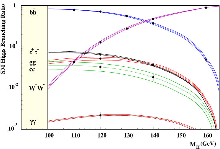
Decays into pairs, with one of the two gauge bosons being virtual, become comparable to the mode at GeV. The Higgs boson branching ratios are shown in Fig. 5 a) as a function of . QCD corrections to the hadronic decays have been taken into account as well as the virtuality of the gauge bosons, and of the top quarks. The top quark and boson mediated loop decays into and final states have small branching ratios, reaching a maximum of at 125 and 145 GeV, respectively. However, they lead to clear signals and are interesting because they are sensitive to new heavy particles.
By adding up all possible decay channels, we obtain the total Higgs boson decay width, as shown in Fig. 5 b) for 175 GeV. Up to masses of 140 GeV, the Higgs particle is very narrow, 10 MeV. After opening the mixed real/virtual gauge boson channels, the state becomes rapidly wider, reaching 1 GeV at the threshold.
2 Supersymmetric Extension of the Standard Model
Several extensions of the SM introduce additional Higgs doublets and singlets. In the simplest of such extensions the Higgs sector consists of two doublets generating five physical Higgs states: , , and . The and states are even and the is odd. Besides the masses, two mixing angles define the properties of the Higgs bosons and their interactions with gauge bosons and fermions, namely the ratio of the vacuum expectation values and a mixing angle in the neutral -even sector. These models are generally referred to as 2HDM and they respect the SM phenomenology at low energy. In particular, the absence of flavour changing neutral currents is guaranteed by either generating the mass of both up- and down-like quarks through the same doublet (Model I) or by coupling the up-like quarks to the first doublet and the down-like quarks to the second doublet (Model II). Two Higgs field doublets naturally arise in the context of the minimal supersymmetric extension of the SM (MSSM).
One of the prime arguments for introducing Supersymmetry [25, 5] is the solution of the hierarchy problem. By assigning fermions and bosons to common multiplets, quadratically divergent radiative corrections to the Higgs boson mass can be cancelled in a natural way [3, 6] by adding up bosonic and opposite–sign fermionic loops. As a result of the bosonic–fermionic supersymmetry, Higgs bosons can be retained as elementary spin–zero particles with masses close to the scale of the electroweak symmetry breaking even in the context of very high Grand Unification scales. These supersymmetric theories are strongly supported by the highly successful prediction of the electroweak mixing angle: , . In addition, the breaking of the electroweak symmetry may be generated in supersymmetric models in a natural way via radiative corrections associated with the heavy top quark. The MSSM serves as a useful guideline into this area, since only a few phenomena are specific to this model and many of the characteristic patterns are realized also in more general extensions.
The Higgs spectrum in the MSSM
In the MSSM, two doublets of Higgs fields are needed to break the electroweak symmetry, leading to a Higgs spectrum consisting of five particles [26]: two –even bosons and , a –odd boson and two charged particles . Supersymmetry leads to several relations among these parameters and, in fact, only two of them are independent at the tree level. These relations impose a strong hierarchical structure on the mass spectrum and some of which are, however, broken by radiative corrections.
The leading part of these radiative corrections [27, 28, 29] to the Higgs boson masses and couplings grows as the fourth power of the top quark mass and logarithmically with the SUSY scale or common squark mass [27]; mixing in the stop sector has also to be taken into account. The radiative corrections push the maximum value of the lightest boson mass upwards by several ten GeV [28, 29]; a recent analysis, including the dominant two–loop contributions gives an upper bound GeV [30]; c.f. Fig. 6 a) where the MSSM Higgs masses are shown for TeV and This upper bound is obtained for large values of TeV and and crucially depends on the value of the top quark mass. The precise determination of possible at TESLA is instrumental for precision physics in the MSSM Higgs sector.


|
The couplings of the MSSM Higgs bosons to fermions and gauge bosons depend strongly on the angles and . The pseudo-scalar and charged Higgs boson couplings to down (up) type fermions are (inversely) proportional to ; the pseudo-scalar has no tree level couplings to two gauge bosons. For the –even Higgs bosons, the couplings to down (up) type fermions are enhanced (suppressed) compared to the SM Higgs couplings [for values ]; the couplings to gauge bosons are suppressed by factors (see Tab. 2 and Fig. 6 b)).
If is very close to its upper limit for a given value of , the couplings of the boson to fermions and gauge bosons are SM like, while the couplings of the heavy boson become similar to that of the pseudoscalar boson; Tab. 2. This decoupling limit [31] is realized when and in this regime, the and bosons are almost degenerate in mass.
MSSM Higgs production
In addition to the Higgs-strahlung and fusion production processes for the –even Higgs particles and , and , the associated pair production process, , also takes place in the MSSM or in two–Higgs doublet extensions of the SM. The pseudoscalar cannot be produced in the Higgs-strahlung and fusion processes to leading order. The cross sections for the Higgs-strahlung and pair production processes can be expressed as [32]
| (6) |
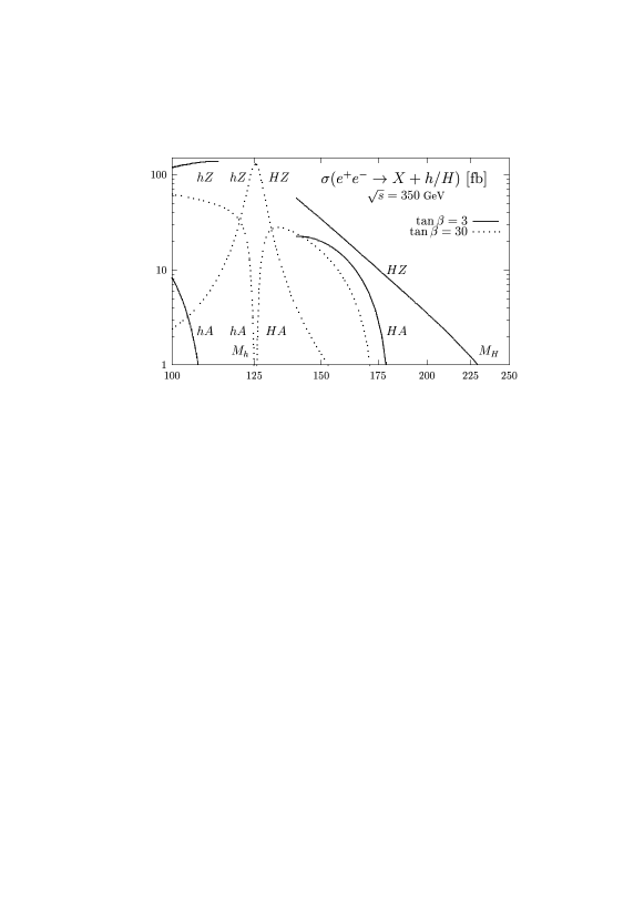
where is the SM cross section for Higgs-strahlung and the coefficient , given by ( is defined below eq. 2 and or , respectively) accounts for the suppression of the –wave cross sections near threshold. Representative examples of the cross sections in these channels are shown as a function of the Higgs masses in Fig.7 at a c.m. energy GeV for and 30. The cross sections for the Higgs-strahlung and for the pair production, likewise the cross sections for the production of the light and the heavy neutral Higgs bosons and , are mutually complementary to each other, coming either with coefficients or . As a result, since is large, at least the lightest –even Higgs boson must be detected. For large values, the main production mechanism for the heavy neutral Higgs bosons is the associated process when kinematically allowed; the cross section is shown for a c.m. energy GeV in Fig. 8.
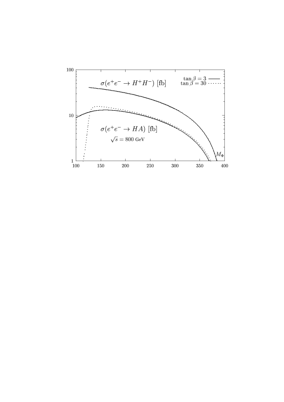
Charged Higgs bosons, if lighter than the top quark, can be produced in top decays, , with a branching ratio varying between and in the kinematically allowed region. Charged Higgs particles can also be directly pair produced in collisions, , with a cross section which depends mainly on the mass [32]. It is of (50 fb) for small masses at GeV, but it drops very quickly due to the –wave suppression near the threshold ( see Fig. 8). For GeV, the cross section falls to a level of fb, which for an integrated luminosity of corresponds to events.
The MSSM Higgs bosons can also be produced in collisions, and , with favourable cross sections [33]. For the neutral and bosons, this mode is interesting since one can probe higher masses than at the collider, GeV for a 500 GeV initial c.m. energy. Furthermore, an energy scan could resolve the small and mass difference near the decoupling limit.
MSSM Higgs decays
The decay pattern of the Higgs bosons in the MSSM [34] is more complicated than in the SM and depends strongly on the value of ( see Fig. 9).

The lightest neutral boson will decay mainly into fermion pairs since its mass is smaller than 130 GeV. This is, in general, also the dominant decay mode of the pseudo-scalar boson . For values of much larger than unity, the main decay modes of the three neutral Higgs bosons are decays into and pairs; the branching ratios being of order and , respectively. For large masses, the top decay channels open up, yet for large this mode remains suppressed. If the masses are high enough, the heavy boson can decay into gauge bosons or light boson pairs and the pseudo-scalar particle into final states; these decays are strongly suppressed for . The charged Higgs particles decay into fermions pairs: mainly and final states for masses, respectively, above and below the threshold. If allowed kinematically, the bosons decay also into final states. Adding up the various decay modes, the Higgs bosons widths remain narrow, being of order 10 GeV even for large masses. However, the total width of the boson may become much larger than that of the SM boson for large values.
Other possible decay channels for the MSSM bosons, in particular the heavy and states, are decays into supersymmetric particles [35]. In addition to light sfermions, decays into charginos and neutralinos could eventually be important if not dominant. Decays of the lightest boson into the lightest neutralinos (LSP) or sneutrinos can be also important, exceeding 50% in some parts of the SUSY parameter space, in particular in scenarios where the gaugino and sfermion masses are not unified at the GUT scale [36]. These decays strongly affect experimental search techniques. In particular, invisible neutral Higgs decays could jeopardise the search for these states at hadron colliders where these modes are very difficult to detect.
Non–minimal SUSY extensions
A straightforward extension of the MSSM is the addition of an iso–singlet scalar field [37, 38]. This next–to-minimal extension of the SM or (M+1)SSM has been advocated to solve the so–called problem, i.e. to explain why the Higgs–higgsino mass parameter is of . The Higgs spectrum of the (M+1)SSM includes in addition one extra scalar and pseudo-scalar Higgs particles. The neutral Higgs particles are in general mixtures of the iso–doublets, which couple to bosons and fermions, and the iso–singlet, decoupled from the non–Higgs sector. Since the two trilinear couplings involved in the potential, and , increase with energy, upper bounds on the mass of the lightest neutral Higgs boson can be derived, in analogy to the SM, from the assumption that the theory be valid up to the GUT scale: GeV [38]. If is (nearly) pure iso–scalar and decouples, its role is taken by the next Higgs particle with a large isodoublet component, implying the validity of the mass bound again.
The couplings of the –even neutral Higgs boson to the boson, , are defined relative to the usual SM coupling. If is primarily isosinglet, the coupling is small and the particle cannot be produced by Higgs-strahlung. However, in this case is generally light and couples with sufficient strength to the boson; if not, plays this role. Thus, despite the additional interactions, the distinct pattern of the minimal extension remains valid also in this SUSY scenario [39].
In more general SUSY scenarios, one can add an arbitrary number of Higgs doublet and/or singlet fields without being in conflict with high precision data. The Higgs spectrum becomes then much more complicated than in the MSSM, and much less constrained. However, the triviality argument always imposes a bound on the mass of the lightest Higgs boson of the theory as in the case of the (M+1)SSM. In the most general SUSY model, with arbitrary matter content and gauge coupling unification near the GUT scale, an absolute upper limit on the mass of the lightest Higgs boson, GeV, has been recently derived [40].
Even if the Higgs sector is extremely complicated, there is always a light Higgs boson which has sizeable couplings to the boson. This Higgs particle can thus be produced in the Higgs-strahlung process, “”, and using the missing mass technique this “” particle can be detected independently of its decay modes [which might be rather different from those of the SM Higgs boson]. Recently a powerful “no lose theorem” has been derived [41]: a Higgs boson in SUSY theories can always be detected at a 500 GeV collider with a luminosity of fb-1 in the Higgs-strahlung process, regardless of its decays and of the complexity of the Higgs sector of the theory.
2 Study of the Higgs Boson Profile
1 Mass measurement
Since the SM Higgs boson mass is a fundamental parameter of the theory, the measurement is a very important task. Once is fixed, the profile of the Higgs particle is uniquely determined in the SM. In theories with extra Higgs doublets, the measurement of the masses of the physical boson states is crucial to predict their production and decay properties as a function of the remaining model parameters and thus perform a stringent test of the theory.
At the linear collider, can be measured best by exploiting the kinematical characteristics of the Higgs-strahlung production process , where the boson can be reconstructed in both its hadronic and leptonic decay modes [42].
For the case of SM-like couplings, a neutral Higgs boson with mass 130 GeV decays predominantly to . Thus, production gives four jet and two jet plus two lepton final states.
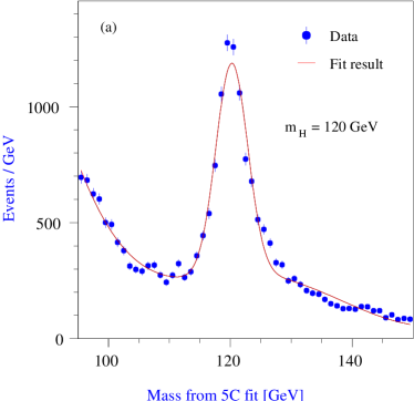
In the four–jet channel, the Higgs boson is reconstructed through its decay to with the boson decaying into a pair. The Higgs boson mass determination relies on a kinematical 5-C fit imposing energy and momentum conservation and requiring the mass of the jet pair closest to the mass to correspond to . This procedure gives a mass resolution of approximately 2 GeV for individual events. A fit to the resulting mass distribution, shown in Fig. 1 a), gives an expected accuracy of 50 MeV [43] for GeV and an integrated luminosity of 500 fb-1 at GeV.
 |
 |
 |
 |
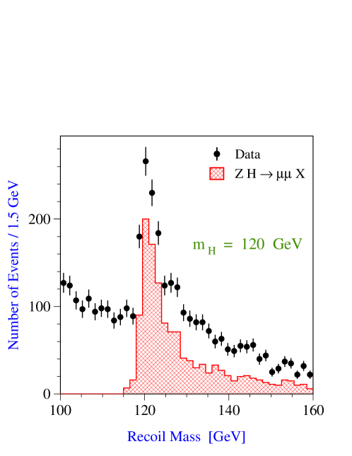
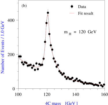
The leptonic decays and offer a clean signature in the detector, and the lepton momenta can be measured with high accuracy in the large tracking volume of the TESLA detector. In the case of backgrounds are larger than in the channel due to large cross section for Bhabha scattering. Bhabha events with double ISR can be efficiently suppressed using a likelihood technique [44]. In order to further improve the resolution of the recoil mass, a vertex constraint is applied in reconstructing the lepton trajectories. Signal selection efficiencies in excess of 50% are achieved for both the electron and the muon channels, with a recoil mass resolution of 1.5 GeV for single events. The recoil mass spectrum is fitted with the Higgs boson mass, the mass resolution and the signal fraction as free parameters. The shape of the signal is parametrised using a high statistics simulated sample including initial state radiation and beamstrahlung effects while the background shape is fitted by an exponential. The shape of the luminosity spectrum can be directly measured, with high accuracy, using Bhabha events. The estimated precision on is 110 MeV for a luminosity of 500 fb-1 at = 350 GeV, without any requirement on the nature of the Higgs boson decays. By requiring the Higgs boson to decay hadronically and imposing a 4-C fit, the precision can be improved to 70 MeV [43] (see Fig. 1 b)).
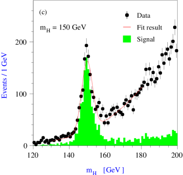
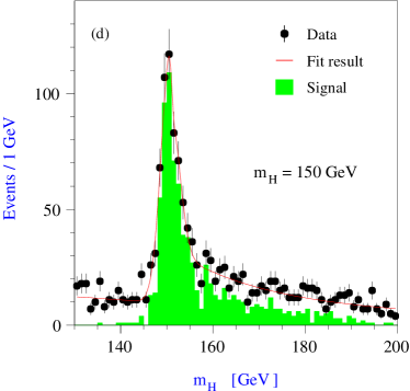
As increases above 130 GeV, the channel becomes more important and eventually dominates for masses from 150 GeV up to the threshold. In this region, the Higgs boson decay can be fully reconstructed by selecting hadronic decays leading to six jet (Fig. 1 c)) and four jet plus two leptons (Fig. 1 d)) final states [43].
The recoil mass technique, insensitive to the actual Higgs boson decay channel, is also exploited and provides a comparable mass determination accuracy, the smaller statistics being compensated by the better mass resolution.
Table 1 summarises the expected accuracies on the Higgs boson mass determination. If the Higgs boson decays predominantly into invisible final states, as predicted by some models mentioned earlier, but its total width remains close to that predicted by the SM, the recoil mass technique is still applicable and determines the achievable accuracy on the mass determination.
| Channel | ||
| (GeV) | (MeV) | |
| 120 | 70 | |
| 120 | 50 | |
| 120 | Combined | 40 |
| 150 | Recoil | 90 |
| 150 | 130 | |
| 150 | Combined | 70 |
| 180 | Recoil | 100 |
| 180 | 150 | |
| 180 | Combined | 80 |
2 Couplings to massive gauge bosons
The couplings of the Higgs boson to massive gauge bosons is probed best in the measurement of the production cross–section for Higgs-strahlung ( probing ) and fusion ( probing ). The measurement of these cross–sections is also needed to extract the Higgs boson branching ratios from the observed decay rates and provide a determination of the Higgs boson total width when matched with the branching ratio as discussed later.
The cross–section for the Higgs-strahlung process can be measured by analysing the mass spectrum of the system recoiling against the boson as already discussed in Section 1. This method provides a cross–section determination independent of the Higgs boson decay modes. From the number of signal events fitted to the di-lepton recoil mass spectrum, the Higgs-strahlung cross–section is obtained with a statistical accuracy of 2.8%, combining the and channels. The systematics are estimated to be 2.5%, mostly due to the uncertainties on the selection efficiencies and on the luminosity spectrum [42]. The results are summarised in Table 2.
| Fit | (stat) | |
|---|---|---|
| (GeV) | (fb) | |
| 120 | 5.300.13(stat)0.12(syst) | 0.025 |
| 140 | 4.39 0.12(stat)0.10(syst) | 0.027 |
| 160 | 3.60 0.11(stat)0.08(syst) | 0.030 |
The cross–section for fusion can be determined in the final state, where these events can be well separated from the corresponding Higgs-strahlung final state, , and the background processes by exploiting their different spectra for the invariant mass (Fig. 2). There could be serious contamination of events from overlapping events, but the good spatial resolution of the vertex detector will make it possible to resolve the longitudinal displacement of the two separate event vertices, within the TESLA bunch length [45]. The precision to which the cross–section for fusion can be measured with 500 at GeV is given in Table 3 [46]. Further, by properly choosing the beam polarisation configurations, the relative contribution of Higgs-strahlung and fusion can be varied and systematics arising from the contributions to the fitted spectrum from the two processes and their effect can be kept smaller than the statistical accuracy [47].
 |
 |
An accurate determination of the branching ratio for the decay can be obtained in the Higgs-strahlung process by analysing semi-leptonic [48] and fully hadronic [49] decays. The large and backgrounds can be significantly reduced by imposing the compatibility of the two hadronic jets with the mass and that of their recoil system with the Higgs boson mass. Further background suppression is ensured by an anti- tag requirement that rejects the remaining and events. The residual background with one off-shell can be further suppressed if the electron beam has right-handed polarisation.
| Channel | = 120 GeV | 140 GeV | 160 GeV |
|---|---|---|---|
| 0.025 | 0.027 | 0.030 | |
| 0.028 | 0.037 | 0.130 | |
| 0.051 | 0.025 | 0.021 | |
| 0.169 |
3 Coupling to photons
The Higgs effective coupling to photons is mediated by loops. These are dominated, in the SM, by the contributions from the boson and the top quark but are also sensitive to any charged particles coupling directly to the Higgs particle and to the photon.
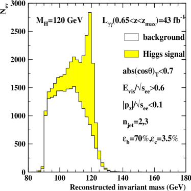
At the collider, the process has a very substantial cross–section. The observation of the Higgs signal through its subsequent decay requires an effective suppression of the large non–resonant and backgrounds. Profiting from the effective / jet flavour discrimination of the TESLA detector, it is possible to extract the Higgs signal with good background rejection (see Fig. 3 a)). Assuming = 120 GeV and an integrated luminosity of 43 fb-1 in the hard part of the spectrum, an accuracy of about 2% on can be achieved [23, 50] (see Part VI, Chapter 1.).
 |
 |
The Higgs coupling to photons is also accessible through the decay. The measurement of its branching ratio together with the production cross–section at the TESLA collider is important for the extraction of the Higgs boson width. The branching ratio analysis is performed in both the and the + jets final states, corresponding to the sum of the fusion, , and , respectively [51]. The most important background in both channels comes from the double-bremsstrahlung process. This background and the smallness of the partial decay width make the analysis a considerable experimental challenge. However the signal can be discriminated from this irreducible background, since the photons in the signal have a spectrum peaked at high energy and rather isotropic production contrary to the background process which has photons produced at large polar angles and with lower energies. Efficiency values in the range 50% to 65% are obtained for the and final states. Combining both channels, the relative accuracy for the measurement of for GeV is 26% (23%), for an integrated luminosity of 500 fb-1 at = 350 GeV (500 GeV). For 1000 fb-1, an accuracy of 18% (16%) can be reached (see Fig. 3 b)).
4 The Higgs boson total decay width
The SM Higgs boson total width, , is extremely small for light mass values and increases rapidly once the and decay channels become accessible, reaching a value of 1 GeV at the threshold. Therefore, for 200 GeV the total decay width becomes directly accessible from the reconstruction of the Higgs boson line-shape. However at the linear collider and for lower masses, it can be obtained semi–directly, in a nearly model–independent way, from the combination of the measurements of a Higgs coupling constant with the corresponding branching ratio.
Absolute measurements of coupling constants can be obtained (i) for through the Higgs-strahlung cross–section, for through (ii) the fusion cross–section or, more model-dependently, (iii) by using the symmetry and, in the collider option, for through (iv) the cross–section for .
For a mass below 160 GeV, the best method is to use the fusion process. Combined with the measurement of the branching ratio for (see section 2) an accuracy ranging from 4% to 13% can be obtained for , as shown in Table 4.
| BR() | = 120 GeV | 140 GeV | 160 GeV | |
|---|---|---|---|---|
| 0.061 | 0.045 | 0.134 | ||
| 0.056 | 0.037 | 0.036 | ||
| 0.23 | - | - |
An alternative method is to exploit the effective coupling through the measurement of the cross–section for using the collider option. This cross–section and hence the partial width can be obtained to 2% accuracy for and to better than 10% for . The derivation of the total width however needs the measurement of the branching ratio as input. As it was shown in Sec. 3, this can only be achieved to 23% precision for 500 fb-1 and thus dominates the uncertainty on the total width reconstructed from the H coupling.
5 Couplings to fermions
The accurate determination of the Higgs couplings to fermions is important as a proof of the Higgs mechanism and to establish the nature of the Higgs boson. The Higgs-fermion couplings being proportional to the fermion masses, the SM Higgs boson branching ratio into fermions are fully determined once the Higgs boson and the fermion masses are fixed.
Deviations of these branching ratios from those predicted for the SM Higgs boson can be the signature of the lightest supersymmetric boson. Higgs boson decays to , like those to , proceed through loops, dominated in this case by the top contribution. The measurements of these decays are sensitive to the top Yukawa coupling in the SM and the existence of new heavy particles contributing to the loops.
The accuracy on the Higgs boson branching ratio measurements at the linear collider has been the subject of several studies [52]. With the high resolution Vertex Tracker, the more advanced jet flavour tagging techniques, the experience gained at LEP and SLC (see Part IV, Chapter 9), and the large statistics available at the TESLA collider, these studies move into the domain of precision measurements.
In the hadronic Higgs boson decay channels at TESLA, the fractions of , and final states are extracted by a binned maximum likelihood fit to the jet flavour tagging probabilities for the Higgs boson decay candidates [53]. The background is estimated over a wide interval around the Higgs boson mass peak and subtracted. It is also possible to study the flavour composition of this background directly in the real data by using the side-bands of the Higgs boson mass peak. The jet flavour tagging response can be checked by using low energy runs at the as well as events at full energy, thus reducing systematic uncertainties from the simulation.
For the case of , a global likelihood is defined by using the response of discriminant variables such as charged multiplicity, jet invariant mass and track impact parameter significance.
These measurements are sensitive to the product . Using the results discussed above for the production cross–sections , the branching ratios can be determined to the accuracies summarised in Table 5 and shown in Fig. 4 [53].
| Channel | = 120 GeV | = 140 GeV | = 160 GeV |
|---|---|---|---|
| 0.024 | 0.026 | 0.065 | |
| 0.083 | 0.190 | ||
| 0.055 | 0.140 | ||
| 0.050 | 0.080 |
6 Higgs top Yukawa coupling
The Higgs Yukawa coupling to the top quark is the largest coupling in the SM ( to be compared with ). If this coupling is directly accessible in the process [54]. This process, with a cross–section of the order of 0.5 fb for GeV at = 500 GeV and 2.5 fb at = 800 GeV, including QCD corrections [55], leads to a distinctive signature consisting of two bosons and four -quark jets.

The experimental accuracy on the determination of the top Yukawa coupling has been studied for = 800 GeV and fb-1 in both the semileptonic and fully hadronic channels [56]. The main sources of efficiency loss are from failures of the jet-clustering and of the -tagging due to hard gluon radiation and to large multiplicities. The analysis uses a set of highly efficient pre-selection criteria and a Neural Network trained to separate the signal from the remaining backgrounds. Because of the large backgrounds, it is crucial that they are well modelled both in normalisation and event shapes. A conservative estimate of 5% uncertainty in the overall background normalisation has been used in the evaluation of systematic uncertainties. For an integrated luminosity of 1000 fb-1 the statistical uncertainty in the Higgs top Yukawa coupling after combining the semileptonic and the hadronic channels is 4.2% (stat). This results in an uncertainty of 5.5% (stat.+syst.) [56] (see Fig. 5).
If , the Higgs top Yukawa couplings can be measured from the branching ratio, similarly to those of the other fermions discussed in the previous section. A study has been performed for the fusion process for 350 GeV 500 GeV at = 800 GeV [57]. The and the backgrounds are reduced by the event selection based on the characteristic event signature with six jets, two of them from a quark, on the missing energy and the mass. Since the S/B ratio is expected to be large, the uncertainty on the top Yukawa coupling is dominated by the statistics and corresponds to 5% (12%) for = 400 (500) GeV for an integrated luminosity of 1000 fb-1 [57].
7 Extraction of Higgs couplings
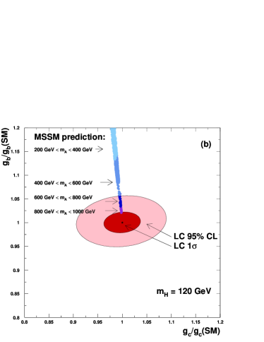
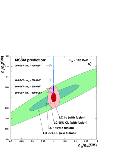
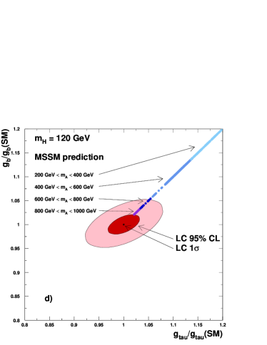
The Higgs boson production and decay rates discussed above, can be used to measure the Higgs couplings to gauge bosons and fermions. After the Higgs boson is discovered, this is the first crucial step in establishing experimentally the Higgs mechanism for mass generation. Since some of the couplings of interest can be determined independently by different observables while other determinations are partially correlated, it is interesting to perform a global fit to the measurable observables and to extract the Higgs couplings in a model–independent way. This method optimises the available information and can take properly into account the experimental correlation between different measurements.
 |
 |
 |
 |
| Coupling | = 120 GeV | 140 GeV |
|---|---|---|
| 0.012 | 0.020 | |
| 0.012 | 0.013 | |
| 0.030 | 0.061 | |
| 0.022 | 0.022 | |
| 0.037 | 0.102 | |
| 0.033 | 0.048 | |
| 0.017 | 0.024 | |
| 0.029 | 0.052 | |
| 0.012 | 0.022 | |
| 0.033 | 0.041 | |
| 0.026 | 0.057 | |
| 0.041 | 0.100 | |
| 0.027 | 0.042 |
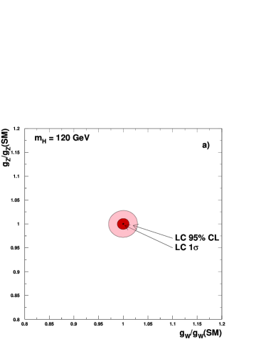
A dedicated program, HFitter [58] has been developed based on the Hdecay [24] program for the calculation of the Higgs boson branching ratios. The following inputs have been used: , , BR(), BR(), BR(), BR(), BR(), BR(), . For correlated measurements the full covariance matrix has been used. The results are given for = 120 GeV and 140 GeV and 500 fb-1. Table 6 shows the accuracy which can be achieved in determining the couplings and their relevant ratios. Fig. 6 shows 1 and 95% confidence level contours for the fitted values of various pairs of ratios of couplings, with comparisons to the sizes of changes expected from the MSSM.
8 Quantum numbers of the Higgs boson
The spin, parity, and charge-conjugation quantum numbers of the Higgs bosons can be determined at TESLA in a model-independent way [59]. The observation of Higgs boson production at the collider or of the decay would rule out and require to be positive.
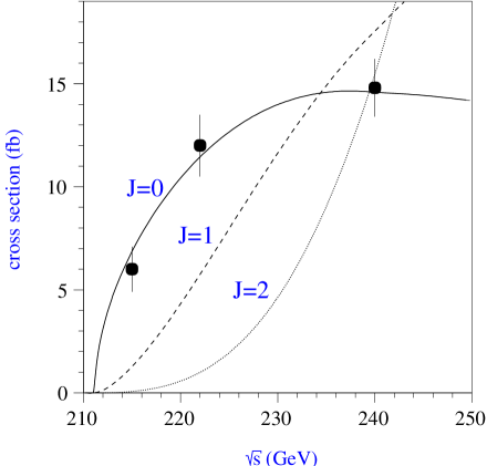
The measurement of the rise of the total Higgs-strahlung cross section at threshold and the angular dependence of the cross–section in the continuum allow and to be uniquely determined.
The threshold rise of the process for a boson of arbitrary spin and normality has been studied in [60]. While for the cross section at threshold rises (see eq. 2), for higher spins the cross section rises generally with higher powers of except for some scenarios with which can be distinguished through the angular dependence in the continuum. A threshold scan with a luminosity of 20 fb-1 at three centre–of–mass energies is sufficient to distinguish the different behaviours (see Fig. 7) [61].
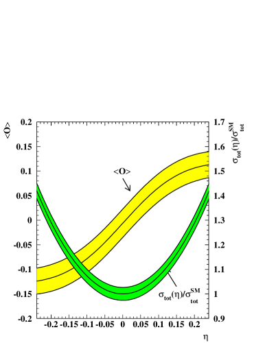
In the continuum, one can distinguish the SM Higgs boson from a -odd state , or a –violating mixture of the two (generically denoted by in the following). The nature of the Higgs bosons can be established by comparing the cross section angular dependence with that of the process, which exhibits a distinctly different angular momentum structure (see Fig. 8 a)) due to the t-channel electron exchange. However, in a general 2HDM model the three neutral Higgs bosons correspond to arbitrary mixtures of eigenstates, and their production and decay exhibit violation. In this case, the amplitude for the Higgs-strahlung process can be described by adding a ZZA coupling with strength to the SM matrix element . In general the parameter can be complex, we assume it to be real in the following. If , we recover the coupling of SM Higgs boson . However, in a more general scenario, need not be loop suppressed as in the MSSM, and it is useful to allow for to be arbitrary in the experimental data analysis. The most sensitive single kinematic variable to distinguish these different contributions to Higgs boson production is the production angle of the boson w.r.t. to the beam axis, in the laboratory frame. The differential cross–section for the process is given by:
where and , and are defined below equation 2. The angular distribution of , , corresponding to transversely polarised bosons, is therefore very distinct from that of in the SM, , for longitudinally polarised bosons in the limit [59]. In the above equation, the interference term, linear in , generates a forward-backward asymmetry, which would represent a distinctive signal of violation, while the term proportional to increases the total cross–section.
 |
 |
The angular distributions of the accompanying decay products are also sensitive to the Higgs boson parity and spin as well as to anomalous couplings [62]. In fact, at high energies, the bosons from are dominantly longitudinally polarised, while those from () are fully (dominantly) transversely polarised [59]. These distributions can be described in terms of the angles and , where is the polar angle between the flight direction of the decay fermion in the -boson rest frame and that of the -boson in the laboratory frame and is the corresponding azimuthal angle w.r.t. the plane defined by the beam axis and the -boson flight direction.
The information carried by these three angular distributions can be analysed using the optimal observable formalism [63], in terms of a single variable defined as the ratio of the -violating contribution to the SM cross–section, . If the Higgs boson production respects symmetry, the expectation value of this –odd observable must vanish, i.e. . Any significant deviation of from 0 implies the existence of violation, independent of the specific model.
This analysis has been performed for = 120 GeV assuming an integrated luminosity of 500 fb-1 at = 350 GeV, following the criteria of the reconstruction discussed above. However, in order not to bias the analysis towards specific Higgs boson decay modes, only cuts on decay products are applied. The resulting sensitivity is shown in Fig. 8 b) for the case of . The accuracy in the determination of , obtained using the expectation value of the optimal observable is 0.038, and it improves to 0.032 when the total cross–section dependence is exploited in addition [64].
| — | 0.5 | 0.5 | |
|---|---|---|---|
| — | 0.6 | 0.6 | |
| — | — | 0.8 | |
| — | — | 0.45 | |
| Re | 0.00055 | 0.00029 | 0.00023 |
| Re | 0.00065 | 0.00017 | 0.00011 |
| Re | 0.01232 | 0.00199 | 0.00036 |
| Re | 0.00542 | 0.00087 | 0.00008 |
| Re | 0.00104 | 0.00097 | 0.00055 |
| Re | 0.00618 | 0.00101 | 0.00067 |
 |
 |
In the effective-Lagrangian approach, the most general coupling can have two more independent –even terms [65]. Similarly, there may also be an effective coupling, generated by two –even and one –odd terms [65] making a total of seven complex couplings, , , , , , , and , where the –odd couplings are indicated by a tilde. With sufficiently high luminosity, accurate helicity and good charge identification and electron and positron beam polarisation it will be possible to determine these couplings from the angular distributions of [47] A global analysis of these angular distributions, based on the optimal observable method [66, 63] and assuming GeV, fb-1, helicity and charge identification efficiencies and , and beam polarisations , gives the results summarised in Table 7 and in Fig. 9 for fixed . The coupling can be determined by repeating the analysis at two different values of , such as 350 GeV and 500 GeV. We observe that the couplings are generally well constrained, even for . The constraints on the couplings may be improved by approximately a factor of 6 through and tagging and by another factor of 1.5 to 10 through beam polarisation.
9 Higgs potential
To establish the Higgs mechanism experimentally in an unambiguous way, the self potential of the Higgs field:
| (1) |
with a minimum at , must be reconstructed. This can be accomplished by measuring the self-couplings of the physical Higgs boson [67, 68] as predicted by the potential:
| (2) |
The coefficient of the bilinear term in the Higgs field defines the mass so that the trilinear and quadrilinear couplings can be predicted unambiguously in the SM.

The trilinear Higgs coupling , in units of , can be measured directly in pair-production of Higgs particles at high-energy colliders [67, 68, 69]. The most interesting process at TESLA centre–of–mass energies is the associated production of two Higgs bosons with a boson, . As evident from Fig. 10, this process is built up by the amplitude involving the trilinear Higgs coupling superimposed on the two other mechanisms which lead to the same final state but do not involve . The cross–section for double Higgs production, which is therefore a binomial in the coupling , is of the order of 0.20 fb for = 120 GeV at = 500 GeV and 0.15 fb at = 800 GeV (see Fig. 11). The quadrilinear Higgs coupling can in principle be measured in triple Higgs boson production, but the cross–section is suppressed by an additional electroweak factor, and is therefore too small to be observable at TESLA energies [68].
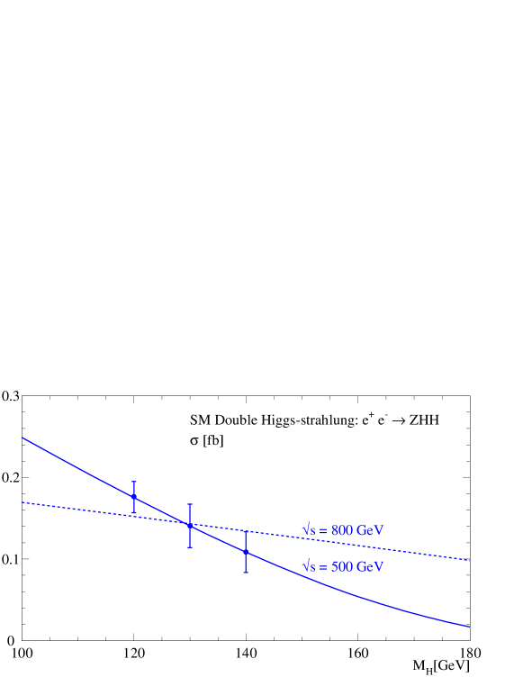
A detailed analysis of the reconstruction of double Higgs-strahlung events has been performed [70]. The large four and six fermion background and the tiny signal cross–section make this analysis a genuine experimental challenge. However, by profiting from the characteristic signature with four jets and a boson, reconstructed either in its leptonic or hadronic decay modes, and from the excellent tagging and energy flow reconstruction capabilities of the TESLA detector (see Part IV, Chapter 9), this process can be isolated from backgrounds.
| (GeV) | 120 | 130 | 140 |
|---|---|---|---|
| 80 | 64 | 44 | |
| Efficiency | 0.43 | 0.43 | 0.39 |
| 0.17 | 0.19 | 0.23 |
In the hadronic channel, after kinematical cuts, the events are forced into six jets and the jet pair most consistent with the hypothesis is identified. In the leptonic channel two identified leptons consistent with a boson are required instead. Then the jets recoiling against the reconstructed boson are required to contain identified b–quarks. With this selection, accuracies of approximately 20% on the cross–section can be obtained for between 120 and 140 GeV and 1000 fb-1 (see Table 8 and Fig. 11). The sensitivity can be further improved when a multi-variable selection based on a neural network is applied, reducing the uncertainty from 17% to 13% for GeV and yielding a signal significance .
The sensitivity to is diluted due to the additional diagrams shown in Fig. 10. Taking this into account, the trilinear Higgs coupling can be obtained at TESLA with a statistical accuracy of 22% for GeV with an integrated luminosity of 1000 fb-1, using the neural network selection [70]. This measurement crucially depends on the high luminosity anticipated for the TESLA operation and the accurate decay reconstruction provided by the optimised detector. It represents an essential element for the reconstruction of the characteristic Higgs potential which leads to the non-zero value of the Higgs field in the vacuum, the physical basis of the Higgs mechanism for breaking the electroweak symmetry and generating the masses of the fundamental particles.
3 Study of SUSY Higgs Bosons
If supersymmetry exists in Nature, a major goal of TESLA will be the measurement of its parameters. In this way, the underlying SUSY-breaking mechanism could be determined and thorough consistency checks of the model itself could be performed. The TESLA potential in the investigations of the supersymmetric particle partners is described in detail in Section 2. Here the perspectives of the study of the extended Higgs sector as predicted in supersymmetry is discussed.
The study of the lightest neutral MSSM Higgs boson follows closely that of the SM-like discussed above, and similar results, in terms of the achievable experimental accuracies, are valid. This light Higgs boson, , can be found at colliders easily. The ability of TESLA to distinguish the SM/MSSM nature of a neutral Higgs boson is discussed below.
In SUSY models, additional decay channels may open for the Higgs bosons if supersymmetric particles exist with light enough masses. The most interesting scenario is that in which the lightest Higgs boson decays in particles escaping detection giving a sizeable decay width. While the Higgs boson observability in the di-lepton recoil mass in the associated production channel is virtually unaffected by this scenario, such an invisible decay width can be measured by comparing the number of events with the sum over the visible decay modes corrected by the branching ratio: BR() ). Using the accuracies on the determination of the individual branching ratios discussed above, the rate for the decay can be determined to better than 20% for BR() 0.05.
1 Study of the , and bosons
A most distinctive feature of extended models such as supersymmetry, or general 2HDM extensions of the SM, is the existence of additional Higgs bosons. Their mass and coupling patterns vary with the model parameters. However in the decoupling limit, the , and bosons are expected to be heavy and to decay predominantly into quarks of the third generation. Establishing their existence and the determination of their masses and of their main decay modes will represent an important part of the TESLA physics programme at centre-of-mass energies exceeding 500 GeV.
For a charged Higgs boson mass larger than 222The case with the decay is discussed in Section 1, the dominant production mode is pair production, with the dominant decay modes being with contributions from and (see Fig. 9). The cross–section depends mainly on the charged Higgs boson mass and is of the order of 15 fb for = 300 GeV at = 800 GeV (see Fig. 8). The radiative corrections do significantly change these results [71].
As an example of the performance of TESLA, a study has been made of the and the , processes with = 300 GeV, = 120 GeV and = 800 GeV [72].
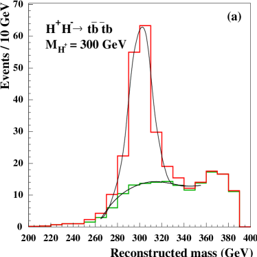 |
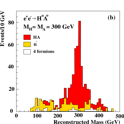 |
In the resulting 8 jet final state with 4 -quark jets it is possible to beat down the backgrounds to a low level by using tagging and mass constraints on the intermediate , or , and . The combinatorial background due to jet-jet pairing ambiguities in signal events can be resolved, since -tagged jets can not come from the decays. Using the and mass constraints, the estimated resolution on the charged Higgs boson mass is 10 GeV. Assuming an integrated luminosity of 500 fb-1, the analysis gives 120 signal events on an estimated background of 50 misreconstructed events (see Fig. 1 a)). The product or () and the charged Higgs boson mass are obtained from a likelihood fit to the reconstructed mass distribution with the number of signal events, the mass and the mass resolution as free parameters. The resulting statistical uncertainty on the mass is 1 GeV, and that on the product of the production cross–section with the branching ratio or () is smaller than 15%.
The two neutral heavy Higgs bosons in SM extensions with an additional doublet can be produced in the pair production process . This has been studied for = 800 GeV in the decoupling limit where their masses become almost degenerate [73]. The tagging of the characteristic four -jet final state reduces the large and backgrounds significantly. The production is already observable for masses up to 340 GeV with only 50 fb-1 (see Fig. 1). A determination of their mass with a relative accuracy of = 0.2–0.4% and of the product = 5% - 11% can be obtained with 200 fb-1 for .
The heavy Higgs bosons are produced at colliders primarily in pairs and they can be discovered for masses close to the beam energy. The range for can be extended into regions not accessible at the LHC at the collider where they are formed as single resonances.
2 Indirect determination of the SM/MSSM nature of a light Higgs boson
The discovery of a neutral Higgs boson, with mass in the range 114 GeV 140 GeV, will raise the question of whether the observed particle is the SM Higgs or the lightest boson from the Higgs sector of a SM extension. It has been shown that, for a large fraction of the parameter plane in the MSSM, this neutral boson is the only Higgs state observable at the LHC. Supersymmetric particles will most probably be observed at both the LHC and TESLA. However, it is difficult to shade light on the structure of the supersymmetric Higgs sector with only one Higgs boson observed. In this situation the precision measurements of the Higgs boson couplings are powerful to obatin information about additional Higgs doublets, their structure and even the masses of the heavier Higgs boson states. This will be exemplified in the context of the MSSM in the following.
If the coupling, measured by the Higgs-strahlung production cross–section independently from the Higgs boson decay mode, turns out to be significantly smaller than the SM expectation, this will signal the existence of extra Higgs doublets or other new physics.
The determination of the Higgs boson branching ratios with the accuracy anticipated by these studies can be employed to identify the SM or MSSM nature of a light neutral Higgs boson. The Higgs boson decay widths to a specific final state are modified as follows with respect to the SM : and . Therefore, deviations in the ratios of branching ratios such as [48], and [74] from their SM expectations can reveal the MSSM nature of the Higgs boson and also provide indirect information on the mass of the -odd Higgs boson, even when it is so heavy that it can not be directly observed at = 500 GeV.
In particular, it has been shown that the accuracy obtained at TESLA for , implies a statistical sensitivity to the MSSM up to 1 TeV [48]. This may also be complemented by the high precision electroweak data from the GigaZ operation (see Section 1).
To fully account for the sensitivity provided by different accessible branching ratios as well as the theoretical uncertainties on the SM branching ratio predictions, a complete scan of MSSM parameter phase space has been performed [53].
For each set of parameters, the mass has been computed using the diagrammatic two-loop result [29]. Solutions corresponding to GeV have been selected and used to compute the branching ratios taking into account the dominant loop corrections (including those arising from supersymmetric particles) [24]. The deviations from the SM predictions for BR()/BR( hadrons), BR()/BR( hadrons), BR()/BR( hadrons) and BR()/BR() have been used to investigate the SM/MSSM discrimination. For , 68% of all MSSM solutions can be distiguished from the SM and for , 95% of all MSSM solutions can be distiguished from SM at the 95% confidence level. This confidence level is derived from a test which compares the deviation of the above-mentioned ratios in the MSSM from their SM values and accounts for their uncertainties.
If a significant deviation from the SM has been observed, it is possible to go further and use the accurate measurements of the Higgs boson decays estimate in the framework of the MSSM. By varying the mass together with the other MSSM parameters within the range compatible with experimental and theoretical uncertainty on the branching ratios. The range of values of for the accepted MSSM solutions corresponds to an accuracy of 70 GeV to 100 GeV for the indirect determination of in the mass range 300 GeV 600 GeV [53].
The SUSY contributions considered above enter via the dependence on and the mixing angle and affect the Higgs couplings to all up-type fermions and to all down-type fermions in a universal way. However, for large values of and/or of the Higgs mixing parameter , gluino and higgsino loop corrections can also induce important SUSY effects. They affect the tree-level relations between the fermion masses and the Yukawa couplings [75], thus inducing further deviations in particular for the ratio of the to the couplings. A determination of BR() to the accuracy anticipated at TESLA can probe these effects and will thus enhance the sensitivity to differences between the SM and the MSSM in this region of the SUSY parameter space.
If a light Higgs boson is observed and found to correspond to the decay properties expected for the lightest neutral Higgs boson in MSSM, and if a light boson exists, the associated production with could be observed with a significant cross–section in the MSSM at large values of . In such a case, this process allows for a direct determination of the important parameter. An experimental study has been performed for 500 fb-1 at = 500 GeV using an iterative discriminant analysis technique. The resulting uncertainty on for = 50 has been estimated to be 7% for 100 GeV [76].
4 Non SUSY Extension of the SM
1 Higgs detection in 2HDM
Models abound in which the 2HDM extension of the SM (without supersymmetry) is the effective theory, correct up to some new physics scale, [77]. We focus on the –conserving 2HDM of type II, as defined earlier, with eigenstates , , and . The phenomenology of the neutral Higgs bosons in the 2HDM is essentially determined by the parameters and and the Higgs boson masses. In constrast to the supersymmetric models, these parameters are not correlated, so that the no loose theorem does not apply. If production is kinematically accessible through the process, it can be observed at TESLA unless the coupling is heavily supressed, i.e. is very small (). Precision measurements of the properties, in particular the and production cross–sections, can reveal the nature of the model [78]. In this situation, should either or be light enough, Higgs bosons will be observed in the and processes, since the relevant couplings are proportional to and thus large.
The most difficult situations to probe at TESLA are: (a) that of small and the lightest Higgs boson is while and too heavy to be produced via the above mentioned processes, (b) the lightest Higgs boson is while and too heavy. The case (b) is discussed in the following as an example, while the case (a) is discussed in [79]. In this situation alternative production processes have to be considered since the loop–induced coupling will also be too small [80]. The most improtant process is the Yukawa processes . The Yukawa couplings are proportional to for down-type quarks and charged leptons and to for up-type quarks in the limit, hence they can not both be supressed simultaneously [81]. Furthermore, the and channels can contribute.

Studies have been performed to investigate to what extent this particular scenario could be observed or excluded with TESLA running in the GigaZ mode [82] and at high energy [79]. While significantly larger regions in the ––plane are accessible than at LEP, there are regions remaining for which a luminosity of 1000 fb-1 is not sufficient to guarantee discovery.
In Fig. 1 the regions for which cannot be accessed at GeV and 800 GeV with 1000 fb-1, respectively, are shown. A minimum production of 20 events in either the or the process is assumed as an optimistic observability criterion [81]. In the problematic regions production is also unlikely to produce a detectable signal for the expected luminosities.
The and processes [83] are sensitive up to () at () for with , assuming that 20 events will be adequate for observation. The other Higgs boson masses are assumed to be larger than such that they can not be pair produced.
Surprisingly, in these scenarios, the parameters for the other (heavy) Higgs bosons can be chosen so that the fit to the present precision electroweak observables is nearly as good as that obtained with a light SM Higgs boson, despite the fact that the –even Higgs boson with substantial couplings is heavier than [79]. This is illustrated in Fig. 1 for the case of being the lightest Higgs boson. The values between the best 2HDM and SM precision electroweak fits are seen to obey in the and ‘no-discovery’ wedges when . With increased precision of the electroweak data from a GigaZ run, the sensitivity to this scenario increases significantly (see Section 1).
A third generation linear collider with sufficient centre–of–mass energy could then completely reveal the Higgs states by observing not only and/or production but also production (regardless of which is light) and possibly production.
2 Higgs boson detection in the Stealth Model
A possible extension of the SM consists of the introduction of singlet Higgs particles. Since these particles do not couple directly to ordinary matter, their existence is unconstrained by the precision electroweak data. Owing to these characteristics, such particles are a suitable candidate for dark matter and may also play an important role in the phenomenology of technicolor models or theories with higher dimensions.

Since the SM Higgs boson has direct interactions of strength with these singlet Higgs particles, it can decay into a pairs of Higgs singlets generating experimentally invisible decay modes. Further, the invisible decay width of the Higgs boson may be sizeable, generating a wide Higgs state that would not be detected as a narrow peak in the recoil mass spectrum discussed earlier and would also escape detection at the LHC. Still the signal is observable at TESLA as an excess of events over the precisely known SM backgrounds. Such a scenario is known as the stealth Higgs model [84]. Fig. 2 shows the range of Higgs boson mass values detectable at TESLA for different values of the Higgs coupling to light invisible matter particles.
5 The Complementarity with the LHC
In proton–proton collisions at TeV at the LHC, Higgs bosons are mainly produced through the loop induced gluon-gluon fusion mechanism; the contributions from the associated , , and / fusion production processes are also relevant. The ATLAS [85] and CMS [86] experiments have shown, that they are sensitive to the SM Higgs boson over the whole mass range of 100 – 1000 GeV. In the range 100 GeV 130 GeV Higgs bosons will be searched for in the and decay modes, while for larger masses the and and will take over. After combining different channels and results from two experiments in the whole mass range a 5 significance can be reached already with an integrated luminosity of 10 fb-1 per experiment. The expected number of Higgs bosons varies from 50 events for , and 30 fb-1 to about 1000 events for and 100 fb-1, expected in each experiment.
There is a variety of channels in which the MSSM Higgs boson can be discovered. The lightest Higgs boson can be discovered in the same decay modes as the SM Higgs boson of the same mass. It might be also observed in the cascade decays of SUSY particles, namely . At least one Higgs boson can be discovered for the whole parameter range. In a fraction of the parameter space, more than one Higgs boson is accessible. However, there is a region (see Fig. 1), in which the extended nature of the supersymmetric Higgs sector might not be observable, unless cascade decays of supersymmetric particles into the Higgs bosons are accessible, since only the lightest Higgs boson can be seen in SM–like production processes.
Beyond its discovery, a limited number of measurements of Higgs boson properties can be carried out at the LHC. Combining results from both experiments with an integrated luminosity of 100 fb-1, the Higgs boson mass can be measured with an accuracy of few permil over the whole mass range and the total decay width with an accuracy of about 10% only for large masses, GeV. Further perspectives for an indirect measurement of the total Higgs boson width at lower have been recently proposed [87, 88], and their experimental feasibility is presently under investigation by both LHC collaborations. Beyond that, the ratio of couplings can be measured for GeV and for GeV(see Table 1 and Fig. 2).
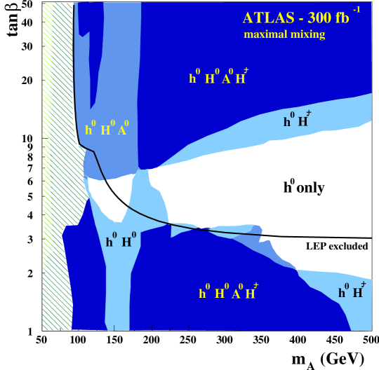
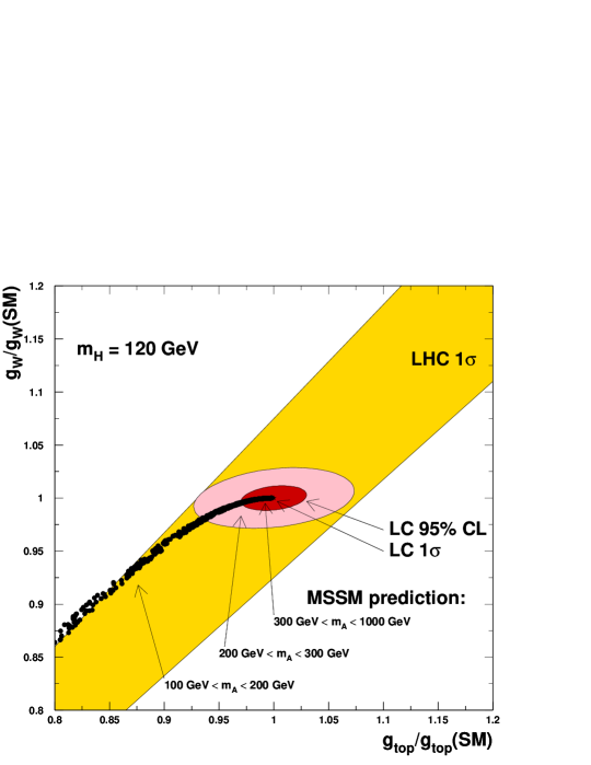
It is very clear that the precise and absolute measurement of all relevant Higgs boson couplings can only be performed at TESLA. Furthermore, the unambiguous determination of the quantum numbers of the Higgs boson and the high sensitivity to –violation represent a crucial test. The measurement of the Higgs self coupling gives access to the shape of the Higgs potential. These measurements together will allow to establish the Higgs meachnism as the mechanism of electroweak symmetry breaking.
At TESLA, extended Higgs sectors as present in supersymmetric thoeries can be distinguished from the SM Higgs sector with little assumptions about their precise structure. As an example, in the MSSM the boson can be distingished from SM Higgs boson over the whole parameter region shown in Fig. 1. Heavy Higgs bosons can studied if kinematically accessible with high precision.
Almost any conceivable extended Higgs boson scenario can be seen at TESLA. In particular any Higgs boson, which couples to the boson can be observed in production through the recoil mass method, independent of its decay. Therefore, TESLA is able to close possible loopholes, if they exist in the LHC discovery potential (e.g. the accessibility of invisibly decaying Higgs bosons was not confirmed so far by the LHC collaborations).
In summary, TESLA has the unique opportunity to study Higgs bosons with high precision in all essential aspects. These measurements will provide the information necessary to reveal the mechanism of electroweak symmetry breaking and mass generation.
| (GeV) | LHC | LC | |
| 2 300 fb-1 | 500 fb-1 | ||
| 120 | 9 | 3 | |
| 160 | 10 | 4 | |
| 120-140 | - | 0.04 - 0.06 | |
| 120-140 | - | 0.02 - 0.04 | |
| 120-140 | - | 0.01 - 0.02 | |
| 120-140 | - | 0.01 - 0.03 | |
| 120-140 | - | 0.023-0.052 | |
| 120-140 | - | 0.012-0.022 | |
| 120 | 0.070 | 0.023 | |
| 160 | 0.050 | 0.022 | |
| test | 120 | - | 0.03 |
| 120 | - | 0.22 |
References
- [1]
-
[2]
P.W. Higgs. Phys. Lett. 12:132, 1964;
P.W. Higgs. Phys. Rev. Lett. 13:508, 1964;
P.W. Higgs. Phys. Rev. 145:1156, 1966;
F. Englert, R. Brout. Phys. Rev. Lett. 13:321, 1964;
G.S. Guralnik, C.R. Hagen, T.W. Kibble. Phys. Rev. Lett. 13:585, 1964. - [3] For a review of the SM and MSSM Higgs sectors, see: J. Gunion, H.E. Haber, G. Kane, S. Dawson. The Higgs Hunter’s Guide. Addison Wesley, ISBN 0-7382-0305-X.
-
[4]
S.L. Glashow. Nucl. Phys. 20:579, 1961;
A. Salam, in Elementary Particle Theory, ed. N. Svartholm, 1968;
S. Weinberg. Phys. Rev. Lett. 19:1264, 1967;
G. ’t Hooft, M. Veltman. Nucl. Phys. B44:189, 1972. - [5] For a review on Supersymmetry, see J. Wess and J. Bagger. Supersymmetry and Supergravity. Princeton Series in Physics.
-
[6]
For reviews on the MSSM, see: P. Fayet and S. Ferrara.
Phys. Rept. 32:249, 1977;
H.P. Nilles. Phys. Rept. 110:1, 1984;
R. Barbieri. Riv. Nuovo Cim. 11:1, 1988;
H.E. Haber, G. Kane. Phys. Rept. 117:75, 1985. -
[7]
Some work described here has been worked out
in a series of workshops and reported in:
Collisions at 500 GeV: The Physics Potential.
Munich–Annecy–Hamburg 1991/93, DESY 92-123A+B, 93-123C;
Collisions at TeV Energies: The Physics Potential,
Annecy–Gran Sasso–Hamburg 1995, DESY 96-123D;
E. Accomando et al. Phys. Rept. 299:1, 1998. - [8] T. Hambye, K. Riesselmann. Phys. Rev. D55:7255, 1997.
- [9] The LEP Collaborations. A Combination of Preliminary Electroweak Measurements and Constraints on the Standard Model. CERN-EP Note in preparation.
- [10] B.W. Lee, C. Quigg, H.B. Thacker. Phys. Rev. 16:1519, 1977.
-
[11]
N. Cabibbo, L. Maiani, G. Parisi, R. Petronzio. Nucl. Phys. B158:295, 1979;
M. Sher. Phys. Rept. 179:273, 1989;
M. Lindner. Z. Phys. C31:295, 1986;
G. Altarelli, G. Isidori. Phys. Lett. B337:141, 1994;
J. Casas, J. Espinosa, M. Quiros. Phys. Lett. B342:171, 1995. -
[12]
A. Hasenfratz, K. Jansen, C.B. Lang, T. Neuhaus, H. Yoneyama.
Phys. Lett. B199:531, 1987;
M. Lüscher, P. Weisz. Phys. Lett. B212:472, 1988;
M. Göckeler, H.A. Kastrup, T. Neuhaus, F. Zimmermann. Nucl. Phys. B404:517, 1993. -
[13]
G. Altarelli, G. Isidori. Phys. Lett. B337:141, 1994;
J. Casas, J. Espinosa, M. Quiros. Phys. Lett. B342:171, 1995. - [14] Z.G. Zhao (BES Coll.). New Values in 2-5 GeV from the BESII at BEPC. To appear in the proceedings of the 30th Int. Conf. on High Energy Physics, 7 Jul - 2 Aug 2000, Osaka, Japan and hep-ex/0012038.
- [15] M. Davier, A. Höcker. Phys. Lett. B419:419, 1998.
- [16] V. A. Novikov, L. B. Okun, A. N. Rozanov and M. I. Vysotsky, Rept. Prog. Phys. 62:1275, 1999.
- [17] R. Barbieri, A. Strumia. Phys. Lett. B462:144, 1999.
-
[18]
P. Igo-Kemenes for the LEP working groups on Higgs boson
searches, Talk at the LEPC open session, November 3;
ALEPH Collaboration (R. Barate et al.). Phys. Lett. B495:1, 2000;
L3 Collaboration (M. Acciarri et al.). Phys. Lett. B495:18, 2000. -
[19]
J. Ellis, M.K. Gaillard, D.V. Nanopoulos. Nucl. Phys. B106:292, 1976;
B.L. Ioffe, V.A. Khoze. Sov. J. Nucl. Phys. 9:50, 1978;
B.W. Lee, C. Quigg, H.B. Thacker. Phys. Rev. 16:1519, 1977. -
[20]
D.R.T. Jones, S. Petcov. Phys. Lett. B84:440, 1979;
R. Cahn, S. Dawson. Phys. Lett. B136:196, 1984;
G. Kane, W. Repko, W. Rolnick. Phys. Lett. B148:367, 1984;
G. Altarelli, B. Mele, F. Pitolli. Nucl. Phys. B287:205, 1987;
W. Kilian, M. Krämer, P.M. Zerwas. Phys. Lett. B373:135, 1996. -
[21]
J.F. Gunion, H.E. Haber. Phys. Rev. D48:5109, 1993;
D.L. Borden, D.A. Bauer, D.O. Caldwell. Phys. Rev. D48:4018, 1993;
M. Baillargeon, G. Bélanger, F. Boudjema. Phys. Rev. D51:4712, 1995;
I.F. Ginzburg, I.P. Ivanov. Phys. Lett. B408:325, 1997;
A. Djouadi, V. Driesen, W. Hollik, J.I. Illana. Eur. Phys. J. C1:149, 1998. -
[22]
V.S. Fadin, V.A. Khoze, A.D. Martin. Phys. Rev. D56:484, 1997;
M. Melles, W.J. Stirling. Nucl. Phys. B564:325, 1999;
M. Melles, W.J. Stirling. Eur. Phys. J. C9:101, 1999. -
[23]
G. Jikia, S. Söldner-Rembold. Nucl. Phys. (Proc. Suppl.)
82:373, 2000;
G. Jikia, S. Söldner-Rembold. LC-PHSM-2001-060. -
[24]
A. Djouadi, M. Spira, P.M. Zerwas. Z. Phys. C70:427, 1996;
A. Djouadi, J. Kalinowski, M. Spira. Comp. Phys. Comm. 108:56, 1998. - [25] J. Wess, B. Zumino. Nucl. Phys. B70:39, 1974.
-
[26]
J.F. Gunion, H. Haber. Nucl.Phys. B272:1,1986,
Erratum-ibid. B402:567, 1993;
J.F. Gunion, H. Haber. Nucl. Phys. B279:449, 1986. -
[27]
Y. Okada, M. Yamaguchi, T. Yanagida. Prog. Theor. Phys. 85:1, 1991;
H.E. Haber, R. Hempfling. Phys. Rev. Lett. 66:1815, 1991;
J. Ellis, G. Ridolfi, F. Zwirner. Phys. Lett. B257:83, 1991;
R. Barbieri, F. Caravaglios, M. Frigeni. Phys. Lett. B258:167, 1991. -
[28]
M. Carena, J.R. Espinosa, M. Quiros, C.E.M. Wagner.
Phys. Lett. B355:209, 1995;
H.E. Haber, R. Hempfling, A. Hoang. Z. Phys. C75:539, 1997;
M. Carena, H.E. Haber, S. Heinemeyer, W. Hollik, C.E.M. Wagner, G. Weiglein. Nucl. Phys. B580:29, 2000. -
[29]
S. Heinemeyer, W. Hollik, G. Weiglein.Phys. Rev. D58:091701, 1998;
S. Heinemeyer, W. Hollik, G. Weiglein. Phys. Lett. B440:296, 1998. - [30] S. Heinemeyer, W. Hollik, G. Weiglein. Comp. Phys. Comm. 124:76, 2000.
- [31] H.E. Haber. Challenges for Nonminimal Higgs Searches at Future Colliders. 4th International Conference On Physics Beyond The Standard Model 13-18 Dec 1994, Lake Tahoe, California. CERN-TH-95-109, SCIPP-95-15.
-
[32]
J.F. Gunion, L. Roszkowski, A. Turski, H.E. Haber, G. Gamberini,
B. Kayser, S.F. Novaes. Phys. Rev. D38:3444, 1988;
A. Djouadi, J. Kalinowski, P.M. Zerwas. Z. Phys. C57:569, 1993;
A. Djouadi, J. Kalinowski, P. Ohmann, P.M. Zerwas. Z. Phys. C74:93, 1997;
S. Heinemeyer, W. Hollik, J. Rosiek and G. Weiglein. LC-TH-2001-037; http://www.desy.de/~lcnotes/. -
[33]
J.I. Illana. LC-TH-2000-002;
http://www.desy.de/~lcnotes/;
M. Mühlleitner, M. Kramer, M. Spira, P.M. Zerwas. Production of MSSM Higgs Bosons in Photon-Photon Collisions. DESY-00-192 and hep-ph/0101083. - [34] For an overview of Higgs boson decays in the MSSM, see for instance: A. Djouadi, J. Kalinowski, P.M. Zerwas. Z. Phys. C70:435, 1996.
-
[35]
H. Baer, D. Dicus, M. Drees, X. Tata. Phys. Rev. D36:1363, 1987;
K. Griest, H.E. Haber. Phys. Rev. D37:719, 1988;
J.F. Gunion, H.E. Haber. Nucl. Phys. B307:445, 1988, Erratum-ibid. B402:569, 1993;
A. Djouadi, P. Janot, J. Kalinowski, P.M. Zerwas. Phys. Lett. B376:220, 1996;
A. Djouadi, J. Kalinowski, P. Ohmann, P.M. Zerwas. Z. Phys. C74:93, 1997;
A. Bartl, H. Eberl, K. Hidaka, T. Kon, W. Majerotto, Y. Yamada. Phys. Lett. B389:538, 1996. - [36] A. Djouadi. Mod. Phys. Lett. A14:359, 1999.
-
[37]
P. Fayet. Nucl. Phys. B90:104, 1975;
H.-P. Nilles, M. Srednicki, D. Wyler. Phys. Lett. B120:346, 1983;
J.-P. Derendinger, C.A. Savoy. Nucl. Phys. B237:307, 1984;
J.F. Gunion, H.E. Haber. Nucl. Phys. B272:1, 1986, Erratum-ibid.B402:567, 1993; part 1
part 2
J. Ellis, J.F. Gunion, H.E. Haber, L. Roszkowski, F. Zwirner. Phys. Rev. D39:844, 1989. -
[38]
U. Ellwanger, M. Rausch de Traubenberg, C.A. Savoy.
Z. Phys. C67:665, 1995;
S.F. King, P.L. White. Phys. Rev. D52:4183, 1995;
H. Asatrian, K. Egiin. Mod. Phys. Lett. A10:2943, 1995. . -
[39]
J.R. Espinosa, M. Quiros. Phys. Lett. B279:92, 1992;
G.L. Kane, C. Kolda, J.D. Wells. Phys. Rev. Lett. 70:2686, 1993;
J. Kamoshita, Y. Okada, M. Tanaka. Phys. Lett. B328:67, 1994. - [40] J.R. Espinosa, M. Quiros. Phys. Rev. Lett. 81:516, 1998.
- [41] J. R. Espinosa, J. F. Gunion. Phys. Rev. Lett. 82:1084, 1999.
- [42] P. Garcia-Abia and W. Lohmann. EPJdirect C2:1, 2000, LC-PHSM-2000-063; http://www.desy.de/~lcnotes/.
- [43] P.Garcia-Abia, W. Lohmann, A. Raspereza. LC-PHSM-2000-062; http://www.desy.de/~lcnotes/.
- [44] J.-C. Brient. LC-PHSM-2000-049; electronic document http://www.desy.de/~lcnotes/.
- [45] M. Battaglia, D. Schulte. LC-PHSM-2000-052; http://www.desy.de/~lcnotes/.
- [46] K. Desch, N. Meyer, LC-PHSM-2001-025; electronic document http://www.desy.de/~lcnotes/.
- [47] G. Moortgat–Pick, H. Steiner. LC-TH-2000-055; http://www.desy.de/~lcnotes/.
- [48] G. Borisov, F. Richard. Precise Measurement of Higgs Decay Rate into at future Linear Colliders and theoretical Consequences. LAL 99-26, hep-ph/9905413.
-
[49]
E. Boos,V. Ilyin, A. Pukhov, M. Sachwitz, H.J. Schreiber.
EPJdirect C5:1, 2000;
E. Boos,V. Ilyin, A. Pukhov, M. Sachwitz, H.J. Schreiber. LC-PHSM-2000-035; http://www.desy.de/~lcnotes/. - [50] M. Melles, W.J. Stirling, V.A. Khoze. Phys. Rev. D61:54015, 2000.
- [51] E. Boos, J.C. Brient, D.W. Reid, H.J. Schreiber, R. Shanidze. DESY-00-162, LC-PHSM-2000-053; http://www.desy.de/~lcnotes/.
- [52] M.D. Hildreth, T.L. Barklow, D.L. Burke. Phys. Rev. D49:3441, 1994.
- [53] M. Battaglia, in Proc. of the Worldwide Study on Physics and Experiments with Future Linear Colliders, E. Fernandez and A. Pacheco (editors), UAB, Barcelona 2000, vol. I, 163 and M. Battaglia, to appear in Eur. Phys. J..
-
[54]
A. Djouadi, J. Kalinowski, P.M. Zerwas. Mod. Phys. Lett. A7:1765, 1992;
A. Djouadi, J. Kalinowski, P.M. Zerwas. Z. Phys. C54:255, 1992. -
[55]
S. Dittmaier, M. Kramer, Y. Liao, M. Spira, P.M. Zerwas.
Phys. Lett. B441:383, 1998;
S. Dittmaier, M. Kramer, Y. Liao, M. Spira, P.M. Zerwas. Phys. Lett. B478:247, 2000;
S. Dawson, L. Reina. Phys. Rev. D57:5851, 1998;
S. Dawson, L. Reina. Phys. Rev. D59:054012, 1999. -
[56]
A. Juste, G. Merino. Top-Higgs Yukawa Coupling Measurement at a Linear
Collider. hep-ph/9910301;
H. Baer, S. Dawson, L. Reina. Phys. Rev. D61:013002, 2000. - [57] J. Alcaraz, E.R. Morales. Measuring the Top Yukawa Coupling to a heavy Higgs Boson at future Linear Colliders. To appear in the Proc. of the Int. Workshop on Linear Colliders - LCWS2000, Fermilab, October 2000. hep-ph/0012109.
- [58] K. Desch, M. Battaglia, to appear in the Proc. of the Int. Workshop on Linear Colliders - LCWS2000, Fermilab, October 2000, LC-PHSM-2001-053; http://www.desy.de/~lcnotes/.
-
[59]
V. Barger, K. Cheung , A. Djouadi, B.A. Kniehl, P.M. Zerwas .
Phys. Rev. D49:79, 1994;
K. Hagiwara, M.L. Stong. Z. Phys. C62:99, 1994. - [60] D.J. Miller, S.Y. Choi, B. Eberle, M.M. Muhlleitner,P.M. Zerwas. LC-TH-2001-033; http://www.desy.de/~lcnotes/.
- [61] M.T. Dova, P. Garcia-Abia, W. Lohmann. LC-PHSM-2001-054; http://www.desy.de/~lcnotes/.
- [62] A. Djouadi, B.A. Kniehl. Correlations in Higgs Production and Decay as a Probe of CP Violation in the Scalar Sector. DESY 93-123C, p. 51.
-
[63]
D. Atwood, A. Soni. Phys. Rev. D45:2405, 1992;
M. Davier, L. Duflot, F. Le Diberder, A. Rouge. Phys. Lett. B306:411, 1993;
M. Diehl, O. Nachtmann. Z. Phys. C62:397, 1994. - [64] M. Schumacher. LC-PHSM-2001-003; http://www.desy.de/~lcnotes/.
- [65] K. Hagiwara, S. Ishihara, J. Kamoshita, B.A. Kniehl. Eur. Phys. J. C14:457, 2000.
- [66] J.F. Gunion, B. Grzadkowski, X.-G. He. Phys. Rev. Lett. 77:5172, 1996.
- [67] G. Gounaris, D. Schildknecht, F.M. Renard. Phys. Lett. B83:191, 1979.
- [68] A. Djouadi, W. Kilian, M. Mühlleitner, P.M. Zerwas. Eur. Phys. J. C10:27, 1999.
- [69] D.J. Miller, S. Moretti. Eur. Phys. J. C13:459, 2000.
- [70] C. Castanier, P. Gay, P. Lutz, J. Orloff. LC-PHSM-2000-061; http://www.desy.de/~lcnotes/.
- [71] J. Guasch, W. Hollik, A. Kraft. LC-TH-1999-006 and hep-ph/9911452; http://www.desy.de/~lcnotes/.
- [72] A. Kiiskinen, M. Battaglia, P. Pöyhönen. Study of at a 800 GeV Linear Collider. To appear in the Proc. of the Int. Workshop on Linear Colliders - LCWS2000, Fermilab, October 2000, LC-PHSM-2001-041; ; http://www.desy.de/~lcnotes/.
- [73] A. Andreazza, C. Troncon. Study of HA Production in Collisions at =800 GeV. DESY-123-E, p. 417.
- [74] J. Kamoshita, Y. Okada, M. Tanaka, in Proc. of the Workshop on Physics and Experiments with Linear Colliders, A. Miyamoto et al. (editors), World Scientific 1996.
-
[75]
L.J. Hall, R. Rattazzi, U. Sarid.
Phys. Rev. D50:7084, 1994;
M. Carena, S. Mrenna, C.E.M Wagner. Phys. Rev. D60:075010, 1999;
M. Carena, S. Mrenna, C.E.M Wagner. Phys. Rev. D62:055008, 2000;
H. Eberl, K. Hidaka, S. Kraml, W. Majerotto, Y. Yamada. Phys. Rev. D62:055006, 2000;
M. Carena, D. Garcia, U. Nierste, C.E.M. Wagner. Nucl. Phys. B577:88, 2000. - [76] M. Berggren, R. Keranen, A. Sopczak. EPJdirect C8:1, 2000.
- [77] S. Kanemura, T. Kasai, Y. Okada. Phys. Lett. B471:182, 1999.
-
[78]
J.F. Gunion, L. Poggioli, R. Van Kooten, C. Kao, P. Rowson. Higgs
Boson Discovery and Properties. hep-ph/9703330 ;
M. Krawczyk, to appear in the Proc. of the Int. Workshop on Linear Colliders, Fermilab, October 2000;
I. F. Ginzburg, M. Krawczyk and P. Osland. Distinguishing Higgs Models at Photon Colliders. hep-ph/9909455. -
[79]
P. Chankowski, T. Farris, B. Grzadkowski, J.F. Gunion,
J. Kalinowski, M. Krawczyk. Phys. Lett. B496:195, 2000;
P.H. Chankowski, M. Krawczyk, J. Zochowski. Eur. Phys. J. C11:661, 1999. - [80] For the one-loop couplings see J. F. Gunion, H.E. Haber, C. Kao. Phys. Rev. D46:297, 1992.
-
[81]
J.F. Gunion, B. Grzadkowski, H.E. Haber, J. Kalinowski.
Phys. Rev. Lett. 79:982, 1997;
B. Grzadkowski, J. F. Gunion, J. Kalinowski. Phys. Rev. Lett. 60:075011, 1999;
B. Grzadkowski, J. F. Gunion, J. Kalinowski. Phys. Lett. B480:287, 2000. - [82] M. Krawczyk, J. Zochowski, P. Mattig. hep-ph/0009201 M. Krawczyk, J. Zochowski, P. Mattig. Eur. Phys. J. C8:495, 1999.
-
[83]
J. F. Gunion, L. Roszkowski, A. Turski. Phys. Rev. D38:3444, 1988;
H.E. Haber, Y. Nir. Phys. Lett. B306:327, 1993;
A. Djouadi, H.E. Haber, P.M. Zerwas. Phys. Lett. B375:203, 1996. -
[84]
T. Binoth, J.J. van der Bij. Z. Phys. C75:17, 1997;
T. Binoth, J.J. van der Bij. Proc. of the Worldwide Study on Physics and Experiments with Future Linear Colliders. E. Fernandez and A. Pacheco (editors), UAB, Barcelona 2000, Vol. I, 591 and hep-ph/9908256. - [85] ATLAS Collaboration. ATLAS Detector and Physics Performance Technical Design Report. CERN-LHCC 99-14.
- [86] CMS Collaboration. CMS Technical Proposal. CERN-LHCC 94-38.
- [87] D. Zeppenfeld, R. Kinnunen, A. Nikitenko, E. Richter-Was. Phys. Rev. D62:13009, 2000.
- [88] V. Drollinger, A. Sopczak. LC-PHSM-2000-037; http://www.desy.de/~lcnotes/.
Chapter 2 Supersymmetry
Despite the enormous success of the Standard Model (SM) this cannot be the ultimate wisdom to understand nature for many reasons. The introduction of Supersymmetry (SUSY) is considered the most attractive extension of the Standard Model [1]. Firstly, there are important theoretical motivations. It is the only non–trivial extension of the Poincaré group in quantum field theory. SUSY as a local symmetry becomes a supergravity (SUGRA) theory, incorporating gravity. SUSY appears in superstring theories, which may lead to the final theory of all fundamental interactions. From a phenomenological point of view, the most important feature of SUSY is that it can explain the hierarchy between the electroweak scale of 100 GeV, responsible for the and masses, and the unification scale GeV or the Planck scale GeV. It also stabilises the Higgs mass with respect to radiative corrections, if TeV. Moreover, the Minimal Supersymmetric Standard Model (MSSM) allows the unification of the gauge couplings of electroweak and strong interactions and yields precisely the measured value of . Furthermore, in the MSSM electroweak symmetry breaking is a natural result of renormalisation group evolution. Another attractive feature of SUSY is that the lightest supersymmetric particle is a good cold dark matter candidate. Furthermore, a supersymmetric theory naturally contains extra sources of CP violation to ensure baryogenesis assuming an initially matter–antimatter symmetric universe.
Most motivations for supersymmetry lead us to expect that SUSY particles will be found at the next increase in energy, at Tevatron and/or LHC. If gluinos and squarks have masses below TeV, they will be seen at LHC. In most scenarios some SUSY particles, especially the partners of and , the charginos and neutralinos, are expected to be lighter and should lie in the energy region of Tesla. Examples of mass spectra for three SUSY breaking mechanisms are shown in Fig. 1.
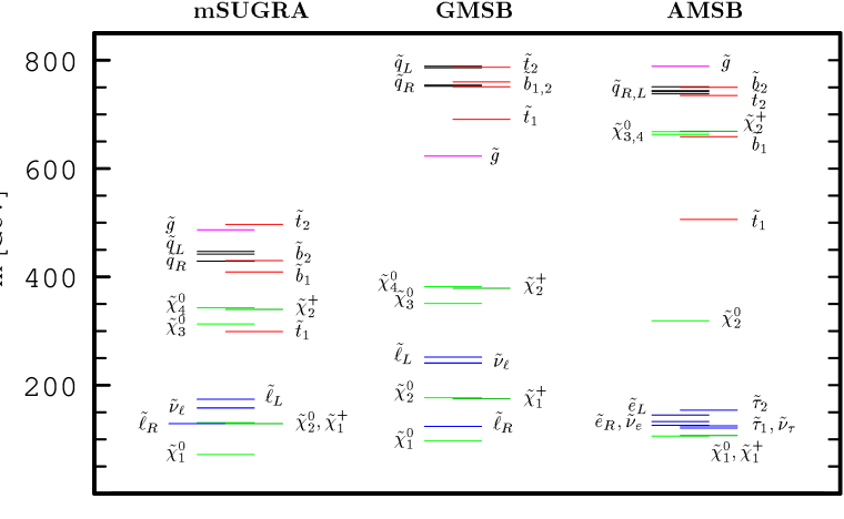
The discovery potential of Tesla for SUSY particles has been extensively studied in the literature and in previous workshops [2]. Two important new issues have been addressed at the 2nd Joint ECFA/DESY Study [3]: The availability of high luminosity, per year, and of polarised electron and positron beams. The high luminosity makes precision experiments possible. We will therefore discuss in detail accurate measurements of the masses of SUSY particles and the determination of the couplings and mixing properties of sleptons, charginos, neutralinos and scalar top quarks. A precise knowledge of the sparticle spectrum and the SUSY parameters is necessary to reveal the underlying supersymmetric theory.
If kinematically accessible the complete sparticle spectrum can be studied in detail with the high luminosity available at Tesla. It is vital to have highly polarised electrons and it is very desirable to have polarised positrons as well. It is assumed that polarisations of for electrons and for positrons are achievable. A proper choice of polarisations and center of mass energy helps disentangle the various production channels and suppress background reactions. Electron polarisation is essential to determine the weak quantum numbers, couplings and mixings. Positron polarisation provides additional important information [4]: (i) an improved precision on parameter measurements by exploiting all combinations of polarisation; (ii) an increased event rate (factor 1.5 or more) resulting in a higher sensitivity to rare decays and subtle effects; and (iii) discovery of new physics, e.g. spin 0 sparticle exchange. In general the expected background is dominated by decays of other supersymmetric particles, while the Standard Model processes like production can be kept under control at reasonably low level.
The most fundamental open question in SUSY is how supersymmetry is broken and in which way this breaking is communicated to the particles. Here three different schemes are considered: the minimal supergravity (mSUGRA) model, gauge mediated (GMSB) and anomaly mediated (AMSB) supersymmetry breaking models. The phenomenological implications are worked out in detail. The measurements of the sparticle properties, like masses, mixings, couplings, spin-parity and other quantum numbers, do not depend on the model chosen.
In a kind of ‘bottom–up’ approach a study demonstrates how the SUSY parameters, determined at the electroweak scale with certain errors, can be extrapolated to higher energies. In this way model assumptions made at higher energies, for example at the GUT scale, can be tested.
–parity conservation is an additional assumption in most SUSY models. However, there is no fundamental reason for this, and a section is devoted to the phenomenology of –parity violation.
Finally, a comparison is made between Tesla and LHC concerning the determination of the SUSY particle spectrum and the SUSY parameters.
1 The Minimal Supersymmetric Standard Model
The Minimal Supersymmetric Standard Model (MSSM) is the minimal extension of the Standard Model (SM) to incorporate supersymmetry [1]. In addition to the particles of the SM, the MSSM contains their supersymmetric partners: sleptons , (), squarks and gauginos . Two Higgs doublets are necessary: ) and , together with their superpartners, the higgsinos (). The two doublets lead to five physical Higgs bosons (, .
The non–strongly interacting gauginos mix with the higgsinos to form corresponding mass eigenstates: two pairs of charginos and four neutralinos . The masses and couplings of the charginos and neutralinos are determined by the corresponding mass matrices, which depend on the parameters and . Usually, the GUT relation is taken.
Corresponding to the two chirality states of the leptons and quarks one has the left and right scalar partners , and . In the third generation one expects mixing between the and states with mass eigenstates called and .
In the MSSM the multiplicative quantum number –parity is conserved, for SM particles and for the supersymmetric partners. This implies that there is a lightest supersymmetric particle (LSP), which is stable and into which all SUSY particles eventually decay. Usually, the neutralino is assumed to be the LSP.
In the most general case, the MSSM contains 105 parameters in addition to the SM parameters. This number can be considerably reduced by invoking specific models, which allow a systematic study of the whole parameter space. In the so–called minimal supergravity (mSUGRA) model, due to universal unification conditions at GeV, one has only five parameters , , , and , where and are the common scalar mass and gaugino mass at and is the universal trilinear coupling parameter.
In the following studies two mSUGRA scenarios, labeled RR1 and RR2, are used to calculate masses, cross sections, branching ratios and other physical quantities [3]. The model parameters for RR1 are: GeV, GeV, GeV, , ; the corresponding mass spectrum is shown in Fig. 1. The parameters for RR2 are: GeV, GeV, GeV, , . The low scenario gives a Higgs mass of GeV, which is ruled out by LEP searches. The mass does not affect the studies discussed here, it only enters in cascade decays of the higher states. Moreover, a Higgs mass of, for instance, 115 GeV can be achieved within mSUGRA by shifting the trilinear coupling GeV and , which has only little influence on the slepton, chargino and neutralino masses and properties.
2 Sleptons
Scalar leptons are the superpartners of the right-handed and left-handed leptons. They are produced in pairs
| (1) | |||||
via -channel exchange. In addition the -channel contributes in selectron production via neutralinos and in electron-sneutrino production via charginos. The two-body kinematics of the decays and allows a clean identification and accurate measurements of the sparticle masses involved and other slepton properties like spin, branching ratios, couplings and mixing parameters. Polarisation is indispensible to determine the weak quantum numbers of the sleptons. Detailed simulations of slepton production based on the Tesla detector design are reported by [5, 6], where it is assumed that beam polarisations of and are available.
1 Mass determinations
The potential of an collider will be illustrated for the second generation of sleptons and . The simplest case is the production and decay of right smuons . The results of a simulation are shown in Fig. 1 a. The dominant background from production can be kept small. The energy spectrum of the decay muons is flat apart from beamstrahlung, initial state radiation and resolution effects at the high edge. The end points can be related to the masses and of the primary and secondary particles with an accuracy of about 3 per mil. If the neutralino mass can be fixed by other measurements one can exploit the momentum correlations of the two observed muons [7] and construct the minimum kinematically allowed smuon mass . From the ‘end point’ or maximum of this distribution, shown in Fig. 1 b, the accuracy on can be improved by a factor of two.
Higher accuracy can be achieved by measuring the pair production cross section around threshold, which rises as , see Fig. 1c. For an integrated luminosity of , to be collected within a few month at Tesla, a mass resolution GeV can be reached. With such a sensitivity finite width effects cannot be neglected [6]. From a fit to the excitation curve one expects to measure the width, here GeV, with an error of the same order. It is also important to include in the threshold cross section calculations sub-dominant diagrams which lead to the same final state, because they may mimic a mass shift comparable to the resolution [8].
The left partner is more difficult to detect due to background from pairs and SUSY cascade decays. It can be identified via a unique signature: followed by . Despite the low cross section, fb in scenario RR1, such a measurement is feasible at Tesla, see Fig. 2 a, providing the masses and with a precision of 2 per mil. Another example is sneutrino production, where the flavour is tagged via its charged decay . The subsequent decays and lead to a clean topology. The spectrum of the primary muons in Fig. 2 can be used to determine and to better than 2 per mil.
Even more accurate mass measurements can be done for the first generation of sleptons and , due to much larger cross sections from additional -channel contributions. Of particular interest is associated selectron production via exchange.The cross section rises as , contrary to other slepton pairs, which is an advantage for mass determination via threshold scans. In case of polarised beams the charge of the observed lepton can be directly related to the quantum number of the produced selectron, and . This elegant separation of the selectron decay spectra can be considerably improved if not only the beam but also the beam is polarised.
Assuming that the incoming electrons and positrons have the same helicity only the –channel production and is possible. This allows one to easily identify and separately.
132.0 0.3 0.09 176.0 0.3 0.4 160.6 0.2 0.8 132.0 0.2 0.05 176.0 0.2 0.18 160.6 0.1 0.07 131.0 0.6 177.0 0.6 160.6 0.6 127.7 0.2 0.04 345.8 0.25 71.9 0.1 0.05 130.3 0.3 0.07 319.8 0.30 348.2 0.52
Measurements of and of the third slepton generation are less favourable. While identification via decays will be easy and efficient, the background is large ( production) and a mass determination via energy spectra is much less accurate, of the order of a few per cent [9]. But from cross section measurements at threshold one may obtain mass resolutions around half a per cent. The expected accuracies on slepton masses for mSUGRA model RR1 are given in Table 1.
2 Slepton properties
A very important topic is the determination of the quantum numbers. Sleptons carry spin 0, but otherwise the SM quantum numbers of leptons. The differential cross section for -channel exchange is proportional to . A consistency check, although not unique, can be obtained from the dependence of the cross section scan at threshold. A more direct method is to measure the angular distribution of the sleptons. Using the masses of the particles involved the event kinematics allows the slepton directions to be reconstructed up to a twofold ambiguity. The wrong solution turns out to be flat in and can be subtracted. The smuon angular distribution for production is displayed in Fig. 3 and clearly exhibits the expected behaviour of a scalar spin 0 particle. The association of and to their right-handed and left-handed SM partners can be unambiguously done by studying the dependence of the production cross section on the electron and/or positron beam polarisation.

Precise mass measurements allow the flavour dependence of the underlying supersymmetry model to be checked at the level of one per mil for the first two slepton generations and to a few per mil for the stau family. An important application is to test general SUSY mass relations. The tree level prediction
| (2) |
offers a model independent determination of from the slepton sector. Using typical measurements as given in Table 1 one finds . The sensitivity degrades at larger values to .
In the case of large the slepton analyses of the first and second generation remain essentially unaffected. Major differences occur in the stau sector where a large mass splitting between and is expected. The physical eigenstates are mixed, and , and are no longer degenerate with the selectron and smuon masses. These properties allow to be accessed via the relation
| (3) |
which follows from the diagonalisation of the mass matrix. If the directly measurable quantities and can be determined to and to (from the chargino sector), one can extract with an accuracy of , dominated by large uncertainties on the value of .
It has been noted that the polarisation of tau’s in the decay is very sensitive to if it is large or if has a large higgsino component [9]. The measurement is based on the characteristic energy distributions of the decay products of the polarised . In a combined analysis of and pair production for , one obtains an accuracy of , depending slightly on the gaugino parameter .
3 Charginos and Neutralinos
Charginos and neutralinos are produced in pairs
| (1) | |||||
| (2) |
via -channel exchange and -channel selectron or sneutrino exchange. They are easy to detect via their decays into lighter charginos/neutralinos and gauge or Higgs bosons or into sfermion-fermion pairs. If these two-body decays are kinematically not possible, typically for the lighter chargino and neutralino, they decay via virtual gauge bosons and sfermions, e.g. or . In -parity conserving MSSM scenarios the lightest neutralino is stable.The experimental signatures are multi-lepton and/or multi-jet events with large missing energy. Detailed Tesla detector simulations of chargino and neutralino production assuming beam polarisations of and are performed in [5].
1 Mass determinations
The lightest observable neutralino can be detected via its 3-body decay . In direct production the energy spectra of the di-lepton systems, Fig. 1, can be used to determine the masses of the primary and secondary neutralinos with typical uncertainties of 2 per mil. From the di-lepton mass spectrum one gets additional information on the mass difference . Moreover, ’s are abundantly produced in decay chains of other SUSY particles. By exploiting all di-lepton modes it will be possible to measure the mass difference with a precision of better than MeV, limited only by the resolution of the detector.
Charginos will be copiously produced, for example , see Fig. 2. Using the same techniques as for neutralinos, the di-jet energy distribution gives an accuracy of GeV. Similarly, the di-jet mass spectrum allows to get the chargino-neutralino mass difference to better than MeV, when using all possible cascade decays.
The cross sections for neutralino and chargino pair production rise as . This leads to steep excitation curves around threshold, see Figs. 1 c and 2 c, from which excellent mass resolutions of with an integrated luminosity of can be obtained for the light chargino/neutralinos, degrading for the heavier states to the per mil level. At the same time, the shape of the cross section at threshold provides a consistency check of a spin assignment to neutralinos and charginos. The expected accuracies of various mass determinations are summarised in Table 1 for mSUGRA scenario RR1.
For large the chargino and neutralino decays may be very different. Depending on the SUSY parameters the mass splitting of the sector, which rises with , see eq. (3), may result in a situation where . As a consequence the chargino decay and the neutralino decay dominate over all other decay modes via lepton or quark pairs. Although ’s are easy to detect, their energy cannot be reconstructed (missing neutrinos) and their decay products provide much less information on masses and mass differences of the states. A simulation of at GeV with GeV, GeV, GeV and is reported by [10]. Fitting the energy distribution of hadronic decays results in resolutions of about for the and masses. Note that chargino and neutralino cross section measurements, in particular around threshold, are much less affected by topologies and become more important for precise mass determinations in large scenarios.
2 Chargino properties
Charginos are composed of Winos and Higgsinos. An easy way to access the Wino component is via -channel exchange, which couples only to left-handed electrons. Thus the mixing parameters of the chargino system can be determined by varying the beam polarisation. Such studies have been presented in detail by [11, 12]. The chargino mass matrix in the basis
| (5) |
depends on the parameters , and . Two mixing angles and are needed to diagonalise the mass matrix. If the collider energy is sufficient to produce all chargino states of reaction (1) the underlying SUSY parameters can be extracted in a model independent way from the masses and production cross sections [11].
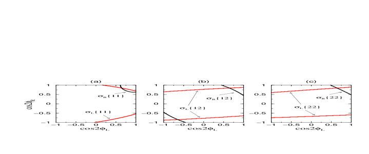
Figure 3 shows lines of constant cross sections for pair production with completely polarised electrons in the plane. Ambiguities can be resolved and the expected accuracy on the mixing angles is and for a total luminosity . Given precise measurements of and the exchanged sneutrino mass , the fundamental supersymmetry parameters , , and (low to medium) can be accurately determined independently of the structure of the neutralino sector, as illustrated in Table 1. If is large, this parameter is difficult to extract, only a significant lower bound can be derived. In this case the sector provides a higher sensitivity, see section 2.
| input RR1 | fit value | input RR2 | fit value | |
| 152 GeV | GeV | 150 GeV | GeV | |
| 316 GeV | GeV | 263 GeV | GeV | |
| 3 | 30 | |||
| 78.7 GeV | GeV | 78.0 GeV | GeV | |
The analysis of the chargino system depends via the cross sections on the mass of the exchanged sneutrino which may not be directly accessible, e.g. if . The sensitivity to the sneutrino mass can be considerably enhanced by a proper choice of polarisations and by making use of spin correlations between production and decay in the reaction and [12]. From the cross section and the forward-backward asymmetry of the decay electrons, shown in Fig. 4, one can determine sneutrino masses up to TeV with a precision of GeV.
For final precision measurements the inclusion of electroweak radiative corrections will be important, as they have been calculated for example in [13].
3 Neutralino properties
In a similar way the properties of the neutralino system, which is a mixture of Bino, Wino and two Higgsino fields, have been investigated. In a general MSSM model the neutralino sector depends in addition to , and on the gaugino parameter . Very useful analysis tools are angular distributions of leptons in the reaction exploiting spin correlations [14]. Figure 5 shows the sensitivity of the production cross section and the forward-backward asymmetry of the decay electron to the parameter . Again the importance of beam polarisations to determine the neutralino mixing parameters is clearly borne out.
A richer neutralino spectrum with quite different properties is expected if supersymmetry is extended by an additional Higgs superfield, like in the NMSSM or inspired models. With the high luminosity available at Tesla neutralinos with a dominant singlino component can be easily detected and studied over large regions in the parameter space [15]. A characteristic feature of these scenarios is that in certain parameter regions the second lightest supersymmetric particle may have a long life time leading to displaced vertices. Polarisation of both beams is important to enhance the production cross sections and to determine the underlying SUSY model [4].
Quite generally, the parameters , and can be complex, which also leads to violation. It is, however, possible to take real, so that only two phases remain, and . A method to extract from chargino production is described in [11] giving . A rather simple algebraic algorithm has been proposed by [16] to determine , , , , for given in terms of the masses of both charginos and two neutralinos and one of the chargino mixing angles as physical input. The remaining twofold ambiguity in and can be resolved by a measurement of the production cross section.
4 Stop Particles
Supersymmetry requires the existence of scalar partners and to each fermion . In case of the scalar partners of the top quark one expects a large mixing between and due to the large top quark mass thus making the lighter mass eigenstate presumably lighter than the squark states of the first two generations. In collisions stops can be pair produced by exchange
| (1) |
The cross sections have a very characteristic dependence on the stop mixing angle , where and .
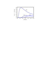
The phenomenology of stop production and decay at a linear collider has been discussed in detail in [17]. Figure 1 shows the energy dependence of the pair production cross sections. Initial state radiation, supersymmetric QCD [18, 19] and Yukawa coupling corrections [20] are included.
Figure 2 a shows the contour lines of the cross section as a function of the and beam polarisation. The cross section can be significantly increased by choosing the maximally possible and polarisation. Using polarised beams one can also measure the left–right polarisation asymmetry
| (2) |
where and . This observable is very sensitive to the stop mixing , as shown in Fig. 2 b.
1 Parameter determination
Owing to the large luminosity and the availability of polarised beams, it is possible to determine the mass and the mixing angle of the stop very precisely. One method consists of measuring production cross sections and of different polarisations.
A simulation of with decay modes and is performed in [21] including full SM background. The decay results in a signature of two jets and large missing energy, while leads to two jets, further jets from the decay and missing energy. The study, based on a fast simulation of the Tesla detector, is done for GeV and with GeV for the neutralino decay channel and GeV, GeV for the chargino channel. For 80% and 60% polarization and assuming , a measurement of the stop production cross section with a statistical error of 1.5% for and about 0.75% for appears feasible. The systematical error is of the order of 1%. Figure 3 a shows the corresponding , measurements in the plane. For the channel one obtains accuracies of GeV and . The errors for the decay are about half the size.
A more precise determination of the stop mass can be achieved by a method proposed in [7]. The mass is obtained as ‘end-point’ of the minimum kinematically allowed squark mass distribution (in analogy to the smuon case, Fig. 1b). Taking into account initial state radiation of photons and gluon radiation, a mass of GeV can be determined with a statistical error of with an integrated luminosity of [22].
A very good way to measure the stop mixing angle is to use the left–right asymmetry , eq. (2), where kinematic effects and uncertainties should largely cancel. For the parameter point above one gets an error on at the per mil level with an integrated luminosity of for each beam polarisation [17], cf. Fig. 2 b.
If the energy is high enough the heavier stop can also be produced via , and its mass can be determined. The stop masses , and the mixing are related to the basic soft SUSY breaking parameters and , which can be calculated if and are known. With measured to an error of and if and are known from other measurements to , then and can be determined with an accuracy of few percent [17].
Direct information on the stop parameters can be combined with indirect information by requiring consistency of the MSSM with precise measurements of the Higgs-boson mass , and the electroweak observables and [23]. This is shown in Fig. 3 b, where the allowed parameter space expected from future measurements at LHC and Tesla is displayed in the plane, for the stop parameters of Fig. 3 a and the other MSSM parameters chosen according to the RR2 scenario. The allowed region is significantly reduced by data from Tesla, in particular in the GigaZ scenario. Using from polarised cross section measurements one gets with a precision of . A comparison with direct mass measurements would test the MSSM at its quantum level in a sensitive and highly non-trivial way.
In general, the stop can decay in a variety of ways depending on its mass and those of the other SUSY particles [17]. There are additional two–body decays: , , , and . If these decays are kinematically not possible, the loop–decays [24] as well as three– [25] and four– [26] particle decays can be important.
One should point that a light stop of GeV may escape detection at the hadron colliders Tevatron and LHC and may only be discovered at Tesla.
5 The Minimal Supergravity (mSUGRA) Model
In supergravity supersymmetry is broken in a ‘hidden’ sector and the breaking is transmitted to the ‘visible’ sector by gravitational interactions. In the more specific minimal supergravity (mSUGRA) model all scalar particles (sfermions and Higgs bosons) have a common mass at the unification point GeV. The gaugino masses (corresponding to and , respectively) unify to a common gaugino mass and all trilinear coupling paramters have the same value at . One also has unification of the electroweak and strong coupling parameters . A further reduction of the parameters is given by invoking ‘radiative electroweak symmetry breaking’. As a consequence, one has only the following input parameters: . The whole SUSY particle spectrum can then be calculated by making use of renormalization group equations.
In mSUGRA it turns out quite generally that , so that . Both and are gaugino–like, is almost a pure –ino and is almost a pure –ino. The slepton masses of the first and second generation are given by: , , and . Analogous equations hold for squarks. It is also noteworthy that in mSUGRA the lightest neutralino is most naturally a good dark matter candidate if GeV [27].
The precise mass measurements of sleptons, neutralinos and charginos described in sections 2 and 3 (see Table 1) constitute an over–constrained set of observables which allow to determine the structure and parameters of the underlying SUSY theory [5]. A widely employed strategy, for example at the LHC, is to assume a SUSY breaking scenario and then fit to the corresponding low–energy particle spectrum including experimental uncertainties. Applying such a model dependent top–down approach to scenario RR1, one expects accuracies on the mSUGRA parameters as given in Table 1.
| parameter | input RR1 | error |
|---|---|---|
| 100 GeV | 0.09 GeV | |
| 200 GeV | 0.10 GeV | |
| 0 GeV | 6.3 GeV | |
| 3 | 0.02 | |
| + | no fit | |
The common scalar and gaugino masses and can be determined to better than one per mil, to better than a percent, and there is even some sensitivity to the trilinear coupling (coming from the higher mass sparticles). The magnitude of is obtained implicitly by the requirement of electroweak symmetry breaking.
While this method is a useful illustration of the SUSY measurement potential, the scenario assumptions are effectively constraints in the fit. This is particularly dangerous for models with pseudo-fixed point structures, where the low energy predictions will be quite similar for a large range of fundamental parameters. Also, new intermediate scales below the GUT scale will not be immediately apparent in a top–down approach. The advantages of Tesla to perform a model independent analysis of SUSY parameters will be discussed in section 10.
6 Gauge–Mediated SUSY Breaking (GMSB)
In supergravity models the typical fundamental scale of SUSY breaking is . An alternative possibility is that supersymmetry breaking occurs at lower energies with gauge interactions serving as the messengers, referred to as ‘gauge mediated supersymmetry breaking’ (GMSB) [28]. It avoids some potential problems of SUGRA, e.g. flavour changing neutral currents and CP violation. GMSB models are also very predictive as the MSSM spectrum depends on just a few parameters:
| (1) |
where is the messenger scale and is the messenger index parameterising the structure of the messenger sector. is the universal soft SUSY breaking scale felt by the low energy sector.
The MSSM parameters and the sparticle spectrum (at the weak scale) are determined from renormalisation group equation evolution starting from boundary conditions at the messenger scale . The gaugino masses at are given by and the squark/slepton masses by , where and are one– and two–loop functions and are known constants. If GeV at the electroweak scale, then TeV. As an illustration a GMSB sparticle mass spectrum is shown in Fig. 1. The charginos, neutralinos and sleptons are much lighter than the gluino and squarks.
A very interesting feature of GMSB is that the lightest supersymmetric particle is the gravitino
| (2) |
where GeV is the reduced Planck mass and is the fundamental scale of SUSY breaking with a typical value of TeV. Therefore, the phenomenology is strongly determined by the next-to-lightest SUSY particle (NLSP), which decays into the gravitino . The NLSP can be the neutralino, which decays dominantly via . The lifetime is given by
| (3) |
where is of order unity depending on the nature of the NLSP. Assuming keV as favoured by cosmology, typical decay lengths range from micro-meters to tens of meters. Figure 6 shows the neutralino NLSP lifetime as a function of the messenger scale and for various sets of GMSB parameters [29].
Figure 1: Neutralino NLSP lifetime as a function of a) the messenger scale and b) the NLSP mass . Each dot represents a different choice of GMSB model parameters.
Figure 2: Event rate for displaced photon signatures from , as a function of the NLSP mass at GeV, .
A detailed simulation of inclusive production and decays is presented in [29]. The proposed Tesla detector is capable of identifying neutralino decays and measuring its mass to within a few per mil from the endpoints of the spectrum. The event rate for displaced photons, not pointing to the interaction vertex, can be large even for NLSP masses close to the production limit, see Fig. 6. Various techniques, such as tracking, pointing calorimetry and statistical photon counting methods, provide accurate measurements of the decay length over a large range of to better than 10%. Such data would allow one to extract the scale with an accuracy of . Together with a knowledge of the SUSY particle spectrum, a determination of the other fundamental GMSB parameters is feasible with high precision: at the level of per mil for and and per cent for and .
Other scenarios with a slepton as NLSP have also been studied [29], e.g. decaying to , producing long-lived, heavy particles or pairs, possibly coming from secondary decay vertices.
7 Anomaly–Mediated SUSY Breaking (AMSB)
SUSY breaking may not be directly communicated from the hidden to the visible sector. This is the case in the so-called anomaly mediated SUSY breaking models (AMSB), where gauginos masses are generated at one loop and scalar masses at two loops as a consequence of the ’super–Weyl (superconformal) anomaly’ [30, 31]. The gaugino masses are no more universal, but are given by
| (1) |
where are the one–loop beta functions. In the simplest form, however, the squared masses of the sleptons turn out to be negative (tachyonic). To avoid this, it suffices phenomenologically to introduce a universal scalar mass at the GUT scale. The parameters of the model are then , , and . An example of an AMSB mass spectrum is shown in Fig. 1.
The most characteristic feature is the relation in contrast to SUGRA scenarios, where . Therefore, in the AMSB framework the wino is the lightest supersymmetric particle. Furthermore, one has near degeneracy of the lighter chargino and the wino–like neutralino masses, which has important phenomenological implications. Another property of the mass spectrum is the near degeneracy of sleptons and , which can be tested at Tesla very precisely.
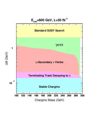
Search strategies for production with almost degenerate chargino and neutralino masses are discussed in [32]. The most critical ingredients are the lifetime and the decay modes of , which depend almost entirely on the small mass difference . (i) For the chargino may exit the detector as heavily ionising stable particle, or decay to a soft, but visible or yielding a secondary vertex. (ii) If GeV the may decay inside the tracking system to a soft , which need not be visible. The signature is a terminating track. (iii) For GeV the decay pion(s) will be detected, possibly associated to a secondary vertex. The large background from may be suppressed by requiring an additional tagged photon. If the pions have too low an energy to be detected, then one relies on a single photon signature from production, which, however, has a large background. (iv) Once GeV, the decay products have sufficient energy to be detected and resemble the usual MSSM topologies.
The AMSB discovery potential is shown in Fig. 1 as a function of and for GeV. With a large region can be covered almost to the kinematic limit. The discovery regions increase only slightly with higher luminosity, except for the channel, which would be extended beyond GeV accesible with low luminosity. Since GeV is typical of models with loop-dominated gaugino masses, the tagged signals are very important.
8 Supersymmetry with –Parity Violation
So far it has been assumed that the multiplicative quantum number –parity is conserved. Under this symmetry all standard model particles have and their superpartners . As a consequence, SUSY particles are only produced in pairs with the lightest of them (LSP) being stable, giving rise to missing energy in an experiment. In the MSSM, this is the neutralino .
–parity conservation has, however, no strong theoretical justification. The superpotential admits explicit –parity violating () terms such as [33]
| (1) |
where are the left–handed lepton and squark superfield and are the corresponding right–handed fields. If both lepton–number violating ( and ) and baryon–number violating () couplings were present, they would give rise to fast proton decay. This is avoided by assuming at most one coupling to be finite.
–parity violation changes the SUSY phenomenology drastically. The lightest supersymmetric particle decays, so the typical missing energy signature in the conserving MSSM is replaced by multi-lepton and/or multi-jet final states.
1 Single SUSY particle production
If –parity is violated, then single SUSY particle production is possible, for instance , which extends the accessible mass reach considerably. For sneutrino masses one expects spectacular resonances [34, 35]. Since the exchanged sneutrino carries spin 0, the signal can be further enhanced by polarising both the incoming electron and positron beams with the same helicities and thereby reducing any background mediated through exchange substantially [4].
If both production and decay occur via couplings, Bhabha scattering is particular sensitive to the interference with heavy sneutrino exchange diagrams [35]. This is illustrated in Fig. 2 in case of –channel resonance production. Masses beyond the center of mass energy are accessible via contact interactions. The effects scale as and one is sensitive to masses of TeV for a coupling of at the highest Tesla energy.


A detailed study of single chargino production with subsequent decays and , leading to a final state is presented in [36]. The production proceeds via exchange in the –channel and exchange in the –channel. Due to the coupling which flips helicity, production occurs through and production through . Figure 2 shows the distribution of the highest muon transverse momentum. Single chargino production can be easily separated from the background and the pronounced peak in can be used to reconstruct the mass. With at GeV, values of the coupling much smaller than present low–energy bounds can be probed for . The sensitivity strongly increases when approaching a resonance, e.g. via ISR radiation, where can be reached.
Other couplings are accessible via the LSP decays. A simulation of production with hadronic decays via coupling, which lead to 6 jets including 2 –quark jets, is presented in [37]. Exploiting the overconstrained kinematics of the final state, the SM and SUSY background can be efficiently reduced and the neutralino can be reconstructed with a mass resolution of for GeV.
A classification of violating signals in production, where the LSP decays via or couplings, is performed in [38]. The signature is an excess of events with at least three leptons plus missing energy or jets, which should be easily recognisable over the conserving MSSM and SM expectation.
2 Bilinear violation of –parity
A particularly simple form of –parity breaking is realised by additional bilinear couplings in the superpotential [39]
| (2) |
where and are the lepton and Higgs superfields. The electroweak symmetry is broken when the two Higgs doublets and and the neutral components of the slepton doublets acquire vacuum expectation values. The model breaks lepton number and generates non–zero Majorana neutrino masses, thus providing an elegant mechanism for the origin of neutrino masses. At tree–level only one of the neutrinos gets a mass by mixing with neutralinos, leaving the other two neutrinos massless. While this can explain the atmospheric neutrino problem, to reconcile it with the solar neutrino data requires going beyond the tree–level approximation. A full one–loop calculation of the neutralino–neutrino mass matrix consistent with solar and atmospheric neutrino data was performed in [40].
An interesting feature of this model is, that the semileptonic branching ratios of the neutralino decays and can be related to the atmospheric neutrino mixing , shown in Fig. 3 for a variety of model parameters. Note that in this class of theories neutrino mixing angles can be probed at accelerators.
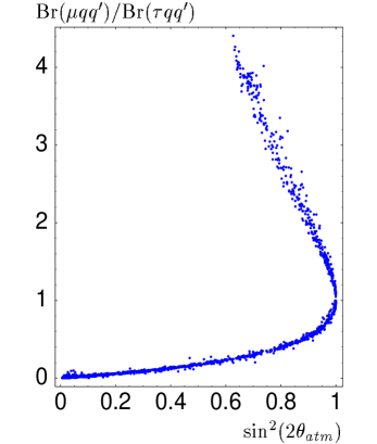
Another property of this model is that the light stop decays may indicate –parity violation [41]. The decay can be as important as the conserving three-body decays and the loop-decay . The main reason is that for the chargino mixes with the lepton. The corresponding mass region is GeV, where it might be difficult to detect the stop at the LHC.
9 , and Options
Additional information on the supersymmetry particle spectrum may be obtained when operating Tesla in the , and modes, each with highly polarised beams.
Supersymmetry in collisions is limited to selectron pair production via neutralino exchange. The main interest lies in mass determinations through threshold scans. Selectrons associated to the same helicity, and , are produced with angular momentum leading to a dependence of the cross section [42], in contrast to the less steep behaviour in collisions. This apparent advantage, however, is depleted by initial state radiation and beamstrahlung effects, which severely degrade the shape (flattening of the steep rise) and magnitude of the excitation curve at threshold [43]. Given the considerably lower luminosity, it is questionable whether on gets competitive or even more precise mass measurements in comparable running times. An interesting possibility is to search for mixing in the slepton sector (analogous to neutrino mixing) via lepton number violating decays , where electron collisions provide a very clean environment.
Higher selectron masses beyond the kinematic limit can be probed by associated production of . Further, this process offers an interesting possibility to access the gaugino mass parameter [44]. Using highly polarised electron and photon beams the cross sections are large and any ambiguities are easily resolved by measuring polarisation asymmetries. With moderate luminosities, the parameter can be determined within a per cent or better depending on the MSSM scenario. Such measurements combined with those from the chargino sector, see Table 1, allow a stringent test of the GUT relation .
In photon collisions the production of charged sfermions, sleptons or squarks, [45] and charginos [46] are pure QED processes and depend essentially on the sparticle masses and charges (interesting for squarks). Therefore, in contrast to annihilation, the decay mechanisms can be separated from the production, which simplifies an analysis of the relevant SUSY parameters. In general the polarised cross sections are larger than in annihilation up to the kinematic limit, thus allowing to study more subtle effects. Another interesting possibility is resonant stoponium production [47]. The cross section for collisions with total helicity 0 may be quite large and the dominant decay modes to gluons or Higgs pairs easily detectable. Such a resonance would be observable in annihilation at an appreciably lower rate only if the decay to Higgs bosons is dominant.
10 Extrapolation of SUSY Parameters to High Energy Scales
In most studies of SUSY models assumptions are made at a high energy scale. In the minimal supergravity model with the input parameters , , , , at the GUT scale GeV, all gauge couplings , all gaugino masses and all scalar masses unify at . In the GMSB model one starts from boundary conditions at the messenger scale for the gaugino and scalar masses. The evolution of the parameters down to the electroweak scale is described by the renormalisation group equations.
In order to test these assumptions and models one can also start from the particle spectrum measured at lower energies and extrapolate the corresponding SUSY parameters by RGE to higher energies. Such a ‘bottom–up’ approach is presented in [48]. They analyse in detail the mSUGRA point GeV, GeV GeV, and , which determines the particle spectrum at low energy. From fits to the mass spectrum and cross sections, as given by simulations of Tesla [5] and LHC [49, 50] experiments, one extracts the SUSY parameters including their correlated errors. Typical mass errors are given in Table 1.
| particle | m [GeV] | m [GeV] | |
| LHC | LHC+LC | ||
| 109 | 0.2 | 0.05 | |
| 259 | 3 | 1.5 | |
| 133 | 3 | 0.11 | |
| 72.6 | 3 | 0.15 | |
| 233 | 3 | 0.1 | |
| 217 | 3 | 0.15 | |
| 214 | 3 | 0.8 | |
| 154 | 3 | 0.7 | |
| 466 | 10 | 3 | |
| 377 | 10 | 3 | |
| 470 | 10 | 10 | |
The extrapolation of the corresponding SUSY parameters from the weak scale to the GUT scale within the mSUGRA scenario are shown in Fig. 1. It can be seen that the gaugino mass parameters and the slepton mass parameters for the first and second generation are in excellent agreement with unification, due to the precise measurements in the slepton and chargino/neutralino sectors. Using only LHC information would give uncertainties on the unification scale worse by more than an order of magnitude. The squark parameters and the Higgs parameter , being less well known, still allow to test unification.
To confront the mSUGRA scenario with an alternative one, the analysis was also done for the GMSB model with the parameters TeV, TeV, , and . The results are shown in Fig. 2. Note that approaches the parameter for at the GMSB scale around GeV as both belong to weak isodoublet fields which do not have strong interaction. As one can see one gets a very different picture at high energy scales compared to the mSUGRA model, and obviously both scenarios cannot be confused. Moreover, from both Fig. 1 and Fig. 2 one can see that precision data are essential for stable extrapolations to high energy scales.
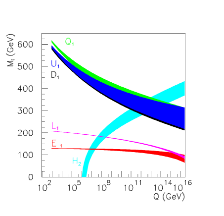
11 Comparison of TESLA with LHC
If supersymmetry is realized at low energies, it will be discovered at the LHC. In particular, squarks and gluinos – if they exist – will be produced abundantly because of their strong interaction. It will be possible to discover gluinos and squarks up to a mass of 2.5 TeV by a variety of distinctive signatures (multiple jets, multi-leptons, etc. + missing energy) [49, 50]. However, at LHC all kinematically accessible SUSY particles (charginos, neutralinos, sleptons) are produced simultaneously either directly or in cascade decays of gluinos and squarks. It is extremely difficult and often impossible to separate the many SUSY processes which can occur. A model independent experimental analysis, aiming at a measurement of the masses and other properties of the particles, is essentially precluded. In most cases, one has to invoke model assumptions and to compare the predictions with the experimental distributions. By selecting decay chains, e.g. , it is possible to construct enough kinematic constraints to determine the masses of the primary and daughter particles. Such studies have been performed in a variety of SUSY scenarios [49, 50], covering a large range of model parameters.
Concerning the mass reach, LHC has of course a larger discovery potential for almost all SUSY particles than Tesla due to the high centre of mass energy and will be able to determine particle masses in given scenarios with an accuracy of a few percent. Other sparticle properties, however, remain almost inaccessible.
Tesla, on the other hand, offers far superior measurements of the SUSY particle spectrum wihin its energy range, specifically:
-
•
a precise determination of particle masses:
= 0.1 – 1 GeV, = 0.05 – 0.3 GeV, = 0.6 GeV, = 1 GeV.
The high accuracy of masses allows the extrapolation to very high energies (GUT scale) revealing the origin of SUSY breaking. -
•
precise measurement of the widths and branching ratios
-
•
precise determination of the couplings
-
•
determination of the mixing parameters in the chargino/neutralino sectors
-
•
measurement of the mixing angles in the and sectors
-
•
determination of in the sector if
-
•
determination of the spin and the quantum numbers
-
•
model independent determination of SUSY parameters
-
•
measurement of CP violating phases
It should be emphasised that for all these precision measurements the use of polarised beams is important. Polarised in addition to polarised are especially useful for the separation of and in production, and in –parity violating analyses.
Only via the precision measurements which are possible at Tesla can the underlying SUSY model be revealed and its parameters determined. The input of findings from the LHC will of course be valuable for experimentation at Tesla. It is worth pointing out that precise measurements from Tesla, particularly of the masses of the LSP and sleptons, would greatly improve the quality of the information which LHC can derive from multiple decay chains.
To summarise, from these comparisons it is obvious that the LHC and Linear Collider programmes complement each other. The LHC may discover supersymmetry and constrain its gross features. However, only high precision measurements at the Tesla Linear Collider will be able to pin down the detailed structure of the underlying supersymmetry theory.
References
-
[1]
For Reviews see: H.P. Nilles. Phys. Rept., 110:1, 1984;
H.E. Haber and G.L. Kane. Phys. Rept., 117:75, 1985. -
[2]
See e.g. DESY Series of Linear Collider Workshops: DESY 92–123A,
DESY 92–123B, DESY 93–123C, DESY 96–123D, DESY 97–123E;
E. Accomando et al. Phys. Rep., 299:1, 1998. -
[3]
2nd Joint ECFA/DESY Study on ‘Physics and Detectors for a Linear
Electron–Positron Collider’,
http://www.desy.de/conferences/ecfa-desy-lc98.html;
SUSY working group: http://wwwhephy.oeaw.ac.at/susy/lcws.html. - [4] G. Moortgat-Pick and H. Steiner. Beam Polarization at a Linear Collider: What do we gain with Positron Polarization. LC–TH–2000–055, 2000. http://www.desy.de/~lcnotes/. electronic document.
-
[5]
H.-U. Martyn and G.A. Blair. In Proceedings of ‘Physics and Experiments with
Future Linear Colliders’, Sitges, Spain, 1999, ISBN 84-490-1977-X;
H.-U. Martyn and G.A. Blair. Determination of Sparticle Masses and SUSY Parameters. LC–TH–2000–023, 1999. http://www.desy.de/~lcnotes/. electronic document. -
[6]
H.-U. Martyn. In ’Physics at TeV Colliders’, Les Houches, France, 1999;
H.-U. Martyn. Width Effects in Slepton Production . LC–TH–2000–024, 1999. http://www.desy.de/~lcnotes/. electronic document, hep-ph/0002290. - [7] J. Feng and D. Finnell. Phys. Rev., D49:2369–2381, 1994. electronic document, hep-ph/9310211.
- [8] A. Freitas, D. Miller, and P. Zerwas. Finite Width Effects and Gauge Invariance in Slepton Pair Production. LC–TH–2001–011, 2000. http://www.desy.de/~lcnotes/. electronic document.
- [9] M. Nojiri, K. Fujii, and T. Tsukamoto. Phys. Rev., D54:6756–6776, 1996. electronic document, hep-ph/9606370.
- [10] T. Kamon. Proceedings of the 5th Int. Workshop on Physics and Experiments with Future Linear Colliders (LCWS 2000), Fermilab, Illinois, USA, 2000, to be published. see also http://conferences.fnal.gov/lcws2000.
- [11] S. Choi, et al. Eur. Phys. J., C14:535–546, 2000. electronic document, hep-ph/0002033.
- [12] G. Moortgat-Pick, A. Bartl, H. Fraas, and W. Majerotto. Beam Polarization and Spin Correlation Effects in Chargino Production and Decay. LC–TH–2000–033, 1999. http://www.desy.de/~lcnotes/. electronic document, hep-ph/0004181.
- [13] T. Blank and W. Hollik. Radiative Corrections to Chargino Production in Electron Positron Collisions. LC–TH–2000–054, 2000. http://www.desy.de/~lcnotes/. electronic document, hep-ph/0011092.
-
[14]
G. Moortgat-Pick, A. Bartl, H. Fraas, and W. Majerotto. Eur. Phys. J.,
C(7):113, 1999;
electronic document
G. Moortgat-Pick, A. Bartl, H. Fraas, and W. Majerotto. Exploiting Spin Correlations in Neutralino Production and Decay with Polarized e- e+ Beams. LC–TH–2000–032, hep-ph/0002253. http://www.desy.de/~lcnotes/. electronic document. -
[15]
S. Hesselbach, F. Franke, and H. Fraas. Neutralino Production with Polarized
Beams in Extended Supersymmetric Models. LC–TH–2000–025,
hep–ph/0003272; http://www.desy.de/~lcnotes electronic document
S. Hesselbach, F. Franke, and H. Fraas. Phys. Lett., B492:140, 2000. electronic document. -
[16]
J.L. Kneur and G. Moultaka. Phys. Rev., D59:015005, 1999;
J.L. Kneur and G. Moultaka. Phys. Rev., D61:095003, 2000. - [17] A. Bartl, H. Eberl, S. Kraml, W. Majerotto, and W. Porod. Phenomenology of Stops, Sbottoms, Tau Sneutrinos, and Staus at an Linear Collider. LC–TH–2000–031, 2000. http://www.desy.de/~lcnotes/. electronic document, hep-ph/0002115.
-
[18]
M. Drees, K.I. Hikasa. Phys. Lett., B252:127, 1990;
W. Beenakker, R. Höpker, and P.M. Zerwas. Phys. Lett., B349:463, 1995; electronic document
K.I. Hikasa and J. Hisano. Phys. Rev., D54:1908, 1996. electronic document. - [19] H. Eberl, A. Bartl, and W. Majerotto. Nucl. Phys., B472:481–494, 1996. electronic document, hep-ph/9603206.
- [20] H. Eberl, S. Kraml, and W. Majerotto. JHEP, 05:016, 1999. electronic document, hep-ph/9903413.
-
[21]
R. Keranen, A. Sopczak, H. Nowak, and M. Berggren. EPJdirect, C(7):1,
2000. LC–PHSM–2000–026; http://www.desy.de/~lcnotes electronic document
A. Sopczak and H. Nowak. Proceedings of the 5th Int. Workshop on Physics and Experiments with Future Linear Colliders (LCWS 2000), Fermilab, Illinois, USA, 2000, to be published. electronic document. - [22] S. Abdullin et al. ‘Physics at TeV Colliders’, Les Houches, France, 1999: The SUSY Working Group Summary Report, 1999. electronic document, hep-ph/0005142.
- [23] S. Heinemeyer and G. Weiglein. Electroweak Precision Tests with GigaZ. LC–TH–2001–001, 2000. http://www.desy.de/~lcnotes/. electronic document, hep-ph/0012364.
- [24] K. Hikasa and M. Kobayashi. Phys. Rev., D36:724, 1987. electronic document.
-
[25]
W. Porod and T. Wöhrmann. Phys. Rev., D(55):2907, 1997.
electronic document
W. Porod. Phys. Rev., D(59):095009, 1999. electronic document. -
[26]
C. Boehm, A. Djouadi, and Y. Mambrini. Phys. Rev., D61:095006, 2000;
electronic document
A. Djouadi and Y. Mambrini. Higher–Order Decays of the Lightest Top Squark. LC–TH–2000–029, 2000. http://www.desy.de/~lcnotes electronic document. - [27] M. Drees. Dark matter and the SUSY Mass Scale. LC–TH–2001–013, 2001. http://www.desy.de/~lcnotes/. electronic document, hep-ph/0101217.
- [28] M. Dine, A. Nelson, and Y. Shirman. Phys. Rev., D51:1362–1370, 1995. electronic document, hep-ph/9408384.
- [29] S. Ambrosanio and G. Blair. Eur. Phys. J., C12:287–321, 2000. LC–TH–1999–019. http://www.desy.de/~lcnotes electronic document, hep-ph/9905403.
- [30] L. Randall and R. Sundrum. Nucl. Phys., B557:79–118, 1999. electronic document, hep-th/9810155.
- [31] G. Giudice, M. Luty, H. Murayama, and R. Rattazzi. JHEP, 12:27, 1998. electronic document, hep-ph/9810442.
- [32] J. Gunion and S. Mrenna. Probing Models with Near Degenracy of the Chargino and LSP at the Linear Collider. LC–TH–2001–012, 2000. http://www.desy.de/~lcnotes/. .
- [33] L. Hall and M.Suzuki. Nucl. Phys., B231:419, 1984. electronic document.
- [34] S. Lola. Resonant Single Chargino and Neutralino versus Fermion Antifermion Production at the Linear Collider. LC–TH–1999–021, 1998. http://www.desy.de/~lcnotes/. electronic document, hep-ph/9912217.
- [35] M. Heyssler, R. Rückl, and H. Spiesberger. In Proceedings of ‘Physics and Experiments with Future Linear Colliders’, Sitges, Spain, 1999, ISBN 84-490-1977-X. electronic document, hep-ph/9908319.
- [36] G. Moreau. Single Chargino Production at Linear Colliders. LC–TH–2000–040, 2000. http://www.desy.de/~lcnotes/. electronic document, hep-ph/0009140.
- [37] M. Besancon and G. Moreau. In Proceedings of ‘Physics and Experiments with Future Linear Colliders’, Sitges, Spain, 1999, ISBN 84-490-1977-X. electronic document, hep-ph/9909441.
- [38] D. Ghosh, R. Godbole, and S. Raychaudhuri. Signals for Charginos and Neutralinos in R–Parity Violating Supersymmetric Theory at a 500 GeV Collider. LC–TH–2000–051, 2000. http://www.desy.de/~lcnotes/. electronic document.
- [39] M. Díaz, J. Romão, and J. Valle. Nucl. Phys., B524:23–40, 1998. electronic document, hep-ph/9706315.
-
[40]
M. Hirsch, M.A. Díaz, W. Porod, J.C. Romão, and J.W.F. Valle. Phys. Rev. D62:113008, 2000;
electronic document
M. Hirsch, M.A. Díaz, W. Porod, J.C. Romão, and J.W.F. Valle. Phys. Rev. D61:071703, 2000. electronic document. - [41] W. Porod, D. Restrepo, and J. Valle. Light Stop: MSSM Versus R-Parity Violation. LC–TH–2000–005, 2000. http://www.desy.de/~lcnotes/. electronic document, hep-ph/0001033.
- [42] J. Feng. Int. J. Mod. Phys., A13:2319–2328, 1998. electronic document, hep-ph/9803319.
- [43] C. Heusch. Talk at LCWS 2000, FNAL, October 2000.
- [44] C. Blochinger and H. Fraas. Possible Test of the GUT Relation between M1 and M2 in Electron Photon Scattering. LC–TH–2000–017, 2000. http://www.desy.de/~lcnotes/. electronic document, hep-ph/0001034.
- [45] S. Berge, M. Klasen, and Y. Umeda. Phys. Rev., D63:35003, 2001. electronic document, hep-ph/0008081.
- [46] T. Mayer and H. Fraas. Chargino Production and Decay in Photon Photon Collisions, 2000. electronic document, hep-ph/0009048.
- [47] D. Gorbunov, V. Ilyin, and V. Telnov. TESLA: Potentials of Gamma Gamma and e+ e- Options in Stoponium Searches, 2000. electronic document, hep-ph/0012175.
- [48] G. Blair, W. Porod, and P. Zerwas. Phys. Rev., D63:17703, 2001. electronic document, hep-ph/0007107.
-
[49]
I. Hinchliffe et al. Phys. Rev., D55:5520, 1997;
electronic document
ATLAS: Detector and Physics Performance Technical Design Report, Volume 2. CERN/LHCC/99–15, ATLAS TDR 15. - [50] S. Abdullin et al. Discovery Potential for Supersymmetry in CMS. CMS Note 1998/006, 1998. electronic document, hep-ph/9806366.
Chapter 3 Alternative Theories
1 Introduction
Microscopic physics is characterized in the standard formulation by two scales, the electroweak scale of order GeV at which the Standard Model is defined, and the Planck scale of order GeV where particle physics and gravity are linked. The large gap between the two scales can be stabilized by supersymmetry. This picture of Nature is strongly supported by the successful prediction of the electroweak mixing angle; however, alternative scenarios are not ruled out.
1.) Extending the Minkowski–Einstein Universe by extra space dimensions not near the Planck scale but at semi-macroscopic scales may change the picture dramatically [Antoniadis; Arkani-Hamed, Dimopoulos, Dvali]. Gravity may become strong in extended space already at the TeV scale and the hierarchy problem, present in the standard picture, is non-existent. Towers of Kaluza–Klein states are realized on the compactified extra dimensions which affect high-energy processes, giving rise to missing-energy signals and new contact interactions, or novel resonances with masses in the TeV range.
The large gap between the scales may also be generated by localizing gravity on a wall different from the wall of the Standard Model in higher space-time dimensions [Randall-Sundrum]. The projection of gravity down to the SM wall is weak, the large Planckian energy scale being reduced exponentially. Kaluza–Klein graviton resonances should be observed at the TeV scale in such a scenario.
Even though all these ideas are highly hypothetical, they open new vistas, in particular on the unsolved theoretical problems in gravity. Observation of effects in high-energy experiments as described above, would revolutionize the basic space-time picture of the world.
2.) So long as the Higgs mechanism is not established firmly, rival theories for generating the masses of the fundamental particles in the Standard Model must be considered seriously. In the standard Standard Model the masses are generated by interactions of the particles with the fundamental Higgs field, being of non-zero field strength in the ground state as a result of spontaneous symmetry breaking. Alternatively, the symmetry breaking could be of dynamical origin as realized in theories of new strong interactions at the TeV scale [Susskind, Weinberg]. The masses of the gauge fields are generated by absorption of Goldstone bosons associated with the breaking of global symmetries.
In such scenarios, the bosons become strongly interacting particles at high energies. This will affect the production of pairs in annihilation, and the amplitudes for scattering in the threshold region of the strong interactions can be predicted. From both effects the scale of the new strong interactions can be determined at a sub-TeV collider. New resonances will be observed in the (multi-)TeV mass range. Extending these ideas to fermions generates quite a number of serious difficulties, inflicted by the necessary coexistence of disgruent large scales. They require rather complex theoretical constructs in attempts to solve these problems.
3.) Strong interactions between particles have signalled quite often in the past, hidden composite structures. Solving the problem of mass by new strong interactions naturally raises the question of non-pointlike structures of electroweak gauge bosons, leptons and quarks. Analyzing contact interactions in high-energy scattering experiments will probe or set bounds on the radii of these particles. The same compositeness picture suggests leptoquarks as novel bound states.
Experimentation at TESLA may thus open vistas to new physics areas, “unexpected” in the standard form of non-standard physics.
2 Extra Dimensions
A novel approach which exploits the geometry of extra spatial dimensions has recently been proposed [1, 2, 3, 4] as a means of addressing the gauge hierarchy (for a different approach to the link between electroweak symmetry breaking and gravity see Ref. [5]). These models make use of the fact that gravity has yet to be probed at energy scales much above eV in laboratory experiments. In the scenario of Arkani–Hamed, Dimopoulos and Dvali [1], the apparent hierarchy is generated by a large volume for the extra dimensions, while in the Randall–Sundrum model [3], the observed hierarchy is created by an exponential warp factor which arises from the localization of gravity in a 5-dimensional non-factorizable geometry. Moreover, recent theoretical results have demonstrated that non-commutative field theories naturally appear within the context of string/M-theory [4]. An exciting feature of these three classes of theories is that they afford concrete and distinctive phenomenological, as well as astro-physical, tests. Furthermore, if they truly describe the source of the observed hierarchy, then their signatures should appear in experiments at the TeV scale. We now review these models and discuss their signatures at the TESLA collider.
1 Gravity at large dimensions
In the scenario of Ref. [1], gravitational interactions become strong near the weak scale and take place mainly in new large spatial dimensions, known as the bulk. Since it is known experimentally that the Standard Model fields do not feel the effects of extra dimensions with a compactification scale of less than a few TeV, they are constrained to lie on a -dimensional brane, or wall, in the higher dimensional space. Gravity thus appears weak in ordinary 4-dimensional space-time as we only observe its projection onto the wall. The relation between the scales where gravity becomes strong in the and 4-dimensional theories can be derived from Gauss’s Law and is given by , where denotes the fundamental Planck scale in the higher dimensional space, and is the volume of the compactified dimensions. Setting TeV thus determines the size of the extra dimensions for a given value of . The case of is ruled out by astronomical data. Cavendish-type experiments have excluded departures from the gravitational inverse square law for length scales exceeding 190 m [6]. For this rules out TeV using the mass-scale convention of [7]. In addition, astro-physical and cosmological considerations [8], such as the rate of supernova cooling and the -ray flux spectrum, disfavor a value of near the TeV scale for .
The Feynman rules for this scenario [7, 9] are obtained by considering a linearized theory of gravity in the bulk. Upon compactification, the bulk gravitational field expands into Kaluza-Klein (KK) towers of gravitons, which are equally spaced and have masses of where labels the KK excitation level and denotes the radius of the compactified extra dimensions. Taking TeV, we see that the KK state mass splittings are equal to eV, 20 keV and 7 MeV for and 6, respectively. Note that due to the form of the action the spin-1 KK states do not interact with the wall fields, and that the scalar states are phenomenologically irrelevant for most processes at the TESLA collider. Each state in the spin-2 KK tower, , couples identically to the Standard Model wall fields via the stress energy tensor and the strength of the couplings is given by the inverse 4-d Planck scale, .
Graviton emission
There are two classes of collider signatures for gravity at large dimensions, with the first we discuss being that of graviton KK tower emission in scattering processes [7, 10]. The signal process at the TESLA collider is , where the graviton appears as missing energy in the detector as it behaves as if it were a massive, non-interacting, stable particle. The cross section is computed for the production of a single massive graviton excitation, and then summed over the full tower of KK states. Since the mass splittings of the KK excitations are quite small compared to the collider center of mass energy, this sum can be replaced by an integral weighted by the density of KK states and which is cut off by the specific process kinematics. This has the effect of removing the 4-d Planck scale suppression; the factor which appears from the graviton couplings is exactly cancelled by the dependence of the phase space integration. The process now scales as simple powers of . It is important to note that due to the effective density of states, the emitted graviton appears to have a continuous mass distribution; this corresponds to the probability of emitting gravitons with different momenta in the extra dimensions. The differential cross-section of is given [7] by
| (1) |
where , is the number of extra dimensions and is the surface area of a -dimensional sphere of unit radius, with
| (2) |
The discovery reach of the TESLA collider for direct graviton production in is estimated for an integrated luminosity of 1 ab-1 at GeV. Details of these studies are given in [11] and [12]. The signature is a relatively soft photon and missing energy. The major background is and it is largely irreducible. The following kinematic acceptance cuts are imposed on the photon:
-
•
Within the acceptance of the electromagnetic calorimeter, .
-
•
in order to reject events with no genuine missing such as where electrons at polar angles below the mask calorimeter acceptance of 27.5 mrad mimic missing .
-
•
in order to reject the energetic photons from which arise from .
With these cuts, the accepted cross-sections including ISR and beamstrahlung from for 100% electron polarisation are pb and fb, evaluated using NUNUGPV [13]. The cross section for left-handed electrons is much enhanced due to the dominance of exchange contributions in this kinematic region. Other backgrounds have so far been neglected; they will be small but should not be ignored, e.g. . For the signal, as an example for TeV and , the unpolarised accepted Born cross-section without beamstrahlung is 12 fb.
Given the near maximal polarisation asymmetry of the background, polarised beams of appropriate helicity are extremely effective in suppressing the background and therefore extending the reach of the TESLA collider in the quest for evidence of extra dimensions. Fig. 1 compares the signal cross-sections with the background cross-sections for several polarisation assumptions. Numerical sensitivity estimates shown here are based on a normalisation uncertainty of 0.3%. For completeness, the studies in [11, 12] have also considered normalisation uncertainties varying from 0.1% (optimistic) to 1.0% (conservative). Many sources of systematic error will have to be controlled at quite challenging levels of precision: theoretical error on background cross-section, absolute luminosity, selection efficiency, energy scale and polarisation. However the availability of large control data-sets such as and should allow detector related systematics to be kept under sufficient control.

The inclusive cross-section measurement is used to estimate the sensitivity. A modest improvement is expected if information on the energy and polar angle distributions is also included. The sensitivity estimates are shown in Table 1 for numbers of extra dimensions ranging from 2 to 6. By polarising both beams to a high degree, the TESLA collider potential for exploring this physics is maximised.
| 2 | 3 | 4 | 5 | 6 | |
|---|---|---|---|---|---|
| 5.9 | 4.4 | 3.5 | 2.9 | 2.5 | |
| 8.3 | 5.8 | 4.4 | 3.5 | 2.9 | |
| 10.4 | 6.9 | 5.1 | 4.0 | 3.3 |
At the LHC, direct graviton production can be explored using the signature of . However for certain values of (), the partonic centre-of-mass energy can exceed and the effective low energy theory approach breaks down at LHC. A recent study [15] of the LHC potential with the ATLAS experiment shows that in 100 fb-1, direct graviton production can be discovered at at least for in the ranges shown in Table 2 for and 4. However the effective theory approach breaks down at LHC for and for values below the given ranges when 2,3 and 4. At TESLA, if the effective theory approach should be valid and the measured single photon cross-section can be used to constrain (). TESLA offers a more model-independent test of this theory while the LHC may be in the string theory regime whose phenomenology is perhaps rich but presently unknown. For regions which can be compared, as shown in Table 2, the 5- discovery reach in for TESLA and the LHC is similar.
| 2 | 3 | 4 | 5 | 6 | |
|---|---|---|---|---|---|
| LHC | 4.0—7.5 | 4.5—5.9 | 5.0—5.3 | none | none |
| TESLA | 0.5—7.9 | 0.5—5.6 | 0.5—4.2 | 0.5—3.4 | 0.5—2.9 |
Anomalous single photon signatures at TESLA and monojet signatures at LHC can both arise from many types of new physics other than extra dimensions. Therefore measurement of processes sensitive to direct graviton production with complementary initial and final states would help to confirm whether the correct diagnosis had been made. At TESLA, the process can be explored in collisions; however the sensitivity relative to is rather limited [16]. A more promising channel is [17].
If extra dimensions are the cause of the anomalous single photon rate, the dependence of the cross-section should follow . Fig. 2 illustrates how a measurement of an excess of single photon events at GeV together with a measurement at GeV can be used to determine the number of extra dimensions. Determination of the number of extra dimensions is possible with this data-taking scenario for excess cross-sections at 500 GeV down to fb. This cross-section is equivalent to TeV for and for these values, one would exclude on average at 99% CL. Inconsistency with the expected dependence, i. e. excluding integer values of , would exclude the extra dimensions interpretation.
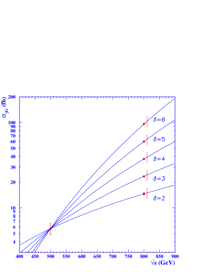
The LHC and TESLA therefore have valuable complementary roles to play in experimentally testing theories with extra space dimensions.
Virtual effects
The second class of processes considered here is that of graviton exchange [7, 9, 18] in scattering. This virtual exchange mechanism leads to deviations in cross sections and asymmetries in Standard Model processes, such as , and can also mediate new processes which are not present at tree-level in the Standard Model, such as or . The exchange amplitude is proportional to the sum over the propagators for the entire graviton KK tower and, again, can be converted to an integral over the density of states. However, in this case the integral is divergent for and thus introduces a sensitivity to the unknown ultraviolet physics. Several approaches have been proposed to regulate this integral. Here, we adopt the most model independent approach, that of a naive cut-off [7, 9, 18], and set the cut-off equal to . Assuming that the integral is dominated by the lowest dimensional local operator, which is dimension-8, this results in a contact-type interaction limit for graviton exchange. This is described in the matrix element for -channel scattering by the replacement
| (3) |
with corresponding substitutions for - and -channel scattering. Here represents the reduced Planck scale , is the mass of the nth graviton KK excitation, and is a model dependent factor, which we take to be of order unity and of either sign. This substitution is universal for all final states. The resulting angular distributions for fermion pair production are quartic in and thus provide a unique signal for spin-2 exchange. We present an example of this in Figs. 4 and 4 which display the angular distribution and Left-Right asymmetry in production for TeV and GeV. The two dashed histograms correspond to the two choices of sign for . Table 3 presents the sensitivities in in final states. Combining all final states TESLA will be sensitive up to TeV at GeV [19].


| [TeV] | ||
| TeV | TeV | |
| 4.1 | 5.8 | |
| 5.0 | 7.1 | |
| 5.1 | 7.1 | |
| combined | 5.6 | 8.0 |
It should be noted that the best limits, as phenomenologically calculated, on in the model of Ref. [1] may arise from virtual graviton exchange in . The reach in at a collider can be estimated to be about [20].
In a certain class of models with extra dimensions compactified at the TeV scale the SM fields can also explore the extra dimensions [2, 21]. For extra dimensions this translates into a fundamental quantum gravity scale of about 8000 TeV. This scenario can lead to superparticle mass of the order of the electroweak scale. Since the scale is large, direct quantum effects of gravity will be inaccessible at TESLA. However, these models exhibit spin 1 excitation states of the SM gauge bosons , called “Kaluza–Klein recurrences”. By means of the process TESLA can reach a sensitivity in the compactification scale beyond 10 TeV at high energy and high luminosity [21] [corresponding to scales TeV for ]. This turns out to be significantly larger than the sensitivity TeV, which can be reached at the LHC by means of dilepton production [21].
2 Randall–Sundrum model
In the Randall–Sundrum model the hierarchy is generated by an exponential function of the compactification radius. In its simplest form, this model consists of a 5-dimensional non-factorizable geometry based on a slice of Anti-de-Sitter (AdS5) space of length , where denotes the compactification radius. Two 3-branes, with equal and opposite tensions, reside rigidly at orbifold fixed points at the boundaries of the AdS5 slice. The 5-dimensional Einstein’s equations permit a solution which preserves 4-d Poincaré invariance with the metric
| (4) |
where . Here, is the AdS5 curvature scale which is of order the Planck scale and is determined by the bulk cosmological constant , where is the 5-d Planck scale. Examination of the 4-d effective action yields . The scale of physical phenomena as realized by the 4-d flat metric transverse to the 5th dimension is specified by the exponential warp factor. TeV scales can naturally be attained on the 3-brane at if gravity is localized on the Planck brane at and . The scale of physical processes on this TeV-brane is then TeV. It has been demonstrated [22] that this value of can be stabilized without the fine tuning of parameters.
The 4-d phenomenology of this model is governed by 2 parameters, and the ratio , where constraints on the 5-d curvature suggest that . The Feynman rules are also obtained by a linear expansion of the flat metric, which in this case includes the warp factor. On the TeV-brane, the resulting KK tower of gravitons now have masses given by with the being the roots of the first-order Bessel function, i.e. . Note that the first excitation is naturally of order a few hundred GeV and that the KK states are not evenly spaced. Due to the explicit form of the interactions of the KK tower with the Standard Model fields on the TeV-brane the zero-mode decouples and the excitation state couplings are now an inverse TeV. This results in a strikingly different phenomenology than in the above case of large extra dimensions, as now the graviton KK tower states can undergo single, direct, resonance production. To exhibit how the tower of graviton excitations may appear at the TESLA collider, Fig. 5 displays the cross section for as a function of , assuming GeV and taking various values of for purposes of demonstration. Searches for the first KK resonance in Drell-Yan and di-jet data at the Tevatron already place non-trivial constraints [23] on the parameter space of this model. If the KK gravitons are too massive to be produced directly, their contributions to fermion pair production may still be felt via virtual exchange. Since in this case there is only one additional dimension, the uncertainties associated with the introduction of a cut-off do not appear, as opposed to the model of Ref. [1] as discussed above. As shown in Ref. [23], scales of order TeV may be excluded for at a 500 GeV TESLA collider with 500 fb-1 of integrated luminosity. Lastly, we note that if the Standard Model fields are also allowed to propagate in the bulk [24], the phenomenology can be markedly different, and is highly dependent upon the value of the 5-dimensional fermion mass, which is of order of the Planck mass and thus different from the effective fermion mass in 4 dimensions.
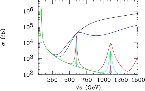
3 Non-commutative quantum field theory (NCQFT)
In models of NCQFT the usual -dimensional space associated with commuting space-time coordinates is generalized to one which is non-commuting. In such a space the conventional coordinates are represented by operators which no longer commute,
| (5) |
Here, we have parameterized the effect in terms of an overall scale , which characterizes the threshold where non-commutative (NC) effects become important, and a real antisymmetric matrix , whose dimensionless elements are presumably of order unity. The most likely value of is probably near the string or Planck scale, however, given the possibility of the onset of stringy effects at the TeV scale, and that the fundamental Planck scale may be lower due to the existence of large extra dimensions as discussed above, it is feasible that NC effects could also set in at a TeV. There is a clear relation between the matrix and the Maxwell field strength tensor as NCQFT arises in string theory through the quantization of strings as described by the low energy excitations of D-branes in the presence of background electromagnetic fields111NCQFT has been formulated so far only for QED. Extensions to SU(N) theories including quarks are studied presently.,222Astrophysical bounds have not been derived so far in a consistent way.. is identical in all reference frames, defining a preferred NC direction in space, and hence Lorentz invariance is violated at energies of order . However, due to the rotation of the Earth and its revolution about the Sun, the violation of Lorentz invariance is only observable in processes which are quadratic (or higher order even powers) in .
A striking consequence of NCQFT is that the NC version of QED takes on a non-abelian nature in that both 3-point and 4-point photon couplings are generated. In addition, all QED vertices pick up additional phase factors which are dependent upon the momenta flowing through the vertex. NCQED thus has striking effects in QED processes at the TESLA collider. The modifications to pair annihilation, Bhabha and Møller scattering, as well as have been studied in Ref. [25]. Pair annihilation and scattering both receive new diagrammatic contributions due to the non-abelian couplings, and all four processes acquire a phase dependence due to the relative interference of the vertex kinematic phases. The lowest order correction to the Standard Model to these processes occurs at dimension 8. The most interesting result is that a angular dependence is induced in scattering processes due to the existence of the NC preferred direction in space-time. This azimuthal dependence in pair annihilation is illustrated in Fig. 6 for the case where the NC direction is perpendicular to the beam axis. The results of Ref. [25] are summarized in Table 4 which displays the CL search reach for the NC scale in these four reactions. We see that these processes are complementary in their ability to probe different structures of non-commuting space-time. These results indicate that NCQED can be probed to scales of order a TeV, which is where one would expect NCQFT to become relevant if stringy effects of the fundamental Planck scale are also at a TeV.
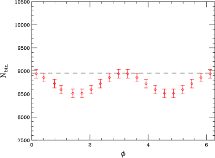
| Process | Structure Probed | Bound on |
|---|---|---|
| Space-Time | GeV | |
| Møller Scattering | Space-Space | 1700 GeV |
| Bhabha Scattering | Space-Time | 1050 GeV |
| Space-Time | GeV | |
| Space-Space | 500 GeV |
3 Strong Electroweak Symmetry Breaking
In the absence of a light Higgs particle or other low lying resonances, unitarity requires that the interaction among gauge bosons becomes strong at high energies. In this case, the physics of electroweak symmetry breaking (EWSB) below the symmetry breaking scale is described by the most general effective Lagrangian for the Goldstone bosons required by the spontaneous breaking. This Lagrangian describes the physics of longitudinal gauge bosons and its parameters can be probed in their interactions. Effective field theory allows to explore the multidimensional parameter space systematically, where the course of this exploration is laid out using power counting, dimensional analysis and symmetry.
All deviations of the -parameter from the minimal Standard Model tree level value of unity that have been observed by the LEP1/SLC experiments can naturally be accounted for by loop corrections in the minimal Standard Model itself. Therefore, the EWSB sector appears to have an approximate global custodial symmetry, protecting the -parameter from renormalisation, that is only broken by the hypercharge couplings of the Goldstone bosons. Hence it is reasonable to look for possible -conserving deviations from the Standard Model predictions first.
The luminosity and centre of mass energy of TESLA will allow experiments to probe the interactions of weak gauge bosons with unprecedented precision, so that the nature of EWSB can be determined even in a scenario without light resonances. For this purpose, the couplings of three gauge bosons and can be studied comprehensively in the production of four-fermion final states, using methods established at LEP2. The interactions of four gauge bosons can be analysed by disentangling the final states , , , and in six fermion production . A convenient basis for the analysis of weak gauge boson scattering is provided by the weak isospin channels. This analysis can be completed by measuring the purely channel , which is accessible in the mode of TESLA. Finally, GigaZ will contribute substantially improved limits on LEP1/SLC oblique corrections, which will provide the best constraints in one direction of parameter space.
In addition to model independent analyses of effective Lagrangians for the EWSB sector, specific models for the EWSB can be studied. These models typically include vector and scalar resonances, whose properties can be determined at TESLA.
1 Strong WW Interactions
Assuming only spontaneous symmetry breaking, the most general ( and conserving) effective Lagrangian contains 10 dimension-four interactions [26]. As mentioned above, appears to be conserved in EWSB and a natural strategy for multiparameter fits is to start the systematic exploration with the invariant333The operators are explicitely invariant, but they do contribute to the renormalisation of the violating dimension-two operator [26, 27]. This induces a deviation of the -parameter from unity at loop level, but the resulting limits on from LEP1/SLC are not competitive with the direct measurements discussed below. and linearly breaking operators. In the notation of [26], these are
| (1a) | ||||
| (1b) | ||||
| (1c) | ||||
| (1d) | ||||
| (1e) | ||||
where and simplifies to in unitarity gauge. The remaining five operators consist of four that break quadratically with two explicit s and one that breaks it quartically with four explicit s. Since appears to be approximately conserved in EWSB, its breaking must be governed by a higher scale , probably related to flavour physics. Then each explicit is naturally suppressed by one power of a small ratio . This observation justifies to start the exploration with the operators (1). The coefficients in (1) are related to scales of new physics by naive dimensional analysis (NDA) [28]
| (2) |
where the Fermi scale is fixed by low energy weak interactions. In the absence of resonances that are lighter than , one expects from NDA in a strongly interacting symmetry breaking sector
| (3) |
unless some couplings are naturally suppressed by symmetries (e. g. ). Therefore, the crucial benchmark for a linear collider from strong EWSB physics is given by this natural size of the couplings, in order to be able to probe the EWSB sector in any realistic scenario.
Final states with four fermions
Three of the operators in (1) contribute to triple gauge couplings (TGCs) at tree level
| (4) |
Of these, conserves the approximate , while break it linearly. The customary anomalous TGCs [29] are related to the coefficients of the effective Lagrangian via
| (5a) | ||||
| (5b) | ||||
| (5c) | ||||
The transformation (5) is singular and the resulting anomalous couplings satisfy
| (6) |
Only two dimensions of the parameter space can be determined directly in processes with TGCs, such as four-fermion production. The blind direction
| (7) |
in the parameter space can not be constrained from TGCs alone.
| 500 GeV | 800 GeV | 500 GeV | 800 GeV | |
| 500 fb-1 | 1000 fb-1 | 500 fb-1 | 1000 fb-1 | |
| 0.329 | 0.127 | 0.123 | 0.090 | |
| 0.143 | 0.071 | 0.083 | 0.048 | |
| 5.4 TeV | 8.7 TeV | 8.8 TeV | 10.3 TeV | |
| 8.2 TeV | 11.6 TeV | 10.7 TeV | 14.1 TeV | |
The simulation of TGC measurements at TESLA summarised in Fig. 5 and [30] can be used to perform fits of pairs of parameters with the third parameter fixed. The results for with are collected in Table 1, showing that the benchmarks (3) are reached easily. The results of Table 1 can be combined with the parameters of the blind direction (7) to obtain the allowed volume in three dimensional parameter space. Fig. 1 shows the projections for 1000 fb-1 polarised scattering at 800 GeV. The limits scale with integrated luminosity as since the measurement is dominated by statistics [30].
Additional independent measurements constrain the parameters further. contributes to LEP1/SLC oblique electroweak corrections at tree level as resulting in at 68 % C.L. (cf. Fig. 10). The constraint on (or , respectively) can be improved by more than a factor of two at GigaZ (cf. Fig. 10). This observation motivates the blowup of the -plane in the lower right corner of Fig. 1, where the blind direction is removed by the expected limits on from the measurement of at GigaZ (the dark and light areas correspond to fits with and without the constraint , respectively). The resulting conservative limits and , i. e. and , still probe the EWSB parameters at their natural size (3). The size of these constraints is of the order of electroweak radiative corrections and further theoretical studies of the systematics of non leading corrections will be useful.
In addition, contributes to quartic gauge boson interactions. However, limits on derived from measurements of quartic couplings can not be expected to improve the limits from the other two measurements (cf. Table 3). Instead, they will provide important consistency checks.
In summary, the limits on the TGCs translate to a physics reach of
| (8) |
for the EWSB sector in pair production at TESLA. However, this naive translation should only be understood as confirmation that any reasonable scenario for the symmetry breaking sector can be probed in detail, since new physics is to be expected in the symmetry breaking sector below these scales at .
It is worth pointing out that the measurements at the linear collider probe the coefficients of the effective Lagrangian directly and do not depend on ad-hoc unitarisation prescriptions. In particular, all momenta remain in the region where the momentum expansion in converges. Fig. 6 shows that a TESLA experiment has an advantage over LHC for , while being competitive for . Therefore TESLA is particularly powerful for constraining the strong EWSB parameters .
Final states with six fermions
Two of the conserving operators in (1) contribute solely to quartic gauge couplings (QGCs)
| (9) |
while contributes to both TGCs and QGCs.
In [31], unpolarised on-shell vector boson production processes , , and (see the left hand side of Fig. 2) have been studied comprehensively. It has been demonstrated that the natural size (3) of all quartic couplings can be probed at a high luminosity 800 GeV TESLA.
Realistic studies including detector simulation must handle the decays of the gauge bosons into the fermions that are observed (see the right hand side of Fig. 2), including all irreducible and reducible background. Detailed simulations of six fermion production have been performed [32], using an unweighted event generator for the six particle phase space [33, 34] and complete tree level amplitudes for signal and irreducible backgrounds [35].
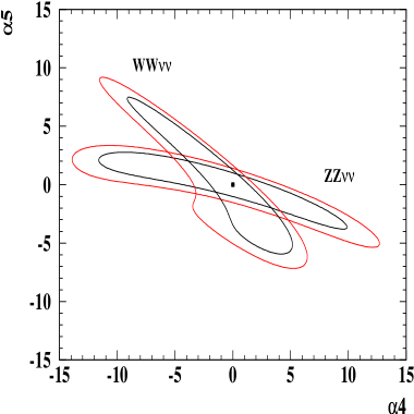
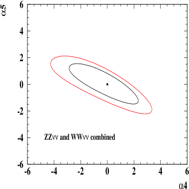
| , , | ||
| … | … | |
| … | … | |
| 2.3 TeV | 2.7 TeV | |
| 3.1 TeV | 3.7 TeV | |
The experimental sensitivity of an experiment at TESLA to the conserving parameters has been estimated from a likelihood fit to the angular distributions of the gauge boson production angles and the angles of the decay fermions in the channel, after detector simulation (using SIMDET V1.3 [36]) and event selection [32]. The results are summarised in Fig. 3 and Table 2. The separation and background suppression in hadronic final states use cuts on transverse momenta and recoil masses, utilising the excellent energy resolution and hermiticity, including the forward region, of the proposed TESLA detector. Three to four years of operation will cover up to the EWSB scale
The exotic channel can be accessed by operating TESLA in the mode. The different angular distributions in this channel allow a further reduction of correlations among conserving interactions. In particular, there can be no contaminations from a violating sector in this channel [31].
In the Standard Model with a very heavy Higgs, two loop diagrams create a sizeable contribution to the parameter , while the contributions to the other parameters remain small [38]. Using [38], the limits on from the two-dimensional fit in Table 2 translate to a Higgs mass of , demonstrating that virtual effects of an extremely heavy Higgs can be observed in vector boson scattering at a TESLA experiment.
| LHC | TESLA 800 GeV | |
| … | … | |
| … | … | |
| 2.3 TeV | 2.9 TeV | |
| 2.8 TeV | 4.9 TeV |
The one dimensional 68% C.L. limits from at LHC [37] are compared with the analogous prediction for a TESLA experiment in Table 3. Even though all backgrounds are included in the simulation of a TESLA experiment, TESLA exceeds the physics reach of LHC for QGCs and reaches the strong EWSB benchmark (3). As anticipated above, the limits for the QGCs are sligthly worse than the limits for the TGCs. As in the case of TGCs, no unitarisation prescriptions are required.
In summary, it has been demonstrated with realistic simulations that a TESLA experiment can probe the invariant and linearly breaking parameters of a strong EWSB sector exhaustively in the threshold region of strong interactions up to the EWSB scale .
2 Vector resonances and Pseudo-Goldstone bosons
If the EWSB sector includes a resonance below the EWSB scale, the vector boson pair production amplitude is unitarised by a Omnès rescattering factor
| (10) |
with one contribution reproducing the low energy theorem for Goldstone boson scattering at threshold far below any resonance and a second contribution from a resonance . A phenomenological study [39] shows that of production at a 800 GeV TESLA is competitive with at LHC, as shown in Fig. 4. The exclusion limit for LET (also excluding any resonance) at TESLA assumes perfect charm tagging, which is a realistic approximation for the proposed TESLA detector. Without any charm tagging, the significance is reduced to .

| TESLA | LHC | ||
| 800 GeV | |||
| LET | — | ||
| 2.5 TeV | — | — | |
| 1.6 TeV | |||
An example of a concrete model for the EWSB sector without a Higgs particle is the BESS model [40], which includes most technicolour models. The model assumes a triplet of new vector resonances , similar to the or techni-. These vector bosons mix with the electroweak gauge bosons and the mixing angle is proportional to the ratio , where is the self-coupling of the . The coupling of the to fermions is determined by a second parameter . The so called degenerate BESS model [41] is a special case, in which axial and vector resonances are almost degenerate in mass. Models for dynamical EWSB typically predict many pseudo Nambu-Goldstone bosons (PNGBs) from the breaking of a large global symmetry group and the lightest neutral PNGB calls for special attention.

The -channel is the preferred channel for the discovery of the vector resonances of the general BESS model, while the -channel is preferred for the degenerate BESS model [41]. The analysis in the fermionic channels is based on the observables , , , and (all with ). In the channel, the observables , and the longitudinally and transversely polarised differential cross sections and asymmetries have been used. The expected bounds from a TESLA experiment for the BESS model, obtained by combining all the observables, are shown in Fig. 5. In particular at large mixing, the sensitivity of a TESLA experiment is much higher than the combination of current electroweak data and expected LHC results.
In the case of the degenerate BESS, the LHC has the better discovery potential. However, if a neutral resonance with a mass below 1 TeV were discovered at the LHC, a TESLA experiment could study it in detail and attempt to split the two nearly degenerate resonances and measure their widths [42].

The best mode for production at TESLA is . Results for the significance , in the various tagged channels, for a technicolour model with and integrated luminosity at , are plotted in Fig. 6 [43]. Also shown is the significance that can be achieved with the optimal combination of the , , and channels. A strong signal is visible for all but . From the scaling law , one sees that a discovery would be possible for for near 35 GeV. Unlike the LHC, for high enough luminosities, a TESLA experiment can probe quite low values of and could measure ratios of a number of interesting decay modes. In the scenario of Fig. 6 and in the case of , an accuracy of could be achieved for the product .

The option at an collider is actually a more robust tool for discovering the than the collision mode. For and using a setup with a broad spectrum, a signal should be easily detectable in for masses up to 70% of the CMS energy with minimal luminosity () and a reasonably accurate measurement of would be obtained, as illustrated in Fig. 7.
Note that the discovery mode is strongest at larger , i. e. where becomes less robust. Once is known, the collision setup can be configured to yield a luminosity distribution that is strongly peaked at and, for much of the mass range of GeV, a measurement of can be made with statistical accuracy in the range [43], which is competitive with the LHC accuracy for measuring .
4 Compositeness
As one among other physical scenarios, strongly interacting electroweak bosons at energies of order 1 TeV could be interpreted as a signal of composite substructures of these particles at a scale of cm. Moreover, the proliferation of quarks and leptons could be taken as evidence for possible substructures of the matter particles [44]. In this picture, masses and mixing angles are a consequence of the interactions between a small number of elementary constituents – in perfect analogy to the quark/gluon picture of hadrons. No theoretical formalism has been set up so far which would reconcile, in a satisfactory manner, the small masses in the Standard Model with the tiny radii of these particles which imply very large kinetic energies of the constituents. However, the lack of theoretical formalism does not invalidate the physical picture or its motivation.
1 Contact interactions
In this agnostic approach, stringent bounds have been derived from high energy scattering experiments on possible non-zero radii of leptons, quarks and gauge bosons from decay data [45] and Bhabha scattering [46] in collisions, as well as from electron-quark and quark-quark scattering at HERA [47] and the Tevatron [48], respectively. From these analyses the compositeness scale has been bounded to less than cm.
Fermion pair production at high energies provides a very powerful instrument to set limits on fermion compositeness. This problem has been studied, based on four-fermion contact interactions which can be generated by the exchange of subconstituents [49]:
| (1) |
The strength of the interaction has been set to . The (inverse) contact scales can be identified, within an uncertainty of a factor of order 3, with the radius of the fermions. Detailed experimental simulations have shown that fermion pair production at TESLA provides a larger sensitivity to compositeness scales than the LHC, which reaches sensitivities up to about 20–35 TeV [50]. The high polarization that can be achieved for and beams, gives the TESLA collider another advantage. At c.m. energies of 500 GeV, the bounds on fermion compositeness are presented in Fig. 1 for the production of hadrons and muon pairs for an integrated luminosity of ab-1 [19] (see also [51, 52]). For muon pair production the significant effect of positron polarization [14] is also shown. The dependence on the sign of the interference term between composite and SM contributions is negligible in muon pair production, and only the average of and is presented in Fig. 1. Increasing the c.m. energy to 800 GeVresults in an increase of the sensitivities to and by about 30% [19].
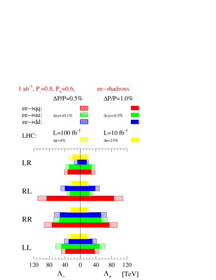
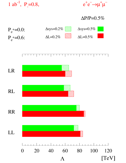
2 Leptoquarks
A very exciting prediction of fermion compositeness is the existence of leptoquarks [53]. They are novel bound states of subconstituents which build up leptons and quarks in this scenario. While the size of the couplings to and bosons follows from the electroweak symmetries, the Yukawa couplings to leptons and quarks are bound by experiment [54]. In the interesting mass range, these Yukawa couplings are expected to be weak. Currently leptoquark masses below about 250, 200 and 100 GeV are excluded for 1st, 2nd and 3rd generation leptoquarks [55].
These particles can also occur in grand unified theories. Moreover, in supersymmetric theories in which the parity is broken, squarks may be coupled to quarks and leptons, giving rise to production mechanisms and decay signatures analogous to leptoquarks. However, whereas leptoquarks sui generis disintegrate solely to leptons and quarks, a wide variety of decay modes is in general expected for squarks, including the large ensemble of standard supersymmetric decay channels, see e.g. [56]. Since leptoquark bound states in the compositeness picture build up a tower of states with non-zero spins, the phenomenology of the two scenarios is clearly distinct.
Leptoquarks can exist in a large variety of states carrying or quantum numbers and being scalar or vectorial in the simplest representations [57]. They can be produced in collisions pairwise, , through –channel exchange and partly through –channel exchange [58, 59]. The particles decay to a charged lepton, or a neutrino, and a jet, giving rise to visible (a) , (b) , and (c) final states. Since leptoquarks generate a peak in the invariant () mass, they are easy to detect in the cases (a) and (b) up to mass values close to the kinematical limit [60].
Since leptoquarks carry color, they are produced copiously [61] in hadron collisions through the subprocesses and . Leptoquarks can therefore be generated at the LHC with masses up to about 1.5 TeV [62]. Experiments at colliders are nevertheless important to identify the electroweak properties of these novel states. Taking into account statistical errors for leptoquark pair production, their electroweak couplings to and can be measured at the level of [63]. Combining the processes and [with brems- and beamstrahlung photons], the Yukawa couplings can be determined with an accuracy of , as can be inferred from Table 1 [64].
| TESLA | LHC | current | TESLA | LHC | current | |
|---|---|---|---|---|---|---|
| 330 GeV | ||||||
| 350 GeV | ||||||
| 370 GeV | ||||||
| 390 GeV | ||||||
For leptoquark masses beyond the kinematical limit TESLA can study virtual leptoquark effects in fermion pair production processes . Assuming Yukawa couplings of electromagnetic strength, TESLA will be sensitive to scalar leptoquark masses of TeV for GeV at high luminosities including electron (positron) polarization of 80% (60%) [19], thus extending the reach of the LHC significantly.
5 Conclusions
TESLA provides a rich environment for precision tests of theories beyond the SM. In general the reach in the masses of new particles that can be found at LHC will be comparable or larger than at TESLA. However, TESLA can measure the couplings and properties of the novel particles with high accuracy contrary to the LHC, thus supporting the complementarity of both colliders.
A major class of extensions beyond the SM consists of adding extra dimensions to the conventional Minkowski space, which may turn out to be large with string scales in the TeV range. The LHC will be sensitive to Kaluza–Klein-graviton emission up to scales TeV , which denotes the fundamental Planck scale in the higher dimensional space. While the reach of TESLA is comparable to the LHC, TESLA will be able to disentangle the scale and the number of extra dimensions from the energy dependence of the graviton emission cross section unambiguously in contrast to the LHC. Moreover, TESLA can probe scales up to TeV via virtual effects due to KK exchange, leading effectively to fermionic contact interactions. The angular distributions of fermion pair production processes can be used to show that the virtual KK states carry spin 2.
If Higgs bosons do not exist, the onset of strong interactions will become visible at high energies. TESLA will probe the threshold region for strong interactions up to the cut-off scale TeV , which defines the scale of strong electroweak symmetry breaking in this scenario. The TESLA sensitivity exceeds the LHC sensitivity. Moreover, the couplings of novel strong vector resonances and pseudo Nambu-Goldstone bosons can be determined much more accurately than at the LHC.
In the framework of conventional compositeness theories TESLA will exceed the sensitivity to the compositeness scales significantly compared to the LHC. In addition TESLA will allow an accurate measurement of leptoquark electroweak and Yukawa couplings, when leptoquarks will have been discovered at the LHC in the accessible mass range. However, if the leptoquark masses turn out to be too large for direct production, TESLA can extend the mass reach indirectly by means of virtual leptoquark exchange in fermion pair production.
The comparison between TESLA and the LHC is summarized in Table 1, which clearly confirms the complementarity of these two colliders.
| Alternative | TESLA | LHC |
| graviton radiation | TeV | TeV |
| graviton exchange | TeV | ? |
| strong interactions | (3 TeV) | |
| vector resonance couplings | ||
| Goldstone couplings | (1%) | (10%) |
| leptoquark Yukawa couplings | upper bounds | |
| compositeness scale | TeV | TeV |
References
-
[1]
N. Arkani-Hamed, S. Dimopoulos, G. Dvali.
Phys. Lett. B429:263, 1998;
N. Arkani-Hamed, S. Dimopoulos, G. Dvali. Phys. Rev. D59:086004, 1999;
I. Antoniadis, N. Arkani-Hamed, S. Dimopoulos, G. Dvali. Phys. Lett. B436:257, 1998. -
[2]
I. Antoniadis.
Phys. Lett. B246:377, 1990;
I. Antoniadis, C. Munoz, M. Quiros. Nucl. Phys. B397:515, 1993;
I. Antoniadis, K. Benakli. Phys. Lett. B326:69, 1994;
I. Antoniadis, K. Benakli, M. Quiros. Phys. Lett. B331:313, 1994. -
[3]
L. Randall, R. Sundrum.
Phys. Rev. Lett. 83:3370, 1999,
Phys. Rev. Lett. 83:4690, 1999. - [4] N. Seiberg, E. Witten. JHEP 9909:032, 1999.
- [5] J.J. van der Bij. Int. J. Phys. 1:63, 1995
- [6] C.D. Hoyle et al. Sub–millimeter tests of the gravitational inverse–square law: A search for “large” extra dimension. hep-ph/0011014.
- [7] G.F. Giudice, R. Rattazzi, J.D. Wells. Nucl. Phys. B544:3, 1999.
-
[8]
S. Cullen, M. Perelstein.
Phys. Rev. Lett. 83:268, 1999;
L. Hall and D. Smith. Phys. Rev. D60:085008, 1999;
V. Barger, T. Han, C. Kao, R.J. Zhang. Phys. Lett. B461:34, 1999;
C. Hanhart, D.R. Phillips, S. Reddy, M.J. Savage. Nucl. Phys. B595:335–359, 2001. - [9] T. Han, J. Lykken, R.J. Zhang. Phys. Rev. D59:105006, 1999.
-
[10]
E.A. Mirabelli, M. Perelstein, M. Peskin.
Phys. Rev. Lett. 82:2236, 1999;
K. Cheung, W.Y. Keung. Phys. Rev. D60:112003, 1999. - [11] G.W. Wilson. Study of the sensitivity to extra–dimensions in the photon–graviton channel with polarised beams. LC-PHSM-2001-010. http://www.desy.de/~lcnotes
- [12] A. Vest. Search for extra dimensions in graviton emission . LC-TH-2000-058. http://www.desy.de/~lcnotes
- [13] G. Montagna, M. Moretti, F. Piccinini, O. Nicrosini. Nucl. Phys. B541:31, 1999.
- [14] G. Moortgat-Pick, H. Steiner. Beam polarization at a Linear Collider : What do we gain with positron polarization. LC-TH-2000-055. http://www.desy.de/~lcnotes
- [15] L. Vacavant, I. Hinchliffe. Model Independent Extra-dimension signatures with ATLAS. ATL-PHYS-2000-016, hep-ex/0005033.
- [16] K. Cheung, W.-Y. Keung. Phys. Rev. D60:112003, 1999.
- [17] D. Atwood, S. Bar-Shalom, A. Soni. Phys. Rev. D61:116011, 2000.
-
[18]
J.L. Hewett.
Phys. Rev. Lett. 82:4765, 1999;
T.G. Rizzo. Phys. Rev. D59:115010, 1999. - [19] S. Riemann. Fermion–pair production at a Linear Collider - A sensitive tool for new physics searches Proceedings of 5th International Linear Collider Workshop (LCWS2000), LC-TH-2001-007. http://www.desy.de/~lcnotes
- [20] T.G. Rizzo. Phys. Rev. D60:115010, 1999.
-
[21]
I. Antoniadis, K. Benakli, M. Quiros.
Phys. Lett. B460:176, 1999;
P. Nath, Y. Yamada, M. Yamaguchi. Phys. Lett. B466:100, 1999. -
[22]
W.D. Goldberger, M.B. Wise.
Phys. Rev. Lett. 83:4922, 1999;
O. DeWolfe, D.Z. Freedman, S.S. Gubser, A. Karch. Phys. Rev. DD62:046008, 2000;
M.A. Luty, R. Sundrum. Phys. Rev. D62:035008, 2000. - [23] H. Davoudiasl, J.L. Hewett, T.G. Rizzo. Phys. Rev. Lett. 84:2080, 2000.
-
[24]
H. Davoudiasl, J.L. Hewett, T.G. Rizzo.
Phys. Lett. B473:43, 2000,
hep-ph/0006041,
Phys. Lett. B493:135–141, 2000;
A. Pomarol. Phys. Lett. B486:153, 2000;
Y. Grossman, M. Neubert. Nucl. Phys. B474:361, 2000;
R. Kitano. Phys. Lett. B481:39, 2000;
S. Chang et al. Phys. Rev. D62:084025, 2000;
T. Ghergetta, A. Pomarol. Nucl. Phys. B586:141, 2000. - [25] J.L. Hewett, F. Petriello, T.G. Rizzo. Signals for non–commutative interactions at linear Colliders. hep-ph/0010354.
-
[26]
T. Appelquist, C. Bernard.
Phys. Rev. D22:200, 1980;
A.C. Longhitano. Phys. Rev. D22:1166, 1980;
A.C. Longhitano. Nucl. Phys. B188:118, 1981;
T. Appelquist, G. Wu. Phys. Rev. D51:240, 1995, hep-ph/9406416. -
[27]
S. Dawson, G. Valencia.
Nucl. Phys. B439:3, 1995,
hep-ph/9410364;
A. Brunstein, O.J. Eboli, M.C. Gonzalez-Garcia. Phys. Lett. B375:233, 1996, hep-ph/9602264;
J.J. van der Bij. Phys. Rev. D35:1088, 1987;
J.J. van der Bij. Phys. Lett. B296:239, 1992;
J.J. van der Bij, B. Kastening. Phys. Rev. D57:2903, 1998, hep-ph/9708438. -
[28]
S. Weinberg.
Physica A96:327, 1979;
A. Manohar, H. Georgi. Nucl. Phys. B234:189, 1984;
H. Georgi, L. Randall. Nucl. Phys. B276:241, 1986. - [29] K. Hagiwara, R.D. Peccei, D. Zeppenfeld, K. Hikasa, Nucl. Phys. B282:253, 1987.
- [30] W. Menges. A Study of charged current triple gauge couplings at TESLA. LC-PHSM-2001-022.
-
[31]
E. Boos, H.J. He, W. Kilian, A. Pukhov, C.P. Yuan, P.M. Zerwas.
Phys. Rev. D61:077901, 2000,
hep-ph/9908409;
Phys. Rev. D57:1553, 1998, hep-ph/9708310. - [32] R. Chierici, S. Rosati, M. Kobel. Strong electroweak symmetry breaking signals in WW scattering at TESLA. LC-PHSM-2001-038.
- [33] W. Kilian. WHIZARD 1.0: A generic Monte-Carlo integration and event generation package for multi-particle processes. http://www-ttp.physik.uni-karlsruhe.de/Progdata/whizard/. LC-TOOL-2001-039.
- [34] T. Ohl, Comput. Phys. Commun. 120:13, 1999, hep-ph/9806432.
-
[35]
T. Ohl.
O’Mega: An optimizing matrix element generator.
Proceedings of 7th International Workshop on Advanced Computing and Analysis
Techniques in Physics Research (ACAT 2000),
hep-ph/0011243;
T. Ohl. O’mega and WHIZARD: Monte Carlo event generator generation for future colliders. Proceedings of 5th International Linear Collider Workshop (LCWS 2000), hep-ph/0011287;
M. Moretti, T. Ohl, J. Reuter. O’Mega: An Optimizing Matrix Element Generator. http://heplix.ikp.physik.tu-darmstadt.de/~ohl/omega/, LC-TOOL-2001-040. - [36] M. Pohl, H.J. Schreiber. SIMDET Version 3 – A parametric Monte Carlo for a TESLA detector. DESY 99-030.
-
[37]
A.S. Belyaev, O.J. Eboli, M.C. Gonzalez-Garcia, J.K. Mizukoshi,
S.F. Novaes and I. Zacharov.
Phys. Rev. D59:015022, 1999, hep-ph/9805229;
S. Haywood et al. Electroweak physics. hep-ph/0003275. -
[38]
J.J. van der Bij,
Nucl. Phys. B255:648, 1985;
V. Borodulin and G. Jikia. Nucl. Phys. B520:31, 1998, hep-ph/9712419. - [39] T. Barklow. LET signals in at GeV. Proceedings of 5th International Linear Collider Workshop (LCWS 2000).
- [40] R. Casalbuoni, S. De Curtis, D. Dominici and R. Gatto. Nucl. Phys. B282:235, 1987.
-
[41]
R. Casalbuoni, A. Deandrea, S. De Curtis, D. Dominici, F. Feruglio, R. Gatto
and M. Grazzini.
Phys. Lett. B349:533, 1995, hep-ph/9502247 ;
R. Casalbuoni, A. Deandrea, S. De Curtis, D. Dominici, R. Gatto and M. Grazzini. Phys. Rev. D53:5201, 1996, hep-ph/9510431. - [42] R. Casalbuoni, A. Deandrea, S. De Curtis, D. Dominici, R. Gato and J.F. Gunion. JHEP 9908:11, 1999, hep-ph/9904268.
- [43] R. Casalbuoni, A. Deandrea, S. De Curtis, D. Dominici, R. Gatto and J.F. Gunion. Nucl. Phys. B555:3, 1999, hep-ph/9809523.
-
[44]
H. Harari.
Proceedings, 1984 Scott. Summer School (St. Andrews);
M.E. Peskin. Proceedings of Int. Symp. on Lepton and Photon Interactions at High Energies, eds. M. Konuma and K. Takahashi (Kyoto 1985); W. Buchmüller. Acta Phys. Austr. Suppl. 27:517, 1985. - [45] G. Köpp, D. Schaile, M. Spira, P.M. Zerwas. Z. Phys. C65:545, 1995.
-
[46]
H. Kroha.
Phys. Rev. D46:58, 1992;
G. Alexander et al. Test of the four–fermion contact interaction in collisions at 130–140 GeV. CERN-PPE 96-098. - [47] S. Aid et al. Phys. Lett. B353:578, 1995.
- [48] F. Abe et al. Phys. Rev. Lett. 75:608, 1995.
- [49] E. Eichten, K.D. Lane, M.E. Peskin. Phys. Rev. Lett. 50:811, 1983.
- [50] S. Jain, A.K. Gupta, N.K. Mondal. Phys. Rev. D62:095003, 2000.
- [51] S. Riemann. Sensitivity of fermion pair production to new physics phenomena. Proceedings LCWS 1999, ISBN 84-490-1977-X.
- [52] A.A Babich, P. Osland, A.A. Pankov, N. Paver. Contact interactions and polarized beams at a Linear Collider. LC-TH-2001-021, hep-ph/0101150. http://www.desy.de/~lcnotes
- [53] See e.g. J.L. Hewett, T.G. Rizzo. Phys. Rept. 183:193, 1989.
-
[54]
J. Kalinowski, R. Rückl, H. Spiesberger, P.M. Zerwas.
Z. Phys. C74:595, 1997;
J. Blümlein. Z. Phys. C74:605, 1997;
A.F. Żarnecki. Eur. Phys. J. C17:695, 2000. - [55] CDF and D0 Collaborations (D.E. Acosta for the collaborations). Leptoquark searches at the TEVATRON. FERMILAB-CONF-00-132-E and references therein.
- [56] E. Perez, Y. Sirois, H. Dreiner. Proceedings, Future Physics at HERA, eds. G. Ingelman, A. DeRoeck and R. Klanner, DESY 1996.
- [57] W. Buchmüller, R. Rückl, D. Wyler. Phys. Lett. B191:442, 1987.
-
[58]
D. Schaile, P.M. Zerwas.
Proceedings, Physics at Future Accelerators, ed. J.H. Mulvey (La Thuile and
Geneva 1987).
CERN 87-07;
A. Djouadi, M. Spira, P.M. Zerwas. Proceedings, Collisions at 500 GeV: The Physics Potential, Munich–Annecy–Hamburg 1991/93, ed. P.M. Zerwas. DESY 92-123B. -
[59]
J. Blümlein, R. Rückl.
Phys. Lett. B304:337, 1993;
J. Blümlein, E. Boos. Nucl. Phys. Proc. Suppl. B37:181, 1994;
J. Blümlein, E. Boos, A. Kryukov. Phys. Lett. B392:150, 1997. - [60] R. Rückl, R. Settles, H. Spiesberger. In: Conceptual Design report of a 500 GeV Linear Collider with Integrated X–ray Laser Facility, chapter 1.8.3. DESY 1997-048.
-
[61]
J. Hewett, S. Pakvasa.
Phys. Rev. D37:3165, 1988;
O.J.P. Éboli, A.V. Olinto. Phys. Rev. D38:3461, 1988;
M. Krämer, T. Plehn, M. Spira, P.M. Zerwas. Phys. Rev. Lett. 79:341, 1997;
J. Blümlein, E. Boos, A. Kryukov. Z. Phys. C76:137, 1997. - [62] S. Abdullin, F. Charles. Phys. Lett. B464:223, 1999.
- [63] J. Blümlein. Precision of electro–weak couplings of scalar leptoquarks at TESLA. LC-TH-2000-050, hep-ph/0009323. http://www.desy.de/~lcnotes
- [64] A.F. Żarnecki. Measurement of the leptoquark Yukawa couplings in collisions at TESLA. LC-PHSM-2001-020.
Chapter 4 Precision Measurements
1 Electroweak Gauge Bosons
The measurement of gauge boson properties has in the past strongly influenced our knowledge of electroweak interactions. The primary goal is to establish the non-Abelian nature of electroweak interactions. With very precise measurements one can constrain new physics at scales above the direct reach of the machine through loop effects. Alternatively, small effects from operators in an effective Lagrangian, that are suppressed by , can be measured, where is the scale where new physics sets in. Also for the extrapolation of couplings to high scales, to test theories of grand unification, very high precision is needed. At TESLA there are mainly two ways to study properties of W- and Z-bosons:
-
•
One can study the couplings amongst gauge bosons. These couplings are especially sensitive to models of strong electroweak symmetry breaking and are most precisely measured at the highest possible energies.
-
•
The masses and couplings of the W and Z, especially the effective weak mixing angle in Z decays, , can be measured, similar to LEP and SLC, however with much higher luminosity and polarised beams.
In addition, an improved measurement of the couplings of the electroweak gauge bosons to quarks will provide further insight into the flavour physics of the CKM-matrix. The experimental methods are complementary to the b-factories and hadron colliders and can provide independent consistency checks.
1 W-production at high energies
At high energies W bosons are produced either in pairs, , or singly via . W-pair production falls, far above threshold, like while single W-production rises logarithmically with the energy. At TESLA-energies both cross sections are of about the same size.
The Feynman diagrams for on-shell W-pair production are shown in Fig. 1. Due to the nature of the charged current couplings, the contribution of the -channel -exchange diagram vanishes for right-handed electrons or left-handed positrons. Therefore it can be switched off completely by polarising one of the beams appropriately. Its contribution can also be enhanced by a factor two or four by polarising one or both beams in the opposite way. For energies that are much higher than the weak boson-masses, the combined Z and exchange can be replaced by the neutral member of the W weak isospin triplet, because the orthogonal combination corresponding to the weak hypercharge boson does not couple to the . Therefore the coupling to the electrons and positrons is also purely at high energies. Already at TESLA energies, the cross section for right-handed electrons is suppressed by at least a factor of ten relative to left-handed electrons for all polar angles.

Single W production is dominated by photon-W fusion (see Fig. 2). Since the helicity only matters for the beam that radiates the W, varying the electron polarisation can switch off or double single production while varying the positron polarisation affects single production in the same way.

Figure 3 a) shows the total cross section as a function of the centre of mass energy for both processes and Fig. 3 b) the differential cross section for W-pair production for the two electron helicities at .
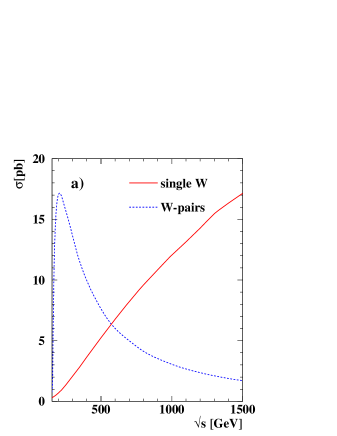
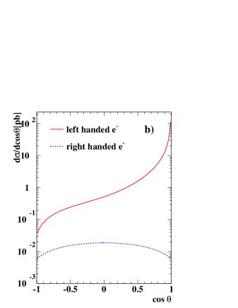
In addition, at a - and e-collider the processes and are accessible. The first process proceeds via W-exchange in the -channel while the second one involves the vertex shown in Fig. 2. The cross sections for these two processes are large ( for and for e at ), however they occur predominantly at a lower scale.
All processes are sensitive to the triple gauge couplings , , which are conventionally parameterised as [3]
| (1) | |||||
using the antisymmetric combinations and their duals . The overall coefficients are and with being the weak mixing angle. With the couplings as momentum dependent form factors, eq. (1) parameterises the most general vertex, that couples three vector bosons. In a systematic analysis the coefficients of the triple gauge couplings in eq. (1) are related to the coefficients of an effective Lagrangian and the latter can be inferred from measurements of the former. Keeping only the lowest orders (dimension four and six) of a systematic expansion in the energy, constant values for the coupling arise. If the terms in the effective Lagrangian are properly organised according to their gauge transformation properties, triple couplings will in general be related to quartic couplings.
Electromagnetic gauge invariance requires that and at zero momentum transfer. In the Standard Model one has , all other couplings are equal to zero.
Amongst the different couplings and are C- and P-conserving, is C and P-violating, but CP-conserving while violate CP.
While single W production is basically sensitive to WW couplings only, W pair production always involves a mixture of WW and WWZ couplings. However, as it is demonstrated in Fig. 4, the two types of couplings can be disentangled with the help of beam polarisation.
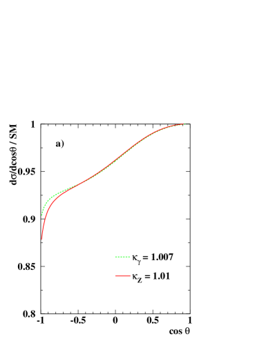
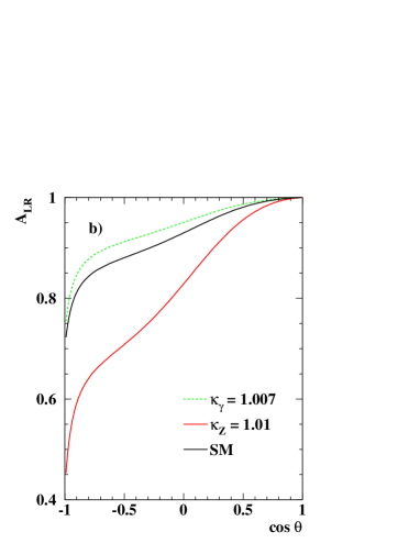
For the analysis of triple gauge couplings in W-pair production in principle five different observables are available:
-
•
the polar angle of the outgoing with respect to the incoming direction, ;
-
•
the polar angle of the fermion with respect to the W flight direction in the W rest frame for both W-bosons, , this variable is sensitive to the longitudinal polarisation of the W;
-
•
the azimuthal angle of the fermion in the W-beam plane for both Ws, , sensitive to the transverse polarisation.
Not all of the above variables can be determined unambiguously in all decays. For about 44% of the W-pairs one W decays leptonically and the other one into two jets. In these events the polar angle can be reconstructed from the jet momenta and the lepton charge. The decay angles of the leptonically decaying W can be reconstructed without ambiguity and for the hadronically decaying W, since the quark and the antiquark cannot be distinguished, with the ambiguity . This event sample has the by far highest sensitivity to gauge boson couplings. 46% of the W-pairs decay into four jets. If the correct jet pairing is found one still has the sign ambiguity for the decay angles of both W bosons plus, since the W-charges cannot be determined, the ambiguity for the production angle, so that these events add only little to the sensitivity. The remaining 11% decay fully leptonically. In about half of them one lepton is a , so that because of the additional neutrinos, too little information is available. For the other half all information can be calculated with a twofold ambiguity. However the additional statistics from these events is so small that the analysis of the mixed decays alone gives a good estimate of the total sensitivity.
Since it is inconvenient to work with five independent variables, always some variable reduction is used. For the TESLA studies the spin density matrix has been applied which obtains close to optimal results [4].
At TESLA mixed decays of W-pairs can be selected with very high efficiency and low background. The large forward peak, that is partially lost in the beampipe, is dominated by -channel neutrino exchange and is thus not sensitive to anomalous couplings (see Fig. 4). Due to the large boost, the W-production angle can be measured with significantly higher accuracy than at LEP. Also the resolution of the W-decay angles is good enough that detector effects can be almost neglected.
In the spin density formalism the signals from the C,P,CP-violating couplings are clearly separated from the C,P-conserving ones. For example the imaginary parts of the off-diagonal elements of the spin-density matrix are non-zero only if CP-violating couplings are present. Because of the negligible correlations between the different sets of couplings the fits can be done separately.
 |
 |
 |
 |
Although with beam polarisation all five C,P-conserving couplings can be determined simultaneously, to test certain models it is still useful to perform single parameter fits with all other couplings fixed to the values predicted by the Standard Model. In these fits it is also reasonable to impose the relations amongst the parameters suggested by invariance [5]:
Table 1 shows the results of the different single parameter fits including the C or P violating couplings for at and at . For both cases an electron polarisation of 80% and a positron polarisation of 60% is assumed. Figure 5 shows the results of the five-parameter fit for . Only the combinations with large correlations are shown.
| coupling | error | |
|---|---|---|
| C,P-conserving, relations: | ||
| C,P-conserving, no relations: | ||
| not C or P conserving: | ||
Systematic uncertainties from detector effects, backgrounds and beamstrahlung are small. The beam polarisation can be determined from a Blondel scheme [6, 7], so that no additional systematics enter. If only electron polarisation is available the statistical errors increase by roughly 50%. However, since the forward peak in the cross section is completely dominated by the neutrino -channel exchange, which is present for left handed electrons only, also in this case the beam polarisation can be determined from the data alone [7].
The radiative corrections need to be known significantly better than 1%. Using the double-pole approximation, the cross section for W-pair production can currently be predicted to better than 0.5% away from the threshold region up to 500 GeVwith RaccoonWW [8] and YFSWW3 [2]. Above large double logarithmic corrections (electroweak Sudakov logarithms) arise from the virtual exchange of soft and collinear gauge bosons. These corrections are numerically important, but they have been studied extensively and are theoretically under control [9].
In general the total errors on the anomalous couplings are . Loop corrections to the couplings are expected to be of order , one order of magnitude larger than the expected precision. For the case of Supersymmetry it has been shown that the loop corrections are indeed of that size [10, 11] and should thus be visible at TESLA.
Figure 6 compares the obtainable precision of and at the different machines. Especially for , where, because of the lower dimension of the corresponding operator, experiments are sensitive at a lower energy to potential new physics at a high scale, TESLA has a much higher sensitivity than LHC.
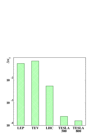
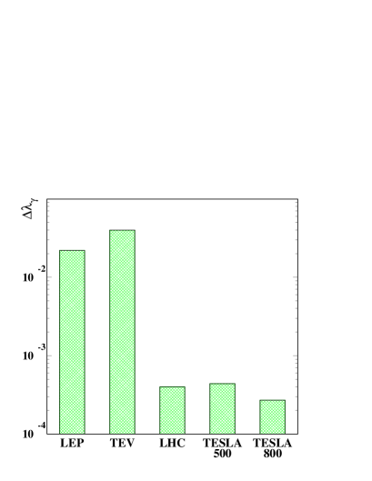
For the additional processes, and , at the - and e-collider only theoretical studies with low luminosity exist [12]. An extrapolation to the presently expected luminosity still yields errors that are an order of magnitude worse than the ones expected from W-pair production in . However, these studies use only the total cross section in the central region of the detector and additional sensitivity can be expected from a detailed analysis of the angular dependence and the W-polarisation. With the same simplifications the expectations for single W production in collisions are slightly worse than for the - and e-collider.
In addition to single and pair production of gauge bosons also triple gauge boson production will be visible at TESLA. The cross sections are, in the heavy Higgs limit, for WWZ and for ZZZ [13, 14]. Both processes have their maximum cross section between 500 and 1000 GeV. Requiring a photon of more than 20 GeV energy at a polar angle above the total cross section for ZZ is of the order and for WW about . Using the latter two channels the anomalous couplings and which modify the -vertex but not the triple-gauge-couplings can be measured to the 0.2 level with , an integrated luminosity of and polarised beams, corresponding to in the operators and [15, 14].
Also these measurements require adequate theoretical calculations. The present status is summarised in [16].
2 High precision measurements at lower energies
With a luminosity of at energies close to the Z-pole TESLA can produce Z-bosons in about 50-100 days of running. A similar luminosity is possible close to the W-pair threshold. In this scenario, referred to as GigaZ in the following, the measurements already performed at LEP and SLC can be redone with increased precision.
Measurement of the weak mixing angle
One of the most sensitive quantities to loop corrections from the Higgs-boson is the effective weak mixing angle in Z-decays . The most sensitive observable to is the left-right asymmetry
where is the total cross section for left/right-handed polarised electrons and the longitudinal electron polarisation. For pure Z-exchange is then given by , being the vector- (axial-vector-) coupling of the Z to the electron and . can be measured during GigaZ running from hadronic Z-decays with very high efficiency and low background. Details on the measurement of and the other observables can be found in [17]. The statistical error with events will be of the order which has to be matched by systematics. The polarisation needs to be known to . This is only possible if polarised electrons and positrons are available, so that the polarisation can be measured directly from data using the Blondel-scheme [6]. The cross section for an electron polarisation and a positron polarisation is given by
| (2) |
where is the cross section for unpolarised beams.
If all four combinations of beam helicities are measured can be obtained independently from an external polarisation measurement:
| (3) |
where in denotes the sign of the electron- and the sign of the positron polarisation.
This formula assumes, however, that the absolute polarisation values of the bunches with opposing helicity states are equal. To assure this, or to get the relevant corrections, polarimeters are still needed. Since only relative measurements within one beam are needed most systematics cancel, so that with this scheme the polarisation can be measured with the required accuracy. To obtain optimal statistical precision only one tenth of of the luminosity needs to be spent on the small cross sections . For the statistical error using the Blondel scheme is only slightly larger than with an external polarisation measurement. For 20% positron polarisation and Zs the statistical error is .
Around the Z peak the change of with the beam energy is . The variation is due to the -Z interference, so that the difference of and needs to be known. Not to be dominated by the knowledge of the beam energy one needs a spectrometer with a precision of 1 MeV that can be calibrated relative to with a short scan around the Z-resonance. Also because of the energy dependence of , the amount of beamstrahlung expected for GigaZ running shifts by . The beamstrahlung thus needs to be understood to a few percent which seems possible [18]. If the same beamstrahlung as in the measurement is also present in the calibration scan the beamstrahl-shift is absorbed in an apparent shift of the centre of mass energy, so that in principle no corrections are necessary. Since all other systematic errors are small, is a realistic estimate of the final error. This corresponds to an error in the weak mixing angle of .
Due to the polarised beams and the excellent b-tagging also the measurements using the b-quark forward-backward asymmetry can be improved by roughly a factor 15 relative to LEP and SLC. GigaZ thus can clear up the slight discrepancy between the b-asymmetry at LEP and SLC and at SLC [19].
Measurements of the Z-partial widths
For the observables sensitive to the partial and total widths of the Z the situation is less spectacular. The measurement of the total Z-width will be dominated by the relative precision of the beam spectrometer. A total precision of is thus within reach (see Part IV-7.3).For the selection efficiencies for hadrons, muons and taus a factor three improvement relative to the best LEP experiment should be possible [20]. Also the experimental systematics on the luminosity might be improved, however, this would in addition require an improvement of the theoretical error, which is 0.05% at present.
The interesting physics parameters that can be derived from the lineshape parameters are
-
•
the mass of the Z ;
-
•
the strong coupling constant at the scale of the Z-mass ;
-
•
the radiative correction parameter, normalising the strength of the leptonic Z-couplings to the fermions [21];
-
•
the number of light neutrino species .
The possible improvements in these parameters are, together with the other observables at GigaZ, summarised in Table 2. The precision on all observables, obtained from the cross section around apart from itself can be improved by a factor two to three.
| LEP/SLC/Tev [19] | TESLA | |
| lineshape observables: | ||
| heavy flavours: | ||
Due to the extremely good b-tagging capabilities at TESLA, also the ratio of the Z partial width to to the hadronic width, , can be improved by a factor five relative to LEP.
Measurement of the W-mass
The W-mass can be obtained from a scan around the W-pair production threshold [22]. Near threshold the -channel production is suppressed by while the -channel is only suppressed by , where is the velocity of the W in units of . Due to the leading, -suppressed, contribution, a scan around the threshold has a high sensitivity to the W-mass. Also for the -channel only the well known We-coupling is involved, so that the total cross section can be predicted without uncertainties from new physics. Any anomalous triple gauge couplings enter via the -channel and are therefore suppressed by an additional factor . It is therefore possible to measure the W-mass precisely from a scan of the threshold region.
It should however be noted, that the double pole approximation is not valid in the threshold region. In order to reach sufficient accuracy in this energy range, a full four-fermion calculation with radiative corrections is required. The necessary improvements should be possible within the coming years such that the theoretical accuracy will be no obstacle to the precision tests.
With TESLA one can collect an integrated luminosity of per year at . The different polarisation states allow to enhance or suppress the signal helping to obtain the background directly from the data. A five point scan with and an additional point at has been simulated [22], assuming the same efficiency and purity as reached at LEP. With a total error of on the luminosity and on the selection efficiencies can be measured with a total precision of . The method is experimentally robust, for example even if the efficiencies are left free in the fit, the error only increases to . The achievable errors at the scan points are compared with the sensitivity to the W-mass in Fig. 7.
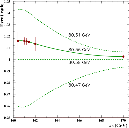
Interpretation of the high precision data
The high precision measurements can be used to test the Standard Model at the loop level. However one of the most important radiative corrections is due to the running of the electromagnetic coupling from zero momentum transfer to the Z-scale. This running is mainly caused by the contribution of fermion loops. The lepton loops can be calculated reliably without any significant uncertainty. However, due to additional QCD corrections the quark loops are much more uncertain. can be expressed as . If is calculated in a completely model independent fashion from a convolution of the cross section alone using only the optical theorem [23, 24], one obtains from the low energy data, including the latest BES results [25], corresponding to an uncertainty in the Standard Model prediction of of 0.00014. However, the sensitivity to the details of the resonance region can be reduced significantly, if the low energy data is used to fit the coefficients of a QCD operator product expansion instead of integrating the total cross section. If the hadronic cross section is known to 1% up to the -resonances the uncertainties are and [24].
A Z-mass error of 2 MeV from LEP contributes 0.000014 to the uncertainty of the prediction, about the same size as the experimental error and the uncertainty from . For the direct uncertainty due to is 2.5 MeV. However, if the beam energy is calibrated relative to the Z-mass, so that the relevant observable is , the error is smaller by a factor three.
An uncertainty in the top quark-mass of results in an uncertainty of the prediction of 0.00003 and in the one for of . For a top-mass error of , as it is possible from a top-threshold scan at TESLA (see section 3) this uncertainty is completely negligible.
Including the possible improvement on very stringent tests of the Standard Model are possible. Figure 8 shows as an example the variation of the fit- as a function of the Higgs-mass for the present data and for TESLA. It can be seen that the Higgs-mass can indirectly be constrained at the level of 5% [17, 26].
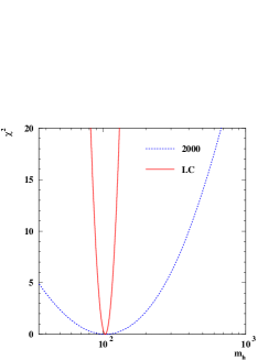
If the Higgs-mass is in the range predicted by the current precision data, the Higgs will have been found at the time of the high precision electroweak measurements. In this case the data can be used to check the consistency of the SM or to measure free parameters in by then established extensions of the model. As an example Fig. 9 shows the constraints that can be obtained in and from the low energy running if other SUSY parameters, especially the stop sector, are already known or, alternatively, in and if and the parameters, that can be measured from the light stop only, are known [26]. Further applications of GigaZ to Supersymmetry are discussed in chapter 2.
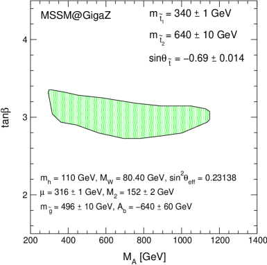 |
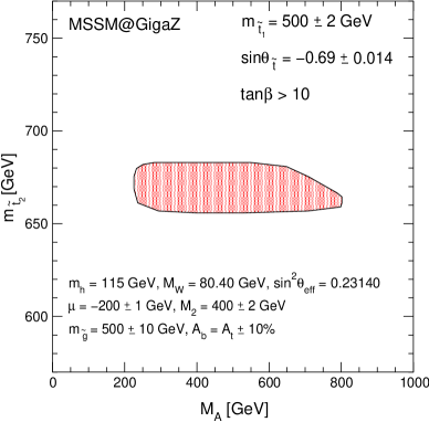 |
For more model independent analyses frequently reparameterisations of the radiative correction parameters are used where the large isospin-breaking corrections are absorbed into one parameter, so that the others depend only on the logarithmic terms. One example are the so called parameters [27]
In this parameterisation absorbs the large isospin-splitting corrections, contains only a logarithmic dependence while is almost constant in the Standard Model and most extensions. Figure 10 a)-c) shows the the expectations in the -planes, compared to present data and to the SM prediction. Since the prediction for is almost constant, in Fig. 10 d) the -plane is shown, if is fixed to the predicted value. In this case the precision along the large axis of the ellipse is dominated by the precise measurement of the W-mass.
In many extensions of the Standard Model can be varied freely by adjusting some masses, so that, with the new physics for every Higgs-mass up to a TeVthe prediction can be brought in agreement with the present data. This is also true to some extent with TESLA if the W-mass is not measured precisely. Only with the very accurate determination of , one can tightly constrain without the knowledge of .
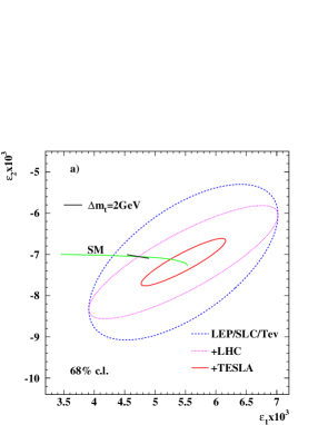 |
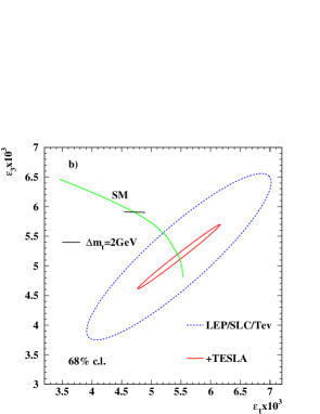 |
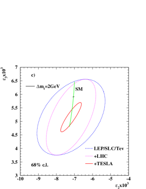 |
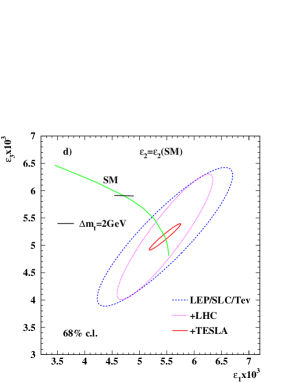 |
As an example of a possible interpretation of the precision data in the model independent framework, Fig. 11 shows the prediction of the 2 Higgs-doublet model (2HDM) for the ST parameters [28], which are basically equivalent to the parameters, for cases where a light Higgs exists but will not be seen directly (see section 3) compared to the present data and the projection of GigaZ [29]. Only with the precision of GigaZ it will be possible to distinguish between the Standard Model and the 2HDM.
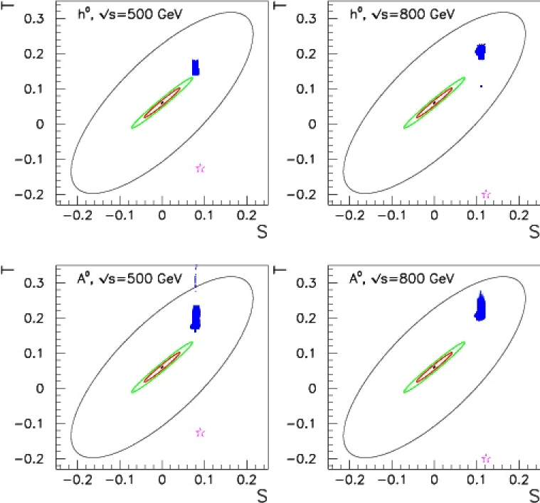
3 Measurements of CKM-matrix elements
TESLA can also contribute to the measurement of the CKM matrix in W decays. There are three ways how a linear collider can access these matrix elements:
-
•
in principle the absolute values of all elements not involving top-quarks can be measured in W-decays;
-
•
the elements involving b-quarks, including phases, can be accessed in B-decays with the GigaZ option;
-
•
the elements involving top quarks can be obtained from top decays.
The absolute values of the CKM elements can be obtained from the partial width of the W decaying into a specific quark final state. For this measurement both quarks in a W-decay need to be tagged. In such an analysis [30] W pairs and single W events can be used. c- and b-quarks are tagged with the microvertex detector while light quarks can be separated by identifying the leading charged hadron with dE/dx in the TPC. The tagging efficiencies can be measured free of any assumptions on the hadronisation mechanism during Z-running. Based on well know QCD scaling properties they can be extrapolated from the Z-mass to the W-mass.
If no unitarity of the CKM matrix is imposed the elements can be determined with precisions that are comparable to what is currently known [31]. All elements can be determined to a better accuracy than present and foreseen measurements. This is in particular true for .
Especially , which is important in the interpretation of CP-violation in B-decays, is also competitive with the expected precision at the b-factories. In any case, a measurement of the CKM matrix elements in decays will be complementary to the measurements in heavy meson decays and can provide independent cross-checks. Furthermore, the errors in decays are dominated by statistical errors and the theoretical interpretation does not involve the advanced theoretical machinery required for the reliable evaluation of heavy meson matrix elements.
In the GigaZ option about b-hadrons are produced. The statistics is comparable to the b-factories with the additional advantage that also -mesons and b-baryons are produced. The event sample is much smaller than at the experiments at hadron machines, BTev and LHCb, but the events are much cleaner and all b-decays can be triggered.
The possibilities to measure CP-violation in B-decays have been studied in [17]. Due to the high beam polarisation and the large forward-backward asymmetry for -events the charge of the produced b-quark can be tagged with high efficiency and purity from its polar angle only. can be measured from the time dependent asymmetry of the decay and from , where the excellent mass resolution of the detector largely replaces particle identification. Table 3 compares the capabilities of TESLA for Z-decays with other machines. TESLA with this statistics will not provide the best measurement in any channel, but still gives an interesting cross check. Furthermore the branching ratios and , which are needed to separate penguin contributions in the analysis can be measured with similar precision as at BaBar or Belle.
| “” | ||
|---|---|---|
| BaBar/Belle [32] | ||
| CDF [33] | ||
| ATLAS [34] | ||
| LHCb [35] | ||
| TESLA |
In addition to the measurement of CKM phases the combination of luminosity, polarisation and clean environment offers some other interesting possibilities in B-physics [36].
The observation of the rare transitions requires a clean environment and GigaZ can provide enough luminosity to make the measurement feasible with expected events. The transition is of special interest, since it is very sensitive to Z-penguins, which receive contributions from new physics in a wide class of models like fourth generation, SUSY or models with an additional [37]. Particularly intriguing would be a deviation from the Standard Model prediction for as a signature for anomalous couplings in the third generation.
The Standard Model predicts that , because the Penguin diagrams for right handed light quarks are suppressed by . On the other hand, contributions from physics beyond the Standard Model can be comparable for the two decay modes. The helicity structure of the underlying quark decay can thus be measured analysing the decays of polarised .
At the Z-pole b-quarks are polarised with a a polarisation of . About two third of this gets transferred into the polarisation of the . At GigaZ about 750 decays should be seen. In a detailed analysis it has been shown that with such a sample of fully reconstructed events the asymmetry of the photon momentum with respect to the -spin is sensitive to ratios between left- and right-handed couplings in the range 0.5 and 1.9 at the level [38].
Although theoretically less clean, similar angular asymmetries in rare hadronic 2-body decays such as offer a unique opportunity to probe for new physics contributions to penguin operators with chiralities opposite to those in the Standard Model [38].
Polarised beauty baryons can also be used to measure novel effects of new physics through -odd correlations in exclusive as well as inclusive decays.
It should be noted that most results in B-physics, discussed in this section are statistics limited. If it is found worthwhile it should thus be possible to decrease the error by a factor of three by collecting Zs, which can be done in a few years of running.
4 Other electroweak tests at GigaZ
Taking advantage of the high statistics at GigaZ a couple of other electroweak tests are possible. With events rare Z-decays can be tested. Especially for lepton flavour violating decays of the type or the sensitivity is on the level. The Standard Model predictions for these decays are completely negligible [39], but, amongst others, models with heavy extra neutrinos [39] or several classes of supersymmetric models [40, 41] make predictions that can be tested. As an example Fig. 12 shows predictions of some models with extra neutrinos compared to the TESLA sensitivity. The rise of the Z decay rate is proportional to the fourth power of the leading neutrino mass scale due to symmetry breaking (neutrinos of different generations have different masses and mix with each other). The rise finally gets stopped by unitarity.

5 Conclusions
Measuring the properties of gauge bosons physics at very high scales can be tested either through loop corrections or via effective operators parameterising Born level effects suppressed by large masses. With TESLA the gauge boson couplings can be measured with good enough precision that, depending how electroweak symmetry breaking is realised in nature, either loop effects, for example from Supersymmetry, can be seen or signals from a strongly interacting electroweak sector (see section 3) are visible.
Similarly, the strongly improved precision on the Z-couplings and the W-mass from high statistics running at lower energies allows stringent tests of the then-Standard Model. As an example, in Supersymmetry unmeasured parameters can be predicted in the same way as LEP and SLC have predicted the mass of the top-quark and later the mass of the Higgs-boson.
2 Extended Gauge Theories
Despite its tremendous success in describing the experimental data within the range of energies available today, the Standard Model, based on the gauge symmetry , cannot be the ultimate theory. It is expected that in a more fundamental theory the three forces are described by a single gauge group at high energy scales. This grand unified theory would be based on a gauge group containing as a subgroup, and it would be reduced to this symmetry at low energies.
Two predictions of grand unified theories may have interesting phenomenological consequences in the energy range of a few hundred GeV:
The unified symmetry group must be broken at the unification scale GeV in order to be compatible with the experimental bounds on the proton lifetime. However, the breaking to the SM group may occur in several steps and some subgroups may remain unbroken down to a scale of order 1 TeV. In this case the surviving group factors allow for new gauge bosons with masses not far above the scale of electroweak symmetry breaking. Besides , two other unification groups have received much attention: In three new gauge bosons may exist, in E6 a light neutral in the TeV range.
The grand unification groups incorporate extended fermion representations in which a complete generation of SM quarks and leptons can be naturally embedded. These representations accommodate a variety of additional new fermions. It is conceivable that the new fermions [if they are protected by symmetries, for instance] acquire masses not much larger than the Fermi scale. This is necessary, if the predicted new gauge bosons are relatively light. SO(10) is the simplest group in which the 15 chiral states of each SM generation of fermions can be embedded into a single multiplet. This representation has dimension 16 and contains a right-handed neutrino. The group contains and as subgroups, and each quark-lepton generation belongs to a representation of dimension 27. To complete this representation, twelve new fields are needed in addition to the SM fermion fields.
1 limits
The virtual effects of a new or vector boson associated with the most general effective theories which arise from breaking and , have been investigated Ref. [42]. Assuming that the are heavier than the available c.m. energy, the propagator effects on various observables of the process
have been analyzed. Here, the sensitivity reach to detect Z′ bosons is studied for three center-of-mass energies () and for different scenarios of accuracy:
-
•
case A:
, = 0.5%, , ; -
•
case B:
, = 0.2%, , ;
An integrated luminosity of 1000 fb-1 is assumed to be collected at each centre-of-mass energy. The polarization of electrons and positrons are 80% and 60%, respectively. The corresponding lower bounds (95% CL) on the Z′ masses are given in Figure 1 in comparison to the corresponding numbers at the LHC [43].
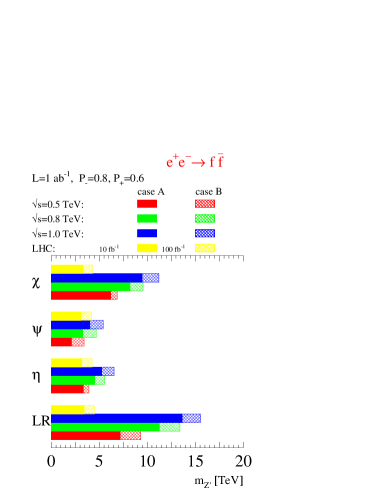
Below a Z′ resonance measurements of fermion-pair production are sensitive only to the ratio of Z′ couplings and Z′ mass. If a Z′ will be detected at the LHC its origin can be found by determining the Z′ couplings. Figure 3 demonstrates the resolution power between Z′ models assuming that the mass of the new boson is measured at the LHC. Here, leptonic final states are considered and lepton–universality is assumed.
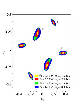
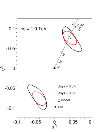
If the potential Z′ is heavier than 4.8 TeVand/or it does not couple to quarks, there will be no sensitivity to m at the LHC. Nevertheless, the analysis of fermion–pair production could detect a Z′ and resolve the model. Instead of extracting the Z′ couplings to fermions, , normalized Z′ couplings, , have to be obtained:
| (1) |
Assuming a Z′ with =5 TeV, its detection and identification will be possible as demonstrated in Figure 3. A Z′ is postulated with m=5 TeVand with leptonic couplings as suggested in the model. Measurements at =1 TeV with =1000 fb-1 and accuracies of =0.5%, =0.5% and =0.5% will allow to derive bounds on , as shown by the solid line. If =0.2% and =0.2% these bounds could be shrinked to the dashed-dotted line. On the line of the model the allowed area in the (plane is located around the point . Fixing the leptonic Z′ couplings to the model, a mass range of is derived for 0.5% and for 0.2, respectively.
It should be noted that a two-fold ambiguity in the signs of couplings remains since all observables are bilinear products of and .
2 limits
The limits on extra charged gauge bosons shown here are based on the two reactions (see Fig. 4a) and (see Fig. 4b) for three different models: the SM-type heavy (SSM ), the left-right model (LRM) and the SM-type Kaluza–Klein-excitation model (KK) [45]. The SM inputs , , , and are used in the numerics.
Details of the analysis based on can be found in Ref. [45]. In order to take into account detector acceptance, the photon energy, , and the angle of the photon with respect to the beam axis, , are restricted to the ranges and These cuts also remove singularities arising for soft or collinear photons. The photon’s transverse momentum is restricted to , where is the minimum angle down to which the veto detectors may observe electrons or positrons, here mrad. This cut removes the largest background, namely radiative Bhabha-scattering where the scattered and go undetected down the beam pipe.
Figure 6 shows the possible constraints (95% C.L.) on the right- and left-handed couplings of a to fermions using the total cross section and the left-right asymmetry as observables. The assumed systematic errors for are 0.5%(0.25%). 80% electron and 60% positron polarization are assumed. It is assumed in this figure that there exists a heavy SSM and that there is no signal from additional neutral gauge bosons. The couplings can only be constrained up to a two-fold ambiguity. This ambiguity could be resolved by reactions where the couples to a triple gauge vertex.
Details of the analysis based on can be found in Ref. [46]. In order to take into account detector acceptance, the angle of the detected quark relative to the beam axis is restricted to . The quark’s transverse momentum relative to the beam is restricted to for . This cut suppresses various SM backgrounds.
Figure 6 shows the possible constraints (95% C.L.) on SSM couplings to fermions for backscattered laser photons. The best limits come from the observable . The assumed systematic error of 2% dominates the statistical error, thus eliminating the potential gain from high luminosities. limits from backscattered laser photons are considerably better than those from Weizsäcker–Williams photons. Polarized beams give only a minor improvement to limits after including systematic errors. The couplings can only be constrained up to a two-fold ambiguity.
Table 1 shows mass sensitivity limits (95% C.L.) from both reactions for a predicted in the three models introduced above for different systematic errors. All assumptions are the same as in Figures 6 and 6. The limits on the SSM do not improve with polarized beams. The limits on the predicted in the LRM (KK) show a weak (considerable) improvement with polarized beams. As mentioned before, the limits do not improve much with polarized beams. Backscattered laser photons give important complementary limits relative to scattering.
| syst. error in % | 0.1 | 0.5 | 2.0 | 0.5 | 2.0 | 0.1 | 0.5 | 2.0 | 0.5 | 2.0 | |
|---|---|---|---|---|---|---|---|---|---|---|---|
| Model | |||||||||||
| SSM | 4.8 | 3.8 | 1.7 | 4.0 | 2.7 | 5.9 | 4.8 | 2.2 | 5.8 | 4.6 | |
| LRM | 1.3 | 1.1 | 0.9 | 0.7 | 0.6 | 1.7 | 1.4 | 1.2 | 1.2 | 1.1 | |
| KK | 5.0 | 4.0 | 1.8 | 5.7 | 3.8 | 6.4 | 5.1 | 2.3 | 8.2 | 6.5 | |
3 SO(10) neutrinos and E6 leptons
i) SO(10) neutrinos.
The fundamental representation of the SO(10) gauge group contains 16
fermions, which consist of the 15 fermions of one family in the
Standard Model (SM) and a
right-handed neutrino, which is a singlet under the SM gauge group.
Mixing between ordinary and heavy right-handed neutrinos induces new
couplings, which allow for the single production of the latter. Due to
the large contribution of the -channel
exchange, single Majorana neutrinos can be produced with masses close to
the total c.m. energy of the collider; for mixing parameters not
too tiny, , the production rates are large enough for
the states to be detected [47], see Fig. 7 a.
ii) E6 leptons. Twelve new fermions are needed to complete the 27 dimensional fundamental representation of E6. They consist of two weak isodoublet leptons, two isosinglet neutrinos, which can be either of the Dirac or Majorana type, and an isosinglet quark with charge appearing in a left- and a right-handed state:
Since the new fermions are either gauge singlets under the electroweak gauge group or vector-like there are no significant constraints on their masses and couplings from precision data. These particles can be pair produced via gauge boson exchange including a new boson related to an additional abelian factor in the gauge group structure at low energies. The cross sections for pair production of the heavy charged and neutral isodoublet leptons are rather large thus allowing for the discovery of these particles with masses close to the beam energy [48], as can be inferred from Fig. 7 b.
 |
 |
4 Heavy Majorana neutrinos in collisions
Throughout the TESLA physics studies, there has been the consideration that, in its electron-electron version, this machine can give unmistakable and irrefutable evidence for the existence of TeV-level Majorana neutrinos, should Nature have chosen to account in this way for the deficiencies of the Standard Model neutral-lepton sector. Recent evidence on possible neutrino oscillations has done little to clear up the broader picture of (i) the Majorana vs. Dirac character of the neutrinos and (ii) the disparity of masses of charged vs. neutral fermions in higher symmetry schemes.
The exchange of TeV-level Majorana neutrinos in high-energy scattering of left-handed electrons can lead to clear signals in the reaction . In addition, the energy dependence of those signals gives precise information on mass and couplings of the exchanged Majorana neutrino. Assuming a discovery limit of 8 events for an integrated luminosity of 500 fb-1 at GeVand 80% polarized electron beams, the discovery potential of TESLA ranges from about 1 TeV for smaller mixing to about 2 TeV for larger mixing , corresponding to the range of upper bounds allowed by experimental constraints [49]. These numbers scale approximately with the energy, i.e. for GeV the discovery limits are raised to 1.6 TeV and 3.2 TeV, respectively.
It has to be examined whether (a) such a process is excluded due to the non-observation of neutrinoless double beta decay, and (b) the greatest sensitivity to the possible existence of heavy right-handed singlets is offered by new and recently proposed experiments involving large tanks of double-beta-decay candidates such as germanium. Recently it has been demonstrated that the constraints on Majorana neutrinos imposed by these experiments turn out to be very weak if color effects and alternative contributions from e.g. supersymmetric particles or leptoquarks are properly taken into account [49]. TESLA is the one venue for cleanly interpretable experimentation, where the energy and helicities of the incoming electrons provide for clean identification and definition of the exchanged heavy neutral lepton.
5 Conclusions
Extensions of the SM gauge group lead to the existence of new heavy gauge bosons and and novel heavy fermions, the masses of which can be in the TeV range. and gauge bosons can be discovered with masses up to about 5 TeV at the LHC, while TESLA exceeds the sensitivity to masses up to TeV and SSM masses up to TeV via indirect virtual effects in leptonic processes. The couplings of these novel gauge bosons can be measured accurately at TESLA thanks to the high luminosities available at TESLA. The LHC will be the better environment for the search of new heavy quark states, while TESLA will discover novel heavy leptons with masses up to the kinematical limits. The comparison between TESLA and the LHC is summarized in Table 2.
| Alternative | TESLA | LHC |
|---|---|---|
| masses | TeV | TeV |
| couplings | (10%) | ? |
| SSM masses | TeV | TeV |
| couplings | (10%) | ? |
| SO(10), E6 fermions | leptons | quarks |
3 Top Quark Physics
The top quark is by far the heaviest fermion observed, yet all the experimental results tell us that it behaves exactly as would be expected for a third generation Standard Model (SM) quark with charge +2/3. In particular the direct measurement of the mass of the top quark by the CDF and D0 collaborations at the Tevatron, yielding a combined result of GeV, is in striking agreement with the earlier SM electroweak analysis of data recorded at LEP and SLC [50].
Its large mass, which is close to the scale of electroweak symmetry breaking, renders the top quark a unique object for studying the fundamental interactions in the attometer regime. It is likely to play a key role in pinning down the origin of electroweak symmetry breaking and in the search for clues to solve the flavour problem. If the Higgs mechanism should be verified then, for instance, the measurement of the top Yukawa coupling (see the section on Higgs bosons) would help to discriminate between SM and non-SM scenarios. High-precision measurements of the properties and interactions of top quarks are therefore mandatory at any future collider.
colliders are the most suitable instruments to study the properties of top quarks under clean experimental conditions. Operating the machine at the threshold, the mass of the top quark can be determined with an accuracy that is an order of magnitude superior to measurements at hadron colliders. A further asset is the availability of beam polarisation which is a powerful tool in precision studies of the neutral and charged current interactions of the top quark, both at threshold and in the continuum. These studies include accurate determination of the “static” properties of top quarks, its vector and axial vector couplings and its magnetic and electric dipole moment, as well as measurement of the charged-current couplings in the main decay channel. Moreover, decays of the top quark into novel particles, as predicted by extensions of the Standard Model, for instance into charged Higgs bosons and/or stop particles may be observed. The top-Higgs Yukawa coupling is best determined in the reaction discussed in section 2.
Since the lifetime of the quark is much shorter than the typical hadronisation time set by the scale , top quark production and decay can be analysed within perturbative QCD [51]. Unlike the case of light quarks the properties of the top quark, in particular its spin properties, are reflected directly in the distributions of the jets, bosons, or leptons into which the and decay. This additional important distinctive feature of top quarks will open up the rich phenomenology refered to above.
1 Profile of the top quark: decay modes
a) The Dominant SM Decay. The channel is the dominant top quark decay mode, not only in the Standard Model but also in extended scenarios. In the SM the total top width is, for all practical purposes, equal to the partial width of this decay mode. To lowest order
| (1) |
A large fraction, , of the decay bosons are longitudinally polarised. The proportionality of to the third power of is due to the fact that in the SM the longitudinal component, dominating for large masses, is to be identified with the charged Goldstone boson, the coupling of which grows with the mass. The width of the top quark is known to second-order QCD [52] and first-order electroweak corrections [53]. Numerically GeV for GeV (pole mass).
The direct measurement of the top quark width is difficult. The most promising method appears to be the extraction of the width from the forward-backward asymmetry of quarks near the production threshold. This asymmetry which is generated by the overlap of parity-even – and parity-odd –wave production channels is sensitive to the width . Including the other threshold observables, cross section and momentum distributions, a precision of about 10 % can be expected for the measurement of in total [54]. A more precise knowledge of , which should eventually be feasible, would allow an accurate determination of the CKM matrix elements via measurement of the respective branching ratios [55].
Chirality of the decay current. The precise determination of the weak isospin quantum numbers does not allow for large deviations of the decay current from the standard structure. Nevertheless, since admixtures may grow with the masses of the quarks involved ( through mixing with heavy mirror quarks of mass , for instance), it is necessary to check the chirality of the decay current directly. The energy distribution in the semileptonic decay chain depends on the chirality of the current. For couplings it is given by . Another SM prediction, which is important for helicity analyses, is that the charged lepton in the semileptonic (or the d-type quark in non-leptonic) decays of polarised top quarks is the best analyser of the top spin [56]: , where and are the top polarisation and the lepton direction of flight in the top rest frame, respectively.
A deviation from the standard current would change this distribution; in particular it would stiffen the energy spectrum and it would lead to a non-zero value of the energy distribution at the upper end-point. Extrapolating the analysis of [57] to the present TESLA design luminosity gives an experimental sensitivity to possible admixtures (corresponding to the form factor that measures ) which is listed in Table 1).
b) Non–Standard Top Decays. Such decays could occur, for example, in supersymmetric extensions of the Standard Model: top decays into charged Higgs bosons and/or into stop particles and neutralinos:
| (2) |
If kinematically allowed, branching ratios for these decay modes could be as large as for the Higgs and several percent for the SUSY decay Fig. 1 [58], given the present constraints on supersymmetric parameters. The signatures for these decay modes are very clear and they are easy to detect experimentally [59]. The subsequent decays of charged Higgs bosons manifest themselves through decays to and with rates which are different from the universal decay rates in the Standard Model, thus breaking vs. universality. If this decay exists it will first be seen at a hadron collider: perhaps at the Tevatron or eventually at the LHC. Nevertheless, at a Linear Collider additional important insight could be obtained into the coupling strength of the charged Higgs boson and its properties by measuring the branching ratio of this mode [59].
If neutralinos are the lightest supersymmetric particles, they escape undetected in stop decays, so that a large amount of missing energy would be observed in these decay modes. At a high luminosity linear collider this channel can be detected down to a branching fraction of slightly less than 1 percent [59].

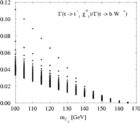
Besides breaking the law for the chirality of the decay current, mixing of the top quark with other heavy quarks would break the GIM mechanism if the new quark species do not belong to the standard doublet/singlet assignments of isospin multiplets. As a result, FCNC () couplings of order may be induced. FCNC quark decays, for example or , may therefore occur at the level of a few permille; down to this level they can be detected experimentally [60]. The large number of top quarks produced at the LHC allows, however, to search for rare FCNC decays with clean signatures, such as , down to a branching ratio of less than .
2 Threshold production: the top mass
Quark-antiquark production near the threshold in collisions is of great interest as it offers a unique way to investigate the bound-state dynamics of strongly interacting particles. The long lifetime of the lighter quarks allows the strong interactions to build up rich structures of bound states and resonances. For the top quark with its large mass and width, the picture is different: the decay time of the states is shorter than the revolution time of the constituents so that toponium resonances can no longer form [51]. Nevertheless, the remnants of the toponium -wave resonances induce a fast rise of the cross section near the threshold. The steep rise provides by far the best method for high-precision measurements of the top quark mass. In comparison to the reconstruction of the invariant mass of jets originating from a single top quark at future hadron colliders the LC threshold method is superior by an order of magnitude. This method has the advantage that the cross section for the production of a colour singlet state is analysed. Infering the mass of a coloured object like the top quark from the invariant mass of colour singlet final states recorded in the detector necessarily has a larger uncertainty.
Why should it be desirable to measure the top mass with high
precision? Two immediate reasons can be given:
The top mass is an important ingredient for the
electroweak precision analyses at the quantum level [61].
Suppose a Higgs boson has been found
at the Tevatron, the LHC
and/or the Linear Collider, and
its mass is known from
direct measurement.
If the and top quark masses are known to high precision then
the SM consistency checks, which at present provide an indirect
determination of
the mass of the Higgs particle,
will be substantially tightened.
In the case of TESLA
the Higgs mass can finally be
extracted from the high-precision electroweak observables to an
accuracy of about 5 % as shown in Fig. 8.
This would provide
the most stringent test of the Higgs mechanism
at the quantum level.
The Standard Model provides no understanding
of the disparate quark and lepton mass spectra,
and no answer to the question whether and how the fermion masses
and mixing angles are linked to each
other. This deficiency
might be removed by a future theory of flavor dynamics, still to be
discovered. The top quark, endowed with the heaviest
mass in the fermion sector, will very likely play a key role in this
context. In the same way as present measurements test the relations
between the masses of the electroweak vector bosons in the
Standard Model, similar relations between lepton and quark masses will
have to be scrutinized in the future.
The excitation curve can be predicted by perturbative QCD [62, 63, 64] because the rapid decay restricts the interaction region of the top quark to small distances. The interquark potential is given essentially by the short distance Coulombic part.
The excitation curve is built up primarily by the superposition of the states. At leading order in the non-relativistic expansion of the total cross section this sum can conveniently be performed by using Green function techniques and the Schrödinger equation:
| (3) |
The form and the height of the excitation curve are very sensitive to the mass of the top quark, Fig. 2a. Since any increase of the quark (pole) mass can be compensated by a rise of the QCD coupling, which lowers the energy levels, the measurement errors of the two parameters are positively correlated.
The correlation between the top mass and the QCD coupling can partially be resolved by measuring the momentum of the top quark [64] which is reflected in the momentum distribution of the decay boson. The momentum is determined by the Fourier transform of the wave functions of the overlapping resonances:
| (4) |
The top quarks will have average momenta of order . Together with the uncertainty due to the finite lifetime, this leads to average momenta of about 15 GeV for GeV, see Fig. 3.


Recently the next-to-next-to-leading order (NNLO) QCD corrections to the total cross section were calculated by several groups [68]. The corrections to the location of the threshold and the shift in the height of the cross section were found to be large. Top quark mass definitions, so-called threshold masses, were suggested [69] in this context that stabilise the location of the threshold with respect to the NNLO corrections. These threshold masses can be extracted from data with high accuracy and may then be converted into the frequently used mass parameter of the top quark [70]. (For a detailed comparison of the different approaches and an assessment of theoretical uncertainties, see [65].)

Fig. 4 shows the simulation of a scan of the cross section in the threshold region, including the effects of initial-state radiation and beamstrahlung, with 9 energy locations [67]. A two-parameter fit using the NNLO cross-section formulae yields the experimental sensitivity to the top mass and to the QCD coupling shown in Fig.5. This figure shows that only when the top mass is defined in the pole mass scheme there is a strong correlation with – but not for threshold masses. With the NNLO formulae that use threshold mass parameters, the following statistical errors can be achieved: , . These errors were derived for an integrated luminosity of . The theory errors in the determination of and were estimated by varying the renormalisation scale and by comparing NNLO with NLO results [67]. This analysis shows that the two-parameter fit is problematic in that absorbs almost all the uncertainties in the normalisation of , and these theoretical uncertainties are large. Hence determining from the cross section at threshold appears not to be the best procedure for the time being. However, a recent renormalisation-group improved calculation of the threshold cross section [71] leads to a considerable reduction of the theoretical uncertainty in the normalisation of the cross section down to 2-3%. The increase of the cross section from the exchange of a 115 GeV Standard Model Higgs boson [72] amounts to 5-8% and would give direct access to the top-Higgs Yukawa coupling.
Rather than using the top threshold scan to determine it is more effective to constrain its value to the current world average and fit the data to alone. With this strategy the statistical errors of the top mass determination decrease, being now 30 MeV for the and 40 MeV for the mass, while the theory errors, estimated as above, increase to 110 MeV for the and to 180 MeV for the mass. The larger theory error reflects the fact that due to the correlation between and the normalisation uncertainites are now shifted, into some extent, to the top mass.
A detailed assessment of the theoretical error must take into account the uncertainties due to i) different methods used in the NNLO calculations, ii) the dependence of a given NNLO cross-section formula, for a fixed convention with respect to the QCD coupling, on the definition of the top mass parameter and on the renormalisation scale, iii) uncalculated higher order corrections. Ref. [65] estimates that these uncertainties lead to an error on the mass of .
For the top mass measurements at the LHC a sensitivity of about 1 – 2 GeV was estimated [73], based on the reconstruction of top quarks from jet and lepton final states. Smearing effects due to soft stray gluons which are coherently radiated off the quark before the decay and off the quark after the decay, add to the complexity of the analysis. Thus, colliders will improve our knowledge on the top-quark mass by at least an order of magnitude.
Polarised Beams and the Top Threshold [74]: Close to threshold beam polarisation will be particularly useful to determine the weak couplings responsible for top production and decay. The left right asymmetry [75] can be measured to an accuracy of 0.01, if an integrated luminosity of 100 fb-1 is distributed evenly among the four combinations of beam polarisations ( and will be assumed throughout). If 300 fb-1 are invested specifically into the L-R and R-L combinations of electron-positron helicities, even can be achieved. Such a measurement would determine the vector coupling of top quarks to a relative precision of 2% (or even 0.8%) and thus become sensitive to the quantum corrections [76].
Both top quarks and antiquarks will be highly polarised, with and 0.88 respectively for the L-R and R-L helicity combinations. For the decay channel this allows to constrain the coefficient of the lepton angular distribution [56] to better than 0.02 and 0.008, respectively, for the two assumptions on the luminosity. By the same line of reasoning the (energy dependent) angular distribution of neutrinos can be analysed and the combination of these measurements will lead to tight limits on anomalous couplings of the top quark [77].
Polarised beams would also play an important role in the study of the angular distribution and the transverse and the normal polarisation of the top quarks. These are sensitive to the axial coupling of the top quark and to the potential through rescattering corrections [76].
Last but not not least, top quark polarisation will be extremely useful for the analysis of non-standard decays. The parameter in the angular distribution of a charged Higgs boson [78] from the decay can be measured to 0.04 (or even 0.016) which will lead to important constraints on the handedness of the Yukawa coupling.
3 Continuum production and form factors
The main production mechanism for top quarks in collisions is the annihilation channel
Extensive theoretical knowledge has been gained about the total cross section for this reaction: The QCD corrections were determined to order [79] and the electroweak SM corrections to 1-loop order [80], including the hard photon corrections [81]. The 1-loop quantum corrections to the lowest-order cross section were also computed for the minimal supersymmetric extension of the SM [82]. As shown in Fig. 6, the cross section is of the order of 1 pb so that top quarks will be produced at large rates in a clean environment at linear colliders; about 300,000 pairs for an integrated luminosity of .

The production and decays of top quarks are not significantly affected by the non-perturbative effects of hadronisation. Moreover, the perturbative QCD corrections are small for the continuum production of pairs in a general spin configuration [85], for the decay of polarized top quarks [56], and for the QCD rescattering corrections sufficiently away from threshold [86]. Therefore the helicities of the top quarks can be determined from the distribution of the jets and leptons in the decay chain and the neutral and charged-current interactions of the top quark can be measured with good accuracy.
An obvious question is whether the top quark has non-standard
couplings to gauge bosons. Possible anomalous couplings of the top
quark to bosons can be parameterized by means of
an effective Lagrangian or, alternatively, by using form factors.
The form factors of the top quark
in the electromagnetic
and the weak neutral currents are the Pauli–Dirac form factors
and , the axial form
factors ,
and the CP-violating form factors
(see e.g. [87, 88]).
Suffice it to mention that the physical object is the
S-matrix element: in some models, for instance in supersymmetric SM
extensions,
the new physics contributions to the
amplitude are not confined to the
vertices [82, 89].
By convention, to lowest order in the SM
the chirality-conserving
form factors
and are
normalized to unity, whereas and , which
are chirality-flipping,
vanish to this order. Anomalous values could be a consequence of
strong-interaction-type electroweak symmetry breaking scenarios or of
composite quark structures. Detectable values of the
electric-type dipole moments would be
evidence for a new CP-violating interaction beyond the
Kobayashi-Maskawa mechanism.
Because the above form factors are functions of the time-like
energy variable they can have, apart from dispersive also
non-zero absorptive parts if (new) physics thresholds are crossed.
For the production vertex
this amounts to
real and imaginary parts, respectively.
Depending on how the
form factors vary with their contribution to the
cross section or to other observables can increase with the c.m. energy.
The general amplitude for the decay contains
four (complex) form factors, two chirality-conserving
and two chirality-flipping ones, respectively. Here we consider only
the form factor which signifies a
+ admixture, and
which, if found to be non-zero, would be
evidence for non-SM CP violation [88].
(For further studies, see [90].)
Among the “static” parameters, that is, the above
form factors of the top quark which can be
determined only at linear colliders, the following
examples are of particular interest:
charges of the top quark. The form factors
can be determined from the production cross sections
with and beams and the left-right asymmetry
[91, 92]. Moreover, the production of top quarks near the
threshold with longitudinally polarised beams leads to a sample of
highly polarised quarks. The small admixture of transverse and normal
polarisation induced by –wave/–wave interference, is extremely
sensitive to the axial charge of the top quark [76].
Some models of strong-interaction-type electroweak symmetry breaking
predict rather large anomalous contributions,
up to 10 [93].
Magnetic dipole moments of the top quark. These form
factors are generated already in the SM at the quantum level.
Gluon exchange induces a term
and the interactions of a light Higgs boson would lead to
a contribution of similar size. If the
electrons in the annihilation process are left-handedly polarised, the top quarks are
produced preferentially as left-handed particles in the forward
direction while only a small fraction is produced as right-handed
particles in the backward direction [94]. As a result of this
prediction in the Standard Model, the backward direction is most
sensitive to small anomalous magnetic moments of the top quarks. The
anomalous magnetic moments can thus be searched for by
measuring the angular dependence of the quark cross section
[94, 57].
| Form factor | SM value | = 500 GeV | = 800 GeV | ||
|---|---|---|---|---|---|
| = 0 | = – 0.8 | = 0 | = – 0.8 | ||
| 1 | 0.019 | ||||
| 1 | 0.016 | ||||
| 0 | 0.015 | 0.011 | 0.011 | 0.008 | |
| 0 | 0.035 | 0.007 | 0.015 | 0.004 | |
| [10-19 e cm] | 0 | 20 | 4 | 8 | 2 |
| 0 | 0.012 | 0.008 | 0.008 | 0.007 | |
| [10-19 e cm] | 0 | 7 | 5 | 5 | 4 |
| 0 | 0.010 | 0.008 | 0.006 | 0.005 | |
| 0 | 0.055 | 0.010 | 0.037 | 0.007 | |
| 0 | 0.030 | 0.012 | |||
| 0 | 0.025 | 0.010 | |||
Electric dipole moments of the top quark. Electric dipole moments of detectable size can be generated only by new CP-violating interactions. If a light neutral Higgs boson ( 160 GeV) with undefined CP parity exits, its reduced scalar and pseudoscalar couplings to top quarks could be of order 1 which leads to CP-violating form factors that can be sizeable not too far away from the threshold [97]: at = 370 GeV , Re Im 2 - 3 , and . At a high luminosity LC these effects could be measured with (optimized) CP-odd observables [88, 95, 98]. The exchange of supersymmetric particles involving new CP-violating phases [95, 99, 89] leads to smaller effects.
The results of a number of sensitivity analyses are given in Table 1. Most of these studies were performed at the parton level. Only the dilepton and single lepton decay channels () were considered. A possible strategy for performing these multi-parameter analyses in future experiments is as follows. First one may measure CP-odd angular correlations and asymmetries which are sensitive only to CP-violating form factors. Observables were constructed which can be used to disentangle possible CP effects in production and decay [88, 95]. Once the values of – or limits to – these form factors are known, one can proceed by measuring the CP-invariant moments in production and decay by suitable distributions and asymmetries (see above). In this way one probes for anomalous effects down to length scales of a few cm. It is worth emphasizing one aspect of such studies. At linear colliders very clean and sensitive searches can be made for new CP-violating sources which may only become visible at high energies, in particular in production and decay. Detection of such interactions in the laboratory would have striking consequences for our attempts to understand the matter-antimatter asymmetry of the universe.
4 Complementarity with the LHC
Finally a brief comparison of some of the respective assets of the proposed TESLA collider (LC) and the LHC is in order. As far as as top quark physics is concerned these machines are complementary, to a large extent, in their potential. (For a recent compilation of the perspectives of top quark physics at the LHC, see [73].) Clearly, a remarkable feature of the LC is the possiblity to extract the mass of the top quark from the threshold excitation curve with an error estimated below 200 MeV. Also the total top decay width can be determined with a relative error of about 10. At the LHC top mass measurements are expected to be feasible with an accuracy of about 1 - 2 GeV. As far as is concerned no sensible method of extraction is known. However, from single top quark production at the LHC the measurement of the Kobayashi-Maskawa matrix element to 10 appears feasible.
At the LC very clean and accurate measurements of the neutral current couplings of the top quark to the photon and Z-boson – its vector and axial vector charges, anomalous magnetic and electric dipole moments – can be made, both at threshold and in the continuum. A powerful tool for these studies and those of the charged current couplings will be the possiblity of polarising the beams.
Owing to the expected production of or more top quark pairs per year the LHC has a large discovery potential of a number of non-standard rare top decays, such as the flavour-changing neutral current reactions , down to branching ratios of about which is superior to the LC. If top decays into charged Higgs bosons exist they should be seen first at hadron colliders. Then at the LC rather precise measurements of the branching fraction and clean polarisation studies can be made, offering insights into the Yukawa interactions at work in this mode. Moreover, the LC allows for very sensitive searches of the supersymmetric decay of the top quark into stop and neutralino particles.
4 Quantum Chromodynamics
1 Introduction
Strong-interaction measurements at TESLA will form an important component of the physics programme. The collider offers the possibility of testing QCD [102] at high energy scales in the experimentally clean, theoretically tractable environment. In addition, virtual interactions will be delivered free by Nature, and a dedicated collider is an additional option, allowing detailed measurements of the relatively poorly understood photon structure. The benchmark physics main topics are:
Precise determination of the strong coupling .
Measurement of the evolution of and constraints on the GUT scale.
Measurement of the total cross section and the photon structure function.
2 Precise determination of
The current precision of individual measurements is limited at best to several per cent [103]. Since the uncertainty on translates directly into an uncertainty on perturbative QCD (pQCD) predictions, especially for high-order multijet processes, it would be desirable to achieve much better precision. In addition, since the weak and electromagnetic couplings are known with much greater relative precision, the error on represents the dominant uncertainty on our ‘prediction’ of the scale for grand unification of the strong, weak and electromagnetic forces [104].
Here we will refer to the conventional yardstick of quoted at the mass scale, , unless explicitly stated otherwise. Several techniques for determination will be available at TESLA:
Event shape observables
The determination of from event ‘shape’ observables that are sensitive to the 3-jet nature of the particle flow has been pursued for two decades and is generally well understood [105]. In this method one usually forms a differential distribution, makes corrections for detector and hadronisation effects, and fits a pQCD prediction to the data, allowing to vary. Examples of such observables are the thrust, jet masses and jet rates.
The latest generation of such measurements, from SLC and LEP, has shown that statistical errors below 0.001 can be obtained with samples of a few tens of thousands of hadronic events. With the current TESLA design luminosities of /cm2/s, at = 500 (800) GeV, hundreds of thousands of e+e- events would be produced each year, and a statistical error on below 0.0005 could be achieved.
Detector systematic errors, which relate mainly to uncertainties on the corrections made for acceptance and resolution effects and are observable-dependent, are under control in today’s detectors at the = 0.001–0.004 level [106]. If the TESLA detector is designed to be very hermetic, with good tracking resolution and efficiency, as well as good calorimetric jet energy resolution, all of which are required for the search for new physics processes, it seems reasonable to expect that the detector-related uncertainties can be beaten down to the 0.001 level or better.
, or events will present significant backgrounds to events for QCD studies, and the selection of a highly pure event sample will not be quite as straightforward as at the resonance. The application of kinematic cuts would cause a significant bias to the event-shape distributions, necessitating compensating corrections at the level of 25% [107]. More recent studies have shown [108] that the majority of events can be excluded without bias by using only events produced with right-handed electron beams for the analysis. Furthermore, the application of highly-efficient -jet tagging can be used to reduce the contamination to the 1% level. After statistical subtraction of the remaining backgrounds (the and event properties have been measured accurately at SLC and LEPI/II), the residual bias on the event-shape distributions is expected to be under control at the better than 0.001 level on .
Additional corrections must be made for the effects of the smearing of the particle momentum flow caused by hadronisation. These are traditionally evaluated using Monte Carlo models. The models have been well tuned at SLC and LEP and are widely used for evaluating systematic effects. The size of the correction factor, and hence the uncertainty, is observable dependent, but the ‘best’ observables measured at the have uncertainties as low as 0.001. Furthermore, one expects the size of these hadronisation effects to diminish with c.m. energy at least as fast as 1/. Hence 10%-level corrections at the should dwindle to 1%-level corrections at 500 GeV, and the associated uncertainties will be substantially below the 0.001 level on . This has been confirmed by explicit simulations using PYTHIA [106].
Currently pQCD calculations of event shapes are available complete only up to , although resummed calculations are available for some observables [109]. One must therefore estimate the possible bias inherent in measuring using the truncated QCD series. Though not universally accepted, it is customary to estimate this from the dependence of the fitted value on the QCD renormalisation scale, yielding a large and dominant uncertainty of about 0.006 [105]. Since the missing terms are , and since (500 GeV) is expected to be about 25% smaller than , one expects the uncalculated contributions to be almost a factor of two smaller at the higher energy. However, translating to the yardstick yields an uncertainty of 0.005, only slightly smaller than currently. Therefore, although a 0.001-level measurement is possible experimentally, it will not be realised unless contributions are calculated. There is reasonable expectation that this will be achieved within the next 5 years [110].
The System
The dependence of the production cross section, , on the top-quark mass, , and on is discussed in section 2. In order to optimise the precision on the measurement near threshold it is desirable to input a precise measurement from elsewhere. Furthermore, the current theoretical uncertainty on translates into = . Hence, although extraction of from near threshold may provide a useful ‘sanity check’ of QCD in the system, it does not appear currently to offer the prospect of a competitive measurement. A preliminary study has also been made [111] of the determination of from above threshold. For 500 GeVthe uncertainty on due to is around 0.0005. The limiting precision on will be given by the uncertainty on the luminosity measurement. If this is as good as 0.5% then could be determined with an experimental precision approaching 0.001, which would be extremely valuable as a complementary precision measurement from the system.
A high-luminosity run at the Z resonance
A Giga sample offers two additional options for determination via measurements of the inclusive ratios and . Both are indirectly proportional to , and hence require a very large event sample for a precise measurement. For example, the current LEP data sample of 16 M yields an error of 0.0025 on from . The statistical error could, naively, be pushed to below the = 0.004 level, but systematic errors arising from the hadronic and leptonic event selection will probably limit the precision to 0.0008 (see section 1). This would be a very precise, reliable measurement. In the case of the experimental precision from LEP and CLEO is already at the 0.001 level on . However, there has been considerable debate about the size of the theoretical uncertainties, with estimates as large as 0.005 [112]. If this situation is clarified, and the theoretical uncertainty is small, may offer a further 0.001-level measurement.
3 evolution of
In the preceeding sections we discussed the expected attainable precision on the yardstick . Translation of the measurements of () () to requires the assumption that the ‘running’ of the coupling is determined by the QCD function. However, since the logarithmic decrease of with is an essential component of QCD, reflecting the underlying non-Abelian dynamics, it is vital also to test this -dependence explicitly. Such a test would be particularly interesting if new coloured particles were discovered, since deviations from QCD running would be expected at energies above the threshold for pair-production of the new particles. Furthermore, extrapolation of to very high energies of the order of GeVcan be combined with corresponding extrapolations of the dimensionless weak and electromagnetic couplings in order to constrain the coupling-unification, or GUT, scale [104]. Hence it would be desirable to measure in the same detector, with the same technique, and by applying the same treatment to the data at a series of different energies , so as to maximise the lever-arm for constraining the running.
Simulated measurements of () at = 91, 500 and 800 GeVare shown in Fig. 1, together with existing measurements which span the range GeV. The highest-energy measurements are currently provided by LEPII. The point at = 91 GeVis based on the technique, and those at 500 and 800 GeVare based on the event shapes technique. The last two include the current theoretical uncertainty, which yields a total error on each point equivalent to = 0.004. It is clear that the TESLA data would add significantly to the lever-arm in , and would allow a substantially improved extrapolation to the GUT scale.
4 Further important topics
Limited space allows only a brief mention of several other important topics [113]:
Hard gluon radiation in events would allow several tests of the strong dynamics of the top quark [114]: test of the flavour-independence of strong interactions; limits on anomalous chromo-electric and/or chromo-magnetic dipole moments [115]; determination of the running .
Soft gluon radiation in events is expected to be strongly regulated by the large mass and width of the top quark. Precise measurements of gluon radiation patterns in events would provide additional constraints on the top decay width [116].
Polarised electron (and positron) beams can be exploited to test symmetries using multi-jet final states. For polarized annihilation to three hadronic jets one can define , which correlates the electron-beam polarization vector with the normal to the three-jet plane defined by and , the momenta of the two quark jets. If the jets are ordered by momentum (flavour) the triple-product is CP even (odd) and T odd. Standard Model T-odd contributions of this form are expected [117] to be immeasurably small, and limits have been set for the system [118]. At TESLA these observables will provide an additional search-ground for anomalous effects in the system.
The difference between the particle multiplicity in heavy- () and light-quark events is predicted [119] to be independent of c.m. energy. Precise measurements have been made at the , but measurements at other energies are statistically limited in precision, rendering a limited test of this important prediction. High-precision measurements at TESLA would add the lever-arm for a powerful test.
Colour reconnection and Bose-Einstein correlations are important to study precisely since they may affect the precision with which the masses of heavy particles, such as the and top-quark, can be reconstructed kinematically via their multijet decays [120].
Hadronisation studies and renormalon physics can be explored via measurements of event-shape observables over a range of values.
5 Two Photon physics
Traditionally colliders provide a wealth of two-photon data. The photons are produced via bremsstrahlung [121] from the electron and positron beam, which leads to a soft energy spectrum of the photons. Such processes will also occur at future high energy colliders. Due to the single use of the colliding beams at these machines other operation modes become possible such as a collider and e collider [122, 123], where the electron beam(s) of a linear collider are converted into photon beams via Compton laser backscattering. This offers the exciting possibility to study two-photon interactions at the highest possible energies with high luminosity. A plethora of QCD physics topics in two-photon interactions can be addressed with a linear collider or collider. Furthermore, good knowledge and understanding of two photon processes will be essential for controlling background contributions to other processes.
Total cross section
At a linear collider and collider detailed properties of two-photon collisions can be studied. A key example is the total cross-section, which is not yet understood from first principles. Fig. 2 shows present photon-photon cross-section data in comparison with recent phenomenological models [124]. All models predict a rise of the cross-section with the collision energy . The predictions for high energies show dramatic differences reflecting our present lack in understanding. In proton-like models (solid curve [125] ), the rise follows closely that of the proton-proton cross-section, while in QCD based models (upper [126] and lower [124] bands), the rise is obtained using the eikonalized pQCD jet cross-section.
A detailed comparison of the predictions reveals that in order to distinguish between all the models the cross-sections need to be determined to a precision of better than 10% [124] at a future 0.5–1 TeV collider. This is difficult to achieve at an collider, since the variable needs to be reconstructed from the visible hadronic final state in the detector. At the highest energies the hadronic final state extends in pseudorapidity in the region , while the detector covers roughly the region . Some information can be gained by measuring the total integrated cross section above a value , e.g. GeV, for which the total spread of the model predictions is 10-20% [127].
For a collider the photon beam energy can be tuned with a spread of less than 10%, such that measurements of can be made at a number of “fixed” energy values in e.g. the range GeV, as shown in Fig. 2. The absolute precision with which these cross-sections can be measured ranges from 5% to 10%, where the largest contributions to the errors are due to the control of the diffractive component of the cross-section, Monte Carlo models used to correct for the event selection cuts, the knowledge on absolute luminosity and shape of the luminosity spectrum [127]. It will be necessary to constrain the diffractive component in high energy two-photon data. A technique to measure diffractive contributions separately, mirrored to the rapidity gap methods used at HERA, has been proposed in [128].
While the absolute cross-sections are measured with limited precision, the change of the cross-section with energy can be determined much more accurately. Fitting the data of the collider to the Regge inspired form in the high energy region, one can determine with a precision of . The models show a variation between and .
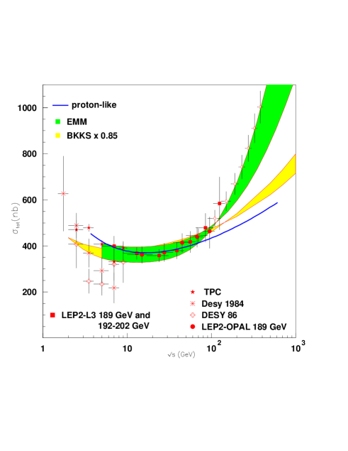
Photon structure
The nature of the photon is complex. A high energy photon can fluctuate into a fermion pair or even into a bound state, i.e. a vector meson with the same quantum numbers as the photon . These quantum fluctuations lead to the so-called hadronic structure of the photon. In contrast to the proton, the structure function of the photon is predicted to rise linearly with the logarithm of the momentum transfer , and to increase with increasing Bjorken- [129]. The absolute magnitude of the photon structure function is asymptotically determined by the strong coupling constant [130].
The classical way to study the structure of the photon is via deep inelastic electron-photon scattering (DIS), i.e. two-photon interactions with one quasi-real (virtuality ) and one virtual ( few GeV2) photon. The unpolarised e DIS cross-section is
| (1) |
where denote the structure functions of the real photon. To leading order the structure function is given by the quark content, e.g.
| (2) |
To measure it is important to detect (tag) the scattered electron which has emitted the virtual photon. Background studies suggest that these electrons can be detected down to 25 mrad and down to 50 GeV. For e scattering at an e collider the energy of the probed quasi-real photon is known (within the beam spread of 10%) and the systematic error can be controlled to about 5%. Fig. 3 shows the measurement potential for an e collider [131]. The measurements are shown with statistical and (5%) systematical error, for 20 fb-1 e collider luminosity, i.e. about a year of data taking. Measurements can be made in the region , in a region similar to the HERA proton structure function measurements, and GeV2. The cross-sections at low- constitutes 30-40% of charm, and corrections due to amount to more than 10% for the region , and can thus be studied. For the collider mode the hadronic final state needs to be measured accurately in order to reconstruct . This will limit the lowest reachable value to be around , but allows for measurements in the high () and high ( GeV2) range, for detailed QCD evolution tests [132].

At very high values ( GeV2) also and exchange will become important, the latter leading to charged current events [133] yielding events with large missing transverse momentum due to the escaping neutrino. By measuring the electroweak neutral and charged current structure functions, the up and down type quark content of the photon can be determined separately.
While e scattering allows to measure the quark distributions it only weakly constrains the gluon distribution via the QCD evolution of the structure functions. Direct information on the gluon in the photon can however be obtained from measurements of jet [134], open charm [135], and [136] production in interactions at an and collider. Values of down to a few times 10-3 can be reached with charm and di-jet measurements [134, 135], a region where predicted gluon distributions typically differ by a factor of two or more.
A linear collider also provides circularly polarised photon beams. This offers a unique opportunity to study the polarised parton distributions of the photon, for which to date no experimental data are available.
Information on the spin structure of the photon can be obtained from inclusive polarised deep inelastic e measurements and from jet and charm measurements [137, 138] in polarised scattering. An example of a jet measurement is presented in Fig. 4 which shows the asymmetry measured for dijet events, for the and collider modes separately. Two extreme models are assumed for the polarised parton distributions in the photon. Already with very modest luminosity significant measurements of the polarised parton distributions can be made at a linear collider. The extraction of the polarised structure function , with the polarised parton densities, can however be best done at an e collider. Measurements of , particularly at low , are very important for studies of the high energy QCD limit, or BFKL regime [139]. Indeed, the most singular terms of the effects of small resummation on behave like , compared to in the unpolarised case of . Thus large effects are expected to set in much more rapidly for polarised than for unpolarised structure measurements. Leading order calculations, which include kinematic constraints, show that differences in predictions of with and without these large logarithms can be as large as a factor 3 to 4 for and can be measured with a few years of data taking at a collider.

Testing of BFKL dynamics
Dedicated measurements have been proposed for detecting and studying the large logarithm resummation effects in QCD. Experimentally establishing the BFKL effect in data is very important for the understanding of the high energy limit in QCD scattering.
The most promising measurement for observing BFKL effects is the total cross-section, i.e. the scattering of two virtual photons with approximately equal virtualities [140]. This cross section can be calculated entirely within pQCD and is found to be sufficiently large. The events are measured by tagging both scattered electrons. At a 500 GeV collider about 3000 events are expected per year (200 fb-1) and a factor of 3 less in the absence of BFKL effects [141]. The ability to tag electrons down to as low angles as possible (e.g. 25 mrad) is essential for this measurement. The growth of the cross section as function of due to the BFKL effect is shown in Fig. 5, (solid line) and compared with the cross section in absence of BFKL (dashed line).
Closely related to the measurement is vector meson production, e.g or (at large ) , where the hard scale in the process is given by the mass or the momentum transfer . ’s can be detected via their decay into leptons, and separated from the background through a peak in the invariant mass. Approximately 100 fully reconstructed 4-muon events are expected for 200 fb-1 of luminosity for a 500 GeV collider [142]. For this channel it is crucial that the decay muons and/or electrons can be measured to angles below 10 degrees in the experiment.
6 Complementarity of LHC
QCD studies at the LHC will concentrate mainly on: jet studies, extracting parton densities in the proton, hard diffraction and heavy quark studies [145]. In principle QCD phenomena can be studied at scales upto a few TeV. A precision measurement of is foreseen via jet cross section measurements, but the precision has not been quantified yet. BFKL phenomena can be studied mainly via di-jet production using jet pairs with a large rapidity difference, which has an entirely different systematics compared to the methods proposed for the linear collider.
Recently [146] it was proposed to study real two photon processes at the LHC. If the technical challenges to tag the outgoing protons can be overcome, such data could allow for exploratory studies of quasi real two-photon physics in the high energy regime, such as the total cross section and jet production studies.
References
-
[1]
A. Pukhov et al.
CompHEP: A Package for Evaluation of Feynman Diagrams
and Integration over Multiparticle Phase Space. User’s Manual for
Version 33.
hep-ph/9908288;
E. Boos, M. Dubinin. Single W-boson Production at Linear Colliders. hep-ph/9909214. -
[2]
S. Jadach et al.
Phys. Lett., B417:326, 1998;
S. Jadach et al. Phys. Rev., D61:113010, 2000. -
[3]
K.J.F. Gaemers, G.J. Gounaris.
Z. Phys., C1:259, 1979;
K. Hagiwara et al. Nucl. Phys., B282:253, 1987. - [4] W. Menges. A Study of Charged Current Triple Gauge Couplings at TESLA. LC-PHSM-2001-022.
- [5] M. Kuroda et al. Phys. Lett., B183:366, 1987.
- [6] A. Blondel. Phys. Lett., B202:145, 1988.
- [7] K. Mönig. The Use of Positron Polarization for Precision Measurements. LC-PHSM-2000-059.
-
[8]
A. Denner et al.
Phys. Lett., B475:127, 2000;
A. Denner et al. EPJdirect Vol. 2, C4:1, 2000;
A. Denner et al. Nucl. Phys., B587:67, 2000. -
[9]
P. Ciafaloni, D. Comelli.
Phys. Lett., B446:278, 1999;
M. Ciafaloni et al. Phys. Rev. Lett., 84:4810, 2000;
M. Ciafaloni, P. Ciafaloni, D. Comelli. Nucl. Phys., B589:359, 2000;
W. Beenakker, A. Werthenbach. Phys. Lett., B489:148, 2000;
M. Hori, H. Kawamura, J. Kodaira. Phys. Lett., B491:275, 2000;
J.H. Kühn, A.A. Penin, V.A. Smirnov. Eur. Phys. J., C17:97, 2000;
V.S. Fadin et al. Phys. Rev., D61:094002, 2000;
M. Melles. Resummation of Yukawa Enhanced and Subleading Sudakov Logarithms in Longitudinal Gauge Boson and Higgs Production, hep-ph/0012157. - [10] S. Alam. Phys. Rev., D50:124, 1994.
- [11] A. Arhrib, J.-L. Kneur, G. Moultaka. Radiative Contributions to TGC in the MSSM. hep-ph/9603268; in: DESY 96-123D (see Ref. [100]).
- [12] S.Y. Choi, F. Schrempp. Phys. Lett., B272:149, 1991.
- [13] V. Barger, T. Han, R.J.N. Phillips. Phys. Rev., D39:146, 1989.
- [14] G. Belanger, F. Boudjema. Phys. Lett., B288:201, 1992.
- [15] W.J. Stirling, A. Werthenbach. Eur. Phys. J., C14:103, 2000.
- [16] M. Grünewald et al. Four Fermion Production in Electron Positron Collisions. hep-ph/0005309; in: Report of the Four-fermion working group of the LEP2 Monte Carlo Workshops, CERN, 1999/2000.
- [17] R. Hawkings, K. Mönig. EPJdirect Vol. 1, C8:1, 1999.
- [18] K. Mönig. Measurement of the Differential Luminosity using Bhabha Events in the Forward-Tracking Region at TESLA. LC-PHSM-2000-060.
- [19] A. Gurtu. Precision Tests of the Electroweak Gauge Theory. Talk presented at the ICHEP2000 conference, July 27 - August 2, 2000, Osaka, Japan.
- [20] M. Winter. Determination of the Strong Coupling Constant at Giga-Z. LC-PHSM-2001-016.
- [21] M. Consoli, W. Hollik, F. Jegerlehner. Electroweak Radiative Corrections for Physics. CERN 89-08, (Vol. 1):7, 1989.
- [22] G. Wilson. Precision Measurement of the W Mass with a Polarised Threshold Scan at a Linear Collider. LC-PHSM-2001-009.
- [23] S. Eidelmann, F. Jegerlehner. Z. Phys., C67:585, 1995.
- [24] F. Jegerlehner. The Effective Fine Structure Constant at TESLA Energies. LC-TH-2001-035.
- [25] Z. Zhao. Measurement of at 2-5 GeV. Talk presented at the ICHEP2000 Conference, July 27 - August 2, 2000, Osaka, Japan.
-
[26]
S. Heinemeyer, Th. Mannel, G. Weiglein.
Implications of Results from - and -Threshold Running.
hep-ph/9909538;
J. Erler et al. Phys. Lett., B486:125, 2000. - [27] G. Altarelli, R. Barbieri, F. Caravaglios. Phys. Lett., B349:145, 1995.
- [28] M.E. Peskin, T. Takeuchi. Phys. Rev., D46:381, 1992.
-
[29]
J. Gunion.
Talk presented at LCWS2000, FNAL, October 24-28, 2000;
P. Chankowski et al. Phys. Lett., B496:195, 2000. - [30] J. Letts, P. Mättig. Direct Determination of the CKM Matrix from Decays of W Bosons and Top Quarks at High Energy Colliders. LC-PHSM-2001-008.
- [31] Particle Data Group, D.E. Groom et al. Eur. Phys. J., C15:1, 2000.
- [32] BaBar Collaboration. Report of the BaBar Physics Workshop. SLAC-R-504, 1998.
- [33] M. Paulini. Int. J. Mod. Phys., A14:2791, 1999.
- [34] ATLAS Collaboration. Detector and Physics Performance Technical Design Report, Vol. 2. CERN/LHCC 99-15.
- [35] LHCb Collaboration. Technical Proposal. CERN/LHCC 98-4.
- [36] A. Ali et al. Quark Physics with Bosons. LC-TH-2001-018.
- [37] G. Buchalla, G. Hiller, G. Isidori. Phys. Rev., D63:014015, 2001.
- [38] G. Hiller, A. Kagan. Probing for New Physics in Polarized Decays at the . SLAC-PUB-8752.
- [39] J.I. Illana, T. Riemann. Charged Lepton Flavour Violation from Massive Neutrinos in Z Decays. hep-ph/0010193, accepted by Phys. Rev., D.
-
[40]
M.J. Levine.
Phys. Rev., D36:1329, 1987;
F. Gabbiani, J.H. Kim, A. Masiero. Phys. Lett., B214:398, 1988. - [41] M. Frank, H. Hamidian. Phys. Rev., D54:6790, 1996.
-
[42]
A. Djouadi, A. Leike, T. Riemann, D. Schaile, C. Verzegnassi.
Z. Phys., C56:289, 1992;
A. Leike, S. Riemann. Z. Phys. C75:341, 1997;
S. Riemann. Study of ’ Couplings to Leptons and Quarks at NLC. hep-ph/9610513. In: Proceedings of the 1996 DPF / DPB Summer Study on New Directions for High-energy Physics;
R. Casalbuoni, S. De Curtis, D. Dominici, R. Gatto, S. Riemann. ’ Indication from new APV Data in Cesium and Searches at Linear Colliders. LC-TH-2000-006, hep-ph/0001215. -
[43]
S. Godfrey.
Phys. Rev., D51:1402, 1995;
ATLAS Collaboration. Technical Design Report. CERN-LHCC 99-15. - [44] S. Riemann. Predictions for and Related Reactions. LC-TH-2001-007 and Proceedings LCWS2000, Fermilab 2000.
- [45] S. Godfrey, P. Kalyniak, B. Kamal, A. Leike. Phys. Rev., D61:113009, 2000, hep-ph/0001074.
- [46] M. Doncheski, S. Godfrey, P. Kalyniak, B. Kamal, A. Leike. Discovery and Identification of ’ Bosons in . hep-ph/0008157, to appear in Phys. Rev., D.
- [47] W. Buchmüller, C. Greub. Nucl. Phys., B363:345, 1991.
- [48] J.L. Hewett, T.G. Rizzo. Phys. Rep., 183:193, 1989, and references therein.
- [49] C.A. Heusch, P. Minkowski. Int. J. Mod. Phys., A15:2429, 2000.
- [50] Particle Data Group, D.E. Groom et al. Eur. Phys. J., C15:1, 2000. Particle Data Group web page
-
[51]
J.H. Kühn.
Act. Phys. Pol., B12:347, 1981;
I.I. Bigi, Y.L. Dokshitzer, V.A. Khoze, J.H. Kühn, P.M. Zerwas. Phys. Lett., B181:157, 1986. -
[52]
M. Jeżabek, J.H. Kühn.
Nucl. Phys., B314:1, 1989;
A. Czarnecki, K. Melnikov. Nucl. Phys., B544:520, 1999;
K.G. Chetyrkin et al. Phys. Rev., D60:114015, 1999. -
[53]
A. Denner, T. Sack.
Nucl. Phys., B358:46, 1991;
G. Eilam et al. Phys. Rev. Lett., 66:3105, 1991. -
[54]
H. Murayama, Y. Sumino.
Phys. Rev., D47:82, 1993;
K. Fujii, T. Matsui, Y. Sumino. Phys. Rev., D50:4341, 1994;
P. Comas et al. The Physics of the Threshold Scan. In: DESY 96-123D (see Ref.[100]);
D. Schulte et al. In: Conceptual Design of a 500 GeV Linear Collider with Integrated X-ray Laser Facility. DESY 1997-048, ECFA 1997-182.
- [55] J. Letts, P. Mättig. Direct Determination of the CKM Matrix from Decays of Bosons and Top Quarks at High Energy Colliders. LC-PHSM-2001-008.
-
[56]
M. Jeżabek, J.H. Kühn.
Nucl. Phys., B320:20, 1989;
A. Czarnecki, M. Jeżabek, J.H. Kühn. Nucl. Phys., B351:70, 1991. - [57] M. Schmitt. Top Production and Decay Form Factors. In: DESY 96-123D (see Ref.[100]).
-
[58]
J. Guasch.
Some Results on Top Quark Decays in the MSSM.
KA-TP-26-2000.
J. Guasch, W. Hollik, J.I. Illana, C. Schappacher, J. Sola. Top-Quark Production and Decay in the MSSM. hep-ph/0003109. -
[59]
A. Venturi.
Experimental Aspects of Rare Top Decays at Future Linear
Colliders.
In: DESY 93-123C (see Ref. [100]);
P. Igo-Kemenes. Top Quark Physics at a Next Linear Collider: Experimental Considerations. In: Waikoloa Proceedings (see Ref. [101]). -
[60]
G.A. Blair.
Prospects for Top Flavour Violation at a Future Linear Collider.
In: DESY 97-123E (see Ref. [100]);
G.A. Blair, A. Juste, M. Martinez, D. Schulte, C.H. Shepherd-Themistocleous. In: Conceptual Design of a 500 GeV Linear Collider with Integrated X-ray Laser Facility. DESY 1997-048, ECFA 1997-182. - [61] M. Veltman. Acta Phys. Polon., B8:475, 1977.
-
[62]
V.S. Fadin, V.A. Khoze.
JETP Lett., 46:525, 1987;
V.S. Fadin, V.A. Khoze. Sov. J. Nucl. Phys., 48:309, 1988. - [63] M.J. Strassler, M.E. Peskin. Phys. Rev., D43:1500, 1991.
-
[64]
M. Jeżabek, J.H. Kühn, T. Teubner.
Z. Phys., C56:653, 1992;
Y. Sumino, K. Fujii, K. Hagiwara, M. Murayama, C.K. Ng. Phys. Rev., D47:56, 1992. - [65] A.H. Hoang et al. EPJdirect Vol. 2, C3:1, 2000.
- [66] A.H. Hoang, T. Teubner. Second Item of Ref. [68].
- [67] D. Peralta, M. Martinez, R. Miquel. Top Mass Measurement at the Threshold. In: Proc. of the International Workshop on Linear Colliders (LCWS99) Sitges, May 1999.
-
[68]
A.H. Hoang, T. Teubner.
Phys. Rev., D58:114023, 1998;
A.H. Hoang, T. Teubner. Phys. Rev., D60:114027, 1999;
K. Melnikov, A. Yelkhovsky. Nucl. Phys., B528:59, 1998;
O. Yakovlev. Phys. Lett., B457:170, 1999;
M. Beneke, A. Signer, V.A. Smirnov. Phys. Lett., B454:137, 1999;
T. Nagano, A. Ota, Y. Sumino. Phys. Rev., D60:114014, 1999. -
[69]
M. Beneke.
Phys. Lett., B434:115, 1998;
A.H. Hoang, M.C. Smith, T. Stelzer, S.S. Willenbrock. Phys. Rev., D59:114014, 1999;
N. Uraltsev. Heavy Quark Expansion in Beauty and its Decays. hep-ph/9804275. -
[70]
K.G. Chetyrkin, M. Steinhauser.
Phys. Rev. Lett., 83:4001, 1999;
K. Melnikov, T. van Ritbergen. Phys. Lett., B482:99, 2000. - [71] A.H. Hoang, A.V. Manohar, I.W. Stewart, T. Teubner. A Renormalization Group improved Calculation of Top Quark Production near Threshold. hep-ph/0011254.
- [72] R. Harlander, M. Jeżabek, J.H. Kühn. Acta Phys. Polon., 27:1781, 1996.
- [73] M. Beneke et al. Top Quark Physics. In: Report of the 1999 CERN Workshop on SM Physics (and more) at the LHC. hep-ph/0003033.
- [74] J.H. Kühn. Polarized Beams and the Top Threshold. LC-TH-2001-004.
-
[75]
B. Grzadkowski, P. Krawczyk, J.H. Kühn, R.G. Stuart.
Nucl. Phys., B281:18, 1987;
R.J. Guth, J.H. Kühn. Nucl. Phys., B368:38, 1992. -
[76]
R. Harlander, M. Jeżabek, J.H. Kühn, T. Teubner.
Phys. Lett., B346:137, 1995;
R. Harlander, M. Jeżabek, J.H. Kühn, M. Peter. Z. Phys., C73:477, 1997. - [77] M. Jeżabek, J.H. Kühn. Phys. Lett., B329:317, 1994.
- [78] J.H. Kühn, P.M. Zerwas. Phys. Rept., 167:321, 1988.
-
[79]
K.G. Chetyrkin, J.H. Kühn, M. Steinhauser.
Nucl. Phys., B482:213, 1996;
R. Harlander, M. Steinhauser. Eur. Phys. J., C2:151, 1998. -
[80]
W. Beenakker, S.C. van der Marck, W. Hollik.
Nucl. Phys., B365:24, 1991;
V. Driesen, W. Hollik, A. Kraft. Top Pair Production in Collisions with virtual and real Electroweak Radiative Corrections. hep-ph/9603398; in: DESY 96-123D (see Ref. [100]).
W. Beenakker, A. Denner, A. Kraft. Nucl. Phys., B410:219, 1993. - [81] A.A. Akhundov, D.Y. Bardin, A. Leike. Phys. Lett., B261:321, 1991.
- [82] W. Hollik, C. Schappacher. Nucl. Phys., B545:98, 1999.
- [83] J. Jersak, E. Laermann, P.M. Zerwas. Phys. Rev., D25:1218, 1982; Erratum Phys. Rev., D36:310, 1987.
- [84] J. Kühn, T. Hahn, R. Harlander. Top Production above Threshold: Electroweak and QCD Corrections combined. hep-ph/9912262.
-
[85]
C.R. Schmidt.
Phys. Rev., D54:3250, 1996;
A. Brandenburg, M. Flesch, P. Uwer. Phys. Rev., D59:014001, 1999. - [86] W. Beenakker, F.A. Berends, A.P. Chapovsky. Phys. Lett., B454:129, 1999.
-
[87]
A. Djouadi.
Top Quark Anomalous Couplings.
In: DESY 92-123B (see Ref. [100]);
G.L. Kane, G.A. Ladinsky, C.-P. Yuan. Phys. Rev., D45:124, 1992.
For we use the conventions of Djouadi and of Ref. [88]. -
[88]
W. Bernreuther, O. Nachtmann, P. Overmann, T. Schröder.
Nucl. Phys., B388:53, 1992;
Erratum Nucl. Phys., B406:516, 1993;
W. Bernreuther et al. Top Quark Physics: Theoretical Aspects. In: DESY 92-123A (see Ref. [100]). -
[89]
W. Hollik et al.
Nucl. Phys., B551:3, 1999;
Erratum Nucl. Phys., B557:407, 1999;
and Ref. [58]. - [90] E. Boos, M. Dubinin, M. Sachwitz, H.J. Schreiber. Eur. Phys. J., C16:269, 2000.
- [91] T.L. Barklow, C.R. Schmidt. In: The Albuquerque Meeting (DPF94), S. Seidel (Ed.), World Scientific 1995.
- [92] B. Grzadkowski, Z. Hioki. Nucl. Phys., B585:3, 2000.
- [93] H. Murayama, M.E. Peskin. Ann. Rev. Nucl. Part. Sci., 46:533, 1996.
- [94] M.E. Peskin, M. Schmidt. In: Saariselkä Proceedings (see Ref. [101]).
-
[95]
W. Bernreuther, A. Brandenburg, P. Overmann.
CP Nonconservation in Top Quark Production by (Un) Polarized
and Collisions.
hep-ph/9602273, in DESY 96-123D (see Ref. [100]);
W. Bernreuther, P. Overmann. Z. Phys., C61:599, 1994;
W. Bernreuther, P. Overmann. Z. Phys., C72:461, 1996. - [96] R. Frey. Top Quark Physics at a Future Collider: Experimental Aspects. hep-ph/9606201. In: Morioka Proceedings (see Ref. [101]).
- [97] W. Bernreuther, T. Schröder, T.N. Pham. Phys. Lett., B279:389, 1992.
- [98] M. Jeżabek, T. Nagano, Y. Sumino. Phys. Rev., D62:014034, 2000.
- [99] A. Bartl, E. Christova, T. Gajdosik, W. Majerotto. Nucl. Phys., B507:35, 1997; Erratum Nucl. Phys., B531:653, 1998.
-
[100]
Much of the material described in this report had been worked out in a
series of workshops:
Proceedings, Collisions at 500 GeV: The Physics Potential, Munich–Annecy–Hamburg 1991/93, DESY 92-123A+B, 93-123C, ed. P.M. Zerwas;
Proceedings, Collisions at TeV Energies: The Physics Potential, Annecy–Gran Sasso–Hamburg 1995, DESY 96-123D, ed. P.M. Zerwas;
Proceedings, Linear Colliders: Physics and Detector Studies, Frascati – London, München – Hamburg 1996, DESY 97-123E, ed. R.D. Settles. -
[101]
For detailed analyses see:
Proceedings, Physics and Experiments with Linear Colliders, Saariselkä 1991, eds. R. Orava, P. Eerola and M. Nordberg (World Scientific 1992);
Proceedings, Physics and Experiments with Linear Colliders, Waikoloa/Hawaii 1993, eds. F. Harris, S. Olsen, S. Pakvasa, X. Tata (World Scientific 1993);
Proceedings, Physics and Experiments with Linear Colliders, Morioka 1995, eds. A. Miyamoto, Y. Fujii, T. Matsui, S. Iwata (World Scientific 1996). - [102] H. Fritsch and M. Gell-Mann. Proc. XVI Int. Conf on High Energy Physics, eds. J.D Jackson and A. Roberts, Fermilab, 1972.
- [103] See e.g. S. Bethke. J. Phys., G26:R27, 2000.
- [104] U. Amaldi et al. Phys. Lett., B281:374, 1992.
- [105] See e.g. P.N. Burrows. Determination of from hadronic Event Shape Observables in Annihilation. hep-ex/9612008.
-
[106]
O. Biebel.
Determination of at 500 GeV from Event Shapes
and Jet Rates.
LC-PHSM-2000-003, hep-ex/9912051;
and private communication. - [107] S. Bethke. In: Waikoloa Proceedings (see Ref. [101]).
- [108] B.A. Schumm. Identification of a Sample of Events for the Precise Measurement of in High Energy Electron Positron Colliders. hep-ex/9612013.
- [109] S. Catani, L. Trentadue, G. Turnock, B.R. Webber. Nucl. Phys., B407:3, 1993.
- [110] Z. Bern. To appear in Proc. XXX International Conference on High Energy Physics, July 27 - August 2 2000, Osaka, Japan.
- [111] W. Bernreuther. Talk presented at ECFA/DESY Workshop, Oxford, March 20-23, 1999.
-
[112]
See e.g.
M. Neubert.
Nucl. Phys., B463:511, 1996;
G. Altarelli, P. Nason, G. Ridolfi. Z. Phys., C68:257, 1995. - [113] For details, see P.N. Burrows. Testing QCD at High Energy Colliders: TeV. In: Morioka Proceedings (see Ref. [101]).
-
[114]
A. Brandenburg.
Eur. Phys. J., C11:127, 1999;
A. Brandenburg. The Reaction at next-to-leading Order in LC-TH-1999-009. - [115] T.G. Rizzo. Phys. Rev., D50:4478, 1994.
- [116] C. Macesanu, L.H. Orr. Gluon Radiation in Top Production and Decay. hep-ph/0001138.
- [117] A. Brandenburg, L. Dixon, Y. Shadmi. Phys. Rev., D53:1264, 1996.
- [118] SLD Collaboration, K. Abe et al. First Symmetry Tests in polarized Decays to hep-ex/0007051.
- [119] B.A. Schumm, Y.L. Dokshitzer, V.A. Khoze, D.S. Koetke. Phys. Rev. Lett., 69:3025, 1992.
- [120] V.A. Khoze, T. Sjöstrand. QCD Interconnection Studies at Linear Colliders. LC-TH-1999-010, hep-ph/9912297.
-
[121]
C.F. Weizsäcker.
Z. Phys., 88:612, 1934;
E.J. Williams. Phys. Rev., 45:729, 1934. -
[122]
I.F. Ginzburg, G.L. Kotkin, V.G. Serbo, V.I. Telnov.
Nucl. Instr. and Meth., 205:47, 1983;
I.F. Ginzburg, G.L. Kotkin, S.L. Panfil, V.G. Serbo, V.I. Telnov. Nucl. Instr. and Meth., A219:5, 1984. - [123] V.I. Telnov. Nucl. Instr. and Meth., A294:72, 1990.
- [124] R.M. Godbole, G. Pancheri. Hadronic Cross-Sections in Gamma Gamma Processes and the Next Linear Collider. hep-ph/0010104.
-
[125]
A. Donnachie, P.V. Landshoff.
Phys. Lett., B296:227, 1992;
G. Schuler, T. Sjöstrand. Z. Phys., C68:607, 1995;
M.M. Block, E.M. Gregores, F. Halzen, G. Pancheri. Phys. Rev., D60:054024, 1999;
The latter model was used in the figure. - [126] B. Badelek, M. Krawczyk, J. Kwiecinski, M. Stasto. Parametrisation of at low and of and at high Energies. hep-ph/0001161.
- [127] R.M. Godbole, G. Pancheri, A. De Roeck. Total Cross-Section at TESLA. LC-TH-2001-030.
- [128] A. De Roeck, R. Engel, A. Rostovtsev. Diffraction in Two-Photon Collisions at TESLA. hep-ph/9710366. In: DESY 97-123E (see Ref. [100]).
- [129] T.F. Walsh, P.M. Zerwas. Phys. Lett., B44:195, 1973.
- [130] E. Witten. Nucl. Phys., B120:189, 1977.
-
[131]
A. Vogt.
Nucl. Phys. Proc. Suppl., 82:394, 2000;
A. De Roeck. Photon Structure Function Measurements at TESLA. In: Proc. of the International Workshop on Linear Colliders (LCWS99) Sitges, May 1999; LC-TH-2001-032. - [132] R. Nisius. Phys. Rep., 332:165, 2000.
- [133] A. Gehrmann-De Ridder, H. Spiesberger, P.M. Zerwas. Phys. Lett., B469:259, 1999.
- [134] T. Wengler, A. De Roeck. The Gluon Content of the Photon from Di-Jet Production at the Collider. hep-ph/0010293.
- [135] P. Jankovski, M. Krawczyk, A. De Roeck. Heavy Quark Production at a Linear and Photon Collider and its Sensitivity to the Gluon Content of the Photon. LC-TH-2000-034, hep-ph/0002169.
- [136] R.M. Godbole, D. Indumathi, M. Krämer. Production through Resolved Photon Processes at Colliders. LC-TH-2001-019.
- [137] M. Stratmann. Nucl. Phys. Proc. Suppl., 82:400, 2000.
- [138] J. Kwiecinski, B. Ziaja. QCD Predictions for Spin dependent Photonic Structure Function in the low x Region of future Linear Colliders. hep-ph/0006292.
-
[139]
E.A. Kuraev, L.N. Lipatov, V.S. Fadin.
Sov. Phys. JETP, 45:199, 1977;
Y.Y. Balitsky, L.N. Lipatov. Sov. J. Nucl. Phys., 28:822, 1978. -
[140]
J. Bartels, A. De Roeck, H. Lotter.
Phys. Lett., B389:742, 1996;
S.J. Brodsky, F. Hautmann, D.E. Soper. Phys. Rev., D56:6957, 1997;
M. Boonekamp et al. Nucl. Phys., B555:540, 1999. - [141] J. Kwiecinski, L. Motyka. Phys. Lett., B462:203, 1999.
- [142] J. Kwiecinski, L. Motyka, A. De Roeck. The QCD Pomeron at TESLA - Motivation and exclusive Production. LC-TH-2000-012, hep-ph/0001180. ,
- [143] G. Contreras, A. De Roeck. BFKL Effects in Collisions at TESLA. LC-TH-2001-031.
- [144] N. Evanson, J. Forshaw. Diffractive Production of high Photons at a Future Linear Collider. LC-TH-2000-010, hep-ph/9912487. ,
- [145] S. Catani, M. Dittmar, D. Soper, W.J. Stirling, S. Tapprogge (conveners). QCD. In: Report of the 1999 CERN Workshop on SM Physics (and more) at the LHC. hep-ph/0005025.
- [146] K. Piotrzkowski. Tagging Two-Photon Production at the LHC. hep-ex/0009065.