[

Anisotropic $e^{+}e^{-}$ pressure due to the QED effect in strong magnetic fields and the application to the entropy production in neutrino-driven wind

Abstract

We study the equation of state of electron in strong magnetic fields which are greater than the critical value $B_{c}\simeq 4.4\times 10^{13}$ Gauss. We find that such a strong magnetic field induces the anisotropic pressure of electron. We apply the result to the neutrino-driven wind in core-collapse supernovae and find that it can produce large entropy per baryon, $S\sim 400k_{B}$. This mechanism might successfully account for the production of the heavy nuclei with mass numbers A = 80 – 250 through the r-process nucleosynthesis.

]

Recent years strongly magnetized neutron stars ($B\gtrsim 10^{15}$ Gauss) called “magnetar” have been reported, (see recent compilations [1, 2]). Their magnitude is much stronger than the critical value $B_{c}\equiv m_{e}^{2}/e\simeq 4.4\times 10^{13}$ Gauss if we assume that their spin-down originates from the energy loss of the electromagnetic dipole radiation [3]. Such a strong magnetic field is intriguing in the astrophysical context because unlike the weak magnetic fields, some extraordinary phenomena would be expected from large energy splitting of Landau levels, large refractive indices of photons, photon splitting effect and so on, (see Refs. [4, 5] and references therein). In this letter, we study the equation of state of electron in strong magnetic fields and show that the electron pressure can become anisotropic. So far, another papers have been published where they have given an application to the anisotropic collapse of the neutron gas [6, 7]. We take a different treatment in this study and show that the anisotropic pressure can generate entropy and that it can have an implication for the r-process nucleosynthesis in the neutrino driven wind in core-collapse supernovae. Such a large entropy production is required for the successful r-process nucleosynthesis in the wind to account for the observational solar abundances [8].

In quantum electrodynamics (QED), the Lagrangian density of electron is given by [9]

$${\cal L}=\overline{\psi}\left[i\not{\partial}-m_{e}\right]\psi,$$ (1)

where $\psi$ is the four-component Dirac spinor of electron, $m_{e}$ is electron mass, and the slash means the contraction with Dirac’s gamma matrices $\not{p}\equiv\sum_{\mu}\gamma^{\mu}p_{\mu}$. Then, the energy-momentum tensor density is obtained by,

$$\hat{T}^{\mu}_{\ \nu}=\frac{\partial{\cal L}}{\partial(\partial_{\mu}\psi)}\partial_{\nu}\psi-\delta^{\mu}_{\nu}{\cal L},$$ (2)

where $\mu,\nu=0,1,2,3$ and the metric is $\eta_{\mu\nu}={\rm diag}(+1,-1,-1,-1)$. From Euler-Lagrange equation, with Eq. (1) we obtain the equation of motion of the free electron, i.e., free Dirac equation, $\left[i\not{\partial}-m_{e}\right]\psi=0.$ In a external magnetic field, we know the following prescription to obtain the correct Dirac equation, $i\partial_{\mu}\to iD_{\mu}=i\partial_{\mu}-eA_{\mu}$, where $e$ denotes the electromagnetic coupling constant, and $A^{\mu}=(A_{0},{\mbox{\boldmath{$A$}}})$ is the vector potential. Namely we have $\left[i\not{D}-m_{e}\right]\psi=0$ in the magnetic field. When we choose a vector potential such that $A^{0}=A^{1}=A^{3}=0$, and $A^{2}=Bx$, the magnetic field is ${\mbox{\boldmath{$B$}}}=(0,0,B)$, and we obtain the solution,

$$\psi=e^{-iEt}\left(\begin{array}[]{c}\phi\\ \chi\end{array}\right),$$ (5)

with $\phi=e^{i(p_{y}y+p_{z}z)}f_{n}{\mbox{\boldmath{$\zeta$}}}_{\alpha}$ and $\chi={{\mbox{\boldmath{$\sigma$}}}\cdot({\mbox{\boldmath{$p$}}}-e{\mbox{\boldmath{$A$}}})}\phi/(E+m_{e})$, where $E$ is the energy of electron, ${\mbox{\boldmath{$p$}}}=(p_{x},p_{y},p_{z})$ is the momentum of electron, $\sigma_{j}$’s are Pauli matrices ($j$ = 1, 2, 3), $n$ denotes the index of Landau levels ($n=0,1,\cdot\cdot\cdot$), and $\alpha$ denotes the spin index ($\alpha=1,-1$). The two-component spinors ${\mbox{\boldmath{$\zeta$}}}_{\alpha}$ are represented by ${\mbox{\boldmath{$\zeta$}}}_{1}$ = $1\choose 0$, and ${\mbox{\boldmath{$\zeta$}}}_{-1}$ = $0\choose 1$. And, $f_{n}=1/{\sqrt{2^{n}n!\sqrt{\pi}}}\exp[-\xi^{2}/2]H_{n}(\xi)$, where $\xi\equiv\sqrt{eB}\left(x-p_{y}/(eB)\right)$, and $H_{n}(\xi)$ is a Hermite polynomial function. Then, the electron energy is expressed by

$$E=\sqrt{m_{e}^{2}+p_{z}^{2}+eB(2n+1-\alpha)}.$$ (6)

From Eq. (6), we see that the magnetic field breaks the equipartition among $p^{2}_{x}$, $(p_{y}-eBx)^{2}$, and $p^{2}_{z}$, because the parallel component to the magnetic field $p_{z}$ can have an arbitrary value while the perpendicular components have only quantized values as $\langle p_{x}^{2}\rangle=\langle\left(p_{y}-eBx\right)^{2}\rangle=eB(n+1/2)$, where the expectation value of an operator is defined by $\langle\hat{\cal O}\rangle\equiv{\int\psi^{\dagger}\hat{\cal O}\psi d^{3}x}/{\int\psi^{\dagger}\psi d^{3}x}$.

Using the above solution, we obtain each component of the energy-momentum tensor density, $\hat{T}^{\mu}_{\ \nu}=\overline{\psi}\left[i\gamma^{\mu}D_{\nu}\right]\psi$. Adopting the usual normalization in the quantum field theory, we can integrate $\hat{T}^{\mu}_{\ \nu}$ and obtain the energy-momentum tensor which is defined by

$$T^{\mu}_{\ \nu}\equiv\frac{\int\hat{T}^{\mu}_{\ \nu}d^{3}x}{\int{\psi}^{\dagger}\psi d^{3}x}.$$ (7)

It is easy to check that all the off-diagonal components vanish completely. The diagonal components $T^{\mu}_{\ \nu}$ = diag($E,-\tilde{P}_{x},-\tilde{P}_{y},-\tilde{P}_{z}$) give the anisotropic pressure which should appear in the hydrodynamic equations. They can be read off as

$$\tilde{P}_{x} = \tilde{P}_{y}=(n+\frac{1}{2}-\frac{\alpha}{2})\frac{eB}{E},\qquad\tilde{P}_{z}=\frac{p_{z}^{2}}{E}.$$ (8)

Hereafter we call them “dynamic pressures”. Compared to the case of a weak magnetic-field limit, we easily see that only the z-component of the dynamic pressure is unchanged. For example, $\tilde{P}_{z}$ becomes $E/3$ in the ultra relativistic limit. However, the perpendicular component (x-, y-component) of the dynamic pressure takes quantized values and is different from the one in the case of a weak magnetic-field limit.

To discuss the dynamic pressure averaged in statistical mechanics, we consider the grand canonical ensemble and introduce the grand potential $\Omega$ in a unit volume in a strong magnetic filed.

$$\Omega=\frac{-eB}{(2\pi)^{2}\beta}\sum_{\alpha=-1,1}\sum^{\infty}_{n=0}\int^{\infty}_{-\infty}dp_{z}\ln{\left(1+e^{-\beta(E-\mu)}\right)},$$ (9)

where $\beta=1/(k_{B}T)$, $k_{B}$ is Boltzmann’s constant, and $\mu$ is the chemical potential of electron. The thermodynamic pressure and the number density of electron are obtained by $\overline{P}=-\Omega$, and $N=-\partial\Omega/\partial\mu$, respectively. Then, we find that the equation of state is $\overline{P}=NT$ even in the strong magnetic field. For the thermodynamic pressure and the number density of positron, we can obtain them only by changing the signature of the chemical potential $\mu\to-\mu$ in the case of electron. Using Eq. (8), we can calculate the dynamic pressure averaged in the grand canonical ensemble,

$$P_{i} = \frac{eB}{(2\pi)^{2}}\sum^{\infty}_{l=0}S_{l}\int^{\infty}_{-\infty}dp_{z}\tilde{P}_{i}\frac{1}{e^{\beta(E_{l}-\mu)}+1},$$ (10)

where $i$ runs $x$, $y$, and $z$, $S_{l}=2-\delta_{0l}$, and $E_{l}=\sqrt{m_{e}^{2}+p_{z}^{2}+2eBl}$.

Next, we consider the entropy production as a consequence of the anisotropic dynamic pressure and apply it to astrophysical conditions. Here we discuss the r-process nucleosynthesis. It has been a mystery for some time where and how heavy nuclei whose mass number is A = 80 – 250 are produced in the universe. Such heavy elements are supposed to be synthesized via so-called r-process. The currently favored site is a neutrino driven wind in core-collapse supernovae. This is because there are a lot of free neutrons near the surface of neutron star. It has been reported, however, that we need a very high entropy per baryon $S\sim 400k_{B}$ for the successful r-process nucleosynthesis [8] while both numerical simulations and analytical treatments fall short of the requirement by a factor of 2 – 3 [10]. Here we show that we can realize such a high entropy per baryon in the strong magnetic field by way of anisotropic dynamic pressure, and it can be a viable candidate for successful r-process nucleosynthesis.

The first law of thermodynamics is represented by, $T\frac{DS}{Dt}=\frac{D}{Dt}U+\overline{P}\frac{D}{Dt}\left[1/(\rho/m_{N})\right]$, where $S$ is the entropy per baryon, $T$ is the temperature, $m_{N}$ is the nucleon mass, $t$ is the time, $U\equiv\epsilon m_{N}$ is the internal energy per baryon ($\epsilon$ : specific internal energy), and $\rho$ is the energy density of the matter. $\frac{D}{Dt}\equiv\partial_{0}+v_{j}\partial_{j}$ means the Lagrangian time derivative, where $v_{j}$ is the velocity of the fluid ($j=1,2,3$). Hereafter the repeated suffix means the summation. $\overline{P}$ is the thermodynamic pressure which is given by the grand potential as $\overline{P}=-\Omega$. The continuity equation $\frac{D}{Dt}\rho=\rho\partial_{j}v_{j}$ is transformed into $\frac{D}{Dt}\left(1/{\rho}\right)=1/{\rho}\partial_{j}v_{j}$. The Euler’s equation of motion, $\partial_{0}(\rho v_{i})+\partial_{j}(\rho v_{j}v_{i})=\partial_{j}P_{ij}$ with the continuity equation is integrated as $\frac{D}{Dt}\left(|{\mbox{\boldmath{$v$}}}|^{2}/2\right)=v_{i}{\partial_{j}P_{ij}}/{\rho}$, where $P_{ij}$ is the stress tensor of the dynamic pressure (= ${\rm diag}(-P_{x},-P_{y},-P_{Z})$ ) which corresponds to the spatial parts of the energy-momentum tensor. The equation of the energy conservation, $\partial_{0}[\rho(|{\mbox{\boldmath{$v$}}}|^{2}/2+U/m_{N})]+\partial_{i}[\rho(|{\mbox{\boldmath{$v$}}}|^{2}/2+U/m_{N})v_{i}-P_{ij}v_{j}]=0$ is transformed into $\frac{D}{Dt}\left(|{\mbox{\boldmath{$v$}}}|^{2}/2+{U}/{m_{N}}\right)=1/{\rho}\partial_{i}\left(P_{ij}v_{j}\right)$. From the above equations, we obtain the time-evolution equation of the entropy,

$$T\frac{DS}{Dt}=\sum^{3}_{i=1}\frac{\overline{P}-P_{i}}{\rho/m_{N}}\partial_{i}v_{i}.$$ (11)

Here we emphasize that the pressure in showing up the equation of motion is not the thermodynamic pressure $\overline{P}$ but the ensemble averaged stress tensor $P_{ij}$. This is understood as follows. The hydrodynamic equation can be obtained from the Boltzmann equation by integrating over the momentum. The Boltzmann equation, on the other hand, can be obtained from the Green function by the so-called gradient expansion as

$$\frac{\partial f}{\partial t}+\frac{\left[p^{i}-eA^{i}({\mbox{\boldmath{$x$}}})\right]}{m_{e}}\frac{\partial f}{\partial x^{i}}+\frac{e\left[p^{j}-eA^{j}({\mbox{\boldmath{$x$}}})\right]}{m_{e}}\frac{\partial A^{j}({\mbox{\boldmath{$x$}}})}{\partial x^{i}}\frac{\partial f}{\partial p^{i}}$$ (13)

$$=0,$$

in the current case, where $f$ is the distribution function [11], (see also [12, 13]). Assuming a local thermal equilibrium and integrating Eq. (13) after multiplying $[{\mbox{\boldmath{$p$}}}-e{\mbox{\boldmath{$A$}}}]$, we obtain the magneto-hydrodynamic equations with the stress tensor given by Eq. (10).

To apply the above formulation to the neutrino-driven wind in core-collapse supernovae, we adopt a simple analytic wind solution without a magnetic field which is employed in Ref. [10] where a steady state flow and spherical symmetry are assumed. The dynamic equations are given by

$$\dot{M} = 4\pi r^{2}\rho v,$$ (14)

$$v\frac{dv}{dr} = -\frac{1}{\rho}\frac{dP}{dr}-\frac{GM}{r^{2}},$$ (15)

$$\dot{q} = v\left(\frac{d\epsilon}{dr}-\frac{P}{\rho^{2}}\frac{d\rho}{dr}\right),$$ (16)

where $\dot{M}$ is the constant mass-outflow rate in the ejecta, $r$ is the radial coordinate from the center of the neutron star, $v$ is the radial outflow velocity, $P$ is the total thermodynamic pressure, $G$ is the Newton’s gravitational constant, and $M$ is the mass of the neutron star. The neutrino heating rate of nucleons is represented by $\dot{q}=\dot{q}_{\nu N}+\dot{q}_{\nu e}-\dot{q}_{eN}$, where $\dot{q}_{\nu N}$ is a neutrino absorption rate on free nucleons ($\nu+N\to e+N^{\prime}$), $\dot{q}_{\nu e}$ is a elastic scattering rate off background electrons ($\nu+e\to\nu+e$), and $\dot{q}_{eN}$ is an electron absorption rate on free nucleons ($e+N\to\nu+N^{\prime}$) [14]. At the temperature $T\gtrsim 0.5{\rm MeV}$, the thermal bath is constituted of $\gamma,e^{+}e^{-}$ and nucleons. Then, the thermodynamic pressure and the specific internal energy are represented by $P=11\pi^{2}T^{4}/180+\rho T/m_{N}$ and $\epsilon=11\pi^{2}T^{4}/(60\rho)+3T/(2m_{N})$, respectively. On the other hand, at the temperature $T\lesssim 0.5{\rm MeV}$ we assume $\dot{q}$=0 because electrons and positrons disappear, and free nucleons are bound into $\alpha$-particles or heavier nuclei.

To solve the above set of dynamic equations, we should give both the boundary and initial conditions. Here we assume that the radius of the neutron star $R_{0}$ is equal to the neutrino sphere $R_{\nu}$. Then, we give the boundary and initial conditions there as $M=1.4M_{\odot}$, $R_{0}=R_{\nu}=10$ km, and $\rho=10^{10}{\rm g}/{\rm cm}^{3}$. The initial velocity is chosen so that $\dot{M}$ does not become more than the critical value $\dot{M}_{\rm crit}$ because the wind should be subsonic, e.g., $\dot{M}={\cal O}({10^{-6}})M_{\odot}\ {\rm erg}/s$ [10]. We also assume that the neutrino luminosities are identical for all the neutrino species, i.e., $L_{\nu}=3.6\times 10^{51}{\rm erg}/{\rm s}$ and take as a mean energy of each neutrino species $\epsilon_{\nu_{e}}=12\ {\rm MeV}$, $\epsilon_{\bar{\nu}_{e}}=22\ {\rm MeV}$, and $\epsilon_{\nu_{\tau}}=34\ {\rm MeV}$. As for the initial temperature, from the analytical treatments we estimate $T_{i}\simeq 3\ {\rm MeV}$ for the present parameters [10]. In addition, we fix a value of $Y_{e}$ to the final one which is estimated by $Y_{e,f}\simeq 0.43$ in these parameters [10] through the whole period in which the radial coordinate evolves from $R_{0}$ to the radius of the outer boundary ($\simeq 10^{4}$ km) because the dynamics is not sensitive to $Y_{e}$ very much.

In Fig. 1, we plot the evolutions of the physical quantities as a function of the radial coordinate $r$. Because we are now interested in the entropy, it is sufficient to investigate them until $r\lesssim 100\ {\rm km}$ which corresponds to the temperature $T\gtrsim 0.5\ {\rm MeV}$. Here we refer to the entropy in this model as $S_{\rm STD}$ because this is a standard case in a weak magnetic-field limit.

To investigate the entropy production in strong magnetic fields, we integrate Eq. (11) using the wind solution of the above set of dynamic equations. We see from Eq. (11) that the wind parallel to $B$ does not generate extra entropy. Therefore, we consider a case in which the wind flows along the x- or y-axis and use the radial coordinate $r$ instead of x or y. Then, we can simplify Eq. (11) into one dimensional form and obtain the total increment of the entropy in a strong magnetic field as

$$\Delta S=\int\frac{P_{z}^{e}-P_{x}^{e}}{\rho T/m_{N}}\frac{dv}{dr}dt,$$ (17)

where the dynamic electron-positron pressure is defined by the summation, $P_{i}^{e}=P_{i}^{e^{-}}+P_{i}^{e^{+}}$, which are presented in Eq. (10) as $P_{i}^{e^{-}}=P_{i}(\mu=\mu_{e})$ and $P_{i}^{e^{+}}=P_{i}(\mu=-\mu_{e})$. Note that $P_{z}^{e}$ is exactly equal to ${\overline{P^{e}}}$ which is the thermodynamic pressure appearing in the equation of state, that is, ${\overline{P^{e}}}=N_{e}T$ obtained from the grand potential in Eq. (9), where $N_{e}\equiv N_{e^{-}}+N_{e^{+}}$. The number densities of electron and positron should satisfy the following condition of the chemical equilibrium with proton, $N_{e^{-}}-N_{e^{+}}=N_{p}$ by which the chemical potential of electron $\mu_{e}$ is actually determined. In addition, note that Eq. (17) gives the positive increment of the entropy in the wind solution.

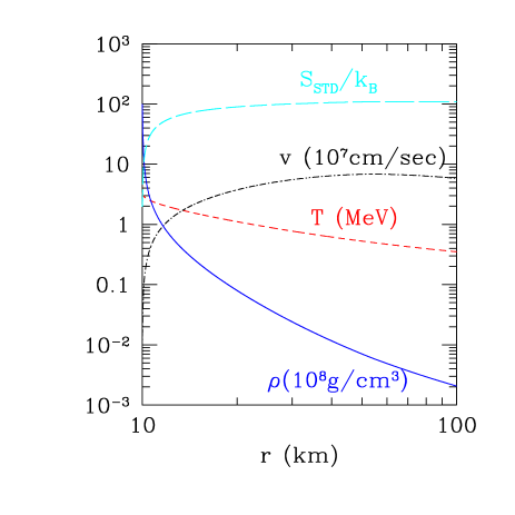
FIG. 1.: Plot of the evolution of the physical quantities as a function of the radial coordinate $r$. They are the entropy per baryon number $S_{\rm STD}/k_{B}$ (long dashed line), the radial velocity $v$ in units of $10^{7}$ cm/sec (dot-dashed line), the temperature $T$ in MeV (dashed line), and the energy density of the matter $\rho$ in $10^{8}{\rm g}$/cm³(solid line).

Now we compute the cases of strong magnetic fields in which $\sqrt{eB}\gg T\gtrsim m_{e}$. Then, it is expected that there exists large anisotropy of the dynamic pressure. For simplicity, it would be adequate for us to consider only the ground state and the next one in the Landau levels (n = 0, 1) because of the Boltzmann suppression of the Fermi distribution. In Fig. 2 we plot the evolution of the entropy in a strong magnetic field. Here we assume that the configuration of the magnetic filed is represented by $B=B_{0}(r/R_{0})^{-m}$, with $B_{0}$ the magnitude of the magnetic field at the surface of the neutron star (= $5\times 10^{16}$ Gauss). The index $m=3$ corresponds to the dipole magnetic field. From the figure we find that the anisotropic dynamic pressure can produce the extra entropy $\Delta S/k_{B}$ which is much larger than the standard value. In Fig. 3 we plot the extra entropy production as a function of the magnetic field at the surface of the neutron star. From the figure, we can see that if the magnetic field is $B\simeq(4-6)\times 10^{16}$ Gauss, we have a large entropy which is required for the successful r-process nucleosynthesis.

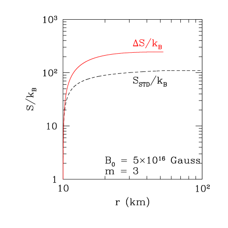
FIG. 2.: Plot of the evolution of the extra increment of the entropy in a strong magnetic filed (solid line). For the sake of comparison, we also plot the standard case in the weak magnetic-field limit $S_{\rm STD}/k_{B}$ (dashed line).

In this study we have investigated the equation of state of electron in strong magnetic fields $B\gtrsim B_{c}$ ($\simeq 4.4\times 10^{13}$ Gauss) and found that it induces the anisotropic dynamic pressure of electron. We have applied the anisotropic dynamic pressure to the r-process nucleosynthesis in core-collapse supernovae. As a result, we obtain a large entropy $S\sim 400k_{B}$ for $B\simeq(4-6)\times 10^{16}$ Gauss. This mechanism of the entropy production might successfully give an account of the observational solar abundances of the heavy nuclei through the r-process nucleosynthesis in the magnetized neutrino wind. Though in this letter we have assumed for simplicity that the magnetic field would not influence the dynamics of the wind, we definitely need more consistent magneto-hydrodynamic models of the wind. That will be discussed in a separate paper [15].

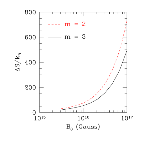
FIG. 3.: Plot of the extra entropy production $\Delta S/k_{B}$ as a function of the magnitude of the magnetic field at the surface of the neutron star. The dashed line represents the case of $m=2$ which corresponds to the configuration which means the flux conservation of the magnetic field. The solid line represents the case of $m=3$ which corresponds to the configuration of the dipole.

REFERENCES

- [1] E. V. Gotthelf and G. Vasisht, New Astronomy 3, 239 (1998), astro-ph/9804025.
- [2] M. G. Baring and Z. K. Harding, Astrophys. J. 547, 929 (2001), astro-ph/0010400.
- [3] R. C. Duncan and C. Thompson, Astrophys. J. Lett. 392, L9 (1992)
- [4] K. Kohri and S. Yamada, astro-ph/0102225.
- [5] S. L. Adler, Annals Phys. 67, 599 (1971).
- [6] M. Chaichian, S. S. Masood, C. Montonen, A. Perez Martinez and H. Perez Rojas, Phys. Rev. Lett. 84, 5261 (2000) [hep-ph/9911218].
- [7] A. Perez Martinez, H. Perez Rojas and H. J. Mosquera Cuesta, hep-ph/0011399.
- [8] R. D. Hoffman, S. E. Woosley and Y. Z. Qian, Astrophys. J. 482, 951 (1997) [astro-ph/9611097].
- [9] C. Itzykson and J. B. Zuber, “Quantum Field Theory,” New York, Usa: Mcgraw-hill (1980) 705 P.(International Series In Pure and Applied Physics).
- [10] Y. Z. Qian and S. E. Woosley, Astrophys. J. 471, 331 (1996) [astro-ph/9611094].
- [11] S. Yamada, Phys. Rev. D 62, 093026 (2000) [astro-ph/0002502].
- [12] A. Holl, V. G. Morozov and G. Ropke, quant-ph/0106004.
- [13] M. Levanda and V Fleurov, cond-mat/0105137.
- [14] H. A. Bethe, Astrophys. J. 412, 192 (1993).
- [15] K. Kohri, S. Nagataki, and S. Yamada, in preparation.