TUM-HEP-422/01 Peculiar effects in the combination of neutrino decay and neutrino oscillations
Talk given at the
ESF-NORDITA WORKSHOP ON NEUTRINO PHYSICS AND COSMOLOGY
June 11-22, 2001, Copenhagen, Denmark

Abstract

In this talk, we will demonstrate some concepts of a simultaneous treatment of neutrino decays and neutrino oscillations in an illustrative manner. This includes topics such as phase coherence discussions and time delay effects of massive supernova neutrinos.

1 Introduction

Neutrino decay in vacuum has often been considered as an alternative to neutrino oscillations (e.g., in [1, 2, 3, 4, 5, 6, 7, 8, 9]). Either neutrino decay only (especially for atmospheric or solar neutrinos) or sequential combinations of neutrino oscillations and decays (especially neutrino oscillations in matter followed by neutrino decay in vacuum: MSW-mediated/MSW-catalyzed solar neutrino decay) have been studied. However, simultaneous neutrino decays and oscillations are also a possible scenario [10]. It involves several quantum field theoretical issues such as phase coherence [10, 11]. In this talk, we will show some peculiarities coming from this sort of discussions, introduced in a quite conceptual manner and illustrated by several examples.

2 Majoron decay as an example

In order to demonstrate several kinematics and coherence issues of a decay model, we choose Majoron decay as an example [12, 13, 14, 15]. Let us assume a generic effective interaction Lagrangian such as

$$\mathcal{L}_{\mathrm{int}}=\underset{i\neq j}{\sum_{i}\sum_{j}}g_{ij}\overline{\nu_{j,L}^{c}}\nu_{i,L}J,$$ (1)

where $J$ is the Majoron field, $\nu_{i}$ are Majorona mass eigenstates, and $g_{ij}$ are the Majoron coupling constants. First of all, we observe that only mass eigenstates and not flavor eigenstates may decay. Second, decay into active as well as sterile neutrinos is, in principle, possible with this type of Lagrangian. Third, we assume the secondary active neutrinos to be, in principle, observable, but the Majorons, to first order, not.

2.1 Re-direction of neutrinos by decay

Re-direction of neutrinos by decay is a purely kinematical effect. Since (at least) a third particle is involved in a decay process, the secondary neutrino may slightly change direction because of energy and momentum conservation. Let us now investigate the consequences for neutrino beams and radially symmetric point sources.

Neutrino beams

Figure 1 shows the geometry of a neutrino beam produced at $S$ and directed towards the detector $D$ with an intermediate decay at $X$.

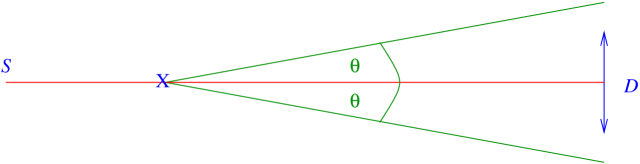
Figure 1: A neutrino beam produced by the source $S$ and detected at the detector $D$, where $D$ is also the area of detection. The decay may happen at $X$, changing the direction of the secondary neutrino by an angle $\theta$.

One can derive from the kinematics of Majoron decay that the angle $\theta$ is limited by a maximum angle $\theta_{\mathrm{max}}$ for $\nu_{i}\rightarrow\nu_{j}$ decay

$$\theta_{\mathrm{max}}=\frac{m_{j}}{2E_{i}}\frac{\Delta m_{ij}^{2}}{m_{j}^{2}},\quad\Delta m_{ij}^{2}\equiv m_{i}^{2}-m_{j}^{2}>0.$$ (2)

The angle $\theta_{\mathrm{max}}$ is determined by the $\frac{m_{j}}{E_{i}}$-dependence for a not too hierarchical mass spectrum. Thus, we obtain for relativistic neutrinos $\theta_{\max}\ll 1$. One can show that active secondary neutrinos are, in principle, observable for accelerator, atmospheric, and reactor neutrinos ($\Delta m_{ij}^{2}\simeq m_{j}^{2}$ assumed) [10].

Radially symmetric neutrino sources

From Fig. 2 we see that for decay of one parent neutrino into exactly one secondary neutrino the overall flux of a radially symmetric neutrino source is conserved.

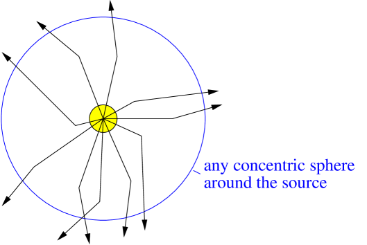
Figure 2: A radially symmetric neutrino source and several paths of neutrinos with one intermediate decay. Drawing any concentric sphere around the source illustrates that the overall flux through any of these spheres is conserved as well as radially symmetric.

Thus, active secondary neutrinos are, in principle, observable for solar and supernova neutrinos. Furthermore, we notice that especially for massive supernova neutrinos, the travel times on different paths may be different even for small angles $\theta_{\mathrm{max}}$. As we will see later, this will modify the time dependence of the signal at the detector.

2.2 Interference effects

In this section, we will study phase coherence in decay processes. Especially, we are interested in the observability of interference effects with intermediate decays between production and detection. Neutrino oscillations of decay products will be one example for such an interference effect.

Neglecting the Majoron field as well as the operators, we know that to first order in the S-matrix expansion

$$d\Gamma\propto\left|\langle out|\int\limits_{-\infty}^{\infty}d^{4}x\mathcal{L}_{\mathrm{int}}|in\rangle\right|^{2},\quad\mathcal{L}_{\mathrm{int}}\sim\sum\limits_{ij}g_{ij}\bar{\nu}_{j}\nu_{i}.$$ (3)

Thus, the interaction destroys an $in$ state and creates an $out$ state by application of the appropriate annihilation and creation operators in the field expansions within the Lagrangian. Let us now assume an incoming and outgoing superposition of mass eigenstates, i.e., active flavor eigenstates (ignoring neutrino propagation):

$$|in\rangle = |\nu_{\alpha}\rangle=\sum\limits_{i}U_{\alpha i}^{*}|\nu_{i}\rangle,$$ (4)

$$|out\rangle = |\nu_{\beta}\rangle=\sum\limits_{j}U_{\beta j}^{*}|\nu_{j}\rangle.$$ (5)

Applying this to Eq. (3) shows that the differential decay rate may indeed contain interference terms $\propto\langle\nu_{j}|S_{ij}|\nu_{i}\rangle^{*}\langle\nu_{l}|S_{kl}|\nu_{k}\rangle$ with $(i,j)\neq(k,l)$, corresponding to interference of different decay channels.

From a different point of view, interference of different decay channels corresponds to coherent summation of amplitudes. This is illustrated in Fig. 3 for the case of Majoron decay.

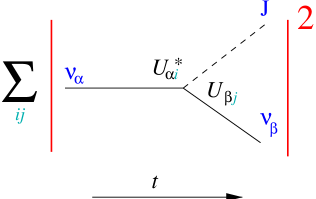
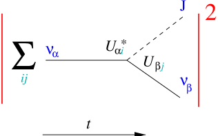
Figure 3: Incoherent (left) and coherent (right) summation of amplitudes for the case of Majoron decay.

Let us compare this to the examples of weak interaction processes shown in Fig. 4.

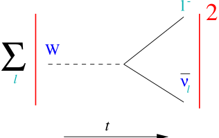
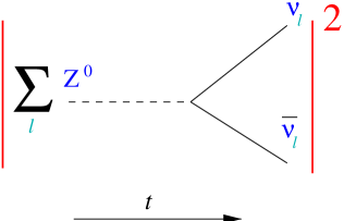
Figure 4: Incoherent (left) and coherent (right) summation of amplitudes for some cases of $W$ (left) and $Z^{0}$ (right) decay.

In the case of $W$ decay, the coherence among the $out$ neutrinos of different flavors is destroyed by the mass differences of the participating leptons corresponding to the different flavors. In other words, the wave packets of the different neutrino flavors do not sufficiently overlap because of the kinematics of the different leptons. Thus, the Feynman diagrams for different flavors need to be summed incoherently. However, in the case of $Z^{0}$ decay, the produced neutrino-antineutrino pairs have small enough mass differences to allow wave packet overlaps of different flavor or mass eigenstates. This means that we need to sum the Feynman diagrams coherently [16].

Comparing $Z^{0}$ decay to Majoron decay, we conclude that interference is not necessarily destroyed in neutrino decay. Thus, depending on the decay scenario, we may have to take into account neutrino oscillations of secondary neutrinos or parent neutrinos, such as illustrated in Fig. 5.

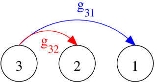
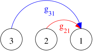
Figure 5: Examples of decay scenarios in which neutrino oscillations of secondary neutrinos (left) or neutrino oscillations of parent neutrinos (right) become, in principle, possible. For these scenarios the Majoron coupling constants shown in the figure need to have non-zero values. The circles correspond to the mass eigenstates $\nu_{3}$, $\nu_{2}$, and $\nu_{1}$, respectively.

2.3 Decay as measurement

Similar to the production and detection processes in neutrino oscillations, neutrino decay acts as a measurement. In general, decay destroys an incoming superposition of mass eigenstates and creates an outgoing one, as it is indicated in Fig. 6.

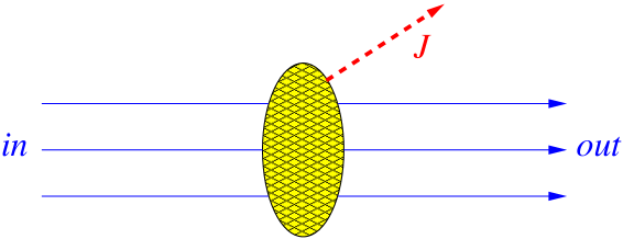
Figure 6: Decay process illustrated, with an $in$ and $out$ superposition of mass eigenstates.

If we can only detect the secondary neutrinos but not the Majorons, we will in many cases (for unchanged quantum numbers and similar energies) not even be able to tell, if there has been a decay between production and detection, or not. However, since there is a third particle involved (the Majoron), these two cases can, in principle, be distinguished. This is equivalent to the fact that Feynman diagrams of different orders do not interfere. Thus, decay acts as a measurement and resets the relative phase among the mass eigenstates in the $out$ state to $0$, similar to the example of $Z^{0}$ decay above. Therefore, for any considered neutrino oscillation (before or after decay) the oscillation phases at the detector depend on the position of the decay. Figure 7 shows the number of neutrinos over the traveling distance for small and large decay rates.

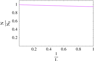
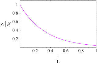
Figure 7: Fraction of undecayed neutrinos $N/N_{0}$ over the fraction of the baseline $l/L$ for small (left) and large (right) decay rates (neutrinos treated as particles). For exponential decay $\propto\exp(-\alpha l/E)$ this corresponds to $\alpha\ll E/L$ (left) and $\alpha\sim E/L$ (right).

For small decay rates, the positions of decay are almost equally spread over the entire traveling distance. Thus, any oscillation phase will be averaged out, similar to the case of production or detection regions larger than the oscillation length. However, for large decay rates more neutrinos will decay in the beginning of the path than at the end. Since the oscillation phases are averaged over all possible decay positions, we may thus expect a net oscillatory effect.

3 Invisible decay products

For decay into unobservable particles, such as sterile decoupled neutrinos, we do not have to take care of secondary neutrinos as well as the type of neutrino source. Therefore, this is the simplest case of neutrino decay. One can show that the transition probability is given by [10]

$$P_{\alpha\beta}^{\rm invisible} = \underbrace{\sum\limits_{ij}\Re J_{ij}^{\alpha\beta}e^{-\Gamma_{ij}}-4\;\underset{i>j}{\sum\limits_{ij}}\Re J_{ij}^{\alpha\beta}\sin^{2}\Delta_{ij}e^{-\Gamma_{ij}}}_{P_{\rm CP\,conserving}}$$ (6)

$$- \underbrace{2\;\underset{i>j}{\sum\limits_{ij}}\Im J_{ij}^{\alpha\beta}\sin 2\Delta_{ij}e^{-\Gamma_{ij}}}_{P_{\rm CP\,violating}}$$

with

$$J_{ij}^{\alpha\beta} \equiv U_{\alpha i}U^{*}_{\alpha j}U^{*}_{\beta i}U_{\beta j},\quad\Delta_{ij}\equiv\frac{\Delta m^{2}_{ij}L}{4E},$$ (7)

$$\Gamma_{ij} \equiv \left(\frac{m_{i}}{\tau_{0,i}}+\frac{m_{j}}{\tau_{0,j}}\right)\frac{L}{2E}=\left(\alpha_{i}+\alpha_{j}\right)\frac{L}{2E}.$$ (8)

Here $\alpha_{i}\equiv m_{i}/\tau_{0,i}$, where $\tau_{0,i}$ is the (rest frame) lifetime of $\nu_{i}$. In Eq. (6) we see that the oscillatory terms are damped by exponentials describing the disappearance of neutrinos into decay products invisible to the detector.

Example: Atmospheric neutrino decay

In order to demonstrate the effects of invisible decay, we may choose a decay scenario similar to the one in Ref. [6] shown in Fig. 8 for atmospheric neutrino decay.

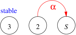
Figure 8: A scenario for atmospheric neutrino decay. Here the mass eigenstate $\nu_{2}$ may decay into a sterile eigenstate, which is not mixing with the active mass eigenstates.

For the parameters we take $\cos^{2}\theta_{23}=0.30$ [6] as well as $\Delta m_{32}^{2}=3.3\cdot 10^{-3}\,\mathrm{eV}^{2}$, since we want to take into account neutrino oscillations in addition to neutrino decay. Figure 9 shows the survival probability $P_{\mu\mu}$ for different decay rates $\alpha$ and sensitivities $L/E$.

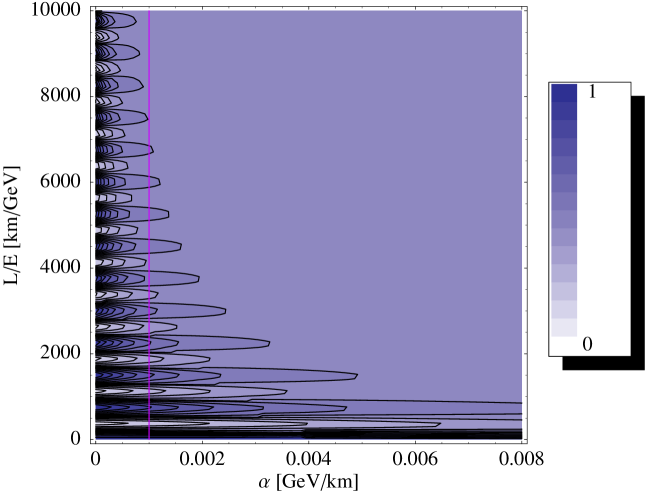
Figure 9: Contour plot of the survival probability $P_{\mu\mu}$ over the decay rate $\alpha$ and the sensitivity $L/E$ (similar plot as in Ref.[10]). The decay scenario used is shown in Fig. 8. For the atmospheric neutrino oscillation parameters we take $\cos^{2}\theta_{23}=0.30$ and $\Delta m_{32}^{2}=3.3\cdot 10^{-3}\,\mathrm{eV}^{2}$.

One can imagine the transition curve between decay and oscillation dominated regions, determined by $\alpha L/E\sim 1$. The purple line in Fig. 9 corresponds to the cut shown in Fig. 10, in which the damping of the oscillation by decay can be clearly seen.

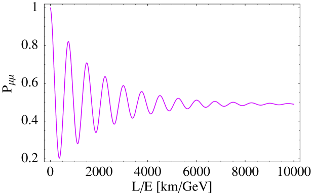
Figure 10: Cut through Fig. 9 at $\alpha=1/1000\,\mathrm{GeV/km}$ at the purple line.

4 Visible decay products in neutrino beams

We showed for the example of Majoron decay that decay into active neutrinos, or sterile neutrinos mixing with active ones, involves more complicated discussions than decay into invisible neutrinos, such as sterile decoupled neutrinos. In this section, we will only give a notion of the results for visible secondary neutrinos in neutrino beams.

Let us define $P_{\alpha\beta}^{i}$ to be the transition probabilities for the flavor transition $\nu_{\alpha}\rightarrow\nu_{\beta}$ with exactly $i$ intermediate decays ($i=0,1,2,\ldots$). In order to calculate the total transition probability, the transition probabilities for different indices $i$ have to be summed over or not. This depends on the ability to distinguish the secondary from the parent neutrinos, i.e., conceptual properties of the detector and the problem. For example, for decay into antiparticles the decay products and the parent neutrinos may have different signatures in the detector. Another example is energy resolution: since neutrinos loose some energy to third particles by decay, the detector may distinguish the parent and secondary neutrinos by its energy resolution.

Assuming that no secondary neutrinos escape detection by kinematics, one can show for the first transition terms $P_{\alpha\beta}^{i}$ that [10]

$$P_{\alpha\beta}^{0} \equiv P_{\alpha\beta}^{\rm invisible},$$ (9)

$$P_{\alpha\beta}^{1} = \underset{i\neq j}{\sum\limits_{ij}}\,\underset{k\neq l}{\sum\limits_{kl}}{L\over E}\frac{\sqrt{\alpha_{ij}\alpha_{kl}}}{\left(\Gamma_{jl}-\Gamma_{ik}\right)^{2}+4\left(\Delta_{ij}+\Delta_{lk}\right)^{2}}$$ (10)

$$\times \bigg{\{}\Re(K_{ijkl}^{\alpha\beta})\left[\left(\Gamma_{jl}-\Gamma_{ik}\right)\left(e^{-\Gamma_{ik}}\cos(2\Delta_{ki})-e^{-\Gamma_{jl}}\cos(2\Delta_{lj})\right)\right.$$

$$- \left.2\left(\Delta_{ij}+\Delta_{lk}\right)\left(e^{-\Gamma_{ik}}\sin(2\Delta_{ki})-e^{-\Gamma_{jl}}\sin(2\Delta_{lj})\right)\right]$$

$$- \Im(K_{ijkl}^{\alpha\beta})\left[\left(\Gamma_{jl}-\Gamma_{ik}\right)\left(e^{-\Gamma_{ik}}\sin(2\Delta_{ki})-e^{-\Gamma_{jl}}\sin(2\Delta_{lj})\right)\right.$$

$$+ \left.2\left(\Delta_{ij}+\Delta_{lk}\right)\left(e^{-\Gamma_{ik}}\cos(2\Delta_{ki})-e^{-\Gamma_{jl}}\cos(2\Delta_{lj})\right)\right]\bigg{\}}$$

$$P_{\alpha\beta}^{2} = \ldots,$$

where $P_{\alpha\beta}^{\rm invisible}$ is given by Eq. (6), $K^{\alpha\beta}_{ijkl}\equiv U^{*}_{\alpha i}U_{\beta j}U_{\alpha k}U_{\beta l}^{*}$ is a generalization of $J^{\alpha\beta}_{ij}$, and $\alpha_{ij}\equiv m_{i}/\tau_{0,ij}$ is the decay rate for the channel $\nu_{i}\rightarrow\nu_{j}$, analogously defined to $\alpha_{i}\equiv m_{i}/\tau_{0,i}\equiv\sum_{j}\alpha_{ij}$.

Example

In order to show the effects for visible decay products, we construct an example with the decay scenario shown in Fig. 11.

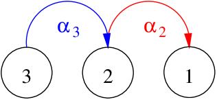
Figure 11: Example for a decay scenario with $m_{3}>m_{2}>m_{1}$.

Let us look at the survival probability of electron neutrinos $P_{ee}$ and ignore higher order decay effects, i.e., only consider $P_{ee}^{0}$ and $P_{ee}^{1}$. For the decay scenario in Fig. 11 one can split up the non-vanishing terms in the sum in $P_{ee}^{1}$ in Eq. (10) into

$$P_{ee}^{1}=P_{ee}^{1,1}+P_{ee}^{1,2}+P_{ee}^{1,\mathrm{int}},$$ (11)

where $P_{ee}^{1,k}$ describes the production of new $\nu_{k}$ by decay and $P_{ee}^{1,\mathrm{int}}$ the interference effects (neutrino oscillations) before or after decay. Figure 12 shows the separated signals and their sum for the parameters in the figure caption.

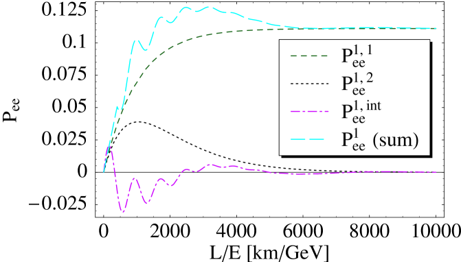
Figure 12: The separated survival probabilities $P_{ee}^{1,k}$ for decay into individual mass eigenstates $\nu_{k}$, the interference probability $P_{ee}^{1,\mathrm{int}}$, as well as the total survival probability with exactly one intermediate decay $P_{ee}^{1}$ (similar plot as in Ref.[10]). Here the decay scenario in Fig. 11 is used with parameter values $\Delta m_{32}^{2}=3.3\cdot 10^{-3}\,\mathrm{eV}^{2}$, $\Delta m_{21}^{2}=5\cdot 10^{-4}\,\mathrm{eV}^{2}$, $\alpha_{2}=1/1000\,\mathrm{GeV/km}$, $\alpha_{3}=1/1100\,\mathrm{GeV/km}$, as well as trimaximal mixing.

The terms $P_{ee}^{1,k}$, describing the production of new mass eigenstates by decay, are exponentially growing in the beginning. For large $L/E$, $P_{ee}^{1,2}$ is falling again because $\nu_{2}$ decays with a larger rate than being produced. The interference term $P_{ee}^{1,\mathrm{int}}$ is basically determined by the two beat frequencies induced by the two $\Delta m^{2}$ involved, i.e., neutrino oscillations before and after decay.

Taking $P_{ee}^{0}$ into account, which describes the survival probability of the neutrinos arriving at the detector without any decay between production and detection, yields the result in Fig. 13.

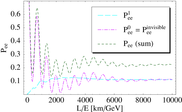
Figure 13: The survival probabilities without intermediate decays $P_{ee}^{0}$ and with one intermediate decay $P_{ee}^{1}$ between production and detection, as well as their sum (similar plot as in Ref.[10]). The parameter values are chosen as given in the caption of Fig. 12.

Note that $P_{ee}^{0}$ and $P_{ee}^{1}$ may only be sensibly added, if the detector cannot distinguish between parent and secondary neutrinos.

5 Decays of supernova neutrinos

In this section, we will focuse on supernova neutrinos. We will show certain properties of supernova neutrino propagation as well as the effects modifying neutrino event rates.

5.1 Issues especially concerning supernova neutrinos

Since a supernova may be approximated as a far-distant point source, we have to incorporate some new concepts (e.g., Refs.[17, 11]):

Time delays of massive neutrinos

For massive neutrinos the velocity of propagation depends on the mass. Even on the direct path $L$, massive neutrinos will be delayed by $\Delta t\simeq Lm^{2}/(2E^{2})$. In addition, re-direction by decay opens the possibility for paths from the supernova to the detector other than the direct path, such as shown in Fig. 14.

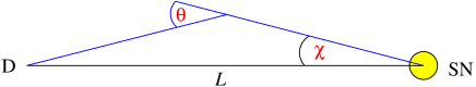
Figure 14: A traveling path from the supernova $SN$ to the detector $D$ different from the direct path along the baseline $L$.

Again, neutrinos will be delayed by an additional time interval, though the change of direction by decay is in many cases quite small.

In order to investigate this effect, let us assume a radially symmetric source producing $N_{\alpha}$ neutrinos of flavor $\nu_{\alpha}$ at $t=-L$, i.e.,

$$\Phi^{\mathrm{tot}}_{\alpha}(t)=\frac{dN_{\alpha}}{dt}=N_{\alpha}\,\delta(t+L),$$ (12)

so that

$$\int\limits_{-\infty}^{\infty}\Phi^{\mathrm{tot}}_{\alpha}(t)dt=N_{\alpha}.$$ (13)

Therefore, for such a source flux massless neutrinos would arrive at $t=0$. Let us further define $\Phi^{D,i}_{\alpha\beta}(t)$ to be the number of neutrinos per time interval at the detector, which are produced as flavor $\nu_{\alpha}$ and detected as flavor $\nu_{\beta}$ with exactly $i$ intermediate decays. This definition is completely analogous to $P^{i}_{\alpha\beta}$, but in addition takes into account the time dependence of the signal.

Loss of coherence because of long baselines

We know from the wave packet treatment of neutrino oscillations that the coherence length of neutrino oscillations with $\Delta m_{ab}^{2}$ is given by [18, 19, 20, 21]

$$L^{\mathrm{coh},I}_{ab}\equiv\frac{4\sqrt{2}\sigma_{x}^{I}E^{2}}{\Delta m_{ab}^{2}}.$$ (14)

Here

$$(\sigma_{x}^{I})^{2}=(\sigma_{x}^{P})^{2}+(\sigma_{x}^{D})^{2}$$ (15)

is the combined wave packet width $\sigma_{x}^{I}$ of the production $P$ and detection $D$ processes. The decay process $X$ can be treated similarly to an intermediate process between production $P$ and detection $D$ by using

$$(\sigma_{x}^{I})^{2}=(\sigma_{x}^{P})^{2}+(\sigma_{x}^{X})^{2}\quad\mathrm{or}\quad(\sigma_{x}^{I})^{2}=(\sigma_{x}^{X})^{2}+(\sigma_{x}^{D})^{2},$$ (16)

depending on what processes we are looking at.

5.2 Dispersion by different neutrino masses

As a first effect, which we illustrate with an example, we demonstrate the propagation of mass eigenstates traveling with different velocities before and after decay because of the different masses of parent and secondary neutrinos. Thus, the arrival time depends on the position of decay. We choose the decay scenario in Fig. 15 and assume incoherent propagation at all times, i.e., the travel distance between any two processes in the problem is much longer than the respective coherence length.

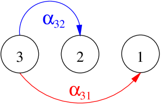
Figure 15: A decay scenario with $m_{3}>m_{2}>m_{1}$ for decay of one mass eigenstate into two different decay channels.

In addition, we ignore effects of different traveling path lengths as well as repeated decays. Figure 16 shows the results for the parameter values given in the figure caption.

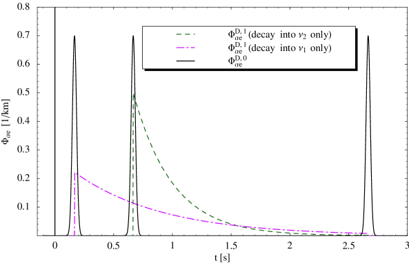
Figure 16: The signals for no intermediate decays between production and detection $\Phi^{D,0}_{\alpha e}$, as well as for one intermediate decay $\Phi^{D,1}_{\alpha e}$, separated into the terms for $\nu_{1}$ and $\nu_{2}$ as decay products (similar plot as in Ref.[11]). In this example, the decay scenario in Fig. 15 with the parameter values $m_{3}=4\,\mathrm{eV}$, $m_{2}=2\,\mathrm{eV}$, $m_{1}=1\,\mathrm{eV}$, $L=10^{22}\,\mathrm{m}\simeq 32\,\mathrm{kpc}$, $E=10\,\mathrm{MeV}$, $\alpha_{32}=\alpha_{31}=E/L$, $N_{\alpha}=9\cdot 10^{5}\,4\pi L^{2}/D$, as well as trimaximal mixing is used. Note that in this example the flavor index $\alpha$ may refer to any flavor.

For no intermediate decays between production and detection, the source pulses are also detected as pulses. For one intermediate decay, the neutrinos travel with the velocity of the heavy parent mass eigenstate before decay and with the velocity of the light secondary mass eigenstate after decay. Thus, one can find the exponential distribution of the decay positions in the time structure of the signal at the detector. This is an effect which may affect or even mimic the signal structure expected from supernova models.

5.3 Dispersion by different traveling path lengths

In this section, we will illustrate the effects of different traveling path lengths with an example. Note that the smaller the maximum re-direction by decay $\theta_{\mathrm{max}}$ is, the smaller the dispersion by time delays on different traveling paths becomes (cf., Fig. 17).

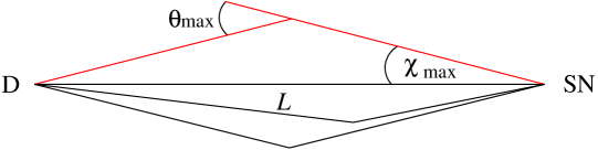
Figure 17: Different paths from the supernova $SN$ to the detector $D$, as well as the path with maximum length by kinematics and geometry (red).

However, there will be dispersion by different neutrino masses even for small $\theta_{\mathrm{max}}$, such as it was shown in the example in Sec. 5.2. We use an example with the decay scenario shown in Fig. 18 and the parameter values from the last example in Sec. 5.2 (cf., caption of Fig. 16).

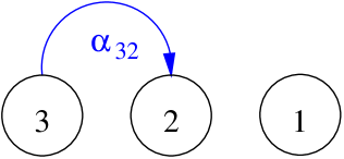
Figure 18: Example for a decay scenario with $m_{3}>m_{2}>m_{1}$.

In addition, we approximate the differential decay rate by its mean

$$\frac{d\Gamma}{d\cos\theta}=\left\{\begin{array}[]{cll}\frac{\Gamma_{\mathrm{tot}}}{1-\cos\tilde{\theta}_{\mathrm{max}}}&\mathrm{for}&\theta\leq\tilde{\theta}_{\mathrm{max}}\\ 0&\mathrm{otherwise}&\end{array}\right.$$ (17)

with an effective $\tilde{\theta}_{\mathrm{max}}\leq\theta_{\mathrm{max}}$. Thus, we may choose $\tilde{\theta}_{\mathrm{max}}$ smaller than the actual $\theta_{\mathrm{max}}$, in order to investigate the dependence on the path lengths. Figure 19 shows the (approximated) signal with one intermediate decay for several values of $\tilde{\theta}_{\mathrm{max}}$.

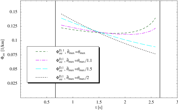
Figure 19: Approximated signal with one intermediate decay for several values of $\tilde{\theta}_{\mathrm{max}}$ defined in the text (similar plot as in Ref.[11]). For the decay scenario we use the one in Fig. 18. The parameter values are chosen such as in the last example in the caption of Fig. 16.

The figure demonstrates that for large $\tilde{\theta}_{\mathrm{max}}$ late time arrivals are favored and early time arrivals suppressed. For small $\tilde{\theta}_{\mathrm{max}}$ we almost observe an exponential behavior such as expected from the last example.

5.4 Early coherent decays

For this effect, we assume the decay rates to be large enough such that the neutrinos are still coherently propagating at the position of decay, but loose coherence between decay and detection. This also implies that all neutrinos decay before detection.

For the decay scenario we need to have simultaneous coupling of two mass eigenstates to the decay product, such as in Fig. 20.

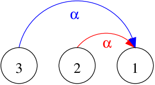
Figure 20: Example for a decay scenario with $m_{3}>m_{2}>m_{1}$ and two decay channels into the same decay product.

In addition, we assume trimaximal mixing. Since it can be shown that the detector can in most cases not resolve the time dependence of the signal, we integrate the flux over time:

$$N_{\alpha\beta}^{D,1}\equiv\int\limits_{-\infty}^{\infty}\Phi_{\alpha\beta}^{D,1}dt.$$ (18)

Moreover, similar to Eq. (11), we define $N_{\mathrm{int}}$ to be the number of neutrinos coming from interference terms in the calculation and $N_{\mathrm{incoh}}$ to be the number of neutrinos coming from incoherent propagation. Figure 21 illustrates that for small $\Delta m_{32}^{2}\ll\alpha$ interference effects become most important.

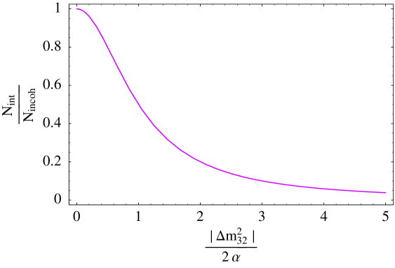
Figure 21: The ratio of neutrinos coming from the calculation of interference terms $N_{\mathrm{int}}$ to the number of neutrinos coming from incoherent propagation $N_{\mathrm{incoh}}$. This ratio is plotted over the ratio of $\Delta m_{32}^{2}$, which causes the interference terms, to the decay rate $\alpha$. For the calculation trimaximal mixing as well as the decay scenario in Fig. 20 is assumed.

For larger $\Delta m_{32}^{2}$ more and more oscillations take place until the neutrinos decay and thus the oscillation phases at the position of decay are more and more averaged out over all possible decay positions. Note that we may observe an interference effect, even if only one stable neutrino arrives at the detector.

6 Summary

So far, parameters have only been fitted for neutrino oscillations or special neutrino decay scenarios. However, fitting all oscillation and decay parameters may produce new solutions. Furthermore, decay effects for supernova neutrinos have been ignored. Taking them into account may alter or even mimic the signals expected from supernova models. Finally, supernova neutrino observations have only indicated that at least one mass eigenstate is stable. Nevertheless, interference phenomena may have to be taken into account, even if only one stable mass eigenstate arrives at the detector. Since non-zero values for neutrino masses imply, in principle, not only neutrino oscillations, but also neutrino decay, we conclude that neutrino decay should be incorporated into the general neutrino oscillation discussion.

Acknowledgements

The author would like to thank Manfred Lindner and Tommy Ohlsson for useful discussions and comments, Jörn Kersten and Tommy Ohlsson for proofreading the manuscript, and Lars Bergström, Steen Hannestad, Kimmo Kainulainen, and Georg Raffelt for organizing the workshop.

This work was supported by ESF (“European Science Foundation”), NORDITA, the “Studienstiftung des deutschen Volkes” (German National Merit Foundation), and the “Sonderforschungsbereich 375 für Astro-Teilchenphysik der Deutschen Forschungsgemeinschaft”.

References

- [1] S. Pakvasa and K. Tennakone, Phys. Rev. Lett. 28 (1972) 1415.
- [2] J.N. Bahcall, N. Cabibbo and A. Yahil, Phys. Rev. Lett. 28 (1972) 316.
- [3] R.S. Raghavan, X.G. He and S. Pakvasa, Phys. Rev. D38 (1988) 1317.
- [4] A. Acker, A. Joshipura and S. Pakvasa, Phys. Lett. B285 (1992) 371.
- [5] V. Barger et al., Phys. Rev. Lett. 82 (1999) 2640, astro-ph/9810121.
- [6] V. Barger et al., Phys. Lett. B462 (1999) 109, hep-ph/9907421.
- [7] G.L. Fogli et al., Phys. Rev. D59 (1999) 117303, hep-ph/9902267.
- [8] S. Choubey, S. Goswami and D. Majumdar, Phys. Lett. B484 (2000) 73, hep-ph/0004193.
- [9] A. Bandyopadhyay, S. Choubey and S. Goswami, hep-ph/0101273.
- [10] M. Lindner, T. Ohlsson and W. Winter, Nucl. Phys. B (to be published), hep-ph/0103170.
- [11] M. Lindner, T. Ohlsson and W. Winter, (2001), astro-ph/0105309.
- [12] G.T. Zatsepin and A.Y. Smirnov, Yad. Fiz. 28 (1978) 1569, [Sov. J. Nucl. Phys. 28 (1978) 807].
- [13] Y. Chikashige, R.N. Mohapatra and R.D. Peccei, Phys. Rev. Lett. 45 (1980) 1926.
- [14] G.B. Gelmini and M. Roncadelli, Phys. Lett. B99 (1981) 411.
- [15] S. Pakvasa, hep-ph/0004077.
- [16] A.Y. Smirnov and G.T. Zatsepin, Mod. Phys. Lett. A7 (1992) 1272.
- [17] Y. Aharonov, F.T. Avignone and S. Nussinov, Phys. Lett. B200 (1988) 122.
- [18] C. Giunti, C.W. Kim and U.W. Lee, Phys. Rev. D44 (1991) 3635.
- [19] C. Giunti and C.W. Kim, Phys. Rev. D58 (1998) 017301, hep-ph/9711363.
- [20] W. Grimus, P. Stockinger and S. Mohanty, Phys. Rev. D59 (1999) 013011, hep-ph/9807442.
- [21] C.Y. Cardall, Phys. Rev. D61 (2000) 073006, hep-ph/9909332.