1 Introduction

One of the main goals of the next generation of colliders will be to explore the Higgs sector phenomenology. The simplest candidates for Higgs sector physics beyond the standard model (SM) are the two Higgs doublet models (2HDM) [1], and, among these, the leading one is provided by the minimal supersymmetric standard model (MSSM) [2]. This requires a Higgs sector called of type II, where one of the Higgs doublets couples to the toplike quarks and the other to the bottomlike quarks. The basic differences between the MSSM and a general 2HDM of type II (2HDMII) depend, first, on the supersymmetric (SUSY) sector, which is obviously absent in the 2HDMII, and, second, on the different values of the Higgs boson self-couplings. In the MSSM, because of the underlying supersymmetry, these couplings are fixed in terms of the electroweak gauge couplings.

In all these models, the physical Higgs boson spectrum consists of two neutral CP-even Higgs bosons $h^{o}$ and $H^{o}$, one CP-odd Higgs boson $A^{o}$, and two charged Higgs bosons $H^{\pm}$ [1]. The tree-level parameters are the Higgs boson masses $m_{h^{o}}$, $m_{H^{o}}$, $m_{A^{o}}$, and $m_{H^{\pm}}$, the mixing angle in the CP-even neutral sector, $\alpha$, and the ratio of the vacuum expectation values of the two Higgs doublets, $\tan\beta=v_{2}/v_{1}$. In the MSSM, due to supersymmetry, these can be written in terms of just two free parameters, which are usually chosen as $m_{A^{o}}$ and $\tan\beta$. The Higgs boson masses are therefore not independent parameters in the MSSM, as they are in a general 2HDMII. Once the radiative corrections are included these tree-level mass relations are significantly modified, but there still remains a clear pattern for the Higgs boson masses in terms of the MSSM parameters [3, 4]. Hence, if all these masses could be measured with good precision the mass pattern itself would be a first indirect indication of their SUSY origin.

The most striking prediction of the MSSM is that the lightest Higgs boson mass lies below 130-135 GeV, within the reach of present and next generation colliders, the Fermilab Tevatron [5] and the CERN Large Hadron Collider (LHC) [6]. The properties of this Higgs boson $h^{o}$, however, are very similar to those of the SM Higgs particle in the so-called decoupling regime where $m_{A^{o}}\gg m_{Z}$ [7]. For the relevant $h^{o}$ production processes and decay channels at the LHC, this decoupling already occurs, in practice, at $m_{A^{o}}$ values not far from the electroweak scale $m_{\rm EW}$. For instance, the difference in the width of the main decay $h^{o}\rightarrow b\bar{b}$, from the SM value is less than $10\%$ for $m_{A^{o}}>350\,{\rm GeV}$ and $2<\tan\beta<50$. There is just one region, corresponding to low $m_{A^{o}}$ and large $\tan\beta$ values, where the pattern of $h^{o}$ branching ratios significantly differs from the SM one. It is because in this region the dominant decays to $b\bar{b}$ pairs and to $\tau^{+}\tau^{-}$ pairs are enhanced and, as a consequence, the subdominant channels are significantly suppressed. Thus, for most of the ($m_{A^{o}}$, $\tan\beta$) parameter space it seems difficult to disentangle the nonstandard nature of $h^{o}$ and, in order to decide on its SUSY origin, one must consider in addition the phenomenology of the other Higgs particles (for a review see, for instance, [8]). The relevant question then becomes one of finding SUSY signals by looking into $h^{o}$, $H^{o}$, $A^{o}$ and $H^{\pm}$ production and decays at colliders, and of distinguishing these signals from those of a general 2HDMII. Obviously, if the SUSY particles are within the reach of the LHC and/or the Tevatron, the priority is to look for their direct production. However, it may well happen that these turn out to be too heavy to be produced directly. In that case one will have to look for indirect SUSY signals via their contributions as virtual intermediate states in standard processes, in much the same way as was done in the past at the CERN $e^{+}e^{-}$ collider LEP for indirect effects from top and Higgs particles in precision observables. We are particularly interested here in their contributions to the radiative corrections involved in Higgs physics.

In this work, we consider a scenario where some or all of the Higgs particles have been discovered and their masses and branching ratios have been measured, but the SUSY particles have not shown up yet. We will study optimal strategies to look for indirect SUSY signals via their radiative corrections in Higgs boson decays [9, 10, 11, 12, 13, 14, 15]. Since it is known that there are specific decay processes where some SUSY radiative corrections do not decouple, even in the case of a extremely heavy SUSY spectrum  [16, 17, 18, 21, 19, 20, 22, 23], we will concentrate on these particular channels. This nondecoupling behavior is a genuine part of Higgs sector physics and has not been found yet in other MSSM sectors, such as, for instance, electroweak gauge boson physics [24]. The nondecoupling processes we consider here are the Higgs boson decay channels into quark pairs, and more specifically we will concentrate on those that are enhanced at large $\tan\beta$ values: $h^{o}\rightarrow b\bar{b}$, $H^{o}\rightarrow b\bar{b}$, $A^{o}\rightarrow b\bar{b}$ [9, 17, 18, 10, 20, 16, 21] and $H^{+}\rightarrow t\bar{b}$ [11, 12, 19, 13, 20, 22]. We will also analyze the top quark decay channel $t\rightarrow H^{+}b$ [14, 15] which is complementary to the $H^{+}\rightarrow t\bar{b}$ decay for low $m_{A^{o}}$ values. We will focus, in particular, on the SUSY QCD corrections from third-generation squarks, $\tilde{q}$, and gluinos, $\tilde{g}$, which are the dominant SUSY radiative corrections for most of the MSSM parameter space and are numerically sizable [9, 10, 11, 12, 14]. For instance, in $H^{+}\rightarrow t\bar{b}$ they can be as large as $60\%$ and of either sign for quasidegenerate gluinos and squarks of mass 1 TeV and $\tan\beta=50$. These nondecoupling corrections were derived recently in [23] for all the Higgs boson decay channels into all possible quark pairs, and analyzed in more detail for the $h^{o}\rightarrow b\bar{b}$ [16, 17, 18, 20, 21] and $H^{+}\rightarrow t\bar{b}$  [19, 20, 22] channels. For nearly degenerate gluinos and squarks these SUSY QCD corrections, to one-loop level, can be generically written as $\Gamma=\Gamma^{0}(1+\alpha_{S}\frac{\mu M_{\tilde{g}}}{M_{\rm SUSY}^{2}}K)$, where $\Gamma^{0}$ is the corresponding partial decay width without the SUSY QCD contribution, $\alpha_{S}$ is the strong coupling constant, $\mu$ is the bilinear Higgs boson MSSM parameter, $M_{\tilde{g}}$ is the gluino mass, $M_{\rm SUSY}$ is a common generic SUSY mass characterizing the squark masses, and $K$ is a function of $\beta$ and $\alpha$ that depends on the specific channel [23]. The nondecoupling behavior is seen here as a nonvanishing contribution to the partial width of order ${\cal O}(\alpha_{S}K)$, which is present even in the limit of a heavy SUSY spectrum where $|\mu|\sim M_{\tilde{g}}\sim M_{\rm SUSY}\gg m_{\rm EW}$. These corrections are known to be particularly relevant for the $h^{o},H^{o},A^{o}\rightarrow b\bar{b}$, $H^{+}\rightarrow t\bar{b}$, and $t\rightarrow H^{+}b$ decays, because it is precisely in these channels that the function $K$ grows linearly with $\tan\beta$ and can provide sizable contributions for the interesting large $\tan\beta$ region. It is worth mentioning that the SUSY electroweak (SUSY EW) corrections may also be relevant in particular regions of the MSSM parameter space [9, 13, 15]. In the large $\tan\beta$ regime and for quasidegenerate squarks, neutralinos, and charginos, these are known to behave as $\sim(\frac{h_{t}}{4\pi})^{2}\frac{\mu A_{t}}{M_{\rm SUSY}^{2}}\tan\beta$, where $M_{\rm SUSY}$ is the common generic mass for squarks, neutralinos, and charginos, $h_{t}$ is the tree-level top quark Yukawa coupling, $h_{t}=\frac{gm_{t}}{{\sqrt{2}}m_{W}\sin\beta}$, and $A_{t}$ is the top quark trilinear coupling [16, 17, 18]. For small or moderate $A_{t}$ values and a heavy SUSY spectrum, these SUSY EW corrections are considerably smaller than the SUSY QCD ones and can be ignored, but for very large $A_{t}$ values, $|A_{t}|\sim|\mu|\sim M_{\rm SUSY}\gg m_{\rm EW}$, these SUSY EW corrections do not decouple either and, depending on their sign, can increase or decrease the nondecoupling effect of the SUSY QCD corrections.

In order to select optimal observables to look for these indirect SUSY QCD signals we require of them, first, to be measurable at the Tevatron [5], LHC [6], and/or the next generation linear colliders;. second, to be most sensitive to the mentioned SUSY QCD corrections; and, third, to have the minimal theoretical and experimental uncertainties. We propose and analyze here a set of observables that satisfy all these conditions. These are the ratios of the branching ratios of the Higgs boson decays into third-generation quarks to the branching ratios of this same Higgs boson into third-generation leptons. We will show that these ratios can be considered optimal observables because of the following reasons:
$\bullet$ The SUSY QCD nondecoupling corrections contribute just to the numerator, that is, to quark decays and not to lepton decays. The first will be considered as the search channel, the second as the control channel.
$\bullet$ These corrections are maximized at large $\tan\beta$ and are sizable enough to be measurable.
$\bullet$ The production uncertainties are minimized in ratios.
$\bullet$ They will be experimentally accessible at the LHC or Tevatron.
$\bullet$ They will allow one to distinguish the MSSM Higgs sector from a general 2HDMII.

The paper is organized as follows. Section 2 is devoted to an experimental overview of Higgs particle searches at the Tevatron and LHC. The relevant regions in the $(m_{A^{o}},\tan\beta)$ plane are briefly reviewed. In Section 3 the set of optimal observables is presented and analyzed in full detail. The leading contributions from tree-level and standard QCD corrections to these observables are also studied and their theoretical uncertainties estimated. The explicit formulas for nondecoupling SUSY QCD corrections from heavy squarks and gluinos are presented. A discussion of the relevance of the SUSY EW corrections is also contained in Section 3. A comparison between a general 2HDMII and the MSSM is also included. The numerical results for the proposed observables and a discussion as a function of the MSSM parameters are presented in Section 4. Finally, the conclusions are summarized in Section 5.

2 Experimental overview

In this section we turn to the perspectives of the experimental measurement itself. We focus on the next hadron colliders: the Tevatron and LHC. From this point of view, a measurement of the SUSY radiative corrections in Higgs physics is the next step in the problem of discovering a signal of the existence of one or several Higgs particles. Only after a discovery, but immediately after, will the question of what is the underlying structure of the Higgs sector be raised. As we have said, this is the principal motivation of our study.

The discovery reach problem has been studied carefully and extensively by several working groups, both for the Tevatron Run 2 [5] and for the LHC [6]. In particular, the searches for SM or MSSM Higgs bosons were used as benchmark channels during the design of the ATLAS and CMS detectors.

Following the results of these studies, one learns that for values of $\mbox{tan}~{}\beta$ large enough so that the corrections are sizable, there are three regions in the ($m_{A^{o}}$, $\mbox{tan}~{}\beta$) plane of phenomenological interest.

The first is the region of large values of $\mbox{tan}~{}\beta$ (say $\gtrsim 10$), and low $m_{A^{o}}$ (say $m_{A}\lesssim 120$ GeV). Here several production processes grow with $\mbox{tan}^{2}~{}\beta$, and the corresponding cross sections are much larger than the typical SM ones. One example is the associated production of a CP-odd boson $A^{o}$ and bottom quarks: $gg(q\bar{q})\to b\bar{b}A^{o}$. In this region of the MSSM, the lighter CP-even boson $h^{o}$ has essentially the same couplings and mass (within 5%) as the $A^{o}$, effectively doubling the production cross section [1]. The heavier CP-even boson $H^{o}$ has SM bosonlike couplings, and its production rates are considerably smaller. In turn, the charged Higgs boson $H^{\pm}$ is lighter than the top quark, and $t\to bH^{+}$ happens in a sizable part of the top quark decays.

With such large cross sections and relatively small masses this has been the main region examined at the Tevatron during Run 1. In fact, the Collider Detector at Fermilab (CDF) Collaboration has already searched for associated production of $b\bar{b}A^{o}(h^{o})$, where $A^{o}(h^{o})\to b\bar{b}$ [27], or $A^{o}(h^{o})\to\tau^{+}\tau^{-}$ [28], excluding a part of the ($m_{A^{o}}$, $\tan\beta$) plane. Also, the CDF and D0 Collaborations have excluded a part of the MSSM parameter space corresponding to unobserved decays $t\to bH^{+}$, with $H^{+}\to\tau^{+}\nu$  [29], more specifically, the region where $\frac{\Gamma(t\to H^{+}b)}{\Gamma(t\to W^{+}b)}\gtrsim 1$. It is clear that the search will continue in Run 2, and a discovery is possible before the start of the LHC [5].

The first analysis takes advantage of both the large cross section (${\cal O}$(1-100 pb)) and large $\mbox{B}(A^{o}\to b\bar{b})\sim 90\%$. The experimental signature is four jets with at least three of them $b$ tagged. This channel has also the advantage that it allows the reconstruction of $m_{A^{o}}$ and, once this mass is known, the production rate gives an idea of the size of $\mbox{tan}~{}\beta$. On the other hand, as in any search in a purely hadronic channel, the QCD background has to be properly understood. Systematic errors at the $20-30\%$ level are not infrequent [27].

In contrast, the channel $A^{o}\to\tau^{+}\tau^{-}$, has to overcome a relatively smaller branching ratio ($\sim$10%). However, the electroweak background $Z(\to\tau^{+}\tau^{-})+{\rm jets}$ is considerably less dangerous [28].

If an $A^{o}$ signal were found in these analyses, the corresponding ratio of $b\bar{b}$ to $\tau^{+}\tau^{-}$ events would be a direct test of the SUSY QCD corrections.

A possible signal in the charged Higgs boson channel could also be useful [15]. In this case, it also happens that the SUSY QCD corrections do not decouple in the $t\to bH^{+}$ decay but they do decouple in the standard channel, $t\to bW^{+}$ [26, 30]. This is the reason why $\Gamma(t\to bW^{+})$ is considered now as the corresponding control width. The problem in this case is that the tree-level prediction changes rapidly with $m_{H^{+}}$ and $\mbox{tan}~{}\beta$. On the other hand, the accuracy in the experimental reconstruction of $m_{H^{+}}$ in the decay $H^{+}\to\tau^{+}\nu$ is limited, and this channel by itself does not provide information about $\mbox{tan}~{}\beta$. It should be pointed out that the LHC experiments will be able to explore this channel very efficiently.

The second region of interest still has large $\mbox{tan}~{}\beta$, but $140$ GeV $\lesssim m_{A^{o}}\lesssim 500$ GeV. With such large masses this can be considered the genuine search zone of the LHC experiments [6]. In this zone, the heavier CP-even boson $H^{o}$ has similar couplings and mass than the $A^{o}$ boson, again doubling the cross section of the process $gg(q\bar{q})\to b\bar{b}A^{o}(H^{o})$ (${\cal O}$(10-1000 pb)). Now the light CP-even Higgs boson $h^{o}$ behaves like the one in the SM with $m_{h^{o}}\sim 110-130$ GeV (the precise mass value depends on the choice of the MSSM parameters). In this region, the mass of the charged Higgs boson is either very close to $m_{t}$ and $\mbox{B}(t\to bH^{+})$ is negligible, or $m_{H^{+}}>m_{t}$ and $t\to bH^{+}$ is directly forbidden. Then, the main possibility of producing charged Higgs bosons is in the process $gg(q\bar{q})\to b\bar{t}H^{+}$. Again, this cross section grows approximately (at large enough $\tan\beta$) with $\mbox{tan}^{2}~{}\beta$.

The main possibility of the Tevatron here would be to detect the SM-like boson $h$ in the associated production $q\bar{q}\to W(Z)\ h^{o}$ and $h^{o}\to b\bar{b}$. Also, the analysis of the ratio $(A^{o}\to b\bar{b})/(A^{o}\to\tau^{+}\tau^{-})$ can be extended, but only for relatively small values of $m_{A^{o}}$ and very large values of $\mbox{tan}~{}\beta$ [5].

With respect to these last channels at the LHC, the challenge will be to detect the decay $A^{o}(H^{o})\to b\bar{b}$ in events with four $b$ jets. Studies have shown that to control the QCD background will be very difficult. In contrast, it will be possible to measure the decay $A^{o}(H^{o})\to\tau^{+}\tau^{-}$ and even $A^{o}(H^{o})\to\mu^{+}\mu^{-}$. Both channels are leptonic, and therefore do not allow an estimation of the SUSY QCD corrections. However, they will provide good measurements of $m_{A^{o}}$ and $\mbox{tan}~{}\beta$, which can be used in addition to other analyses (say, $H^{+}\to\tau^{+}\nu$). Current studies for the LHC [6] indicate that values of $\Delta m_{A^{o}}/m_{A^{o}}$ better than $\sim 1\%$ and of $\Delta\tan\beta/\tan\beta$ better than $\sim 12\%$ ( if $\tan\beta>10$) can be reached.

In the case that $m_{H^{+}}>m_{t}+m_{b}$, the decay channel $H^{+}\to t\bar{b}$ opens and can be used not only to complement the decay $H^{+}\to\tau^{+}\nu$, but also to provide an independent estimation of $m_{A^{o}}$ (in the frame of the MSSM) and $\mbox{tan}~{}\beta$.

Finally, we mention the very interesting region with $m_{A^{o}}\gtrsim 140$ GeV and intermediate $3\lesssim\mbox{tan}~{}\beta\lesssim 10$. At the LHC this zone is called the “hole” because the only Higgs particle accessible is the SM-like one. Here the main question would be not only to discriminate the MSSM from a more general 2HDM sector, but to know if there is something beyond the plain SM.

We will see in the next sections how the SUSY QCD corrections can be used for that matter.

3 Optimal observables

In this section we present the set of observables that are the most sensitive to the nondecoupling SUSY QCD corrections.

Since we are looking for indirect signals of SUSY in an experimental scenario described by the discovery of Higgs particles, with masses following the MSSM pattern, and where the SUSY particles are too heavy to be produced in colliders, we will search for observables with very specific conditions. From the theoretical point of view the requirements are the following:

• In order to discriminate between the MSSM and a nonsupersymmetric 2HDMII, we need observables with different predictions for these two models.

• These predictions should be distinguishable even in the case of a very heavy SUSY spectrum.

• The theoretical uncertainties must be minimized. Some specific ratios of branching ratios will cancel these uncertainties either totally or partially. In particular, we wish the $\tan\beta$ and $\alpha$ dependence to appear just in the correction, but not in the lowest order contribution.

On the other hand, the experimental requirements are the following:

• A control channel is needed in order to eliminate systematic errors, so that ratios of event rates are better than event rates themselves.

• The corrections to the observables should be sizable in the large $\tan\beta$ regime, since the relevant Higgs particle production cross sections grow with this parameter, such that we have better statistics for larger values of $\tan\beta$.

• There should be good identification of the final state particles.

• Experimental uncertainties from Higgs particle production must be minimized. These will cancel in some specific ratios of events from Higgs particle decays.

• The expected accuracy at the LHC and Tevatron for these observables should be good enough that the deviation produced by the corrections becomes apparent. In particular, the size of the SUSY QCD corrections must be larger than the expected error bars.

We propose the following set of optimal observables, which satisfy the previous theoretical and experimental requirements:

In addition, we consider the following ratio:

$$O_{t}\equiv\frac{B(t\to H^{+}b)}{B(t\to W^{+}b)},$$ (2)

which complements the charged Higgs boson observable in the low $m_{A^{o}}$ region. The predictions for these observables at the tree level are the same for any general 2HDMII, and in particular for the MSSM. These are

where

As a general remark, the differences in the predictions from the various models for all these observables come in the corrections beyond the tree level and will be discussed in the following subsections. In particular, it is interesting to emphasize that the predictions for the neutral Higgs boson observables at the tree level are independent of $\tan\beta$ and $\alpha$. The charged Higgs boson observable depends on $\tan\beta$, but this dependence is very mild in the large $\tan\beta$ region. Therefore, these observables are especially sensitive to any extra contribution growing with $\tan\beta$. In the top quark decay observable, however, the tree level prediction goes as $\tan^{2}\beta$, for large $\tan\beta$, and it will be more difficult to disentangle the mentioned contributions. Other analyses of the observables for the neutral channels in the large $\tan\beta$ limit and in the zero external momentum approximation can be found in [18, 31]. The neutral channel case with Higgs boson mass corrections included has been analyzed in [17].

3.1 Supersymmetric QCD contributions

The nondecoupling SUSY QCD contributions to these observables in the MSSM can be easily derived from the results for the effective Yukawa interactions of the Higgs sector with top and bottom quarks. These have been recently obtained at one-loop level, for arbitrary $\tan\beta$, and by a functional integration of bottom and top squarks and gluinos in [23]. For nearly degenerate heavy squarks and gluinos, these corrections can be written as

Here, $\mu$ and $M_{\tilde{g}}$ are the MSSM bilinear parameter and the gluino mass, respectively. $M_{\rm SUSY}$ is the common SUSY mass for squarks and gluinos ($M_{\rm SUSY}\sim M_{\tilde{q}}\sim M_{\tilde{g}}$) and $\alpha_{S}$ is the strong coupling constant evaluated at the corresponding decaying particle mass. The leading terms $O^{o}$ refer to the value of the observables without the SUSY particle contributions and will be discussed in subsection 3.3. These formulas are for heavy squarks and gluinos, that is, for large $M_{\rm SUSY}$, and are valid for all $\tan\beta$ and $m_{A^{o}}$ values. Corrections to the previous formulas are either of higher order in $\alpha_{S}$ or suppressed by higher inverse powers of the heavy SUSY masses $M_{\rm SUSY}$ and, for the present analysis, can be safely ignored.

From a first look at eq.(LABEL:eq.exprobs) one sees clearly that the observables have different predictions within the MSSM and in a general 2HDMII, since the former includes the SUSY QCD corrections, which do not exist in the latter. This main difference comes from the nondecoupling behavior of the SUSY QCD corrections in the Higgs boson decays into quarks (and in the top quark decay into charged Higgs bosons), which is relevant even for a very heavy SUSY spectrum, such that $M_{\tilde{g}}\sim|\mu|\sim M_{\rm SUSY}\gg m_{\rm EW}$. Notice also that, as mentioned before, these SUSY QCD contributions grow linearly with $\tan\beta$ so we expect sizable corrections for large $\tan\beta$.

There are two limiting situations that are worth mentioning: the large $m_{A^{o}}$ limit $m_{A^{o}}\gg m_{Z}$, and the large $\tan\beta$ limit $\tan\beta\gg 1$. In the former limit, $\cot\alpha$ approaches $-\tan\beta$ (correspondingly, $\tan\alpha\rightarrow-\cot\beta$) and, as can be seen in eq.(LABEL:eq.exprobs), the SUSY QCD correction decouples in $O_{h^{o}}$. The other observables get exactly the same nondecoupling correction, proportional to $(\tan\beta+\cot\beta)$. In addition, in this limit, the $H^{o}$ and $H^{+}$ masses approach the large $A^{o}$ mass. The leading contribution $O^{o}_{h^{o}}$ approaches the SM prediction and, therefore, as noted before, the situation cannot be distinguished from the SM case. In the large $\tan\beta$ limit, the corrections do not decouple in any channel, they are all proportional to $\tan\beta$ and all have the same sign. The universal character of the corrections will be very useful in a global analysis, because it will yield strongly correlated signals in all the channels.

3.2 Other nondecoupling contributions in the minimal supersymmetric standard model

It is well known that, in particular regions of the MSSM parameter space the radiative corrections from the SUSY EW sector can also be relevant in the decays of the Higgs bosons and top quark that we are considering here [9, 13, 15]. These SUSY EW corrections are largely dominated by the contributions with charginos or neutralinos and third-generation sfermions in the loops; the contributions from the Higgs sector being negligible. For instance, in the $H^{+}\rightarrow t\bar{b}$ case with $m_{H^{+}}=250$ GeV and for light top and bottom squarks and light charginos and neutralinos, $M_{\tilde{q}},M_{\tilde{\chi}}\leq 200$ GeV, they contribute as much as $\pm 20\%$ with respect to the tree level width, whereas the SUSY QCD loops induced by squarks and gluinos are by far the leading SUSY effects and give a contribution larger than $\pm 50\%$ [13]. These SUSY EW corrections can only be competitive with the SUSY QCD ones in the particular region of the SUSY parameter space where $\tan\beta$ is very large ($\tan\beta>20$), the bottom squarks are very heavy ($M_{\tilde{b}}>300$ GeV), and the top squarks and charginos are relatively light ($M_{\tilde{t}},M_{\tilde{\chi}}\sim 100-200$ GeV). For this particular choice, the total SUSY correction remains around (30-50)$\%$ of the tree level width, with at most half of it of SUSY EW origin [13].

For our present assumption of a very heavy SUSY spectrum with nearly degenerate SUSY particle masses ($M_{\tilde{t}}\sim M_{\tilde{b}}\sim M_{\tilde{g}}\sim M_{\tilde{\chi}}\sim|\mu|\sim M_{SUSY}\gg m_{EW}$) the SUSY QCD corrections provide by far the dominant contribution to the one-loop MSSM correction. However, it is worth analyzing in more detail the SUSY EW corrections, which are known to provide extra non-decoupling contributions. These nondecoupling SUSY EW effects have been estimated in the literature just in the large $\tan\beta\gg 1$ regime and by means of an effective Lagrangian formalism, which works in the zero external momentum approximation [16, 18, 19]. In this approach, the potentially large $\tan\beta$ enhanced SUSY corrections to the Higgs boson-quark-quark Yukawa couplings are induced via the quark mass corrections. In particular, the expression for the bottom quark Yukawa coupling, at the one-loop level and in the large $\tan\beta$ limit, is [16, 19, 20]

$$h_{b}=\frac{m_{b}}{v}\tan\beta(1-\Delta m_{b}),$$ (6)

where $m_{b}$ is the on-shell pole bottom quark mass, $v=174$ GeV, and the $\tan\beta$ enhanced radiative corrections are encoded in

$$\Delta m_{b}=\Delta m_{b}^{SQCD}+\Delta m_{b}^{SEW},$$ (7)

where $\Delta m_{b}^{SQCD}$ and $\Delta m_{b}^{SEW}$ refer to the bottom quark mass corrections from the SUSY QCD and SUSY EW sectors, respectively. $\Delta m_{b}^{SQCD}$ is dominated by the bottom squark-gluino loops, and to leading order in the strong coupling is [4, 16, 19, 20]:

$$\Delta m_{b}^{SQCD}=\frac{2\alpha_{s}}{3\pi}M_{\tilde{g}}\mu\tan\beta I(M_{\tilde{b}_{1}},M_{\tilde{b}_{2}},M_{\tilde{g}}).$$ (8)

For sizable values of the soft trilinear coupling $A_{t}$, $\Delta m_{b}^{SEW}$ is dominated by the top squark-chargino loops and more precisely by the top squark-charged higgsino contribution. By neglecting the bino effects, which have been found to be numerically insignificant, the SUSY EW mass correction to leading order in the top quark Yukawa coupling and the electroweak gauge coupling is [4, 16, 19],

where $M_{2}$ is the SUSY soft breaking chargino mass parameter and $c_{q}=\cos\theta_{\tilde{q}}$, $s_{q}=\sin\theta_{\tilde{q}}$, with $\theta_{\tilde{q}}$ the $\tilde{q}$ mixing angle. The one-loop integrals in $\Delta m_{b}^{SQCD}$ and $\Delta m_{b}^{SEW}$ are defined by,

$$I(m_{1},m_{2},m_{3})=\frac{m_{1}^{2}m_{2}^{2}log\frac{m_{1}^{2}}{m_{2}^{2}}+m_{2}^{2}m_{3}^{2}log\frac{m_{2}^{2}}{m_{3}^{2}}+m_{3}^{2}m_{1}^{2}log\frac{m_{3}^{2}}{m_{1}^{2}}}{(m_{1}^{2}-m_{2}^{2})(m_{2}^{2}-m_{3}^{2})(m_{1}^{2}-m_{3}^{2})}.$$ (10)

For the simplest assumption that is considered in this work of all SUSY soft breaking parameters and the $\mu$ parameter being of comparable size, $M_{\tilde{Q}}\sim M_{\tilde{U}}\sim M_{\tilde{D}}\sim M_{\tilde{g}}\sim M_{1,2}\sim|A_{t,b}|\sim|\mu|\sim M_{SUSY}\gg m_{EW}$, the loop integrals and mixing angles behave as,

and consequently the mass corrections behave as,

First, we see here that the nondecoupling effects induced from the previous expression for $\Delta m_{b}^{SQCD}$ on the bottom quark Yukawa coupling through eq.(6) are exactly the same as the ones extracted from the observables $O_{H}$ in eq.(LABEL:eq.exprobs) in the large $\tan\beta$ limit. Therefore both approaches coincide in this limit, but just eq.(LABEL:eq.exprobs) gives the correct behavior for moderate and low $\tan\beta$. Second, we see that, even in the case of very large $\tan\beta$ values and large $\mu$, $A_{t}$ and $M_{2}$, the size of the SUSY EW corrections remains always well below the SUSY QCD corrections. The relative signs of these contributions depend on our choice of the relative signs of $M_{\tilde{g}}$, $\mu$, $A_{t}$, and $M_{2}$. By choosing a combination of signs that maximizes the size of $\Delta m_{b}^{SEW}$ and for equally large SUSY parameters we find that $|\Delta m_{b}^{SEW}|$ is less than $50\%$ of $|\Delta m_{b}^{SQCD}|$. Therefore, for this assumption on the size and signs of the SUSY parameters, we can conclude conservatively that the effect on the observables of eq.(LABEL:eq.exprobs) would be reduced by at most $50\%$.

Since we are studying here the sensitivity of the observables in eq.(LABEL:eq.exprobs) involving Higgs bosons and top quark decays to the SUSY QCD nondecoupling corrections for all $\tan\beta$ values, a more precise analysis of these SUSY EW nondecoupling effects would require the use of compact formulas valid for all $\tan\beta$ values, which are not available so far in the literature, and it is beyond the scope of this work. We will, however, take them into account conservatively in the final numerical analysis and conclusion by considering this somewhat pessimistic case in which they conspire for a $50\%$ reduction of the SUSY QCD signal.

3.3 Predictions for $O^{o}$ in the minimal supersymmetric standard model

Here we discuss the predictions for the leading contributions to the observables, $O^{o}$, that do not include the SUSY particle contributions. Our purpose is to evaluate their uncertainties, and study whether or not they can mask the SUSY QCD corrections. Uncertainties below 1% are neglected.

The leading contributions $O^{o}$ are computed here within the MSSM, and consist of the tree level part plus the one-loop $\alpha_{S}$ corrections from standard QCD. They are evaluated numerically with the FORTRAN program HDECAY [32], using the renormalization group approach of [33] to obtain the MSSM Higgs boson masses. These standard QCD corrections contribute obviously just to the decays into quarks and are known to be as large as $50\%$ (for a review, see [8]). In order to take into account large contributions from higher orders, we have used the running instead of the pole bottom quark mass. This resums the leading logarithms and improves the convergence of the series. To illustrate this, we show here the case of $A^{o}\to\bar{b}b$. We compare, in Table 1, the results of $\Gamma(A^{o}\to\bar{b}b)$ for $m_{A^{o}}=500$ GeV (normalized to the tree level width), computed at tree level, and at orders $\mathcal{O}(\alpha_{S})$ and $\mathcal{O}(\alpha_{S}^{2})$ in perturbation theory, using both the pole and running masses.

	tree-level	$\mathcal{O}(\alpha_{S})$	$\mathcal{O}(\alpha_{S}^{2})$
Pole mass	1	0.523	0.369
Running mass	0.309	0.351	0.363

Table 1: Comparison of QCD contributions to $\Gamma(A^{o}\to\bar{b}b)$, normalized to its tree level value, using the pole bottom quark mass and the running bottom quark mass, for $m_{A^{o}}=500$ GeV.

As can be seen from the results in this table, the convergence of the series is notably improved when the running mass is used. In addition, the error committed by ignoring $\mathcal{O}(\alpha_{S}^{2})$ corrections is reduced to values $\sim 3\%$.

In the numerical evaluation of all the $O^{o}$ we will include, therefore, these one-loop $\mathcal{O}(\alpha_{S})$, QCD contributions and use the running bottom quark mass. Both the running bottom quark mass and $\alpha_{S}$ are evaluated at the corresponding particle decaying mass. We do not include, however, the standard electroweak radiative corrections from $W^{\pm}$, $Z$, $\gamma$, or extra Higgs bosons since they are known to be below $\sim 1\%$ in the MSSM (for a review, see [8] for the Higgs bosons decay case and [15] for the top quark decay case).

The predictions for $O^{o}$ as a function of $m_{A^{o}}$ and $\tan\beta$ are shown in Fig. 1. The contour lines for $O^{o}$ in the ($m_{A^{o}},\tan\beta$) plane show clearly a very mild dependence on $\tan\beta$, for large $\tan\beta$ values, in all the Higgs boson channels. In the neutral channels, this comes exclusively from the dependence of the MSSM Higgs masses on $\tan\beta$. The dependence on $m_{A^{o}}$ comes mainly from the running of the bottom quark mass, which is evaluated at the corresponding Higgs boson mass. In the case of $h^{o}$, this dependence is frozen in the large $m_{A^{o}}$ region, where it behaves like the SM Higgs boson. In the case of the $H^{+}$, the prediction grows significantly with $m_{A^{o}}$, as $m_{H^{+}}$ separates from $m_{t}$. Finally, for the top quark decay channel, the prediction changes rapidly with $m_{A^{o}}$ and $\tan\beta$. The $\tan^{2}\beta$ dependence can be seen in the large $\tan\beta$ region. Moving to the right part of the plot, the size of the predictions decreases as $m_{H^{+}}$ approaches $m_{t}$.

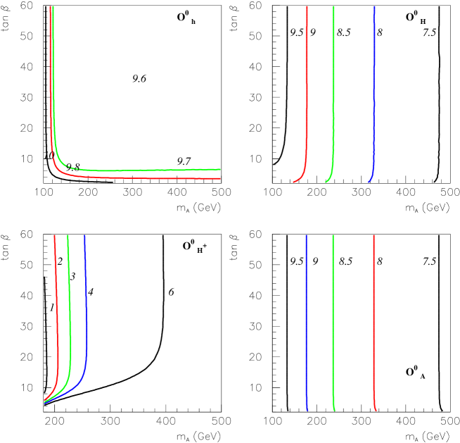
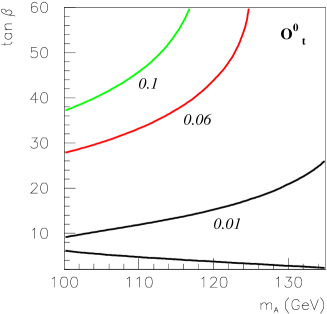
Figure 1: $O^{o}$ contour lines in the ($m_{A^{o}},\tan\beta$) plane predicted within the MSSM. The input parameters are defined in the text.

We next analyze the theoretical uncertainties in the evaluation of the ratios in eq.(LABEL:eq.interobsH) and eq.(2) coming from the experimental errors in the values of the SM parameters involved in their determination, at one-loop and order $\alpha_{S}$. We have found that the only significant errors are the ones coming from errors in the bottom and top quark masses and in the strong coupling constant $\alpha_{S}$. We have used the results from [34]:

$$m^{\rm pole}_{b}=(4.6\pm 0.2)\,{\rm GeV},\quad m_{t}=(174.3\pm 5.1)\,{\rm GeV},\quad\alpha_{S}(M_{Z}^{2})=0.118\pm 0.002$$

The uncertainty coming from these experimental errors is $\delta O=\frac{O^{\prime}-O}{O}$, where $O$ is the observable evaluated taking central values for $m_{b}$, $m_{t}$, and $\alpha_{S}$, and $O^{\prime}$ is the observable evaluated with one parameter reaching one extreme value. In Table 2 the different uncertainties are summarized for three different values of $m_{A^{o}}$, in the region $\tan\beta=10-60$. We use $\delta O_{n}\equiv\delta O_{h^{o}},\ \delta O_{H^{o}},\ \delta O_{A^{o}}$, and $\delta O_{c}\equiv\delta O_{t}$ for $m_{A^{o}}=100$ GeV, while $\delta O_{c}\equiv\delta O_{H^{+}}$ for $m_{A^{o}}=250$ and $500$ GeV.

Notice that the corrections are approximately constant as a function of $\tan\beta$. The uncertainty related to the error in $m_{b}$ is the dominant one, and of the same size for all the observables. Finally, the uncertainty related to $m_{t}$ is significant for the charged Higgs boson and top quark cases, only in the vicinity of the corresponding kinematical thresholds. The total uncertainty in the sixth column has been evaluated as the sum in quadrature of the numbers in the previous three columns and the error coming from neglecting the ${\mathcal{O}}(\alpha^{2}_{S})$ corrections.

$\delta$	$m_{A^{o}}$	$\alpha_{s}$	$m_{b}$	$m_{t}$	Total
	100 GeV	$2\%$	$11\%$	$<1\%$	$12\%$
$\delta O_{n}$	250 GeV	$3\%$	$10\%$	$<1\%$	$12\%$
	500 GeV	$3\%$	$11\%$	$<1\%$	$12\%$
	100 GeV	$1\%$	$8\%$	$6\%$	$11\%$
$\delta O_{c}$	250 GeV	$1\%$	$10\%$	$7\%$	$13\%$
	500 GeV	$3\%$	$11\%$	$<1\%$	$12\%$

Table 2: Uncertainties in the ratios induced by the experimental errors in $m_{t}$, $m_{b}$, and $\alpha_{S}$ for three values of $m_{A^{o}}$, in the region $\tan\beta=10-60$. We use $\delta O_{n}\equiv\delta O_{h^{o}},\delta O_{H^{o}},\delta O_{A^{o}}$ and $\delta O_{c}\equiv\delta O_{t}$ for $m_{A^{o}}=100$ GeV, and $\delta O_{c}\equiv\delta O_{H^{+}}$ for $m_{A^{o}}=250,500$ GeV. The total uncertainty has been evaluated in quadrature and includes the error coming from neglecting the ${\mathcal{O}}(\alpha^{2}_{S})$ corrections.

In summary, the MSSM predictions for the previous Higgs boson observables are known up to an uncertainty of the order of 13%. Any extra correction must be larger than that to be visible.

3.4 Comparing a type II two higgs doublet model and the minimal supersymmetric standard model

Here we investigate the similarities and differences of the set of observables defined in Section 3.1, in a general 2HDMII as compared to the MSSM. For a given Higgs sector mass pattern that is compatible with the MSSM, the values of the observables at the tree level, and after including the standard QCD corrections, coincide with the corresponding ones in the MSSM. Note that the mixing angle in the neutral sector, $\alpha$, is a derived quantity in the MSSM, whereas in the 2HDMII it is an independent parameter (in principle $-\pi/2\leq\alpha\leq\pi/2$, but actually the range in $\alpha$ is further restricted if the Higgs potential is required to be bounded from below) and, hence, its value can be different in the two models. However, since the branching ratios in the numerator and denominator of our observables $O$ have the same dependence on $\alpha$, at the tree level the $O^{\rm tree}$ themselves are $\alpha$ independent (see eq.(LABEL:eq.treeobserv)). When the standard QCD corrections are included, this $\alpha$ independence is still maintained. On the other hand, the standard electroweak corrections from $W^{\pm}$, $Z$, $\gamma$ are also similar in both models and, as already said, they have been estimated to be below $1\%$ and can be ignored here. Therefore, the only differences, apart from the SUSY corrections, could come from the Higgs sector radiative corrections. As mentioned before, these are negligible in the MSSM but, in principle, could be larger in the 2HDMII. The reason is that these corrections involve the Higgs boson self-couplings which in the 2HDMII are not restricted by SUSY and, in principle, can be large. We have estimated these potentially different contributions from the Higgs sector to the one-loop level and for a Higgs boson mass pattern compatible with the MSSM, and they turn out to be very small, certainly well below the common ones discussed in the previous section.

In order to illustrate this we discuss the case of $A^{o}$. We show in Fig.2 the maximum absolute value of the difference between the MSSM and 2HDMII Higgs sector corrections for $O^{o}_{A^{o}}$ (after scanning the allowed range in $\alpha$), relative to the tree-level prediction $O^{\rm tree}_{A^{o}}$. More specifically, these differences come exclusively from the $\alpha$-dependent one-loop diagrams, and from the triangular one-loop diagrams involving the Higgs boson self-couplings. The contour lines separate the regions in the ($m_{A^{o}},\tan\beta$) plane where the maximum difference between the MSSM and 2HDMII is larger than 0.1%, between 0.05% and 0.1%, between 0.01% and 0.05%, and below 0.01%. In the region of interest, $m_{A^{o}}>84.1$ GeV [34], this difference is always less than 0.1%.

In summary, as announced, the basic difference between the MSSM and a general 2HDMII model, with respect to our observables, is that the large SUSY particle loop corrections do not exist in the second case. In the next section we discuss these contributions.

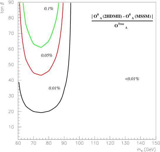
Figure 2: The maximum absolute value of the difference between the MSSM and 2HDMII Higgs sector corrections for $O^{o}_{A^{o}}$ (after scanning the allowed range in $\alpha$), relative to the tree-level prediction, $O^{\rm tree}_{A^{o}}$. Note that the area $m_{A^{o}}<84.1$ GeV (if $\tan\beta>1$) is already experimentally excluded at $95\%$ CL [34].

4 Results and discussion

In this section we present the numerical results for the SUSY QCD corrections to the set of observables $O_{h^{o}}$, $O_{H^{o}}$, $O_{A^{o}}$, $O_{H^{+}}$, and $O_{t}$. The relevant parameters in this discussion are $\tan\beta$, $m_{A^{o}}$, $\mu$, and $M_{\rm SUSY}$ ($M_{\rm SUSY}\sim M_{\tilde{q}}\sim M_{\tilde{g}}$). We first discuss the behavior with $\tan\beta$. In order to focus on this $\tan\beta$ dependence, we consider the simplest choice for the SUSY mass parameters, that is, $M_{\rm SUSY}=M_{\tilde{g}}=|\mu|$. We show in Figs. 3-5 the results for three $m_{A^{o}}$ values in the large, medium, and low $m_{A^{o}}$ regions: $m_{A^{o}}=500$, $250$, and $100\,{\rm GeV}$, respectively. The central lines in these figures follow the predictions for the observables without the SUSY QCD contribution, namely, $O^{o}$. The corresponding total theoretical uncertainties, discussed in Section 3.2, are shown as shaded bands around the central values. The bold lines represent the SUSY QCD corrected predictions for $\mu>0$ (solid) and $\mu<0$ (dashed). The observable $O_{t}$ appears in the lower left plot of Fig. 5 replacing $O_{H^{+}}$, since in this case $m_{t}>m_{H^{+}}+m_{b}$.

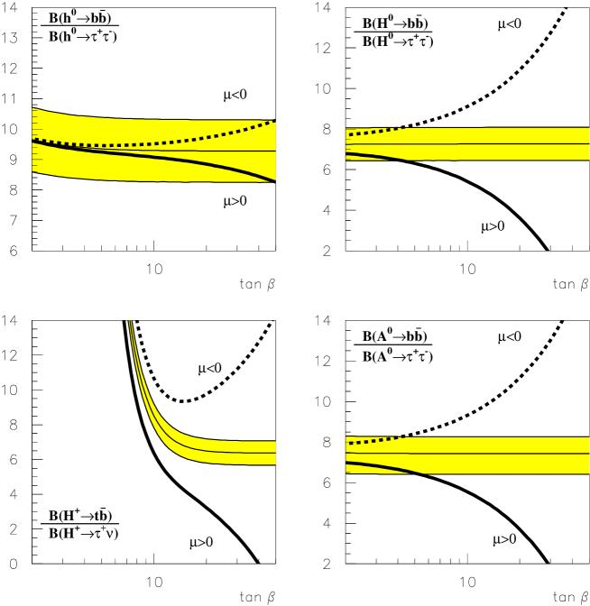
Figure 3: Predictions for $O_{h^{o}}$, $O_{H^{o}}$, $O_{H^{+}}$, and $O_{A^{o}}$ as a function of $\tan\beta$, for $m_{A^{o}}=500$ GeV. The central lines are the corresponding predictions for $O^{o}$. The shaded bands cover the theoretical uncertainties estimated in Sect. 3.3. The bold lines represent the SUSY QCD corrected predictions for $M_{\rm SUSY}=M_{\tilde{g}}=|\mu|$.

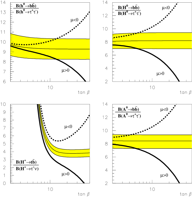
Figure 4: Same as in Fig. 3, but for $m_{A^{o}}=250$ GeV.

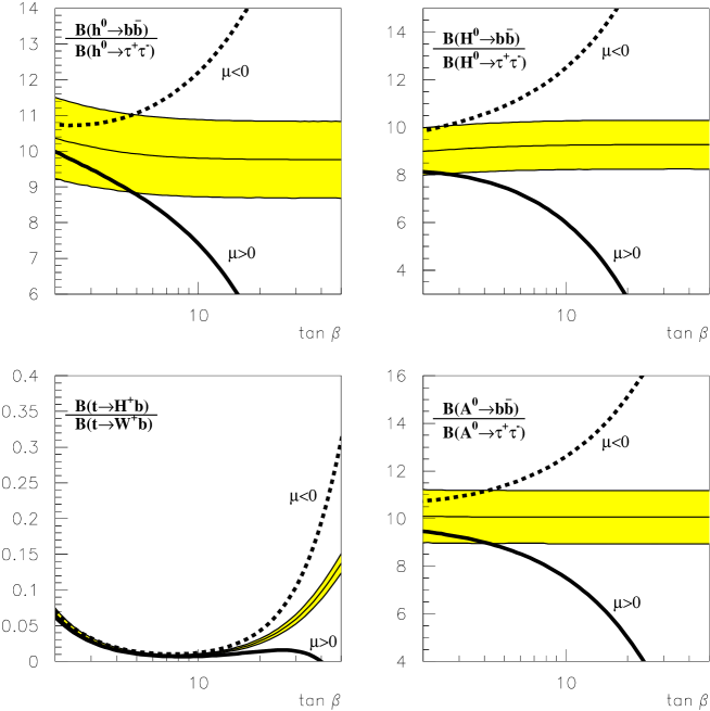
Figure 5: Same as in Fig. 3, but for $m_{A^{o}}=100$ GeV. The prediction for $O_{t}$ appears in the lower left plot instead of $O_{H^{+}}$, since in this case $m_{t}>m_{H^{+}}+m_{b}$.

One can see from the figures that, first, the predictions for all the observables separate from the central values as $\tan\beta$ grows. The sign of the SUSY QCD corrections is positive for $\mu<0$ and negative for $\mu>0$. The central values and their theoretical uncertainties are rather insensitive to $\tan\beta$ in the $H^{o}$ and $A^{o}$ channels. For the $h^{o}$, there is a very slight dependence at low $\tan\beta$, while for the $H^{+}$ this dependence is very strong in the low $\tan\beta$ region and it softens for $\tan\beta>15$, as expected from eq. (3). In any case, the predictions for all the Higgs boson observables without the SUSY QCD contributions are $\tan\beta$ insensitive in the large $\tan\beta$ region. This is very different for the top quark observable: it depends strongly on $\tan\beta$ in all the parameter space.

Concerning the size of the SUSY QCD corrections, we see that there is always a $\tan\beta$ region where these are larger than the theoretical uncertainties. For $m_{A^{o}}=500$ GeV and $m_{A^{o}}=250$ GeV, the observables $O_{A^{o}}$ and $O_{H^{o}}$ behave similarly and the predictions are outside the shaded band for $\tan\beta>5$. For $m_{A^{o}}=100$ GeV, the crossing still happens at $\tan\beta>5$ for $A^{o}$, whereas for $H^{o}$ the bold lines lie outside the error band in the whole region $2<\tan\beta<50$.

In the $h^{o}$ case the situation is qualitatively different. For $m_{A^{o}}=500$ GeV, the SUSY QCD correction is below the theoretical uncertainty for all values in the region $2<\tan\beta<50$. This is a manifestation of the decoupling of this correction for large $m_{A^{o}}$ values, as commented in Section 3.1. For smaller values of $m_{A^{o}}$, such as $m_{A^{o}}=250,100$ GeV, the decoupling has not effectively operated yet and the SUSY QCD corrections are sizable for large enough $\tan\beta$. In particular, for $m_{A^{o}}=250\ (100)$ GeV, they are larger than the theoretical error band for $\tan\beta>15\ (5$).

Regarding the charged Higgs boson case, two different situations must be considered. For $m_{A^{o}}=100$ GeV, where the decay into a top and a bottom quark is not kinematically allowed, the observable $O_{t}$ is considered. Otherwise, for $m_{A^{o}}=250$ GeV and $m_{A^{o}}=500$ GeV, the relevant observable is $O_{H^{+}}$. As can be seen in Fig. 5, the SUSY QCD corrections in $O_{t}$ for $m_{A^{o}}=100$ GeV are above the theoretical uncertainty for $\tan\beta>15$. However, as pointed out in Sect. 2, the central value prediction also depends strongly on $\tan\beta$ (and $m_{A^{o}}$) and it will be difficult to identify the effect of the SUSY QCD corrections above the additional uncertainty related to the experimental errors on the measurement of $\tan\beta$ and $m_{A^{o}}$. For $O_{H^{+}}$ and $m_{A^{o}}=500,250$ GeV both requirements, the correction being larger than the theoretical error and the leading contribution being insensitive to $\tan\beta$, are satisfied for values larger than about 15.

We next discuss the $M_{\rm SUSY}$ dependence. For this purpose, we fix the $|\mu|$ value to 250 GeV and choose $M_{\tilde{g}}=M_{\rm SUSY}$. Figure 6 shows the predictions for the observables as a function of $M_{\rm SUSY}$ for $m_{A^{o}}=250$ GeV, $\tan\beta=30$, and both signs of the $\mu$ parameter. Since, in this case, the SUSY QCD corrections vary as $1/M_{\rm SUSY}$, their size will be below the theoretical uncertainty for large enough $M_{\rm SUSY}$. This occurs in Fig. 6 for $O_{H^{o}}$, $O_{A^{o}}$, $O_{H^{+}}$, and $O_{t}$ at about 1500 GeV. For $O_{h^{o}}$ it is at about 500 GeV. Therefore, except in the light Higgs boson case, we expect the observables to be sensitive to indirect signals of supersymmetry via these SUSY QCD corrections up to quite large values of $M_{\rm SUSY}$.

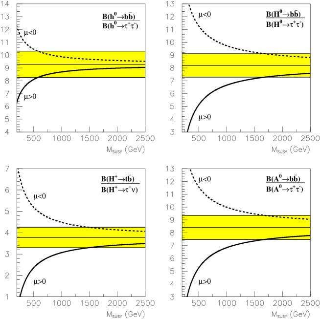
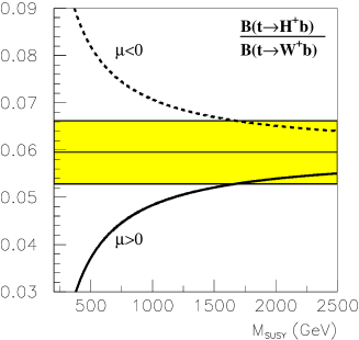
Figure 6: Predictions for $O_{h^{o}}$, $O_{H^{o}}$, $O_{H^{+}}$, $O_{A^{o}}$, and $O_{t}$ as a function of $M_{\rm SUSY}=M_{\tilde{g}}$, for $|\mu|=250$ GeV and $\tan\beta=30$. $m_{A^{o}}$ is fixed to 250 GeV for the observables $O_{h^{o}}$, $O_{H^{o}}$, $O_{H^{+}}$, and $O_{A^{o}}$. For $O_{t}$, $m_{A^{o}}=100$ GeV.

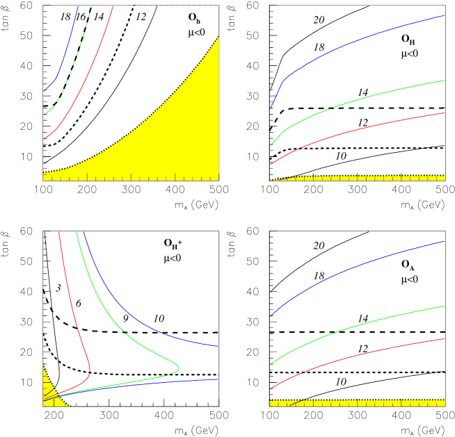
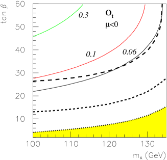
Figure 7: Predictions for the observables including the SUSY QCD corrections for $M_{\rm SUSY}=M_{\tilde{g}}=|\mu|$ and $\mu<0$. The solid contour lines follow the points in the $(m_{A^{o}},\tan\beta)$ plane with constant value of $O$. The shaded area represents the region where the corrections are smaller than the theoretical uncertainty. The long (short) dashed lines join the points where an experimental resolution of 50% (20%) is required to achieve a meaningful measurement.

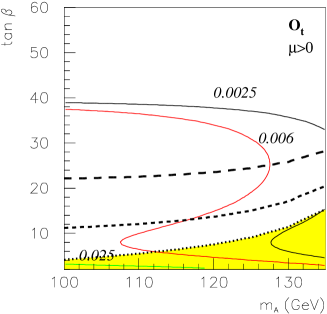
Figure 8: Same as in Fig.7, but for $\mu>0$.

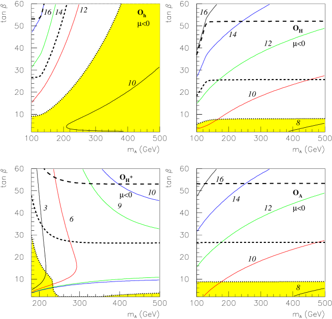
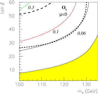
Figure 9: Predictions for the observables with the SUSY QCD corrections reduced by $50\%$ in order to simulate the effect of the SUSY EW contributions in the conservative scenario discussed in the text. The rest of the inputs and specifications are as in Fig. 7.

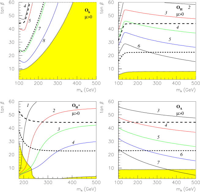
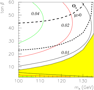
Figure 10: Same as in Fig.9, but for $\mu>0$.

We finally turn to the question of the experimental resolution required to evidence the above effects, after a Higgs boson signal is found at a given position in the $(m_{A^{o}},\tan\beta)$ parameter plane. The predictions for the observables including the SUSY QCD corrections for $M_{\rm SUSY}=M_{\tilde{g}}=|\mu|$ are shown in Fig. 7 for $\mu<0$ and in Fig. 8 for $\mu>0$. Comparing these figures with Fig. 1, the patterns of the $O$ (solid) contour lines change noticeably with respect to the ones for $O^{o}$. The differences are mainly because of both the large size of the corrections and the different behavior with $\tan\beta$.

The shaded zone in each plot represents the region where the corrections (if existing) are totally hidden inside the theoretical uncertainty discussed in Sect 3.3. Even the perfect experiment with infinite statistics and perfect resolution cannot make conclusions about the size of the corrections. This zone is particularly large for the SM-like $h^{o}$ covering a large fraction of the LHC “hole” (see Sect. 2). On the other hand, to have a decoupling channel can be useful as it can provide the “calibration” of what should be expected for the other channels without corrections.

In all plots in Figs. 7 and 8, the space above the long dashed line is the plane region that could be accessed experimentally with a modest resolution of 50% in $O$. Except for the $h^{o}$, nearly all points with $\tan\beta\gtrsim 20-25$ are testable at the one sigma level. The zone above the short dashed line requires an experimental resolution of 20%. Again with the exception of $h^{o}$, this zone covers approximately the region $\tan\beta\gtrsim 10-15$. Therefore, if an experimental resolution of $20\%$ can be achieved at the Tevatron and LHC, the analysis of the observables proposed in Sect. 3 could be used to search for indirect signals of SUSY in the main part of the relevant regions 1 and 2 discussed in Sect. 2.

Finally, we estimate the effect of the extra non-decoupling corrections from the SUSY EW sector. As discussed in Sect. 3.2, for very large $A_{t}$ values, the SUSY EW corrections do not decouple and this could increase or decrease the nondecoupling effect of the SUSY QCD corrections. For the present assumption of equally large SUSY parameters and by choosing a particular combination of signs that maximizes the size of $\Delta m_{b}^{SEW}$, we find that this contribution always remains below $50\%$ of the $\Delta m_{b}^{SQCD}$ one. In order to be conservative, we have performed the exercise of considering this pessimistic case where the SUSY EW corrections reduce the SUSY QCD signal by $50\%$ (see Figs. 9 and 10). As in Figs. 7 and 8, the shaded zone in each plot represents the region where the corrections are completely hidden inside the theoretical uncertainty. The long (short) dashed lines again limit the zones where an experimental resolution of $50\%$ ($20\%$) is required to achieve a meaningful measurement.

Figures 9 and 10 show that, as expected, the reachable values of $\tan\beta$ would approximately double the ones in Figs. 7 and 8. Also, the shaded area has doubled. The points with $\tan\beta\gtrsim 45-55$ are testable at the one sigma level with a resolution of $50\%$; $\tan\beta\gtrsim 20-25$ with a resolution of $20\%$. In summary, even in this pessimistic case providing SUSY EW corrections of considerable size, a large region in the $(m_{A},\tan\beta)$ plane remains testable.

5 Conclusions

In this paper we have looked for indirect signals of a heavy supersymmetric spectrum via its contributions to the radiative corrections to Higgs boson decays. For that purpose we have analyzed the dominant SUSY QCD corrections, coming from heavy squarks and gluinos, to the Higgs boson decays into quarks. We have studied in detail the nondecoupling contributions, especially in the large $\tan\beta$ region where their size is large. In order to search for these SUSY signals, we have proposed a set of observables consisting of ratios of Higgs branching ratios into third-generation quarks ($H^{o},h^{o},A^{o}\to b\bar{b}$ and $H^{+}\to t\bar{b}$) divided by the corresponding ones into third-generation leptons ($H^{o},h^{o},A^{o}\to\tau^{+}\tau^{-}$ and $H^{+}\to\nu\tau^{+}$). In addition, the observable for top quark decays given by the ratio of $B(t\to H^{+}b)$ divided by $B(t\to W^{+}b)$, complementary to the previous charged Higgs boson observable in the low $m_{A^{o}}$ region, has been analyzed. These observables are optimal for this purpose since the SUSY QCD corrections appear just in the decays to quarks and, therefore, the decays into leptons can be used as control channels.

We have carefully studied any sources of uncertainty that would modify the prediction of the observables, previous to the SUSY QCD corrections. In particular, the theoretical uncertainties coming from the QCD corrections, and from the errors in the values of the SM parameters involved in the determination of these observables, have been evaluated. In addition, it has been found that the SUSY QCD corrections will allow one to discriminate between the MSSM and a nonsupersymmetric 2HDMII, even in the case of a similar Higgs sector mass pattern.

Our detailed study of this set of observables has revealed their high sensitivity to the SUSY QCD contributions and shown that they are sizable in most of the ($m_{A^{o}},\tan\beta$) plane. The corrections to the different observables are strongly correlated. A global analysis of all of them, together with the experimental determination of $m_{A^{o}}$ and $\tan\beta$, will be part of the search for supersymmetric signals at future colliders, especially if the SUSY spectrum turns out to be very heavy. The measurement of these observables should be the next step after a Higgs boson discovery at the LHC or the Tevatron. We have seen that, with a modest experimental resolution of 50%, the observables would show evidence of the SUSY QCD corrections to the $A^{o}$, $H^{o}$, and $H^{+}$ decay widths, if $\tan\beta\gtrsim 20-25$. A better resolution of $20\%$ would show the corrections down to $\tan\beta\gtrsim 10-15$. Our study of the SUSY EW effects shows that, even in the pessimistic case where the SUSY QCD corrections get reduced by $50\%$, an experimental resolution of $20\%$ would expose the SUSY corrections down to $\tan\beta\gtrsim 20-25$. Observation of the corrections in the $h^{o}$ case would require, in general, quite large values of $\tan\beta$. We hope our study will encourage our colleagues of CDF, D0, ATLAS, and CMS to investigate the actual performance of their detectors.

References

- [1] J. F. Gunion, H. E. Haber, Nucl. Phys. B272, 1 (1986); B278, 449 (1986) [E: B402, 567 (1993)]; J. F. Gunion, H. E. Haber, G. Kane, and S. Dawson, The Higgs Hunter’s Guide (Addison-Wesley, Reading, MA, 1990); J. F. Gunion and H. E. Haber, hep-ph/9302272.
- [2] H.E. Haber, and G.L. Kane, Phys. Rep. 117, 75 (1985).
- [3] H. E. Haber and R. Hempfling, Phys. Rev. Lett. 66, 1815 (1991); Phys. Rev. D48, 4280 (1993); Y. Okada, M. Yamaguchi and T. Yanagida, Prog. Theor. Phys. 85, 1 (1991); Phys. Lett. B262, 54 (1991); J. Ellis, G. Ridolfi and F. Zwirner, Phys. Lett. B257, 83 (1991); Phys. Lett. B262, 477 (1991); R. Barbieri and M. Frigeni, Phys. Lett. B258, 167 (1991); Phys. Lett. B258, 395 (1991). For an updated study see: M. Carena, H. E. Haber, S. Heinemeyer, W. Hollik, C. E. M. Wagner and G. Weiglein, Nucl. Phys. B580, 29 (2000); J. R. Espinosa and R.-J. Zhang, J. High Energy Phys. 0003, 026 (2000); Nucl. Phys. B586, 3 (2000), and references therein.
- [4] D. M. Pierce, J. A. Bagger, K. Matchev and R.-J. Zhang, Nucl. Phys. B491, 3 (1997).
- [5] M. Carena et al., “Report of the Tevatron Higgs Working Group of the Tevatron Run 2 SUSY/Higgs Workshop”, hep-ph/0010338.
- [6] ATLAS Technical Design Report, CERN-LHCC-99-15, (1999); CMS Technical Proposal, CERN-LHCC-94-43, (1994).
- [7] H. E. Haber and Y. Nir, Nucl. Phys. B335, 363 (1990); H. E. Haber, in Proceedings of the US–Polish Workshop, Warsaw, Poland, 1994, edited by P. Nath, T. Taylor, and S. Pokorski (World Scientific, Singapore, 1995) pp. 49–63.
- [8] M. Spira, Fortsch. Phys. 46, 203 (1998).
- [9] A. Dabelstein, Nucl. Phys. B456, 25 (1995).
- [10] J. A. Coarasa, R. A. Jiménez and J. Solà, Phys. Lett. B389, 312 (1996).
- [11] R. A. Jiménez and J. Solà, Phys. Lett. B 389, 53 (1996).
- [12] A. Bartl, H. Eberl, K. Hidaka, T. Kon, W. Majerotto and Y. Yamada, Phys. Lett. B 378, 167 (1996).
- [13] J. A. Coarasa, D. Garcia, J. Guasch, R. A. Jiménez and J. Solà, Phys. Lett. B 425, 329 (1998).
- [14] J. Guasch, R. A. Jiménez and J. Solà, Phys. Lett. B 360, 47 (1995).
- [15] J. A. Coarasa, D. Garcia, J. Guasch, R. A. Jiménez and J. Solà, Eur. Phys. J C2, 373 (1998).
- [16] M. Carena, S. Mrenna and C. E. M. Wagner, Phys. Rev. D60, 075010 (1999); Phys. Rev. D62, 055008 (2000).
- [17] F. Borzumati, G. R. Farrar, N. Polonsky and S. Thomas, Nucl. Phys. B555, 53 (1999).
- [18] K.S. Babu and C. Kolda, Phys. Lett. B451, 77 (1999).
- [19] M. Carena, D. Garcia, U. Nierste and C. E. Wagner, Nucl. Phys. B 577, 88 (2000).
- [20] H. Eberl, K. Hidaka, S. Kraml, W. Majerotto and Y. Yamada, Phys. Rev. D 62,055006 (2000).
- [21] H. E. Haber, M. J. Herrero, H. E. Logan, S. Peñaranda, S. Rigolin and D. Temes, Phys. Rev. D 63, 055004 (2001).
- [22] M. J. Herrero, S. Peñaranda, and D. Temes, Phys. Rev. D 64, 115003 (2001).
- [23] A. Dobado, M. J. Herrero and D. Temes, Phys. Rev. D (to be published), hep-ph/0107147.
- [24] A. Dobado, M. J. Herrero and S. Peñaranda, Eur. Phys. J. C 7 313 (1999); In Barcelona 1997, Quantum effects in the minimal supersymmetric standard model edited by J. Solà (World Scientific Singapore,1998), pp. 266-286; A. Dobado, M. J. Herrero and S. Peñaranda, hep-ph/9711441; Eur. Phys. J. C 12 673 (2000); 17, 487 (2000).
- [25] M. Carena, H. E. Haber, H. E. Logan, S. Mrenna, Phys Rev. D (to be published), hep-ph/0106116.
- [26] M.J. Herrero, invited talk at the XXIX International Meeting on Fundamental Physics, Sitges, Barcelona, Spain, 2001 (to be published). Report No. FTUAM/ 01-11. Slides available at .
- [27] CDF Collaboration, F. Abe et al. Phys. Rev. Lett. 81, 5748 (1998); CDF Collaboration, T. Affolder et al. ibid 86, 4472 (2001).
- [28] CDF Collaboration, F. Abe et al. Phys. Rev. Lett. 78, 2906 (1997); M. Drees, M. Guchait, and P. Roy, ibid 80, 2047 (1998); ibid 81, 2394 (1998).
- [29] CDF Collaboration, T. Affolder et al. Phys. Rev. D62, 012004 (2000); CDF Collaboration, F. Abe et al., Phys. Rev. Lett. 79, 357 (1997); D0 Collaboration, B. Abbott et al., Phys. Rev. Lett. 82, 4975 (1999).
- [30] H. E. Haber, M. J. Herrero, H. E. Logan, S. Peñaranda, S. Rigolin and D. Temes, hep-ph/0102169. M. J. Herrero, invited talk at the RADCOR-2000 Symposium, Carmel, CA, 2000 (to be published). Slides available at: .
- [31] J. Guasch, W. Hollik and S. Peñaranda, Phys. Lett. B515, 367 (2001).
- [32] A. Djouadi, J. Kalinowski, and M. Spira, Comput. Phys. Commun. 108, 56 (1998).
- [33] M. Carena, J.R. Espinosa, M. Quiros, and C.E.M. Wagner, Phys. Lett. B355, 209 (1995); M. Carena, M. Quiros, and C.E.M. Wagner, Nucl. Phys. B461, 407 (1996).
- [34] Particle Data Group, D. E. Groom et al., Eur. Phys. J. C15, 1 (2000).