Event-by-event fluctuations in hydrodynamical description of heavy-ion collisions

Abstract

Effects caused by the event-by-event fluctuation of the initial conditions in hydrodynamical description of high-energy heavy-ion collisions are investigated. Non-negligible effects appear for several observable quantities, even for a fixed impact parameter $\vec{b}\,$. They are sensitive to the equation of state, being the dispersions of the observable quantities in general smaller when the QGP phase appears at the beginning of hydrodynamic evolution than when the fluid remains hadron gas during whole the evolution.

1 INTRODUCTION

In usual hydrodynamic description of high-energy heavy-ion collisions, one customarily assumes some highly symmetric and smooth initial conditions, which correspond to mean distributions of velocity, temperature, energy density, etc., averaged over several events. However, our systems are not large enough, so large fluctuations are expected. What are the effects of the event-by-event fluctuation of the initial conditions? Are they sizable? Do they depend on the equation of state? Which are the most sensitive variables? These are some questions which arise regarding such an initial-state fluctuation, and we try to shed some light on these matters in the present study[1].

2 METHOD OF STUDY

In order to study the problem stated above, first we generate events by using the NeXus event generator[2], from which initial conditions are computed at the time $\tau=1~{}$fm. Then, the hydrodynamic equations are solved, starting from these initial conditions, assuming some equation of state (EoS). To see the EoS dependence of the effects we are treating, we consider two different EoS’s[3]:

1. Resonance Gas (RG): $c_{s}\,^{2}=0.2\,$;

2. $$\mbox{QGP+RG:}\ c_{s}\,^{2}=\left\{\begin{array}[]{ll}0.2\,,&\varepsilon<0.28\,\mbox{GeV/fm}^{3},\\ 0.056/\varepsilon,&\mbox{mixed phase}\,,\\ 1/3-4B/3\varepsilon,&\varepsilon>1.45\,\mbox{GeV/fm}^{3}.\end{array}\right.$$

The resolution of the hydrodynamic equations deserves some special care, since our initial conditions do not have any symmetry nor they are smooth. We adopt the so-called smoothed-particle hydrodynamic (SPH) approach[4], first used in astrophysics and which we have previously adapted for heavy-ion collisions[5], a method flexible enough, giving a desired precision. The main characteristic of SPH is the parametrization of the flow in terms of discrete Lagrangian coordinates attached to small volumes (called “particles”) with some conserved quantity. In the present work, besides the energy and momentum, we took the entropy as our conserved quantity. Then, its density (in the space-fixed frame) is parametrized as

$$s^{*}({\bf x},t)=\sum_{i}^{N}\nu_{i}~{}W({\bf x}-{\bf x}_{\,i}(t);h)~{},$$ (1)

where

$$\left\{\begin{array}[]{l}W({\bf x}-{\bf x}_{\,i}(t);h)\mbox{ is a normalized kernel};\\ {\bf x}_{\,i}(t)\mbox{ is the }i\mbox{-th particle position, so the velocity is }{\bf v}_{\,i}=d{\bf x}_{\,i}/dt\ ;\\ h~{}\mbox{is the smoothing scale parameter;}\end{array}\right.$$

and we have

$$S=\int\!d^{3}{\bf x}~{}s^{*}({\bf x},t)=\sum_{i}^{N}\nu_{i}~{}.$$ (2)

The equations of motion are then written as the coupled equations

$$\frac{d}{dt}\left(\nu_{i}\frac{P_{i}+\varepsilon_{i}}{s_{i}}\gamma_{i}{\bf v}_{i}\right)+\sum_{j}\nu_{j}\bigg{[}\frac{P_{i}}{{s^{*}_{i}}^{2}}+\frac{P_{j}}{{s^{*}_{j}}^{2}}\bigg{]}\,{\bf\nabla}_{i}W({\bf x}_{\,i}-{\bf x}_{\,j};h)=0\,.\ \ \$$ (3)

Following this procedure, we computed some observable quantities, event-by-event, for $\sqrt{s}=$130$A$GeV $Au+Au$ collisions. The results are presented in the next Section.

3 RESULTS

3.1 Elliptic flow coefficient $v_{2}$

Having solved the coupled equations (3), we have computed the particle spectra at $T=m_{\pi}\,$ and from which the elliptic flow coefficient $v_{2}\,$ on an event-by-event basis. In Figure 1, we show its distributions for a fixed impact parameter $b$, for the two EoS considered. As expected, $v_{2}$ exhibits a large fluctuation, which depends on the EoS. One should take care in looking at this Figure that our $b$ is the true impact parameter (not determined in the way experimentalists do), so for instance in the RG case, there are some events with negative $v_{2}\,$, which experimentally would not appear. As for the average values $<\!v_{2}\!>\,$, it is almost independent of the EoS. This is shown in Figure 2, where $<v_{2}>\pm\,\delta v_{2}$ is plotted as function of the centrality and compared with data[6]. It is seen that $<\!v_{2}\!>$ reproduces well the experimental trend, whereas the dispersions $\delta v_{2}$ are much wider than the experimental errors. As for the EoS dependence, $\delta v_{2}$ is smaller when QGP is produced.

Figure 1: Distribution of elliptic-flow coefficients $v_{2}$ at $b=10~{}$fm for two EoS.

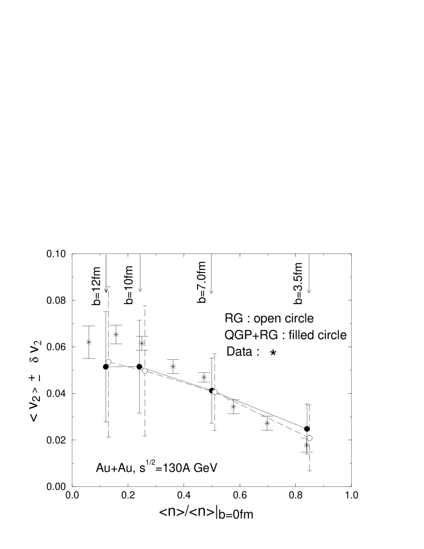
Figure 2: EoS dependence of $<v_{2}>\pm\,\delta v_{2}$ as function of the centrality, compared with data[6].

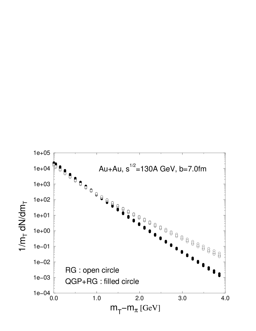
Figure 3: Pion $m_{T}$ spectra for 5 events ($b=7.0~{}$fm).

3.2 $m_{T}$ distributions

In Figure 3, we show the $m_{T}$ distributions for 5 events. As expected, $m_{T}$ distributions are in general steeper when QGP is produced. As for fluctuations, the resultant fluctuation in $m_{T}$ spectrum (or in the slope parameter $\delta\tilde{T}$) is very small.

3.3 Multiplicity fluctuation in the mid-rapidity region

Table 1 summarizes the results of our study on multiplicity fluctuation in the mid-rapidity region. It is seen that i) as $b\rightarrow 0$, $<n_{\pi}>$ becomes much larger with the QGP EoS; ii) $\delta n_{\pi}$ shows the same tendency in this limit; iii) As for the ratio $\delta n_{\pi}/\!<n_{\pi}>$, it is not sensitive to the EoS.

Table 1: EoS dependence of the multiplicity fluctuation in two different rapidity intervals $-\Delta y<y<+\Delta y$, as function of the impact parameter $b$.

$b~{}$[fm]	EoS	# of	$\Delta y$=1.875			$\Delta y$=3.00
		events	$\!<\!\!n\!\!>\$	$\delta n$	$\delta n/\!\!<\!\!n\!\!>$	$\!<\!\!n\!\!>\$	$\delta n\ \$	$\delta n/\!\!<\!\!n\!\!>$
3.5	RG	44	1029.7	46.2	0.045	1623.2	68.7	0.042
	QGP	38	1553.0	80.9	0.052	2544.6	129.0	0.051
7.0	RG	55	613.3	49.5	0.081	977.4	71.6	0.073
	QGP	58	926.1	81.1	0.087	1530.5	123.7	0.081
10.0	RG	166	312.8	43.0	0.137	506.1	65.8	0.130
	QGP	180	437.5	66.5	0.151	740.7	103.9	0.140
12.0	RG	79	162.8	35.6	0.219	268.9	56.2	0.209
	QGP	100	220.1	52.8	0.240	379.8	85.2	0.224

4 CONCLUSIONS AND OUTLOOK

The present study shows that the effects of the event-by-event fluctuation of the initial conditions in hydrodynamics are sizable and should be considered in data analyses. They do depend on the equation of state. Among the quantities examined here, $\delta v_{2}$ is the most sensitive to the equation of state.

In the present work, many important factors have not been considered: baryon-number conservation, strangeness production, resonance decays, continuous emission effects, spectators, etc., which should indeed taken into account in order to get more precise results. Especially, use of the same procedure for the determination of the centrality as used by experimentalists, as in[6], will make the results more directly comparable with data. In any event, we believe that the effects we studied will be present and will be sizable, even with these improvements.

References

- [1] The preliminary version appeared in T. Osada, C.E. Aguiar, Y. Hama and T. Kodama, Event-by-event analysis of ultra-relativistic heavy-ion collisions in smoothed particle hydrodynamics, arXiv: nucl-th/0102011.
- [2] H.J. Drescher, M. Hladik, S. Ostrapchenko, T. Pierog and K. Werner, J.Phys. G25 (1999) L91; Nucl.Phys. A661 (1999) 604.
- [3] C.M. Hung and E.V. Shuryak, Phys. Rev. Lett. 75 (1995) 4003.
- [4] L.B. Lucy, Ap. J. 82 (1977) 1013; R.A. Gingold and J.J. Monaghan, Mon.Not.R.Astr.Soc. 181 (1977) 375.
- [5] C.E. Aguiar, T. Kodama, T. Osada and Y. Hama, J.Phys. G27 (2001) 75, and references therein.
- [6] STAR Collaboration, K.H. Ackermann et al., Phys.Rev.Lett. 86 (2001) 402.