W08 NUCLEON FORM FACTORS IN THE SPACE- AND TIMELIKE REGIONS

Abstract

Dispersion relations provide a powerful tool to describe the electromagnetic form factors of the nucleon both in the spacelike and timelike regions with constraints from unitarity and perturbative QCD. We give a brief introduction into dispersion theory for nucleon form factors and present results from a recent form factor analysis. Particular emphasis is given to the form factors in the timelike region. Furthermore, some recent results for the spacelike form factors at low momentum transfer from a ChPT calculation by Kubis and Meißner are discussed.

1 INTRODUCTION

A detailed understanding of the electromagnetic form factors of the nucleon is important for revealing aspects of both perturbative and nonperturbative nucleon structure. The form factors also contain important information on nucleon radii and vector meson coupling constants. Moreover, the form factors are an important ingredient in a wide range of experiments such as Lamb shift measurements [1] and measurements of the strangeness content of the nucleon [2]. With the advent of the new continuous beam electron accelerators like CEBAF (Jefferson Lab.), MIT-Bates, and MAMI (Mainz), a wealth of precise data for spacelike momentum transfers has become available. Due to the difficulty of the experiments, the timelike form factors are less well known. While there is a fair amount of information on the proton timelike form factors, only one measurement of the neutron form factor from the pioneering FENICE experiment [3] exists.

The basic theoretical framework of dispersion theory for nucleon form factors was established long ago [4, 5]. In recent years, these methods have been refined considerably. In particular, constraints from perturbative QCD and independent low-energy experiments (e.g. on the neutron radius) have been incorporated [6, 7].

In the first part of this paper, we review the status of dispersion theory for nucleon form factors and show results from a recent update [6, 7]. In the second part, we discuss the effective field theory description of nucleon form factors in the framework of ChPT, based on a recent calculation by Kubis and Meißner[8].

2 FORMALISM

Using Lorentz and gauge invariance, the nucleon matrix element of the electromagnetic (em) current operator $j_{\mu}^{\rm em}$ can be parametrized in terms of two form factors,

$$\langle p^{\prime}|j_{\mu}^{\rm em}|p\rangle=\bar{u}(p^{\prime})\left[F_{1}(t)\gamma_{\mu}+i\frac{F_{2}(t)}{2M}\sigma_{\mu\nu}q^{\nu}\right]u(p)\,,$$ (1)

where $M$ is the nucleon mass and $t=(p^{\prime}-p)^{2}=q^{2}<0$ the four-momentum transfer. $F_{1}$ and $F_{2}$ are the Dirac and Pauli form factors, respectively. They are normalized at $t=0$ as

$$F_{1}^{p}(0)=1\,,\;F_{1}^{n}(0)=0\,,\;F_{2}^{p}(0)=\kappa_{p}\,,\;F_{2}^{n}(0)=\kappa_{n}\,,$$ (2)

with $\kappa_{p}=1.79$ and $\kappa_{n}=-1.91$ the anomalous magnetic moments of protons and neutrons in nuclear magnetons, respectively. It is convenient to work in the isospin basis and to decompose the form factors into isoscalar and isovector parts,

$$F_{i}^{s}=\frac{1}{2}(F_{i}^{p}+F_{i}^{n})\,,\quad F_{i}^{v}=\frac{1}{2}(F_{i}^{p}-F_{i}^{n})\,,$$ (3)

where $i=1,2\,$. The experimental data are usually given for the Sachs form factors

$$G_{E}(t) = F_{1}(t)-\tau F_{2}(t)\,,$$ (4)

$$G_{M}(t) = F_{1}(t)+F_{2}(t)\,,$$

where $\tau=-t/(4M^{2})$. In the Breit frame, $G_{E}$ and $G_{M}$ may be interpreted as the Fourier transforms of the charge and magnetization distributions, respectively.

3 NUCLEON FORM FACTORS IN DISPERSION THEORY

3.1 Spectral Decomposition

Based on unitarity and analyticity, dispersion relations relate the real and imaginary parts of the em nucleon form factors. Let $F(t)$ be a generic symbol for any one of the four nucleon form factors. We write down an unsubtracted dispersion relation of the form

$$F(t)=\frac{1}{\pi}\,\int_{t_{0}}^{\infty}\frac{{\rm Im}\,F(t^{\prime})}{t^{\prime}-t-i\epsilon}\,dt^{\prime}\,,$$ (5)

where $t_{0}$ is the threshold of the lowest cut of $F$. Since the normalization of $F$ is known, a once subtracted dispersion relation could be used as well. Eq. (5) relates the em structure of the nucleon to its absorptive behavior. The imaginary part entering Eq. (5) can be obtained from a spectral decomposition [4]. For this purpose it is convenient to consider the em current matrix element in the timelike region,

$$J_{\mu} = \langle N(p)\overline{N}(\bar{p})|j_{\mu}^{\rm em}(0)|0\rangle$$

$$= \bar{u}(p)\left[F_{1}(t)\gamma_{\mu}+i\frac{F_{2}(t)}{2M}\sigma_{\mu\nu}(p+\bar{p})^{\nu}\right]v(\bar{p})\,,$$

where $p\,,\bar{p}$ are the momenta of the nucleon-antinucleon pair created by the current $j_{\mu}^{\rm em}$. The four-momentum transfer in the timelike region is $t=(p+\bar{p})^{2}>0$. Using the LSZ formalism, the imaginary part of the form factors is obtained by inserting a complete set of intermediate states as [4]

$${\rm Im}\,J_{\mu} = \frac{\pi}{Z}(2\pi)^{3/2}{\cal N}\,\sum_{\lambda}\langle p|\bar{J}_{N}(0)|\lambda\rangle\qquad$$

$$\times\langle\lambda|j_{\mu}^{\rm em}(0)|0\rangle\,v(\bar{p})\,\delta^{4}(p+\bar{p}-p_{\lambda})\,,$$

where ${\cal N}$ is a nucleon spinor normalization factor, $Z$ is the nucleon wave function renormalization, and $\bar{J}_{N}(x)=J^{\dagger}(x)\gamma_{0}$ with $J_{N}(x)$ a nucleon source. The states $|\lambda\rangle$ are asymptotic states of momentum $p_{\lambda}$ which are stable with respect to the strong interaction. For the matrix elements in Eq. (3.1) to be nonvanishing, they must carry the same quantum numbers as as the current $j^{\rm em}_{\mu}$: $I^{G}(J^{PC})=0^{-}(1^{--})$ for the isoscalar component and $I^{G}(J^{PC})=1^{+}(1^{--})$ for the isovector component of $j^{\rm em}_{\mu}$. Furthermore, they have no net baryon number. For the isoscalar part the lowest mass states are: $3\pi$, $5\pi$, $\ldots$; for the isovector part they are: $2\pi$, $4\pi$, $\ldots$. Because of $G$-parity, states with an odd number of pions only contribute to the isoscalar part, while states with an even number contribute to the isovector part. Associated with each intermediate state is a cut starting at the corresponding threshold in $t$ and running to infinity. As a consequence, the spectral function ${\rm Im}\,F(t)$ is different from zero along the cut from $t_{0}$ to $\infty$ with $t_{0}=4\,(9)\,m_{\pi}^{2}$ for the isovector (isoscalar) case. Using Eqs. (3.1,3.1), the spectral functions for the form factors can in principle be constructed from experimental data. In practice, this proves a formidable task and is also unstable. However, the spectral function can be constrained using, for example, vector meson dominance.

3.2 Vector Meson Dominance

Within the vector meson dominance (VMD) approach, the spectral functions are approximated by a few vector meson poles, namely the $\rho,\ldots$ in the isovector and the $\omega,\phi,\ldots$ in the isoscalar channel, respectively. In that case, the form factors take the form

$$F_{i}^{I}(t)=\sum_{V_{I}}\frac{a_{i}^{V_{I}}}{m^{2}_{V_{I}}-t}\,\quad i=1,2\,;\,\quad I=v,s\,\,.$$ (8)

Clearly, such pole terms contribute to the spectral functions as $\delta$-functions,

$${\rm Im}\,F^{V_{I}}_{i}(t)=\pi\,a_{i}^{V_{I}}\,\delta(t-m_{V_{I}}^{2})\,\,.$$ (9)

These terms arise naturally as approximations to vector meson resonances in the continuum of intermediate states like $n\pi$ ($n\geq 2)$, $N\overline{N}$, $K\overline{K}$ and so on. If the continuum contributions are strongly peaked near the vector meson resonances, Eq. (8) is a good approximation.

For the contribution of the two-pion continuum to the isovector spectral functions, however, the replacement by a sharp $\rho$-resonance is not justified and strongly underestimates the isovector radius. The unitarity relation of Frazer and Fulco [10] determines the isovector spectral functions from $t=4\,m_{\pi}^{2}$ to $t\simeq 50\,m_{\pi}^{2}\simeq 1$ GeV² in terms of the pion form factor $F_{\pi}(t)$ and the P-wave $\pi\pi N\bar{N}$ partial wave amplitudes. The isovector spectral function is strongly enhanced close to the two-pion threshold (see, e.g., Fig. 2 in Ref. [6]). The reason for this behavior is well known. The corresponding partial waves have a branch point singularity on the second sheet (from the projection of the nucleon pole terms) located at $t_{c}=4m_{\pi}^{2}-m_{\pi}^{4}/M^{2}\approx 3.98\,m_{\pi}^{2}\,,$ very close to the physical threshold at $t_{0}=4m_{\pi}^{2}$. The isovector form factors inherit this singularity and the closeness to the physical threshold leads to the pronounced enhancement. Note that in the VMD approach this spectral function is given by a $\delta$-function peak at $m_{\rho}^{2}\simeq 30\,m_{\pi}^{2}$ and thus the isovector radii are strongly underestimated if one neglects the unitarity correction [11], as can be seen from the formula

$$\langle r^{2}\rangle_{i}^{v}=\frac{6}{\pi}\int_{4m_{\pi}^{2}}^{\infty}\frac{dt}{{t}^{2}}\,{\rm Im}\,F_{i}^{v}(t)\,\,.$$ (10)

In the isoscalar channel, it is believed that the pertinent spectral functions rise smoothly from the three-pion threshold to the $\omega$-peak, i.e. that there is no pronounced effect from the three-pion cut on the left wing of the $\omega$-resonance (which also has a much smaller width than the $\rho$). In chiral perturbation theory an investigation of the spectral functions to two loops has indeed shown no such enhancement [12], in contrast to the one loop calculation of the isovector nucleon form factors where the unitarity correction on the left wing of the $\rho$ has been seen. A form factor analysis in the described framework with three vector meson poles in both the isoscalar and isovector channels as well as the two-pion continuum was carried out by Höhler et al. [5]. In the following, we describe an extended update that also includes timelike data and additional contstraints on the spectral function.

3.3 Constraints

The first set of constraints concerns the low-$t$ behavior of the form factors. First, we enforce the correct normalization of the form factors, which is given in Eq. (2). Second, we constrain the neutron radius from a low-energy neutron-atom scattering experiment [13].

Perturbative QCD (pQCD) constrains the behavior of the nucleon em form factors for large momentum transfer. Brodsky and Lepage [14] find for $t\to-\infty$,

$$F_{i}(t)\to(-t)^{-(i+1)}\,\left[\ln\left(\frac{-t}{Q_{0}^{2}}\right)\right]^{-\gamma}\,,\quad i=1,2\,,$$ (11)

where $Q_{0}\simeq\Lambda_{\rm QCD}$. The anomalous dimension $\gamma$ depends weakly on the number of flavors, $\gamma=2.148$, $2.160$, $2.173$ for $N_{f}=3$, $4$, $5$, in order. The power behavior of the form factors at large $t$ can be easily understood from perturbative gluon exchange. In order to distribute the momentum transfer from the virtual photon to all three quarks in the nucleon, at least two massless gluons have to be exchanged. Since each of the gluons has a propagator $\sim 1/t$, the form factor has to fall off as $1/t^{2}$. In the case of $F_{2}$, there is additional suppression by $1/t$ since a quark spin has to be flipped.

In the form factor analysis, we used spectral functions that lead exactly to the large-$t$ behavior as given in Eq. (11). The spectral functions of the pertinent form factors are separated into a hadronic (meson pole) and a quark (pQCD) component as follows,

$$F_{i}^{s}(t)=\tilde{F}_{i}^{s}(t)L(t)$$ (12)

$$=\Bigg{[}\sum_{V_{s}}\frac{a_{i}^{V_{s}}\,L^{-1}(m^{2}_{V_{s}})}{m^{2}_{V_{s}}-t}\Bigg{]}\,\Bigg{[}\ln\Bigg{(}\frac{\Lambda^{2}-t}{Q_{0}^{2}}\Bigg{)}\Bigg{]}^{-\gamma}\,,$$

$$F_{i}^{v}(t)=\Bigg{[}\tilde{F}_{i}^{\rho}(t)+\sum_{V_{v}}\frac{a_{i}^{V_{v}}\,L^{-1}(m^{2}_{V_{v}})}{m^{2}_{V_{v}}-t}\Bigg{]}\,L(t)\,,$$

where $F_{i}^{\rho}(t)=\tilde{F}_{i}^{\rho}(t)\,L(t)^{-1}$ parametrizes the two-pion contribution (including the $\rho$) in terms of the pion form factor and the P-wave $\pi\pi\bar{N}N$ partial wave amplitudes in a parameter-free manner (for details see [6]). Furthermore, the parameter $\Lambda$ separates the hadronic from the quark contributions. The fits performed in [6, 7] are rather insensitive to the presence of the logarithmic factor in the spectral functions. The factor $L(t)$ in Eq. (12) contributes to the spectral functions for $t>\Lambda^{2}$ and in some sense parametrizes the intermediate states in the pQCD regime. The particular logarithmic form has been chosen for convenience. More important is the power behavior of the form factors, which leads to superconvergence relations of the form

$$\int_{t_{0}}^{\infty}{\rm Im}\,F_{1,2}(t)dt=0\,,\ldots\,.$$ (13)

The asymptotic behavior of Eq. (11) is obtained by choosing the residues of the vector meson pole terms such that the leading terms in the $1/t$-expansion cancel.

The number of isoscalar and isovector poles in Eq. (12) is determined by the stability criterion discussed in detail in [9]. In short, we take the minimum number of poles necessary to fit the data. Specifically, we have three isoscalar and three isovector poles. Our fit includes all measured form factor data in the space- and timelike regions. We stress that we are keeping the number of meson poles fixed in order not to wash out the predictive power. Due to the various constraints (unitarity, normalizations, superconvergence relations), we end up with only three free parameters since two (three) of the isovector (isoscalar) masses can be identified with the masses of physical particles. We also have performed fits with more poles; these will not be be mentioned and we refer the reader to Refs. [6, 7].

3.4 Timelike Data

We should also comment on the extraction of the timelike form factor data from experiment. At the nucleon-antinucleon threshold, one has by definition

$$G_{M}(4M^{2})=G_{E}(4M^{2})\quad,$$ (14)

while at large momentum transfer one expects the magnetic form factor to dominate. The form factors are complex in the timelike region, since several physical thresholds are open. Separating $|G_{M}|$ and $|G_{E}|$ unambiguously from the data requires a measurement of the angular distribution, which is difficult. In most experiments, it has been assumed that either $|G_{M}|=|G_{E}|$ or $|G_{E}|=0$ instead. Most recent data have been presented for the magnetic form factors.

3.5 Fit Results

We discuss two of the various fits performed in Refs. [6, 7] in detail: fit 1 is a fit to all spacelike data, while fit 2 also includes the data in the timelike region.

Figure 1: Normalized nucleon form factors for spacelike momentum transfer ($Q^{2}=-t>0$). $G_{M}^{n}$, $G_{E}^{p}$, and $G_{M}^{p}$ are normalized to the dipole fit, while $G_{E}^{n}$ is normalized to the Platchkov fit [15] adjusted to give the correct radius. Dashed lines: fit 1, spacelike data only. Solid lines: fit 2, including timelike data.

We stress that in all fits, the four form factors have been fitted simultaneously. This procedure ensures that the results for different form factors are compatible and allows us to test the consistency of different data sets. For fit 1, the vector meson poles in the isoscalar channel are the $\omega(782)$, $\phi(1020)$, and $\omega(1600)$. In the isovector channel, we have the $\rho(1450)$ and $\rho(1690)$. The third isovector pole is tightly fixed by the constraints; its mass turns out to be close to the $\rho(1690)$. In fit 2, all masses are the same, except for the isovector pole at $\sqrt{t}=1690$ MeV which is shifted to $\sqrt{t}=1850$ MeV. This choice is motivated by the FENICE data [3] which favor an isovector resonance slightly below the nucleon-antinucleon threshold. A detailed listing of all fit parameters and the data points included can be found in Refs. [6, 7].

In Fig. 1, we compare both fits to the world data in the spacelike region. The dashed lines indicate fit 1, the solid lines indicate fit 2. Both fits give a good description of the world data in the spacelike region, differing only for momentum transfers where the form factors are not constrained by the data. From fit 1, we extract the following nucleon radii [6, 7],

$$r_{E}^{p}=0.847\mbox{ fm}\,,\;r_{M}^{p}=0.853\mbox{ fm}\,,\;r_{M}^{n}=0.889\mbox{ fm}\,.$$ (15)

From the residues of the two lowest isoscalar poles, we can extract the $\omega NN$ and $\phi NN$ coupling constants [6, 7],

$$\frac{g_{\omega NN}^{2}}{4\pi}=34.6\pm 0.8\,,\quad\kappa_{\omega}=-0.16\pm 0.01\,,\quad$$ (16)

$$\frac{g_{\phi NN}^{2}}{4\pi}=6.7\pm 0.3\,,\quad\kappa_{\phi}=-0.22\pm 0.04\,,$$

where $\kappa_{V}$ is the tensor-to-vector coupling ratio. Both the results for the radii and the vector meson couplings are similar to the earlier analysis of Ref. [5].

We now turn to the timelike region.

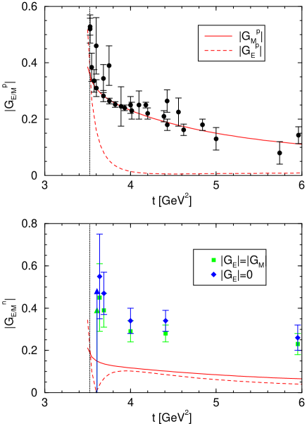
Figure 2: Fit 2 to both spacelike and timelike data for timelike momentum transfer. Vertical dotted line indicates nucleon-antinucleon threshold. Solid lines show $|G_{M}|$, dashed lines show $|G_{E}|$. All neutron data are from the FENICE experiment [3].

In Fig. 2 we show the results of fit 2 compared to the world data. Note that all neutron data are from the FENICE experiment [3]. The solid lines show $|G_{M}|$, while dashed lines show $|G_{E}|$. All proton points are for $|G_{M}|$ as discussed above. The proton magnetic form factor is well described by the fit. The FENICE data for the neutron magnetic form factor have been analyzed under both the assumption $|G_{E}|=|G_{M}|$ (squares) and $|G_{E}|=0$ (diamonds). The latter hypothesis is favored by the measured angular distributions [3]. Neither data set can be described by the fit. Even when the experimental uncertainties of the FENICE data are reduced by a factor of 10 or more, the fit cannot be forced through the data. It is possible that the spectral function simply has not enough freedom to account for the FENICE data and additional poles have to be introduced. It is also surprising that the neutron form factor is larger in magnitude than the proton one, as pQCD predicts asymptotically equal magnitudes. In any case, there is interesting physics in the timelike neutron form factors and more data is called for. Finally, it is interesting to note that fit 2 predicts a zero in the neutron electric form factor close to threshold.

4 NUCLEON FORM FACTORS IN ChPT

Chiral perturbation theory (ChPT) is a low-energy effective field theory of the Standard Model. ChPT focuses on the universal, low-energy aspects of the physical system. All sensitivity to short-distance physiscs is captured in a small number of low-energy constants. ChPT allows for a systematic and model-independent calculation of low-energy observables by means of an expansion in small momenta and quark masses. Particularly important is the spontaneously broken chiral symmetry of QCD in the limit of vanishing quark masses, which guarantees that this expansion is well behaved and severely constrains the form of the effective Lagrangian.

The first systematic investigation of nucleon form factors in the relativistic version of ChPT was given in Ref. [16]. This approach, however, has problems with the expansion in small momenta since the momenta of the nucleons always contain the large nucleon mass. If one uses a nonrelativistic formulation for heavy nucleons, this problem can be circumvented. This Heavy Baryon ChPT is generally very successful for one-nucleon observables. The nucleon form factors were studied within HBChPT in Refs. [17]. It was found that the chiral description already breaks down at relatively small momentum transfers of $-t=Q^{2}\sim 0.2$ GeV². Furthermore, the nonrelativistic expansion does not reproduce the correct singularity structure of the isovector spectral functions. This problem can be overcome in the recently proposed “infrared regularization” of Ref. [18], which is manifestly Lorentz-invariant. Since it is relativistic, this approach keeps the correct singularity structure in the low-energy domain and is expected to improve convergence of the chiral expansion as well. Recently, this method was applied to the electromagnetic form factors of the nucleon by Kubis and Meißner (KM) [8]. In the remainder of this section, we briefly review their results.

Fig. 3 shows the electric form factor of the neutron obtained by KM in relativistic ChPT using infrared regularization.

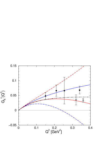
Figure 3: $G_{E}^{n}$ in relativistic ChPT (solid lines) to third (upper curve) and fourth order (lower curve). For comparison: heavy baryon approach (lower/upper dashed line: third/fourth order), dispersion analysis (dot–dashed curve), and some recent experimental points [19].

For comparison, the heavy baryon result and the dispersion analysis discussed above (which can be taken as a representation of the world data) are also shown. The data points are from recent polarization experiments [19]. The relativistic ChPT clearly improves over the heavy baryon calculation, which already breaks down around $Q^{2}=0.1$ GeV². The resummation of the $1/M$ terms in the relativistic approach includes recoil corrections and considerably improves the convergence of the expansion [8].

In the case of the large dipole like form factors $G_{M}^{n}$, $G_{E}^{p}$, and $G_{M}^{p}$, however, the relativistic method does not give an improvement over the heavy baryon expansion. These form factors contain large curvature terms that are not reproduced up to fourth order in the chiral expansion. It is well known that vector mesons contribute significantly to the nucleon form factors and generate the missing curvature terms. In ChPT these contributions are captured in the low-energy constants. The curvature terms, however, only appear in higher orders in the chiral expansion. Since the vector meson couplings to the nucleon are known from the dispersion analysis described above [6, 7], it is both reasonable and economical to include dynamical vector mesons in the theory as no unknown low-energy constants enter. Following this spirit, KM include the $\rho(770)$, $\omega(782)$, and $\phi(1020)$ as dynamical fields using the technology of antisymmtric tensor fields (see Ref. [8] for details). Using the mechanism of resonance saturation, the low-energy constants in the theory without vector mesons $L_{i}$ are split into a vector meson contribution plus a small remainder $\tilde{L}_{i}$ which has to be refit,

$$L_{i}\to\tilde{L}_{i}+\sum_{V}\frac{a_{i}^{V}}{m_{V}^{2}-t}\,.$$ (17)

Keeping the full $t$-dependence in the vector meson contribution amounts to resumming a selected class of higher order diagrams in the chiral expansion. Fig. 4 shows the results for $G_{M}^{n}$

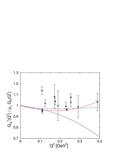
Figure 4: $G_{M}^{n}$ normalized to the dipole fit in relativistic ChPT including vector mesons (solid lines) to third (lower curve) and fourth order (upper curve). For comparison: world data (cf. Refs. [6, 7]) and dispersion analysis (dot–dashed curve).

obtained by KM using this method. Their curves compare well with the world data and the dispersion result. KM find that the validity of the chiral expansion can be extended up to $Q^{2}\approx 0.4$ GeV² using this partial resummation. Similar results hold for the other two dipole-like form factors $G_{M}^{p}$ and $G_{E}^{p}$. Furthermore, the good agreement for $G_{E}^{n}$ is not destroyed by the inclusion of vector mesons.

To summarize, Kubis and Meißner have shown that one can obtain an accurate description of all four nucleon form factors up to $Q^{2}\approx 0.4$ GeV² within the framework of relativistic ChPT and dynamical vector mesons [8]. An extension of this work to $SU(3)$ can be found in Ref. [20].

5 CONCLUSIONS

Dispersion theory and ChPT are two successful approaches to the em form factors of the nucleon that mutually complement each other. Dispersion theory consistently describes the form factors over the whole range of momentum transfers in both the spacelike and timelike regions, while ChPT gives a model independent description at low spacelike $t$ that explicitly incorporates chiral symmetry. The work of KM shows the promise of extending the chiral description to higher momentum transfers by merging dispersive methods and ChPT [8].

The neutron form factors in the timelike region show some interesting features [3]. In particular, the magnitude of the neutron form factors close to the nucleon-antinucleon threshold is larger than expected and at present cannot be described by dispersion theory. More precise data for the em form factors of the nucleon in the timelike region is called for.

6 ACKNOWLEDGEMENTS

I thank R.J. Furnstahl and U.-G. Meißner for a careful reading of the manuscript and B. Kubis and U.-G. Meißner for providing their figures. This work was supported under NSF Grant No. PHY–9800964.

References

- [1] Th. Udem et al., Phys. Rev. Lett. 79 (1997) 2646.
- [2] SAMPLE collaboration, Science 290 (2000) 2115; HAPPEX collaboration, Phys. Rev. Lett. 82 (1999) 1096.
- [3] A. Antonelli et al., Nucl. Phys. B 517 (1998) 3.
- [4] G.F. Chew et al., Phys. Rev 110 (1958) 265; P. Federbush, M. Goldberger, and S. Treiman, Phys. Rev. 112 (1958) 642.
- [5] G. Höhler et al., Nucl. Phys. B 114 (1976) 505.
- [6] P. Mergell, U.-G. Meißner, and D. Drechsel, Nucl. Phys. A 596 (1996) 367.
- [7] H.-W. Hammer, U.-G. Meißner, and D. Drechsel, Phys. Lett. B 385 (1996) 343.
- [8] B. Kubis and U.-G. Meißner, Nucl. Phys. A 679 (2001) 698.
- [9] I. Sabba-Stefanescu, J. Math. Phys. 21 (1980) 175.
- [10] W.R. Frazer and J.R. Fulco, Phys. Rev. 117 (1960) 1603, ibid. 117 (1960) 1609.
- [11] G. Höhler and E. Pietarinen, Phys. Lett. B 53 (1975) 471.
- [12] V. Bernard, N. Kaiser and U.-G. Meißner, Nucl. Phys. A 611 (1996) 429.
- [13] S. Kopecky et al., Phys. Rev. Lett. 74 (1995) 2427.
- [14] S.J. Brodsky and G.P. Lepage, Phys. Rev. D 22 (1980) 2157.
- [15] S. Platchkov et al., Nucl. Phys. A 510 (1990) 740.
- [16] J. Gasser, M.E. Sainio, and A. Svarc, Nucl. Phys. B 307 (1988) 779.
- [17] V. Bernard et al., Nucl. Phys. B 388 (1992) 315; V. Bernard et al., Nucl. Phys. A 635 (1998) 121; (E) 642 (1998) 563.
- [18] T. Becher and H. Leutwyler, Eur. Phys. J. C 9 (1999) 643.
- [19] T. Eden et al., Phys. Rev. C 50 (1994) R1749; M. Meyerhoff et al., Phys. Lett. B 327 (1994) 201; C. Herberg et al, Eur. Phys. J. A 5 (1999) 131; I. Passchier et al., Phys. Rev. Lett. 82 (1999) 4988; M. Ostrick et al., Phys. Rev. Lett. 83 (1999) 276; J. Becker et al., Eur. Phys. J. A 6 (1999) 329.
- [20] B. Kubis and U.-G. Meißner, Eur. Phys. J. C 18 (2001) 747.