Chiral corrections to baryon properties with composite pions
P.J.A. Bicudo
Departamento de Física and CFIF-Edifício Ciência,
Instituto Superior Técnico
Avenida Rovisco Pais, 1096 Lisboa Codex, Portugal
G. Krein
Instituto de Física Teórica, Universidade Estadual Paulista
Rua Pamplona, 145 - 01405-900 São Paulo, SP, Brazil
J.E.F.T. Ribeiro
Departamento de Física and CFIF-Edifício Ciência,
Instituto Superior Técnico
Avenida Rovisco Pais, 1096 Lisboa Codex, Portugal
Abstract
A calculational scheme is developed to evaluate chiral corrections to
properties of composite baryons with composite pions. The composite baryons
and pions are bound states derived from a microscopic chiral quark model.
The model is amenable to standard many-body techniques such as the BCS and
RPA formalisms. An effective chiral model involving only hadronic degrees
of freedom is derived from the macroscopic quark model by projection onto
hadron states. Chiral loops are calculated using the effective
hadronic Hamiltonian. A simple microscopic confining interaction is used
to illustrate the derivation of the pion-nucleon form factor and the
calculation of pionic self-energy corrections to the nucleon and
masses.
pacs:
13.75.Gx, 12.39.Fe, 12.39.Ki, 24.85.+p
I Introduction
The incorporation of chiral symmetry in quark models is an important issue
in hadronic physics. The subject dates back to the early works
[1, 2, 3, 4, 5, 6] aimed at restoring
chiral symmetry to the MIT bag model [7]. The early attempts were
based on coupling elementary pion fields directly to quarks. A great variety
of chiral quark-pion models have been constructed since then and the subject
continues to be of interest in the recent literature [8, 9, 10].
Despite the long history, there are many important open questions in
this field. In the present paper, we are concerned with one of such
questions, namely the coupling of the pion as a quark-antiquark bound state
to the baryons. Starting from a model chiral quark Hamiltonian, we construct
an effective low-energy chiral pion-baryon Hamiltonian appropriate for
calculating chiral loop corrections to hadron properties. The composite
pion and baryon states are determined by the same underlying quark chiral
dynamics.
The model we use belongs to a class of quark models inspired in the
Coulomb gauge QCD Hamiltonian [11] and generalizes the
Nambu–Jona-Lasinio model [12] to include confinement and asymptotic
freedom. This class of
models is amenable to standard many-body techniques such as the BCS formalism
of superconductivity. The initial studies within these models were aimed at
studying the interplay between confinement and dynamical chiral symmetry
breaking (DSB), and concentrated on critical couplings [13]
for DSB and light-meson spectroscopy [14]. The model has
been extended to study the pion beyond BCS level and meson resonant decays in
the context of a generalized resonating group method [15].
Since the model is formulated on the basis of a Hamiltonian, it provides a
natural way to study finite temperature and chemical potential quark
matter [16]. The model and the many-body techniques to solve
it make direct contact with first-principle developments such as
nonperturbative renormalization-group treatments of the QCD
Hamiltonian [17] and Hamiltonian lattice QCD [18].
One important development of the model, in the context of the present paper,
was its extension in Ref. [19] to baryon structure.
In Ref. [19]
a variational calculation was implemented for the masses of baryons and it was
shown that a sizeable - mass difference is obtained from the
same underlying hyperfine interaction that gives a reasonable value for
the - mass difference. This hyperfine interaction, along with
other spin-dependent interactions like tensor and spin-orbit, stem from
Bogoliubov-Valatin rotated spinors that depend on the “chiral angle”. The
chiral angle gives the extent of the chiral condensation in the vacuum and
determines the chiral condensate. The very same variational
wave function was used later for studying -wave kaon-nucleon [20]
scattering and the repulsive core of the nucleon-nucleon force [21].
Both calculations obtain -wave phase-shifts that compare reasonably well
with experimental data. A remarkable feature of all these results for the
low-lying spectrum of mesons and baryons and -wave scattering phase-shifts
is that they are obtained with a single free parameter, the strength of the
confining potential.
In the present paper we go one step forward in the development of the model
and set up a calculational scheme to treat chiral corrections in hadron
spectroscopy. In a recent publication [22], two of us
have calculated the pion-nucleon coupling constant in this model and obtained
reasonable agreement with its experimental value. Here, we are interested in
developing a scheme for calculating chiral corrections to hadron properties.
We study the requirements to obtain in the context of the model the correct
leading nonanalytic behavior (LNA) of chiral loops. Our scheme follows the
standard practice [6] [23] of constructing an effective
baryon-pion Hamiltonian by projecting the quark Hamiltonian onto a
Fock-space basis of single composite hadronic states. Chiral loop
corrections are then calculated with the effective Hamiltonian in
time-ordered perturbation theory. The difference here is that while in the
previous works the pion is an elementary particle, in our approach the pions
are composites described by a Salpeter amplitude.
A difficulty appears in the implementation of the projection of the
microscopic quark Hamiltonian onto the composite hadron states, which is
not present when the pion is treated as an elementary particle. The
difficulty is related to the two-component nature of the Salpeter amplitude
of the pion. The two components correspond to positive and negative energies
(forward and backward moving, in the language of of time-ordered perturbation
theory), they are 2 2 matrices in spin space and are called
energy-spin (E-spin) wave functions. For the pion, the negative-energy
component is as important as the positive-energy one – in the chiral
limit they are equal – because of the Goldstone-boson nature of the pion.
Because of this, the Fock-space representation of the pion state is not
simple. We overcome the difficulty by rephrasing the formalism of the
Salpeter equation in terms of the RPA (random-phase approximation) equations
of many-body theory. The single-pion state is obtained in terms of a
creation operator acting on the RPA vacuum. The pion creation operator is a
linear combination of creation and annihilation operators of pairs of
quark-antiquark operators; the positive-energy Salpeter component comes
with the creation operator of the quark-antiquark pair, and the
negative-energy one comes with the annihilation operator of the
quark-antiquark pair. In this way, the projection of the microscopic
quark Hamiltonian onto the single hadron states becomes feasible and simple.
The paper is organized as follows. In the next Section we review the basic
equations of the model. We show the relationship of the formalisms of the
Salpeter equation and of the many-body technique of the RPA.
In Section III we derive the pion-baryon vertex function in terms
of the bound-state Salpeter amplitudes for the pion and the baryon. We obtain
an expression that is valid for a general microscopic quark interaction, not
restricted to a specific form of the potential. Given the pion-baryon vertex
function, we derive the expression for the baryon self-energy correction in
Section IV. Although the derivation of the expression for
the self-energy is well-known in the literature, we repeat it here to make
the paper easier to read. In Section V we obtain numerical
results for the pion-baryon form factor and coupling constants. Numerical
results and the discussion of the LNA contributions to the baryon masses are
presented in Section VI. Section VII presents
our conclusions and future directions.
II The model
The Hamiltonian of the model is of the general form
(1)
where is the Dirac Hamiltonian
(2)
with the Dirac field operator, and a chirally
symmetric four-fermion interaction
(3)
Here, are the generators of the color
SU(3) group, is one, or a combination of Dirac matrices, and
contains a confining interaction and other spin-dependent
interactions. One example of will be presented in
section V, when we make a numerical application of the
formalism.
Once the model Hamiltonian is specified, the next step consists in
constructing an explicit but approximate vacuum state of the Hamiltonian
in the form of a pairing ansatz. This is most easily implemented in the
form of a Bogoliubov-Valatin transformation (BVT). The transformation
depends on a pairing function, or chiral angle that determines
the strength of the pairing in the vacuum. The quark field operator is
expanded as
(4)
where the quark and antiquark annihilation operators and annihilate
the paired vacuum, or BCS state, . Here the spinors
and depend upon the chiral angle as
(5)
(6)
where and are the spinor eigenvectors of Dirac matrix
with eigenvalues , respectively.
The chiral angle can be determined from the minimization of the vacuum
energy density,
(7)
(8)
where is the trace over color, flavor, and Dirac indices,
and
(9)
The minimization of the vacuum energy leads to the gap equation,
(10)
with
(11)
(12)
where is the Fourier transform of ,
(13)
The pion bound-state equation is given by the field-theoretic Salpeter
equation. The wave function has two components, and , the
positive- and negative-energy components. Each of the ’s is a
matrix in spin space, and .
For this reason, the ’s are also called energy-spin (E-spin)
wave functions. The ’s satisfy the following coupled integral equations:
(14)
(15)
where , and the kernel is
given by
(16)
(17)
Here, the super-script on means spin-transpose of ,
. The amplitudes are normalized as
(18)
In the language of many-body theory, these equations can be identified with
the RPA equations [24]. In the RPA formulation, one writes for the
one-pion state (suppressing isospin quantum numbers)
(19)
where is the RPA vacuum, which contains correlations
beyond the BCS pairing vacuum , and
is the pion creation operator
(20)
where the were defined above. In this formulation,
Eqs. (14) and (15) above are obtained from the RPA equation
of motion:
(21)
The normalization is such that
(22)
The verification of DSB consists in finding nontrivial solutions to the
gap equation, Eq. (10), and the existence of solutions for the pion
wave function. Refs. [11] and [15] show that for a
confining force, there is always a nontrivial solution for the gap and pion
Salpeter equations. Moreover, good numerical values are obtained for the
chiral parameters such as the pion decay constant and the chiral condensate
when an appropriate spin-dependent potential is used [25].
The inclusion of RPA correlations beyond BCS pairing was shown in
Ref [24] to have a dramatic effect on the mass spectrum of the
pseudo scalar mesons ( and ), while it has almost no effect on
the mass spectrum of vector mesons ( and ). One can trace this
effect to the fact that the pseudo scalar mesons have a sizeable “negative
energy” component wave function, while the vector mesons have a very
small negative energy component [15]. For baryons (such as
nucleon and ), since they do not have a sizeable negative energy
component [19], one expects that they can be reliably obtained
from the BCS vacuum. We write therefore for the one-baryon state
(23)
where the baryon creation operator is given by
(24)
(25)
Here is the Levi-Civita tensor, which guarantees
that the baryon is a color singlet and are the
spin-isospin coefficients. The wave function
is determined variationally [19]. The index on the baryon
operators indicates a bare baryon, i.e. a baryon without pion cloud
corrections.
The important fact to notice here is that the baryon wave function depends
on the chiral angle and as such, spin splittings and other
properties are determined by the same physics that determines vacuum
properties. The pion-baryon vertex, that we will discuss in the next
section, will therefore depend on the chiral angle not only because
of the pion, but also because of the baryon wave function. Numerical
results for the masses of the the nucleon and have been
obtained previously [19] and are of the right order of magnitude
as compared with experimental values. Of course, fine-tuning with different
spin-dependent interactions can improve the numerical values of the
calculated quantities.
III Pion-baryon vertex function
We obtain an effective baryon-pion Hamiltonian by projecting the model
quark Hamiltonian onto the one-pion and one-baryon states, Eqs. (19)
and (23). We use a shorthand notation. For the bare baryons, i.e.
baryons without pionic corrections, we use the indices to indicate all the quantum numbers necessary to specify
the baryon state, such as spin, flavor and center-of-mass momentum.
For the pion, we use to specify all the quantum numbers
of the pion state. With this notation, the effective Hamiltonian
can be obtained as
(26)
(27)
This leads to an effective Hamiltonian that can be written as the sum of the
single-baryon and single-pion contributions, and the pion-baryon vertex:
(28)
where contains the single-baryon and single-pion
contributions
(29)
and is the pion-baryon vertex
(30)
Here, and ( and
) are the baryon (pion) creation and annihilation operators, discussed
in the previous section. Note that we have assumed that states with different
quantum numbers are orthogonal. Note also that in writing the state
we have implicitly assumed that the negative-energy component
of the baryon is negligible and the baryon creation operator acting on the
RPA vacuum has the same effect as acting on the BCS vacuum.
We note that the projection of the microscopic quark Hamiltonian to an
effective hadronic Hamiltonian can be obtained in a systematic and controlled
way using a mapping procedure [26]. We do not follow such a procedure
here because we are mainly concerned with tree-level pion-baryon
coupling and the projection we are using is enough to obtain the desired
effective coupling. For processes that involve quark-exchange, such as
baryon-meson or baryon-baryon interactions, a mapping procedure would be
useful. In a future publication, we intend to address such processes in the
context of the present model.
The single-hadron Hamiltonians and give
(31)
with and in the
rest-frame. The vertex gives the coupling of the pion to the baryon and,
as we will show later, leads to loop corrections to the baryon self-energy.
The pion-nucleon vertex function can be written generally as
(32)
where the ’s are of the general form (for simplicity we suppress
the color and spin-flavor wave functions in the following)
(33)
where the ’s involve the Dirac spinors and the pion wave
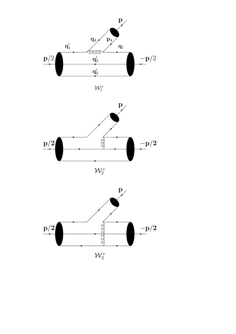
functions. In Figure 1 we present a pictorial representation of the different
contributions to the vertex function. Explicitly, the ’s
are given by
(34)
(35)
(36)
(37)
(38)
(39)
In these formulas, the quark momenta in the initial (final) nucleon
() and the momenta of the quark
and antiquark in the pion, and , are expressed in terms
of the loop momenta by momentum conservation (see
Fig. 1) .
Once the effective baryon-pion Hamiltonian is obtained, one can calculate
the pionic corrections to baryon properties as in the CBM and in the
traditional Chew-Low model. This will be done in the next section.
Before leaving this section, we recall that the use of the Breit frame is
essential in calculations of form factors (vertex functions) in static
models [27], like the present one. This is true
for composite models for which approximate solutions that maintain
relativistic covariance are very difficult to implement. This was the
case for all old, static source, pion-nucleon models like the
Chew-Low model [28]. In particular, as explained in
Ref. [27], electromagnetic gauge invariance is respected in
this frame. Therefore, in calculating loop corrections to baryon properties,
we employ the Breit-frame vertex functions. In the Breit frame, we denote
the incoming pion and nucleon momenta by and , respectively,
and the outgoing nucleon momentum by . In this frame, the internal
momenta of quarks and antiquarks are given in terms
of the loop momenta and as
(40)
(41)
(42)
for the vertex and
(43)
(44)
(45)
for the vertex . In following equations, we also denote the
vertex function as .
IV Self-energy correction to baryon masses
For completeness we review the derivation of the expression for the
self-energy correction from the effective baryon-pion Hamiltonian
of Eq. (28) in the “one-pion-in-the air”
approximation [28, 6]. The baryon self-energy is defined
as the difference of bare- and dressed-baryon energies:
(46)
The physical baryon mass is given by the (in general, nonlinear)
equation
(47)
where is the bare baryon mass (i.e. without pionic corrections)
and is the self-energy function.
Let denote the physical baryon state, and the “bare”
undressed state. Let be the probability of finding in
. Then one can write
(48)
where is a projection operator that projects out the component
from ,
(49)
We have that
(50)
(51)
We can now express in terms of and the pion-baryon
interaction Hamiltonian as
(52)
On the other hand, since
(53)
we have that the self-energy is given by
(54)
(55)
This expression can be further approximated so as to avoid solving
complicated integral equations for the self-energy. We can manipulate the
expression for to obtain (for details, see Ref. [6]):
(56)
with
(57)
The approximation consists in absorbing into such that
(58)
with
(59)
where and are the physical energies. Therefore,
the baryon self-energy can be written as
(60)
Finally, insertion of a sum over intermediate baryon-pion states in
Eq. (60) leads to
(61)
The structure vertex-propagator-vertex
in Eq. (60) is an effective baryon-pion interaction. The main
difference here with the hybrid
approaches [1, 2, 3, 4, 5, 6] is that we do not
have a point-like pion coupling to point-like quarks and antiquarks. The
pion-baryon vertex arises through the “Z-graphs” in which the antiquark of
the pion is annihilated with a quark of the “initial” baryon and the quark
of the pion appears in the “final” baryon. Therefore, the vertex function
incorporates not only the extension of the baryons, but also the extension of
the pion.
We truncate the sum over the intermediate states in Eq. (61) to the
lowest mass states, namely the nucleon and the . In this case,
we obtain for the on-shell and self-energies the coupled
set of equations
(62)
(63)
This is the final result for the pion loop correction for the nucleon
and .
One important consequence of projecting the microscopic quark interaction
onto hadronic states is that the leading nonanalytic (LNA) contributions in
the pion mass as predicted by chiral perturbation theory are correctly
obtained [9]. In particular, as we discuss in the next section,
Eq. (62) leads to an LNA contribution to the
nucleon mass as predicted by QCD [29], namely
(64)
In models where the pion is treated as a point like particle, this result
follows trivially [9] from Eq. (62). In the context of the
present model, where the pion is not treated covariantly, such a result does
not follow in general for an arbitrary interaction. The difficulty is related
to the fact the the pion dispersion relation,
, is not obtained in general in a
noncovariant model. In the CBM for example, the pion is point like and the
normalization is correct from the very beginning. However, the microscopic
quark interaction can be chosen such that the pion dispersion relation is
correctly obtained [14, 25]. These issues will be discussed
in Section VI.
V The pion-nucleon and pion- form factors
Our aim is to obtain an estimate for the numerical values of the
pionic self-energies. It happens that nature has produced a
sort of low energy filter (chiral symmetry) for the details of strong
interactions. Indeed it is remarkable that although intermediate theoretical
concepts like gluon propagators, quark effective masses and so on, might
vary (in fact they are not gauge invariant and hence they are not physical
observables), chiral symmetry contrives for the final physical results, e.g.
hadronic masses and scattering lengths, to be largely insensitive to the above
mentioned theoretical uncertainties. The pion mass furnishes the ultimate
example: In the case of massless quarks, the pion mass is bound to be zero,
regardless of the form of the effective quark interaction provided it
supports the mechanism of spontaneous breakdown of chiral symmetry.
The other example is provided by the scattering
lengths [30] which are equally independent of the form of the
quark kernel[31]. Furthermore it has become more and more
evident through the accumulation of theoretical calculations on low energy
hadronic phenomena, ranging from calculations on Euclidean space to
instantaneous approximations and from harmonic kernels to linear confinement,
that low energy hadronic phenomenology only seems to depend mildly on the
details of the quark kernels used. To this extent, we will use for the
quark-quark interaction a kernel of the form,
(65)
(66)
where is a free parameter. This potential has been widely used
in the context of chiral symmetry breaking because it allows a great
deal of simple analytic calculations (which is not the case for the linear
potential). The harmonic potential basically differs from the linear
potential in domains of the baryon-pion-baryon overlap kernel which contribute
little to the total geometrical overlap so that, at least for results
proportional to these overlaps, they should not differ too much.
The momentum-dependent part of the Salpeter amplitude for the baryon,
in Eq. (25), is taken to be of a
Gaussian form
(67)
where is the variational parameter and is the
normalization. Notice that since the integrations of the quark momenta in
the functions in Eq. (33) are made through a Monte Carlo
integration, the Gaussian ansatz is not essential and does not simplify our
calculations, but we still use it to make contact with previous calculations.
As in our previous calculation [22] for the pion-nucleon coupling
constant, the Salpeter amplitudes up to first
order in are given by
(68)
(69)
where is the chiral angle and is the first-order
correction to the pion energy. The normalization is
proportional to and is given as
(70)
The energy is given in terms of the second derivatives of the
diagonal components of the Salpeter kernel with respect to and its
explicit form is given in Eq. (24) of Ref. [22]. Note that the
truncation up to first order in of the Salpeter amplitude
constitutes a reasonable approximation due to the fact that c.m.
momenta-dependent distortions of the pion and nucleon wave functions are
geometrically damped because of the geometric overlap kernel
integrations for the functions in Eq. (33) –
see Ref. [32]. Explicit numerical solutions were obtained in
Ref. [22] for the functions and .
For completeness, we initially repeat the results of Ref. [22] for
the coupling constants and .
In Ref. [22], they were obtained as
(71)
(72)
where the isospin matrix is omitted and
(73)
where means integration over and (see
Eq. (33) ) and the set of functions is
given by,
(74)
(75)
(77)
(79)
Here, stand for the baryon in and out Salpeter
amplitudes and represent the pion Salpeter amplitudes.
The baryon-pion coupling constants are obtained as the zero limit of the
nucleon (or ) momentum, , of the above overlap
functions. For simplicity, we are defining the couplings at zero momentum,
and not at the physical pion mass. In order to facilitate the integration, in
Ref. [22] a Gaussian parameterization for the
and was used. Here, since we need the vertex
function for , we use a Monte Carlo integration to perform the
multi dimensional integral that gives the overlap function and use the full
numerical solution for the gap function (not the Gaussian parameterization).
We first checked the correctness of our Monte Carlo integration with
the result of Ref. [22] for the special case of using the
same Gaussian parameterization as was used there. This was done by calculating
for and finding the limit of
when to obtain
.
As in Ref. [22] we have used MeV for the
strength of the potential. The variational determination of of
the baryon amplitude, Eq. (67), leads to . For
the , the result is not much different and therefore we use
.
Introducing the quantities
(80)
we can summarize the couplings of the pion to the nucleon and
as follows:
(81)
For the value of given above, we have .
The numerical values for the couplings are then
(82)
The effect of the Gaussian parameterization can be assessed by comparing
with the corresponding numbers of Ref. [22]. For example,
and in Ref. [22];
the effect of the parameterization is therefore of the order of 20.
Next, we calculated the full overlap function for . In
Figure 2 we plot the function
for the parameters given above. It is instructive to compare the momentum
dependence of this form factor with the one given by the
CBM [6, 23]:
(83)
where is the spherical Bessel function and is the radius of the
underlying MIT bag. The solid line is our result and the dashed one is
the CBM result for fm. The faster falloff of our result is
clearly a consequence of our Gaussian ansatz. As we will discuss soon,
this rapid falloff will have the consequence of giving a smaller
value of the self-energy correction to the nucleon mass, as compared to
the corrections obtained with the CBM.
VI Self-energy corrections to the nucleon and masses
In this Section we present numerical results for the pionic
self-energy corrections to the nucleon and masses
and discuss the LNA contribution to the masses. We start by
rewriting the vertex function in a manner to make clear the problem
with the pion dispersion relation. The pion energy is given,
for low , as [14, 25]
(84)
where
(85)
The point is that for an arbitrary quark-quark interaction one
obtains in general two different values for the pion decay constant,
and (the explicit calculations can be
found in Refs. [14, 25]), depending on how one
defines the decay constant. When using the time component of the axial
current, one obtains , and when using the space component
one obtains . However, as suggested in
Ref. [14], and explicitly demonstrated in Ref. [25],
this problem can be cured by adding a transverse gluon interaction.
Therefore, to illustrate the point of obtaining the correct LNA term from
Eq. (62) with composite pions, we use the correct pion dispersion
relation and assume and
denote .
The normalization of the pion Salpeter amplitude, Eq. (70),
can be rewritten as
(86)
That is, from Eq. (70) is . We next extract
from the vertex function (we concentrate on the NN form factor) this
normalization in the following way
(87)
The relation of the function to the overlap function
can be trivially obtained by comparing with
Eq. (71).
Inserting Eq. (87) in the expression for the and
self-energies, Eqs. (62) and (63), and after performing
rather straightforward spin-isospin algebra one obtains
(88)
(89)
where
(90)
and
(91)
Note that in principle we have different spatial dependencies for the ,
, vertices, but for simplicity we have written them here as
being equal. A schematic representation of Eqs. (88) and
(89) is presented in Fig. 3. It is important to note that
these equations are not the ones one would obtain by simple perturbation
theory; they are actually nonperturbative, because of the dependence on
on the r.h.s.
It is easy now to obtain the LNA contributions to the masses [9]. For
the nucleon, the LNA contribution comes from the first term in Eq. (88)
by performing the integral. The integral can be done by transforming it into a
contour integral and making use of Cauchy’s theorem. The result is
Eq. (64). For the , the LNA contribution follows in a similar
way from the last term in Eq. (89).
To conclude, we discuss numerical results for the pionic corrections.
Initially we solve variationally the bare nucleon case. As discussed above,
using MeV, we obtain for the variational size parameter the value
. We also use here . This
leads to the following values for the bare and masses
(92)
The difference between the masses, of the order of MeV, comes from the
hyperfine splitting induced by the confining interaction. Given these values,
we solve the two self-consistent equations given in Eqs. (88) and
(89). They are solved by iteration. We obtain for the masses
(93)
Comparing with the values above, we see that the pionic effect is relatively
small, as it should be, and of the order of MeV for the
and MeV for the . The pionic effect is smaller for the
, as one expects from spin-isospin considerations [9]. The
results obtained with the CBM for a fm are a bit larger [23].
The difference can be traced to the rapid falloff of the form factor in our
model.
We certainly do not expect these numbers to be definitive. Once more realistic
microscopic quark interactions and ansatze for the baryon wave function are
used, they might be improved. However, independently of the microscopic model,
our scheme is general and able to incorporate such interactions and new
baryon amplitudes. I would be of particular interest to have the numbers for a
linear confining interaction with short range gluonic interactions that
respect asymptotic freedom.
VII Conclusions and future perspectives
We developed a calculational scheme to calculate chiral loop corrections to
properties of composite baryons with composite pions. The composite baryons
and pions are bound states derived from a microscopic chiral quark model
inspired in Coulomb gauge QCD and provides a generalization of the
Nambu–Jona-Lasinio model to include confinement and asymptotic freedom.
An effective chiral hadronic model is constructed by projecting the
microscopic quark Hamiltonian onto a Fock-space basis of single composite
hadronic states. The composite pions and baryons are obtained from the same
microscopic Hamiltonian that describes the chiral vacuum condensate. The
projection of the quark Hamiltonian onto the pion states is nontrivial
because of the two-component nature of the Salpeter amplitude of the pion.
As explained before, the two components correspond to positive and
negative energies which complicates the Fock-space representation of the pion
state. The projection is made possible by rephrasing the formalism of the
Salpeter equation in terms of the RPA equations.
The development of models and calculational methods of the sort described
in the present paper are relevant in the context of a phenomenological
understanding of nonperturbative phenomena of strong QCD like confinement and
dynamical chiral symmetry breaking. Eventually full lattice QCD simulations
aimed at studying hadronic structure will be available and phenomenological
models will play a central role in the interpretation of the data generated.
The developments of the present paper are of particular interest for the
first-principle developments based on the QCD Hamiltonian, such as the
nonperturbative renormalization program for the QCD Hamiltonian [17]
and Hamiltonian lattice QCD [18]. We intend to implement the technique
developed here to such first-principle QCD calculations.
We illustrated the applicability of the formalism with a numerical calculation
using a simple microscopic interaction, namely a confining harmonic potential,
and a simple Gaussian ansatz for the baryon amplitude. This very same -wave
interaction has been used in a variety of earlier calculations, such as
meson and baryon spectroscopy and -wave nucleon-nucleon interaction.
Numerical results were obtained here for the pion-nucleon form factor and
for the pionic self-energy corrections to the nucleon and
masses in the nonperturbative one-loop approximation. Despite the simplicity
of the interaction, the results obtained are very reasonable.
For the future, the most pressing development would be to use a microscopic
interaction that is consistent with asymptotic freedom and describes
confinement by a linear potential. The calculation of the pion wave function
beyond lowest order in momentum must be implemented and the variational ansatz
for the baryon amplitude must be improved. A more ambitious development would
be to include explicit gluonic degrees of freedom. In this case
renormalization issues will show up and the new techniques such as discussed
in Ref. [17] will certainly be useful. Another very interesting
direction would be to employ the techniques developed here in Hamiltonian
lattice QCD.
Acknowledgements.
This work was partially supported by CNPq (Brazil) and ICCTI (Portugal).
The authors thank Nathan Berkovits for reading the manuscript and making
suggestions on the presentation.
REFERENCES
[1] A. Chodos and C.B. Thorn, Phys. Rev. D. 12, 2733
(1975); T. Inoue and T. Maskawa, Prog. Theor. Phys. 54, 1833
(1975).
[2] M.V. Barnhill, W.K. Cheng, and A. Halprin, Phys. Rev.
D 20, 727 (1979).
[3] G.E. Brown and M. Rho, Phys. Lett. 82B, 177
(1979).
[4] V. Vento, M. Rho and G.E. Brown, Nucl. Phys.
A345, 413 (1980).
[5] R.L. Jaffe, Lectures at the 1979 Erice School,
MIT preprint October 1980.
[6] S. Théberge, A.W. Thomas, and G.A. Miller, Phys.
Rev. D 22, 2838 (1980); 23, 2106(E) (1981); A.W. Thomas,
S. Théberge, and G.A. Miller, ibib24, 216 (1981).
[7] A. Chodos, R.L. Jaffe, K. Johnson, C.B. Thorn, and
V.F. Weisskopf, Phys. Rev. D 9, 3471 (1974); A. Chodos, R.L.
Jaffe, K. Johnson, and C.B. Thorn, ibid10, 2599 (1974);
T.A. de Grand, R.L. Jaffe, K. Johnson, and J. Kiskis, ibid12, 2060 (1975).
[9] A.W. Thomas and G. Krein, Phys. Lett. 456B, 5
(1999); ibib481B, 21 (2000).
[10] N. Isgur, “Critique of a Pion Exchange Model for Interquark
Forces”, nucl-th/9908028.
[11] M. Finger, D. Horn, and J.E. Mandula, Phys. Rev. D 20,
3253 (1979); M. Finger, J. Weyers, D. Horn and J.E. Mandula, Phys. Lett.
62B, 1980; A.J.C. Hey and J.E. Mandula, Nucl. Phys. B198, 237
(1980); 3253 (1979); J.R. Finger and J.E. Mandula, ibib, B199,
168 (1982); A. Le Yaouanc, L. Oliver, O. Péne, and J.-C. Raynal, Phys.
Lett. B134, 249 (1984); Phys. Rev. D 1233 (1984); A. Amer,
A. Le Yaouanc, L. Oliver, O. Péne, J.-C. Raynal, Phys. Rev. Lett.
50, 87 (1984); S.L. Adler and A.C. Davis, Nucl. Phys. B224,
469 (1984).
[12] Y. Nambu and G. Jona-Lasinio, Phys. Rev. 122, 345
(1961); ibid124, 246 (1961).
[13] A. Le Yaouanc, L. Oliver, O. Péne, and J.-C. Raynal,
Phys. Rev. D 29, 1233 (1984).
[14] A. Le Yaouanc, L. Oliver, O. Péne, and J.-C. Raynal,
Phys. Rev. D 31, 137 (1985).
[15] P.J.A. Bicudo and J.E.F.T. Ribeiro, Phys. Rev. D 42,
1635 (1990); 42, 1625 (1990); 42, 1635 (1990).
[16] A. Mishra, H. Mishra, and S.P. Misra, Z. Phys. C 59,
159 (1993); A. Mishra, H. Mishra, P.K. Panda, and S.P. Misra, Z. Phys. C
63, 681 (1994).
[17] A.P. Szczepaniak and E.S. Swanson, Phys. Rev. D 55,
1578 (1997); D.G. Robertson, E.S. Swanson, A.P. Szczepaniak, C.-R. Ji,
and S.R. Cotanch, Phys. Rev. D 59, 074019 (1999); E. Gubankova,
C.-R. Ji, S.R. Cotanch, Phys. Rev. D 62 074001 (2000), A.P. Szczepaniak
and E.S. Swanson Phys. Rev. D 62, 094027 (2000).
[18] A. Le Yaouanc, L. Oliver, O. Pène, and J.-C. Raynal,
Phys. Rev. D 33, 3098 (1986); A. Le Yaouanc, L. Oliver, O. Pène,
J.-C. Raynal, M. Jarfi and O. Lazrak, Phys. Rev. D 37, 3691 (1988);
ibid37, 3702 (1988); E.B. Gregory, S.-H. Guo, H. Kröger,
and X.-Q. Luo, Phys. Rev. D 62, 054508 (2000); Y. Umino, Phys. Lett.
492B, 385 (2000); hep-lat/0007356; hep-ph/0101144.
[19] P.J.A. Bicudo, G. Krein, J.E.F.T. Ribeiro, and J.E. Villate,
Phys. Rev. D 45, 1673 (1992).
[20] P. Bicudo, J. Ribeiro, and J. Rodrigues, Phys. Rev. C 52,
2144 (1995).
[21] P. Bicudo, L. Ferreira, C. Placido, and J. Ribeiro, Phys. Rev.
C 56, 670 (1997).
[22] P. Bicudo and J. Ribeiro, Phys. Rev. C 55, 834 (1997).
[24] F.J. Llanes-Estrada and S.R. Cotanch, Phys. Rev. Lett.
84, 1102 (2000).
[25] P.J.A. Bicudo, Phys. Rev. C 60, 035209 (1999).
[26] D. Hadjimichef, G. Krein, S. Szpigel, and J.S. da Veiga,
Phys. Lett. 367B, 317 (1996); Ann. Phys. (NY) 267, 105 (1998);
M.D. Girardeau, G. Krein, and D. Hadjimichef, Mod. Phys. Lett. A11,
1121 (1996).
[27] G.A. Miller and A.W. Thomas, Phys. Rev. C 56, 2329
(1997).
[29] P. Langacker and H. Pagels, Phys. Rev. D 8, 4595 (1973);
D 10, 2904 (1974).
[30] S. Weinberg, Phys. Rev. Lett. 17, 616 (1966).
[31] J.E. Ribeiro, to be published in Proceedings of
IV International Conference on Quark Confinement and the Hadron Spectrum,
Vienna, Austria, 2000 (World Scientific, Singapore).
[32] J.E. Ribeiro, Phys. Rev. D 25, 2406 (1982);
E. van Beveren, Z. Phys. C 17, 135 (1982).
FIG. 1.: Graphical representation of the functions .
FIG. 2.: The function . The solid line is the form factor obtained with
the baryon amplitude of Eq. (67) and pion Salpeter amplitudes of
Eqs. (68) and (69). The dashed line is the CMB form
factor of Eq. (83) for fm.
FIG. 3.: Schematic representation of the pion self-energy corrections to the
nucleon () and delta () masses.