Neutrino anomalies and large extra dimensions

Abstract

Theories with large extra dimensions can generate small neutrino masses when the standard model neutrinos are coupled to singlet fermions propagating in higher dimensions. The couplings can also generate mass splittings and mixings among the flavour neutrinos in the brane. We systematically study the minimal scenario involving only one singlet bulk fermion coupling weakly to the flavour neutrinos. We explore the neutrino mass structures in the brane that can potentially account for the atmospheric, solar and LSND anomalies simultaneously in a natural way. We demonstrate that in the absence of a priori mixings among the SM neutrinos, it is not possible to reconcile all these anomalies. The presence of some structure in the mass matrix of the SM neutrinos can solve this problem. This is exemplified by the Zee model, which when embedded in extra dimensions in a minimal way can account for all the neutrino anomalies.

I Introduction

The present data from the experiments on atmospheric, solar and reactor neutrinos indicate neutrino flavour oscillations. The data from each of these sets of experiments individually can be explained by a single dominating mass square difference $\Delta m^{2}$ and a mixing angle $\theta$. The atmospheric neutrino data [1] indicate $\nu_{\mu}\leftrightarrow\nu_{\tau}$ as the dominant mode, with $\Delta m^{2}_{atm}=(1-8)\cdot 10^{-3}\mbox{ eV}^{2}~{},~{}\sin^{2}2\theta=0.8-1.0$. There is no compelling evidence that the electron neutrinos participate in the oscillations of atmospheric neutrinos. Moreover, the CHOOZ experiment [2] gives an upper bound on the mixing of $\nu_{e}$: we have $\sin^{2}2\theta_{e}\leq 0.1$ where $\nu_{3}$ is the mass eigenstate such that $\Delta m^{2}_{31}\approx\Delta m^{2}_{32}\approx\Delta m^{2}_{atm}$. The three MSW solutions (LMA, SMA and LOW) as well as the vacuum oscillations can provide reasonable fits to the solar neutrino data [3], all these solutions have $\Delta m^{2}_{\odot}\leq 2\cdot 10^{-4}$ eV². The results of the LSND experiment [4] are neither confirmed nor fully excluded by the KARMEN2 data [5], and the combined fit allows a region [6] $\Delta m^{2}_{LSND}=(0.1-1)\mbox{ eV}^{2}~{},~{}\sin^{2}2\theta_{\mu e}\approx 10^{-3}-10^{-2}$.

In the context of only three known neutrino species, the $\Delta m^{2}$s corresponding to the solutions of the three neutrino anomalies (atmospheric, solar and LSND) cannot be reconciled and if the oscillation mechanism is to be used to explain all the anomalies, the introduction of a sterile neutrino becomes necessary. There are two simple schemes of mixing among four neutrinos which can account for all the neutrino anomalies:

(i) In the “3+1” scheme [8], the masses of the three active states are separated from that of the sterile one by the LSND scale. The possible $\nu_{e}-\nu_{\mu}$ oscillations seen at LSND arise through simultaneous mixings of $\nu_{e}$ and $\nu_{\mu}$ with the sterile neutrino $\nu_{s}$. Such a picture is strongly constrained by laboratory disappearance experiments. It was argued [8] that these experiments constrain the $\nu_{e}-\nu_{\mu}$ mixing below the experimental signal at LSND. This has changed with the new LSND data and the 3+1 scheme is claimed [9] to be viable for some parameter range, though the detailed statistical analysis in [10] does not support this claim.

(ii) The second scheme — known as the “2+2” scheme [8, 11] — corresponds to two nearly degenerate pairs of neutrinos separated by the LSND mass scale. The mixings within the pairs account for the solar and atmospheric flux deficits. The small oscillation probability seen in the LSND experiment can be explained by requiring that $\nu_{e}$ and $\nu_{\mu}$ belong to two different degenerate pairs. This implies that the sterile state has significant admixture either with $\nu_{e}$ or $\nu_{\mu}$ and thus plays an important role in generating either the solar or the atmospheric neutrino deficit. The data on atmospheric neutrinos disfavour $\nu_{\mu}-\nu_{s}$ as the dominant source of the $\nu_{\mu}$ oscillations [1]. The global fit to the available sets of the solar neutrino data are also better described in terms of $\nu_{e}$ conversion to active rather than the sterile state, although the latter possibility is not completely ruled out [12]. The 2+2 scheme will be ruled out if both the solar and the atmospheric neutrinos are found to be mainly oscillating to active neutrinos.

It follows that both the above schemes are strongly constrained and may not prove adequate for incorporating the LSND signal. In this case, the description of data in terms of four neutrino mixing would be challenged and more complicated possibilities would be needed. Quite apart from phenomenological incompatibility, the very existence of a light sterile state needs theoretical justification. While there have been attempts in this direction [13], the introduction of more than one light sterile states can add to theoretical difficulties.

The above theoretical and phenomenological problems find natural solutions in theories with extra dimensions of mm size [14]. Firstly, such theories can provide justification for the existence of light sterile states which form a part of the Kaluza Klein (KK) tower associated with a singlet fermion residing in the bulk volume of the full higher dimensional theory. In addition, the presence of more than one light sterile state allows additional phenomenological possibilities not envisaged in the context of the 2+2 or 3+1 schemes mentioned above. As a result, these theories provide a potentially useful framework for understanding all neutrino anomalies.

The standard model particles are assumed to be confined to a three-brane embedded in a higher dimensional bulk. The gauge singlet states are not confined this way and propagate in the bulk. Such theories have been argued to provide some understanding of neutrino masses if one assumes the presence of a singlet neutrino $\nu_{B}$ propagating in the bulk. The couplings of $\nu_{B}$ to the flavour states residing in bulk are suppressed by a volume factor corresponding to the extra dimensions and lead to very small neutrino masses [15, 16] in spite of the new physics at TeV scale.

The minimal approach consists of assuming only five dimensions and the presence of only one bulk neutrino coupling to all the known flavors through

$${m_{\alpha}\over v}\bar{l_{\alpha}}\phi\nu_{B}+h.c.~{},$$ (1)

where

$$m_{\alpha}\equiv{h_{\alpha}vM_{f}\over M_{P}}\approx 6\cdot 10^{-5}\,{\rm eV}h_{\alpha}\left({M_{f}\over\,{\rm TeV}}\right)\quad.$$ (2)

Here $h_{\alpha}$ is the Yukawa coupling, and $M_{f}(M_{P})$ is the fundamental (Planck) mass scale. Neutrino masses and mixings are determined by four parameters: three mixing parameters $\xi_{\alpha}\equiv\sqrt{2}m_{\alpha}R$ and an overall mass scale $m^{2}\equiv m_{e}^{2}+m_{\mu}^{2}+m_{\tau}^{2}$.

From the point of view of the 4-dimensional theory, the $\nu_{B}$ residing in a five dimensional world contains a massless state which can provide a sterile neutrino needed to understand various neutrino anomalies. The $n^{\rm th}$ KK excitation associated with $\nu_{B}$ has a mass $m_{n}=n/R$. For $R\sim 0.1~{}mm$, masses of some of the low lying excitations would be in the range needed for the occurrence of the MSW resonance for solar neutrinos. The mixing of the KK states with $\nu_{e}$ is governed by $\xi_{e}$. For $M_{f}$ in the TeV range, this mixing is in the range needed for the small mixing angle solution of the solar neutrino problem. Hence, the MSW solution in this context is correlated to observable extra dimensions and TeV mass scale [17]. However, these values of the parameters cannot provide the atmospheric neutrino scale if Yukawa couplings $h_{\alpha}<1$. This makes it difficult to reconcile all the neutrino anomalies and one needs to go beyond this minimal picture. The following different possibilities have been considered in the literature:

(i) Extension of the minimal scheme with three bulk neutrinos was considered in [18]. The phenomenology of this case is described in terms of an arbitrary mixing matrix, three Dirac brane-bulk masses $m_{\alpha}$ and corresponding $\nu_{\alpha}-\nu_{B_{\alpha}}$ mixing parameters $\xi_{\alpha}$. The solar and atmospheric neutrino deficit can be explained for small $\xi_{\alpha}$. But this requires larger $m_{\mu}$ than the natural value expected from (2), and consequently the fundamental scale of about three to four orders of magnitude higher than TeV. On the other hand, for larger $\xi_{2}$ and/or $\xi_{3}$, the atmospheric neutrinos oscillate to the unfavoured mode of the sterile state. Moreover, one cannot explain the LSND results in a satisfactory manner in any of these cases [18].

(ii) Lukas et al. [19] considered an extension which allows for a mass term of the bulk neutrino. Such an extension is compatible with all neutrino anomalies provided one introduces three bulk neutrinos and lepton number violation in the brane-bulk couplings. Some of these couplings are required to be as large as $m_{\alpha}\sim 10^{-1}$ eV as in the case (i). Thus either one needs a relatively large fundamental scale or Yukawa couplings much larger than 1.

(iii) The neutrino masses and mixings exclusively occur due to physics in the bulk in both the above cases. It is conceivable that physics in the brane itself may have some seed for the neutrino oscillations to occur. This possibility was considered in [20]. It was shown that if the brane neutrinos have some masses then their coupling to the bulk neutrino can induce mixings, and hence oscillations, among the brane neutrinos. In this context, models have been considered [21] that try to solve some of the neutrino anomalies.

The aim of this paper is to study the feasibility of the suggestion (iii) from the point of view of solving all neutrino anomalies. Motivated by the observation that strong mixing of sterile state with $\nu_{\mu}$ is disfavoured [1], we shall work in the limit of only small brane-bulk mixing, i.e. small $\xi_{\alpha}$. Neutrino oscillations can be largely described in this framework from an effective $4\times 4$ matrix in the space of three active neutrinos and the massless mode of $\nu_{B}$. One can use the standard seesaw approximation to determine this matrix provided one allows non-leading terms in this approximation. We present the general formalism for this in Sec. II. Non-zero brane mass for the electron neutrino can significantly influence the solution to the solar neutrino problem proposed in [17]. We discuss this effect quantitatively in Sec. III. These results are then used in Sec. IV to study phenomenology of the minimal case in which one allows neutrino masses but no mixing in the brane. It is shown that one cannot solve all the neutrino anomalies in this case. In Sec. V, we study a specific structure of the neutrino mass matrix based on the Zee model [22] and show that this, when embedded in the extra dimensions, can explain all the neutrino anomalies. The last section gives summary of our results.

II General formalism

A The Lagrangian

We start by taking only one singlet neutrino in the bulk, with the free bulk action given by

$$S_{\rm bulk}=\int d^{4}x~{}dy~{}\overline{\Psi}\gamma^{A}~{}i\partial_{A}\Psi~{}~{},$$ (3)

where $\gamma^{A}~{}~{}(A=0,1,2,3,4)$ are the 5-dimensional Gamma matrices. Here $x\equiv(x^{0},x^{1},x^{2},x^{3})$ are the usual 4-d coordinates, and the SM brane is at $y\equiv x^{4}=0$. Let the bulk neutrino couple to all the known active flavours, so that the brane-bulk Yukawa coupling is

$$S_{\rm brane}=-\int_{y=0}d^{4}x~{}\left(\frac{h_{\alpha}}{\sqrt{2\pi R}}\frac{M_{f}}{M_{P}}~{}\overline{L}_{\alpha}H\Psi+h.c.\right)~{}~{}.$$ (4)

The four dimensional effective action may be obtained by expanding $\Psi$ as

$$\Psi(x,y)=\frac{1}{\sqrt{2\pi R}}\sum_{n\in{\bf Z}}\Psi_{n}(x)exp\left(\frac{iny}{R}\right)~{}~{},$$ (5)

where each of the modes $\Psi_{n}$ may be written in terms of two 4-d left-handed Weyl spinors $\xi,\eta$ as

$$\Psi_{n}=\left(\begin{array}[]{c}i\xi_{n}\\ \bar{\eta}_{n}\end{array}\right)~{}~{}.$$ (6)

The effective 4-d Lagrangian involving KK modes can be written as

$$-{\cal L}_{mass}=\sum_{\alpha}m_{\alpha}\nu_{\alpha}(\sum_{n\in{\bf Z}}\eta_{n})+\sum_{n\in{\bf Z}}m_{n}\xi_{n}\eta_{n}+h.c.$$ (7)

where $m_{n}\equiv n/R$. Defining new fields

$$\xi^{\pm}_{n}\equiv(\xi_{n}\pm\xi_{-n})/\sqrt{2}~{}~{},~{}~{}\eta^{\pm}_{n}\equiv(\eta_{n}\pm\eta_{-n})/\sqrt{2}~{}~{},$$ (8)

we can write the above Lagrangian (7) as

$$-{\cal L}_{mass}=\sum_{\alpha}m_{\alpha}\nu_{\alpha}(\eta_{0}+\sqrt{2}\sum_{n\in{\bf N}}\eta^{+}_{n})+\sum_{n\in{\bf N}}m_{n}(\xi^{-}_{n}\eta^{+}_{n}+\xi^{+}_{n}\eta^{-}_{n})+h.c.$$ (9)

The fields $\xi^{+}_{n}$ and $\eta^{-}_{n}$ decouple completely from the rest.

We add to the above Lagrangian a general mass term for the flavour neutrinos $\nu_{\alpha}~{}~{}(\alpha=e,\mu,\tau)$:

$${1\over 2}\sum_{\alpha,\beta}\mu_{\alpha\beta}\nu_{\alpha}\nu_{\beta}~{}~{}.$$ (10)

The net Lagrangian relevant for the neutrino oscillations can then be written as

$$-{\cal L}_{mass}=\frac{1}{2}(\nu_{e},\nu_{\mu},\nu_{\tau},\eta_{0},\hat{\eta},\hat{\xi})^{T}~{}{\cal M}_{\nu}~{}(\nu_{e},\nu_{\mu},\nu_{\tau},\eta_{0},\hat{\eta},\hat{\xi})$$ (11)

where

$$\hat{\eta}\equiv(\eta^{+}_{1},\eta^{+}_{2},...)\quad,\quad\hat{\xi}\equiv(\xi^{-}_{1},\xi^{-}_{2},...)$$ (12)

The Majorana mass matrix ${\cal M}_{\nu}$ is

$${\cal M}_{\nu}=\left(\begin{array}[]{cccccc}\mu_{ee}&\mu_{e\mu}&\mu_{e\tau}&m_{e}&\sqrt{2}M_{e}&0\\ \mu_{e\mu}&\mu_{\mu\mu}&\mu_{\mu\tau}&m_{\mu}&\sqrt{2}M_{\mu}&0\\ \mu_{e\tau}&\mu_{\mu\tau}&\mu_{\tau\tau}&m_{\tau}&\sqrt{2}M_{\tau}&0\\ m_{e}&m_{\mu}&m_{\tau}&0&0&0\\ \sqrt{2}M_{e}^{T}&\sqrt{2}M_{\mu}^{T}&\sqrt{2}M_{\tau}^{T}&0&0&M_{\eta\xi}\\ 0&0&0&0&M_{\eta\xi}&0\end{array}\right)~{}~{},$$ (13)

where the matrices $M_{\alpha}$ and $M_{\eta\xi}$ are defined as

$$M_{\alpha}\equiv m_{\alpha}(1,1,1,...)\quad,\quad M_{\eta\xi}\equiv\frac{1}{R}{\rm Diag}(1,2,3,...)~{}.$$ (14)

B Diagonalization of the neutrino mass matrix

We now use the standard seesaw approximation to diagonalize eq.(13). This may be written in the block form

$${\cal M}_{\nu}=\left(\begin{array}[]{cc}m_{L}&m\\ m^{T}&M\end{array}\right)~{},$$ (15)

where

$$m_{L}\equiv\left(\begin{array}[]{cccc}\mu_{ee}&\mu_{e\mu}&\mu_{e\tau}&m_{e}\\ \mu_{\mu e}&\mu_{\mu\mu}&\mu_{\mu\tau}&m_{\mu}\\ \mu_{\tau e}&\mu_{\tau\mu}&\mu_{\tau\tau}&m_{\tau}\\ m_{e}&m_{\mu}&m_{\tau}&0\end{array}\right)\quad,\quad m\equiv\left(\begin{array}[]{cc}\sqrt{2}M_{e}&0\\ \sqrt{2}M_{\mu}&0\\ \sqrt{2}M_{\tau}&0\\ 0&0\end{array}\right)\quad,\quad M\equiv\left(\begin{array}[]{cc}0&M_{\eta\xi}\\ M_{\eta\xi}&0\end{array}\right)~{}~{}.$$ (16)

The matrix $M$ is diagonalized by the unitary matrix $\hat{Y}$:

$$\hat{Y}=\frac{1}{\sqrt{2}}\left(\begin{array}[]{cc}1&-1\\ 1&1\end{array}\right)\quad{\rm so~{}that}\quad\hat{M}\equiv\hat{Y}^{T}M\hat{Y}=\left(\begin{array}[]{cc}M_{\eta\xi}&0\\ 0&-M_{\eta\xi}\end{array}\right)~{}~{}.$$ (17)

Then the action of the matrix $Y\equiv\left(\begin{array}[]{cc}1&0\\ 0&\hat{Y}\end{array}\right)$ on ${\cal M}_{\nu}$ will be

$$\hat{\cal M}_{\nu}\equiv Y^{T}{\cal M}_{\nu}Y=\left(\begin{array}[]{cc}m_{L}&\hat{m}\\ \hat{m}^{T}&\hat{M}\end{array}\right)\quad{\rm where}\quad\hat{m}\equiv m\hat{Y}=\left(\begin{array}[]{cc}M_{e}&-M_{e}\\ M_{\mu}&-M_{\mu}\\ M_{\tau}&-M_{\tau}\end{array}\right)$$ (18)

The matrix $\hat{\cal M}_{\nu}$ may be “block-diagonalized” in general by

$$W\equiv\left(\begin{array}[]{cc}\sqrt{1-BB^{\dagger}}&B\\ -B^{\dagger}&\sqrt{1-B^{\dagger}B}\end{array}\right),\quad{\rm such~{}that}\quad\tilde{\cal M}_{\nu}\equiv W^{T}\hat{M}_{\nu}W=\left(\begin{array}[]{cc}\tilde{m}_{L}&0\\ 0&\tilde{M}\end{array}\right).$$ (19)

Here, in the seesaw approximation that is valid for $\mu_{\alpha\beta},m_{\alpha}\ll 1/R$, we may expand the relevant quantities as [24]

$$\tilde{m}_{L} = m_{L}-\hat{m}\hat{M}^{-1}\hat{m}^{T}-\frac{1}{2}(\hat{m}\hat{M}^{-2}\hat{m}^{T}m_{L}+h.c.)+...$$ (20)

$$\tilde{M} = \hat{M}+\frac{1}{2}(\hat{m}^{T}\hat{m}\hat{M}^{-1}+h.c.)+...$$ (21)

$$B = \hat{m}\hat{M}^{-1}+m_{L}\hat{m}\hat{M}^{-2}+...$$ (22)

In the above expressions, we have retained the non-leading terms neglected in the usual seesaw approximation. This is necessary because of the fact that the leading term

$$\hat{m}\hat{M}^{-1}\hat{m}^{T}=0$$ (23)

vanishes identically as can be checked from eqs. (16) and (18). The non-trivial correction to $m_{L}$ is thus provided by the third term in eq.(20) and the $\tilde{m}_{L}$ is given by

$$\tilde{m}_{L} = m_{L}-\frac{1}{2}(\hat{m}\hat{M}^{-2}\hat{m}^{T}m_{L}+h.c.)$$ (24)

$$= m_{L}-\frac{1}{2}\left[\left(\begin{array}[]{cccc}\chi_{e}^{2}&\chi_{e}\chi_{\mu}&\chi_{e}\chi_{\tau}&0\\ \chi_{e}\chi_{\mu}&\chi_{\mu}^{2}&\chi_{\mu}\chi_{\tau}&0\\ \chi_{e}\chi_{\tau}&\chi_{\mu}\chi_{\tau}&\chi_{\tau}^{2}&0\\ 0&0&0&0\end{array}\right)m_{L}+h.c.\right]$$ (29)

where we have defined $\chi_{\alpha}\equiv\sqrt{\sum\frac{1}{k^{2}}}\xi_{\alpha}=m_{\alpha}R\sqrt{\sum\frac{2}{k^{2}}}$ for future convenience.

Let $\hat{K}$ be the matrix that diagonalizes $\tilde{m}_{L}$ through $\hat{K}^{T}\tilde{m}_{L}\hat{K}={\rm Diag}(m_{1},m_{2},m_{3})$ and $V$ be the matrix that makes the elements of $\tilde{M}$ positive:

$$V\equiv\left(\begin{array}[]{cc}1&0\\ 0&i\end{array}\right)\quad{\rm so~{}that}\quad V^{T}\tilde{M}V=\left(\begin{array}[]{cc}M_{\eta\xi}&0\\ 0&M_{\eta\xi}\end{array}\right)~{}.$$ (30)

The matrix $\tilde{\cal M}_{\nu}$ is then completely diagonalized by

$$K\equiv\left(\begin{array}[]{cc}\hat{K}&0\\ 0&V\end{array}\right)\quad{\rm through}\quad K^{T}\tilde{\cal M}_{\nu}K={\cal M}_{D}~{}.$$ (31)

The net mixing matrix which diagonalizes ${\cal M}_{\nu}$ is then

$$U=YWK=\left(\begin{array}[]{cc}\sqrt{1-BB^{\dagger}}~{}\hat{K}&BV\\ -\hat{Y}B^{\dagger}\hat{K}&\hat{Y}\sqrt{1-BB^{\dagger}}~{}V\end{array}\right)~{}.$$ (32)

To the first order in $m_{\alpha}R$, we have

$$B\approx\hat{m}\hat{M}^{-1}=R\left(\begin{array}[]{c}m_{e}\\ m_{\mu}\\ m_{\tau}\\ 0\end{array}\right)\left(\begin{array}[]{cc}M_{1/n}&-M_{1/n}\end{array}\right)\quad{\rm where}\quad M_{1/n}\equiv\left(1,\frac{1}{2},\frac{1}{3},...\right)~{}.$$ (33)

Since $B\sim m_{\alpha}R\ll 1$, we may expand in powers of $BB^{\dagger}$ to write the flavor states ($\nu_{e},\nu_{\mu},\nu_{\tau}$ and $\nu_{s}\equiv\eta_{0}$) as

$$\nu_{\alpha} = \sum_{\beta}[\delta_{\alpha\beta}-\frac{1}{2}(BB^{\dagger})_{\alpha\beta}]\hat{K}_{\beta i}\nu_{i}+\sum_{n\in{\bf N}}B_{\alpha n}(\eta^{+}_{n}+i\xi^{-}_{n})$$ (34)

$$= \sum_{\beta}[\delta_{\alpha\beta}-\frac{1}{2}(BB^{\dagger})_{\alpha\beta}]\hat{K}_{\beta i}\nu_{i}+\sqrt{2}\sum_{n\in{\bf N}}B_{\alpha n}N_{n}$$ (35)

where $N_{n}\equiv(\eta^{+}_{n}+i\xi^{-}_{n})/\sqrt{2}$. Note that

$$\sqrt{2}B_{\alpha n}=\left\{\begin{array}[]{ll}\xi_{\alpha}/n&\alpha\in\{e,\mu,\tau\}\\ 0&\alpha=s\end{array}\right.$$ (36)

so that the mixing between the KK excitations and the $\nu_{\alpha},\eta_{0}$ is of ${\cal O}({m\over M})$ as in the standard seesaw approximation, and

$$(BB)^{\dagger}_{\alpha\beta}=\left\{\begin{array}[]{ll}\chi_{\alpha}\chi_{\beta}&\alpha,\beta\in\{e,\mu,\tau\}\\ 0&\alpha=s~{}{\rm or}~{}\beta=s\end{array}\right.~{}~{}.$$ (37)

To the first order in $m_{\alpha}R$, the approximation

$$U_{\alpha i}\approx\hat{K}_{\alpha i}$$ (38)

is valid for $\alpha\in\{e,\mu,\tau,s\}$ and $i\in\{1,2,3,4\}$.

Eq. (35) coincides with the corresponding equation in case of a single flavour derived for example in [17]. The mixing of higher KK states with the brane states is unaffected by the presence of masses in the brane. In contrast, the mixing among four neutrinos as determined by $\hat{K}_{\beta i}$ in (35) is strongly dependent on the presence of neutrino masses in the brane. In particular, the mixing among brane neutrinos may be generated entirely from their couplings to the bulk neutrino. We shall study implications of this in Sec IV.

III Electron neutrino mass and solar anomaly

The conversion of $\nu_{e}$ from the sun to sterile neutrinos can occur in this theory through the resonance of $\nu_{e}$ with the tower of the KK states with masses ${n\over R}$. This has been explored in detail [17] in the case of a massless electron neutrino. With $R\sim 10^{3}$ eV^-1, the KK states are separated by mass differences of the order of $10^{-3}$ eV, so the $\nu_{e}$ mass $\lambda\raise 1.29167pt\hbox{$\;<$\kern-7.5pt\raise-4.73611pt\hbox{$\sim\;$}}10^{-3}$ eV will still not affect the $\nu_{e}$ survival probability calculated therein. However, in some of the scenarios that we will be considering in this paper, $\nu_{e}$ (more precisely, the mass eigenstate with a considerable fraction of the electron flavour) can have a non-zero mass $\lambda\geq 10^{-3}\,{\rm eV}$. We discuss in this section modifications introduced in the treatment of [17] due to such a mass. In particular, relatively large $\nu_{e}$ mass can spoil the solar neutrino solution proposed therein.

For an electron neutrino with energy $E$, the density of the layer of resonance with the $n^{\rm th}$ KK state is

$$\rho_{n}=\left(\frac{n^{2}}{R^{2}}-\lambda^{2}\right)\frac{m_{N}}{2EG_{F}(Y_{e}-Y_{n}/2)}~{},$$ (39)

where $m_{N}$ is the nucleon mass, $G_{F}$ is the Fermi coupling constant, and $Y_{e(n)}$ is the number of electrons (neutrons) per nucleon in the medium. Eq.(39) gives the set of energies $E_{nR}$ beyond which $\nu_{e}$ undergoes resonance with the $n^{th}$ KK state:

$$E_{nR}\approx 0.3\,{\rm MeV}\cdot(n^{2}-\lambda^{2}R^{2})\left({10^{6}\,{\rm eV}^{2}\over R^{2}}\right)~{},$$ (40)

The values of $E_{nR}$ can be appropriate for solar neutrino provided $R\sim 10^{3}\,{\rm eV}^{-1}$. The specific excitations which participate in the resonance are influenced by the value of $\lambda R$.

The neutrino conversions take place mainly in the resonance layers (39). Since the mixing angle is small $(\xi_{e}/n\ll 1)$, the resonance layers are well separated. As the neutrinos travel outwards from their production point inside the sun, they encounter the resonance layers corresponding to the densities (39). The $\nu_{e}$ survival probability after passing through the resonance layer is

$$P_{n}\approx{\rm Exp}\left[-\frac{\pi}{2}\left(\frac{n^{2}}{R^{2}}-\lambda^{2}\right)\frac{2\xi_{e}^{2}}{n^{2}E}\left.\frac{\rho}{d\rho/dr}\right|_{\rho=\rho_{n}}\right]~{}~{}.$$ (41)

The net $\nu_{e}$ survival probability is

$$P_{surv}=\prod_{n=n_{min}}^{n_{max}}P_{n}$$ (42)

where $n_{max}$ corresponds to the highest density resonance that the neutrinos with energy $E$ encounter, and $n_{min}$ is determined by the condition $n\geq\lambda R$. Since $P_{n}$ approaches 1 rapidly $(P_{n}\sim{\rm Exp}[-C/n^{2}])$ with increasing $n$, the upper cutoff in $n$ is not of much practical significance. The lower cutoff however may have a significant impact on the final $\nu_{e}$ survival probability, depending on the $\nu_{e}$ mass.

For $\lambda=0$, the value of $P_{n}$ is independent of the specific excitation $n$ which takes part in the resonance [17]. This gets altered when $\lambda$ is of the order of the MSW scale or larger. In particular, a substantially large value for $\lambda$ implies large $n_{min}$ for the resonance and the suppression of $P_{surv}$ due to $P_{n}$s with low values of $n$ is absent. This implies a higher $\nu_{e}$ survival probability.

We show the value of $P_{surv}$ as a function of $\nu_{e}$ energy in Fig. 1 for different values of $\lambda$ using the parameters

$$4\xi_{e}^{2}=10^{-3}~{},~{}R=10^{3}\,{\rm eV}^{-1}~{},~{}Y_{e}=Y_{n}=0.5~{},~{}\rho/(d\rho/dr)=1.4\cdot 10^{15}\,{\rm eV}^{-1}~{}~{}.$$

The value of $P_{surv}$ is seen to be significantly affected by a non-zero $\lambda$. In particular, it becomes $\sim 1$ for $\lambda\sim\,{\rm eV}$. In this case, the resonance with the KK states is ineffective in converting the solar neutrino with small mixing $\xi_{e}$. We shall encounter different cases considered here in the subsequent phenomenological analysis.

IV Unmixed active sector

In this section, we discuss specific forms of $m_{L}$ which correspond to massive but unmixed neutrinos in the brane. Mixing among them can arise only indirectly through their couplings to the bulk neutrinos. This possibility was proposed in [20] where the neutrino oscillation patterns were studied numerically in this scenario. We give below an analytic discussion and concentrate on the feasibility of solving all neutrino anomalies in this context. Many of the important features needed for this can be elucidated by considering only two generations. We thus first consider the case of two active flavours $\alpha$ and $\beta$.

A Two generations with Majorana mass

We take the following form for the flavour mass matrix $\mu_{\alpha\beta}$:

$$\left(\begin{array}[]{cc}\mu_{1}&0\\ 0&\mu_{2}\\ \end{array}\right)~{}~{}.$$ (43)

The $3\times 3$ Majorana mass matrix in the basis of the three “flavor states” $\nu_{\alpha},\nu_{\beta},\nu_{s}$ is given by

$$m_{L}=\left(\begin{array}[]{ccc}\mu_{1}&0&m_{\alpha}\\ 0&\mu_{2}&m_{\beta}\\ m_{\alpha}&m_{\beta}&0\end{array}\right)~{}.$$ (44)

After taking into account the mixing with the bulk modes, the mass matrix $\tilde{m}_{L}$ becomes (see eq.(29))

$$\tilde{m}_{L}=\left(\begin{array}[]{ccc}\mu_{1}(1-\chi_{\alpha}^{2})&-(\mu_{1}+\mu_{2})\chi_{\alpha}\chi_{\beta}/2&m_{\alpha}t\\ -(\mu_{1}+\mu_{2})\chi_{\alpha}\chi_{\beta}/2&\mu_{2}(1-\chi_{\beta}^{2})&m_{\beta}t\\ m_{\alpha}t&m_{\beta}t&0\end{array}\right)$$ (45)

where $t\equiv 1-\chi_{\perp}^{2}/2$ with $\chi_{\perp}\equiv\sqrt{\chi_{\alpha}^{2}+\chi_{\beta}^{2}}$.

As expected, the bulk states have generated mixing among the flavour states. The corresponding mixing angle is seen to be given in the limit $\mu_{1,2}\gg m_{\alpha,\beta}$ by

$$\tan 2\theta_{\alpha\beta}=-{(\mu_{1}+\mu_{2})\chi_{\alpha}\chi_{\beta}\over(\mu_{2}-\mu_{1})-(\mu_{2}\chi_{\beta}^{2}-\mu_{1}\chi_{\alpha}^{2})}~{}~{}.$$ (46)

This induced mixing among flavour state can be large if $\mu_{1}\approx\mu_{2}$ while it tends to be small for $\mu_{1}\approx-\mu_{2}$. This is to be contrasted with the pseudo-Dirac case where large mixing is linked to the presence of almost equal and opposite masses. The mixing angle $\theta_{\alpha\beta}$ is maximal in the limit $\{\mu_{1}=\mu_{2},\chi_{\alpha}=\chi_{\beta}\}$. The brane neutrinos are degenerate in this case but this degeneracy is lifted by couplings to the bulk neutrino. Thus both the mass splitting and the (large) mixing can be completely attributed to the higher dimensional physics in this case. The mass squared difference among the three neutrinos can be worked out from (45) and are given by

$$\Delta m^{2}_{12}=2\mu^{2}(-\chi_{\perp}^{2}+\frac{1}{4}\tan^{2}2\phi)~{}~{},~{}~{}\Delta m^{2}_{31}\sim\Delta_{32}\sim\mu^{2}~{}~{},$$ (47)

where

$$\mu\equiv\mu_{1}=\mu_{2}~{}~{},~{}~{}\tan 2\phi=-{2r_{\perp}t\over 1-\chi_{\perp}^{2}}~{}~{},~{}~{}r_{\perp}\equiv\frac{\sqrt{m_{\alpha}^{2}+m_{\beta}^{2}}}{\mu}~{}.$$ (48)

If the flavour states $\{\alpha,\beta\}$ are identified with $\{\nu_{\mu},\nu_{\tau}\}$, the the large mixing in (46) can be identified with the mixing observed in the atmospheric anomaly. The relevant (mass)² difference is given by $\Delta m^{2}_{12}$ in (47). A potentially interesting range of parameters is $\mu\sim 1\,{\rm eV}$ and $\chi^{2}\sim 10^{-3}$. This range reproduces the atmospheric mass scale, has the required large mixing, and also has the seed of explaining LSND result through $\mu\sim\,{\rm eV}$ when the coupling to a nearly massless $\nu_{e}$ is turned on. The 3$\nu$ extension of this scheme is discussed in Secs IV B.

Let us consider the alternative possibility corresponding to $\{\alpha=e,\beta=\mu\}$. Depending on the ranges of parameters, particularly the mass $\mu$, solution of the solar neutrino problem in this context has several interesting aspects:

(i) If $\mu$ is chosen to be around the MSW scale or lower ($\mu^{2}\raise 1.29167pt\hbox{$\;<$\kern-7.5pt\raise-4.73611pt\hbox{$\sim\;$}}10^{-6}$ eV²), then $\nu_{e}$ can get converted to the KK excitations through MSW resonance with them, as discussed in Sec. III. Even if the conversion probability is somewhat reduced when $\mu\sim$ MSW scale, such conversions can still contribute to the SMA solution of the solar neutrino problem for small values of $\chi_{e}$. In addition, another conversion mechanism becomes possible simultaneously if $\chi_{e}\sim\chi_{\mu}$ as would follow for non-hierarchical Yukawa couplings. The $\nu_{e}-\nu_{\mu}$ mixing angle is large in this case, and $\Delta m^{2}_{12}$ in (47) can be appropriate for the vacuum solution when $\chi_{\perp}^{2}\sim 10^{-4}$ (which also corresponds to the SMA solution). Thus the solar neutrino flux gets altered inside the Sun through the resonance with KK states and outside through vacuum oscillations with $\nu_{\mu}$. The simultaneous presence of these two solutions helps in getting better agreement with the solar data since it is known that the vacuum oscillations of $\nu_{e}$ to sterile state gives a poor fit to the rates observed in different solar neutrino experiments. But this in conjunction with the SMA MSW resonance with the KK excitations is argued [25] to describe various features of the solar neutrino data. However, note that since both the mass scales generated here correspond to $\Delta m^{2}_{\odot}$, it is not possible to incorporate the solutions to both the atmospheric and LSND anomalies through the introduction of a single additional neutrino $\nu_{\mu}$.

(ii) If $\mu$ is chosen around the LSND scale, the KK resonance is ineffective as discussed in Sec. III. The solar neutrino problem can still find an explanation. This is because the $\Delta m^{2}_{12}$ controlling the solar oscillations can now be in the MSW range if $\mu^{2}$ is towards the lower end of the LSND region and mixing parameter $\chi_{\perp}^{2}\sim 10^{-3}$. Since the mixing angle $\theta_{e\mu}$ is large (46), this can provide the large angle MSW solution, which is preferred by the solar data. The higher dimensional physics is not directly involved in solar neutrino problem in this case but its role is to generate mixing and mass splitting among the active neutrinos. The oscillations relevant for the LSND solution could occur indirectly through coupling with $\nu_{s}$. Incorporating the atmospheric neutrino problem in this context would require introducing the third neutrino $\nu_{\tau}$. This extension is discussed in Sec. IV C.

If one or more of the masses $\mu_{1},\mu_{2}$ is zero, the mixing angle generated (46) is very small. Since we need at least one large mixing angle (for solving the atmospheric neutrino problem), we shall consider only those scenarios in which at least two neutrinos have a nonzero degenerate mass to begin with. If we do not introduce any scale other than the common mass $\mu$, we are led to two different possibilities corresponding to (a) two degenerate and one massless neutrino (see Sec. IV B), and (b) all three degenerate neutrinos (see Sec. IV C). The complete neutrino mass spectrum in these models is determined in terms of five parameters: the common mass $\mu$ of neutrinos, three mixing parameters $\xi_{\alpha}$ and the compactification radius $R$. While their magnitudes are arbitrary, we will concentrate on the consequences that follow when they are assumed to be around the following ”natural” values:

$$R^{-1}\approx(2-3)\cdot 10^{-3}\,{\rm eV}~{}~{}~{};~{}~{}~{}\xi_{\alpha}\equiv\sqrt{2}m_{\alpha}R\approx(0.03-0.4)~{}~{}~{};~{}~{}~{}\mu^{2}\approx(0.1-1)\,{\rm eV}^{2}~{}.$$ (49)

The value of $R$ is near the observational limit and it also allows the possibility of an MSW resonance between $\nu_{e}$ and the tower of the KK states [17]. Given this value and assuming the fundamental scale $M_{f}$ to lie in $1-10\,{\rm TeV}$ range, one obtains the quoted values for $\xi_{\alpha}$. Value of $\xi_{e}$ in this range leads to a SMA solution to the solar neutrino problem. Natural value of $m_{\alpha}\sim 10^{-4}-10^{-5}\,{\rm eV}$ cannot help in generating the LSND or atmospheric mass scale. The value of $\mu$ therefore needs to be chosen near the LSND scale. Given this, the atmospheric scale follows naturally as we will see. The solar scale is explained in terms of the value of $R$ chosen in the above equation.

B Three unmixed generations with Majorana masses $\{0,\mu,\mu\}$

We consider the case corresponding to three unmixed neutrinos having the masses $\{0,\mu,\mu\}$ in the brane. The $4\times 4$ mass matrix involving $\nu_{e},\nu_{\mu},\nu_{\tau},\nu_{s}$ is given by

$$m_{L}=\left(\begin{array}[]{cccc}0&0&0&m_{e}\\ 0&\mu&0&m_{\mu}\\ 0&0&\mu&m_{\tau}\\ m_{e}&m_{\mu}&m_{\tau}&0\end{array}\right)\quad.$$ (50)

Starting with this $m_{L}$ and including the corrections due to seesaw approximation as in eq.(45), we get the following effective mass matrix:

$$\tilde{m}_{L}=\mu\left(\begin{array}[]{cccc}0&-\chi_{e}\chi_{\mu}/2&-\chi_{e}\chi_{\tau}/2&\tau\chi_{e}\\ -\chi_{e}\chi_{\mu}/2&1-\chi_{\mu}^{2}&-\chi_{\mu}\chi_{\tau}&\tau\chi_{\mu}\\ -\chi_{e}\chi_{\tau}/2&-\chi_{\mu}\chi_{\tau}&1-\chi_{\tau}^{2}&\tau\chi_{\tau}\\ \tau\chi_{e}&\tau\chi_{\mu}&\tau\chi_{\tau}&0\end{array}\right)~{}~{}.$$ (51)

where $\tau\equiv(\sqrt{2\sum(1/k^{2})}~{}\mu R)^{-1}(1-\sum\chi_{\alpha}^{2}/2)$.

We can study consequences of the above equation approximately by retaining quadratic terms in parameters $\chi_{\alpha},\tau$. This approximation is seen to be quite good for the choice of parameters as in eq.(49). The diagonalizing matrix is given in this approximation by

$$\hat{K}=R_{23}(\theta)~{}R_{34}(\phi)~{}R_{13}(\psi)~{}R_{14}(\omega)~{},$$ (52)

where $R_{ij}$s are $4\times 4$ rotation matrices in the $i-j$ plane, and the angles are given by

$$\theta=\tan^{-1}\frac{\chi_{\mu}}{\chi_{\tau}}~{},~{}\phi=-\tau\chi_{\perp}~{},~{}\psi=-\frac{\chi_{e}\chi_{\perp}}{2}~{},~{}\omega=\pi/4$$ (53)

where $\chi_{\perp}\equiv\sqrt{\chi_{\mu}^{2}+\chi_{\tau}^{2}}~{}$. The mass eigenvalues are

$$\lambda_{1}=-\mu\tau\chi_{e}~{},~{}\lambda_{2}=\mu~{},~{}\lambda_{3}=\mu(1-\chi_{\perp}^{2})~{},~{}\lambda_{4}=\mu\tau\chi_{e}~{}.$$ (54)

Note that two of the eigenvalues are degenerate. They will be split by terms higher order in $\chi^{2}$. By keeping the higher order terms in the diagonalization, one can show that the 1-4 splitting is of ${\cal O}(\mu^{2}\delta^{6})$ where $\delta$ denotes typical magnitude of $\chi_{\mu}\sim\chi_{\tau}\sim\chi_{e}\sim\tau$. We thus have the following (mass)² differences:

$$\Delta m^{2}_{24} \approx \Delta m^{2}_{34}\approx\Delta m^{2}_{21}\approx\Delta m^{2}_{31}=\mu^{2}~{},~{}$$ (55)

$$\Delta m^{2}_{23} \approx 2\mu^{2}\chi_{\perp}^{2}~{},~{}$$ (56)

$$\Delta m^{2}_{14} \approx {\cal O}(\delta^{6}\mu^{2})~{}.$$ (57)

The $\Delta m^{2}_{23}$ which plays the role of $\Delta_{atm}^{2}$ describes the splitting between (almost) degenerate $\nu_{\mu}-\nu_{\tau}$ pair. The $\nu_{e}-\nu_{s}$ pair is almost maximally mixed and is separated from the $\nu_{\mu}-\nu_{\tau}$ pair by the LSND scale. This pattern thus reproduces the 2+2 scheme of neutrino mixing. The phenomenology of the solar neutrino however differs considerably from the 2+2 model. Now the zero mode of $\nu_{B}$ as well its KK excitations contribute to the solution of the solar neutrino problem: the former through non-zero $\Delta m^{2}_{14}$ and the latter ones through MSW resonances with $\nu_{e}$. This is quantitatively displayed in Fig. 2. This figure shows the variation of $\Delta m^{2}_{14}$ obtained by diagonalizing eq.(51) with $\chi_{e}$ for different values of $\mu$. The $\chi_{\mu,\tau}$ are determined by identifying $\Delta m^{2}_{23}$ and $\theta$ (see eq. 53) with the atmospheric neutrino mass scale and mixing angle. It is seen that the favourable value of $\chi_{e}\sim 0.02$ for obtaining the SMA solution also corresponds to $\Delta m^{2}_{14}\sim 10^{-10}-10^{-11}\,{\rm eV}^{2}$. Since the $\nu_{e}-\nu_{s}$ mixing is almost maximal ($\omega=\pi/4$), the conversions $\nu_{e}\leftrightarrow\nu_{s}$ can take place through vacuum oscillations. Thus in this model one has the combined effect of the vacuum and SMA resonance with the KK states as already discussed in Sec. IV A.

The CHOOZ constraint is easily satisfied: The $\nu_{e}$ survival probability contains an oscillatory term with the amplitude

$$\sin^{2}2\theta_{e}\approx 4U_{e2}^{2}U_{e3}^{2}$$ (58)

which vanishes within our approximation. The LSND scale also gives an averaged contribution

$$2(U_{e4}^{2}+U_{e1}^{2})(U_{e2}^{2}+U_{e3}^{2})\sim\delta^{4}$$

which is of ${\cal O}(10^{-4})$ and hence negligible.

The amplitude of the LSND probability $P(\bar{\nu}_{\mu}\to\bar{\nu}_{e})$ is given by

$$P_{e\mu}\sim 4(U_{e2}U_{\mu 2}+U_{e3}U_{\mu 3})^{2}\sim\chi_{e}^{2}\chi_{\mu}^{2}~{}~{}.$$ (59)

The LSND probability is significantly constrained here by the solutions of the solar and atmospheric neutrino problems. The maximum allowed value of $\chi_{\mu}^{2}\sim\chi_{\tau}^{2}$ for which (57) reproduces the observed atmospheric scale is approximately given by $\chi_{\mu}^{2}\sim 0.02$. The $\chi_{e}^{2}$ is required to be around $3\cdot 10^{-4}$ to obtain the SMA solution to the solar neutrino problem. As a result, $P_{e\mu}\leq 10^{-5}$, which falls short of the LSND observation.

One can increase the LSND probability in the model by allowing larger value for $\chi_{e}$ and thus by sacrificing the SMA solution. This is seen from Fig. 2 which shows the effective LSND mixing angle following from (59) as a function of $\chi_{e}$. We have chosen $\Delta m^{2}_{atm}$ and $\theta_{atm}$ at extreme values in the allowed range so as to maximize $\chi_{\mu}$ and hence the value of the LSND probability in (59). It is seen from the figure that the observed probability cannot be reproduced by the model for $\chi_{e}\leq 1$. The trend suggests that one may be able to obtain LSND probability if $\chi_{e}$ is chosen large. While the SMA solution is no longer there, there is an alternative mechanism to solve the solar neutrino problem here. Fig. 2 shows that $\Delta m^{2}_{14}$ increases with $\chi_{e}$ and eventually for $\chi_{e}\sim 0.5-0.9$ one obtains $\Delta m^{2}_{14}$ in the MSW range. Thus instead of the higher excitations, the zero mode can cause the MSW transition in this case. The perturbative formalism followed here is no longer valid for $\chi_{e}\geq 1$ and it remains to be seen if all neutrino anomalies can be simultaneously understood in this case.

C Three unmixed generations with Majorana masses $\{\mu,\mu,\mu\}$

Starting with the mass pattern $\mu,\mu,\mu$ for the active neutrinos, the $4\times 4$ mass matrix involving $\nu_{e},\nu_{\mu},\nu_{\tau},\nu_{s}$ is given by

$$m_{L}=\left(\begin{array}[]{cccc}\mu&0&0&m_{e}\\ 0&\mu&0&m_{\mu}\\ 0&0&\mu&m_{\tau}\\ m_{e}&m_{\mu}&m_{\tau}&0\end{array}\right)~{}.$$ (60)

Starting with this $m_{L}$ and including the corrections due to seesaw approximation as in eq.(45), the effective mass matrix is obtained as

$$\tilde{m}_{L}=\mu\left(\begin{array}[]{cccc}1-\chi_{e}^{2}&-\chi_{e}\chi_{\mu}&-\chi_{e}\chi_{\tau}&\tau\chi_{e}\\ -\chi_{e}\chi_{\mu}&1-\chi_{\mu}^{2}&-\chi_{\mu}\chi_{\tau}&\tau\chi_{\mu}\\ -\chi_{e}\chi_{\tau}&-\chi_{\mu}\chi_{\tau}&1-\chi_{\tau}^{2}&\tau\chi_{\tau}\\ \tau\chi_{e}&\tau\chi_{\mu}&\tau\chi_{\tau}&0\end{array}\right)~{}~{}.$$ (61)

The above matrix can be diagonalized exactly. The eigenvalues are given by

$$\lambda_{1}=\mu~{},~{}\lambda_{2}=\mu~{},~{}\lambda_{3,4}={\mu\over 2}\left((1-\chi^{2})\pm[(1-\chi^{2})^{2}+4\tau^{2}\chi^{2}]^{1/2}\right)~{},~{}$$ (62)

where $\chi^{2}=\chi_{e}^{2}+\chi_{\mu}^{2}+\chi_{\tau}^{2}$. This leads to the following (mass)² differences:

$$\Delta m^{2}_{12} = 0~{},~{}$$ (63)

$$\Delta m^{2}_{13} = \Delta m^{2}_{23}\sim 2\mu^{2}\chi^{2}~{},~{}$$ (64)

$$\Delta m^{2}_{14} = \Delta m^{2}_{24}\sim\Delta m^{2}_{34}\approx\mu^{2}~{}~{}.$$ (65)

The diagonalizing matrix is given up to terms quadratic in $\{\chi_{\alpha},\tau\}$ by

$$\hat{K}=R_{23}(\theta)~{}R_{34}(\phi)~{}R_{13}(\psi)~{}R_{14}(\omega)~{},$$ (66)

where the angles are given by

$$\theta=\tan^{-1}\frac{\chi_{\mu}}{\chi_{\tau}}~{},~{}\phi=-\tau\chi_{\perp}~{},~{}\psi=\tan^{-1}\frac{\chi_{e}}{\chi_{\perp}}~{},~{}\omega=-\frac{\tau\chi_{e}\chi_{\perp}}{\chi^{2}}~{}.$$ (67)

This model contains two exactly degenerate states. As a result, one has only two independent $\Delta m^{2}$s and it is not possible to account for all the anomalies. Moreover, the mixing pattern in (66) is such that even if one is willing to give up LSND, the solar and atmospheric neutrino anomalies cannot be simultaneously explained. In order to do this, one would need to identify the larger $\Delta m^{2}\approx\mu$ with the atmospheric neutrino scale. But in that case, the atmospheric neutrino mixing angle following from (66) turns out be too small [${\cal O}(s_{\omega})$]. In spite of vanishing $\Delta m^{2}_{12}$, the solar anomaly can be accounted through resonance with the KK states. As shown in section (3), this becomes feasible only if the electron neutrino mass $\mu\leq 10^{-3}\,{\rm eV}$. In this case, the $\Delta m^{2}$s in eq.(63) cannot account for the atmospheric neutrino anomaly. Thus simultaneous explanation of the solar and atmospheric neutrino is not possible and the model does not seem phenomenologically viable.

V Zee model for solving all anomalies

The neutrinos in the brane were assumed unmixed and degenerate so far. Neutrino oscillations occurred entirely due to the presence of coupling to the bulk neutrino. Since that seems to be inadequate for explaining all the neutrino anomalies, we now consider a more general possibility in which some of the brane neutrino mixings are present even in the absence of the bulk states. The latter can provide additional structure needed to understand all neutrino anomalies. This possibility will make some of the simple neutrino mass generation mechanisms viable which by themselves cannot solve all the neutrino anomalies. This is exemplified by the model due to Zee [22]. We confine our discussion to the Zee model although the basic formalism in Sec. II can be used for any arbitrary mass structure in the brane.

One obtains [26] the following neutrino mass matrix in the Zee model:

$$m_{0}=\mu\left(\begin{array}[]{ccc}0&\epsilon&s_{\theta}\\ \epsilon&0&c_{\theta}\\ s_{\theta}&c_{\theta}&0\\ \end{array}\right)~{}.$$ (68)

where

$$\tan\theta={f_{e\tau}\over f_{\mu\tau}}~{}~{}~{}~{}~{};~{}~{}~{}~{}~{}\epsilon={f_{e\mu}\over f_{e\tau}^{2}+f_{\mu\tau}^{2}}\left({m_{\mu}\over m_{\tau}}\right)^{2}~{}~{}.$$ (69)

The $f_{\alpha\beta}$ in the above equation are Yukawa couplings of the charged singlet Higgs to the leptonic doublet and $\mu$ is the overall mass scale.

The above structure has been used to simultaneously solve the solar and atmospheric [27] or the LSND and the atmospheric neutrino anomalies [26, 28]. The non-hierarchical $f$ imply a very small $\epsilon$ in eq.(68), leading to an approximate $L_{e}+L_{\mu}-L_{\tau}$ symmetry. This corresponds to maximally mixed degenerate pairs. Only $\nu_{\mu}-\nu_{e}$ oscillations occur in this limit and the LSND result can be explained by choosing $4s_{\theta}^{2}\approx 10^{-3}$ and $\mu^{2}\sim 0.1-1\,{\rm eV}^{2}$. Non-zero $\epsilon$ can generate spitting of ${\cal O}(4\mu^{2}\epsilon s_{\theta})$ between the degenerate pairs. This would correspond to the atmospheric neutrino scale if $\epsilon\sim 10^{-1}$. While small values for $\epsilon$ are more natural in this model, the required magnitudes of $\epsilon,s_{\theta}$ can be possible with somewhat inverted hierarchy $f_{e\tau}\ll f_{\mu\tau}\ll f_{e\mu}$. The solar neutrino problem cannot be accommodated in the Zee model with this choice of parameters. This however becomes possible once coupling to bulk neutrino is switched on. This coupling also allows generation of the atmospheric neutrino scale even when $\epsilon$ is zero, i.e. model is $L_{e}+L_{\mu}-L_{\tau}$ symmetric.

The coupling of Zee model to the bulk neutrino leads to the following mass matrix $m_{L}$ in the basis $\nu_{e},\nu_{\mu},\mu_{\tau},\nu_{s}$ to zeroth order in the seesaw approximation:

$$m_{L}=\mu\left(\begin{array}[]{cccc}0&\epsilon&s_{\theta}&r_{e}\\ \epsilon&0&c_{\theta}&r_{\mu}\\ s_{\theta}&c_{\theta}&0&r_{\tau}\\ r_{e}&r_{\mu}&r_{\tau}&0\end{array}\right)~{}.$$ (70)

Including non-leading corrections, we have the following effective mass matrix for the four neutrino states:

$$\delta m_{L} =-{\mu\over 2}\times$$ (76)

$$\left(\begin{array}[]{cccc}2(\chi_{e}\chi_{\tau}s_{\theta}+\epsilon\chi_{e}\chi_{\mu})&\chi_{\tau}X_{e\mu}+\epsilon Y_{e\mu}&s_{\theta}Y_{e\tau}+c_{\theta}\chi_{e}\chi_{\mu}+\epsilon\chi_{\mu}\chi_{\tau}&\chi_{e}\beta\\ \chi_{\tau}X_{e\mu}+\epsilon Y_{e\mu}&2(c_{\theta}\chi_{\mu}\chi_{\tau}+\epsilon\chi_{e}\chi_{\mu})&c_{\theta}Y_{\mu\tau}+s_{\theta}\chi_{e}\chi_{\mu}+\epsilon\chi_{e}\chi_{\tau}&\chi_{\mu}\beta\\ s_{\theta}Y_{e\tau}+c_{\theta}\chi_{e}\chi_{\mu}+\epsilon\chi_{\mu}\chi_{\tau}&c_{\theta}Y_{\mu\tau}+s_{\theta}\chi_{e}\chi_{\mu}+\epsilon\chi_{e}\chi_{\tau}&2(\chi_{\tau}\chi_{e}s_{\theta}+\chi_{\tau}\chi_{\mu}c_{\theta})&\chi_{\tau}\beta\\ \chi_{e}\beta&\chi_{\mu}\beta&\chi_{\tau}\beta&0\\ \end{array}\right),$$

where

$$X_{\alpha\beta} = c_{\theta}\chi_{\alpha}+s_{\theta}\chi_{\beta}~{}~{},~{}~{}Y_{\alpha\beta}=\chi_{\alpha}^{2}+\chi_{\beta}^{2}~{}~{},$$ (77)

$$r_{\alpha} = m_{\alpha}/\mu~{}~{},~{}~{}\beta=(\chi_{e}r_{e}+\chi_{\mu}r_{\mu}+\chi_{\tau}r_{\tau})~{}.$$ (78)

Note that for the natural values $m_{\alpha}\sim 10^{-5}\,{\rm eV}$ and for $\mu\sim\,{\rm eV}$, the terms proportional to $\beta$ are much smaller than other elements in the matrix and can be neglected. Then up to the second order in other parameters, $\tilde{m}_{L}$ can be written as:

$$\tilde{m}_{L}=\left(\begin{array}[]{cccc}0&\epsilon-\chi_{e}\chi_{\tau}/2&s_{\theta}-\chi_{e}\chi_{\mu}/2&0\\ \epsilon-\chi_{e}\chi_{\tau}/2&-\chi_{\mu}\chi_{\tau}&1-s_{\theta}^{2}/2-\chi_{\perp}^{2}/2&0\\ s_{\theta}-\chi_{e}\chi_{\mu}/2&1-s_{\theta}^{2}/2-\chi_{\perp}^{2}/2&-\chi_{\mu}\chi_{\tau}&0\\ 0&0&0&0\end{array}\right)~{}.$$ (79)

This matrix can be diagonalized through

$$\hat{K}=R_{23}(\frac{\pi}{4})~{}R_{13}(\frac{s_{\theta}+\epsilon}{\sqrt{2}}-\frac{\chi_{e}\chi_{+}}{2})~{}R_{12}(\frac{s_{\theta}-\epsilon}{\sqrt{2}}-\frac{\chi_{e}\chi_{-}}{2})~{}R_{23}(\frac{\epsilon^{2}-s_{\theta}^{2}}{4})~{},$$ (80)

where $\chi_{\pm}\equiv(\chi_{\mu}\pm\chi_{\tau})/\sqrt{2}$. The rotation matrix ($\hat{K}$) may be expanded as

$$\left(\begin{array}[]{cccc}1-\frac{\epsilon^{2}+s_{\theta}^{2}}{2}&\frac{s_{\theta}-\epsilon}{\sqrt{2}}-\frac{\chi_{e}\chi_{-}}{2}&\frac{\epsilon+s_{\theta}}{\sqrt{2}}-\frac{\chi_{e}\chi_{+}}{2}&0\\ -s_{\theta}+\frac{\chi_{e}\chi_{\mu}}{2}&\frac{1}{\sqrt{2}}(1-\frac{s_{\theta}^{2}}{2}+\frac{\epsilon s_{\theta}}{2})&\frac{1}{\sqrt{2}}(1-\frac{s_{\theta}^{2}}{2}-\frac{\epsilon s_{\theta}}{2})&0\\ -\epsilon+\frac{\chi_{e}\chi_{\tau}}{2}&\frac{1}{\sqrt{2}}(-1+\frac{\epsilon^{2}}{2}-\frac{\epsilon s_{\theta}}{2})&\frac{1}{\sqrt{2}}(-1+\frac{\epsilon^{2}}{2}-\frac{\epsilon s_{\theta}}{2})&0\\ 0&0&0&1\end{array}\right)~{}.$$ (81)

The mass eigenvalues are

$$\lambda_{1}=-2\mu\epsilon s_{\theta}~{},\lambda_{2}=\mu(-1+\chi_{-}^{2}+\epsilon s_{\theta}-\epsilon^{2}/2)~{},\lambda_{3}=\mu(1-\chi_{+}^{2}+\epsilon s_{\theta}+\epsilon^{2}/2)~{},\lambda_{4}=0.$$ (82)

Thus, the three mass squared differences are

$$\Delta m^{2}_{24} \approx \Delta m^{2}_{34}\approx\Delta m^{2}_{21}\approx\Delta m^{2}_{31}\approx\mu^{2}~{},~{}$$ (83)

$$\Delta m^{2}_{23} \approx 4\mu^{2}(\chi_{\mu}\chi_{\tau}+\epsilon s_{\theta})~{},~{}$$ (84)

$$\Delta m^{2}_{14} \approx 4\mu^{2}\epsilon^{2}s_{\theta}^{2}~{}.$$ (85)

The mass pattern is similar to the conventional 2+2 scheme. This allows the solution to all anomalies simultaneously: The amplitude of the LSND oscillations is given by

$$P_{e\mu}\sim 4(U_{e2}U_{\mu 2}+U_{e3}U_{\mu 3})^{2}\approx 4s_{\theta}^{2}~{}~{}.$$ (86)

Thus, the choice of $s_{\theta}$ made at the beginning of the section is a suitable one. All that is needed is $\mu^{2}=\Delta m^{2}_{LSND}$. The large mixing required for the atmospheric mixing is naturally obtained: here

$$\sin^{2}2\theta_{atm}\approx 4U_{\mu_{2}}^{2}U_{\mu_{3}}^{2}\approx 1-2s_{\theta}^{2}~{}~{},$$ (87)

so that the mixing is nearly maximal, and the mass squared difference is

$$4\mu^{2}(\chi_{\mu}\chi_{\tau}+\epsilon s_{\theta})=\Delta m^{2}_{atm}\approx 3\times 10^{-3}\,{\rm eV}^{2}~{}.$$ (88)

Note that (86) and (87) do not constrain the value of $\epsilon$ in any way, but (88) restricts the maximum value that $\epsilon$ can take: if the major contribution to $\Delta m^{2}_{atm}$ is from the $\epsilon$ term, we have $\epsilon\sim\Delta m^{2}_{atm}/(4\mu^{2}s_{\theta})\sim 10^{-2}-10^{-1}.$ The $\nu_{e}$ survival probability contains an oscillatory term with the amplitude

$$\sin^{2}2\theta_{e}\approx 4U_{e2}^{2}U_{e3}^{2}\approx(s_{\theta}^{2}-\epsilon^{2})^{2}\raise 1.29167pt\hbox{$\;<$\kern-7.5pt\raise-4.73611pt\hbox{$\sim\;$}}10^{-2}~{}.$$ (89)

The LSND scale also adds an average term to this probability with the amplitude $2(\epsilon^{2}+s_{\theta}^{2})$. Both these amplitudes are within the observed bounds in the CHOOZ experiment. Notice that this experiment puts a similar upper bound on the allowed value of $\epsilon$ as the atmospheric $\Delta m^{2}$.

For $\epsilon\sim 0.1$ and $s_{\theta}\sim 10^{-2}$, the smallest mass difference $\Delta m^{2}_{14}\sim 10^{-5}-10^{-6}\,{\rm eV}^{2}$. While this is the right value for the MSW effect, the resonance cannot occur with the massless mode due to the fact that the electron neutrino is heavier. The $\nu_{e}$ can however resonate with the KK excitations with mass ${n\over R}>\lambda_{1}$. Thus the solar neutrino problem can be solved as in [17], with quantitative details differing due to the presence of non-zero mass $\lambda_{1}$. For $\epsilon\sim 0.1$ and $\theta\sim 0.01$, this mass is in the MSW range and this can significantly alter the survival probability in the manner discussed in Sec. III.

Let us now consider the limiting case of the Zee model obtained when $\epsilon\to 0$. As already mentioned, the mass matrix is invariant under $L_{e}+L_{\mu}-L_{\tau}$ in this case and implies a degenerate $\nu_{e}-\nu_{\mu}$ pair. Such a matrix cannot lead to the atmospheric neutrino scale. This scale is generated through the couplings to bulk neutrinos which violate $L_{e}+L_{\mu}-L_{\tau}$ symmetry. The expressions for the mixing and masses can be recovered from the earlier case by putting $\epsilon=0$. This limit does not affect the solution to neutrino anomalies. One can simultaneously solve all anomalies for the similar values of parameters $R,s_{\theta},\mu,\chi_{a}$ as in the case with non-zero $\epsilon$. The electron neutrino mass now is much smaller than the MSW scale. As a result, the solution to solar neutrino problem occurs exactly as in [17] with very little perturbation from $\lambda_{1}$.

VI Summary

We have analyzed the neutrino mass spectra in models based on higher dimensional theories with an extra dimension of $mm$ size. We have restricted our discussion to the minimal scenario where a single fermion propagating in the bulk couples weakly to the flavour neutrinos in the brane. This coupling can generate and / or modify the masses and mixings in flavour neutrinos. In addition, the singlet fermion in the bulk provides a massless sterile neutrino and a KK tower of several light sterile states which can contribute to neutrino oscillations. We have developed a formalism for calculating the net neutrino mass spectrum, taking into account the effect of the brane-bulk coupling. Simple approximations allow one to discuss various features of the neutrino mass spectrum analytically. We examined the possibility of solving all the neutrino anomalies — atmospheric, solar and LSND — through this in a natural manner.

We have calculated the masses and mixings for several cases that can potentially solve all the neutrino anomalies. In the absence of any masses for the brane neutrinos, it is not possible to generate the required masses and large mixings naturally just through the coupling with the bulk fermion. If two or more neutrinos are massive and degenerate, however, large mixings and hierarchical mass splittings are possible. We considered two cases in detail, the one in which all three flavour neutrinos are degenerate, and the one in which two of them are degenerate and the third massless. It turns out that if all the three neutrinos are degenerate, their coupling to the bulk fermion cannot lead to a simultaneous understanding of even the solar and atmospheric neutrino anomalies, let alone LSND in addition. This leaves the other option as the only viable alternative.

When two of the three neutrinos are degenerate with mass $\mu$ and the neutrinos have no a priori mixings among themselves, their couplings to the bulk fermion automatically lead to two pairs of almost degenerate neutrinos separated by the scale characterized by $\mu$. The splittings within the pair are hierarchical, and may account for $\Delta m^{2}_{\odot}$ and $\Delta m^{2}_{atm}$. The hierarchy is completely controlled by the higher dimensional physics and one typically finds $\Delta m^{2}_{\odot}/\Delta m^{2}_{atm}\sim\delta^{4}$ where $\delta$ refers to the typical mixing between the bulk and brane neutrinos. This hierarchy generates the scale corresponding to long wavelength solar oscillations for $\delta^{2}\sim 10^{-2}$. Identification of $\mu$ with the LSND scale turns out to generate the atmospheric scale for the same value of $\delta$. Thus the features needed to account for the solar and atmospheric neutrino anomalies follow automatically. But the $\nu_{e}\leftrightarrow\nu_{\mu}$ oscillation probability is much smaller than that observed at LSND when the mixing $\delta$ is small.

Understanding of all neutrino anomalies would then require some preexisting mass structure among the flavour neutrinos. We analyzed the specific example of the neutrino mass matrix predicted by the Zee model, which produces two massive degenerate neutrinos and a massless one. The coupling with the bulk fermion leads to the 2+2 mass spectrum, and its solutions to solar and atmospheric neutrino anomalies can coexist with large $\nu_{e}-\nu_{\mu}$ oscillation probability seen at LSND. Even in the $\epsilon\to 0$ limit of the Zee model (which corresponds to the $L_{e}+L_{\mu}-L_{\tau}$ symmetry), all the three neutrino anomalies can be naturally accounted for. The LSND scale $\mu$, the LSND mixing angle $\theta$ and the large atmospheric mixing angle are already present in the structure of the Zee (or $L_{e}+L_{\mu}-L_{\tau}$ symmetric) mass matrix. The bulk fermion provides a massless sterile neutrino and a KK tower of sterile states that can participate in the neutrino oscillations. The size of extra dimensions $R\sim mm$ creates masses of the lighter KK states in the range $m_{n}^{2}\sim 10^{-6}$ eV², appropriate for the SMA MSW solution of the solar neutrinos. The brane-bulk coupling also generates the splitting $\Delta m^{2}_{atm}\sim 4\mu^{2}\xi^{2}$ and the solar mixing angle $\sin\theta_{\odot}\sim\xi_{e}/n$. The addition of the bulk fermion and its coupling simultaneously provides $\Delta m^{2}_{atm},\Delta m^{2}_{\odot}$ and $\theta_{\odot}$ in the right range, thus completing the picture. The Zee model embedded in extra dimensions in the minimal way can then account for all the neutrino anomalies.

The sterile neutrinos participate in the solar neutrino oscillations. We have calculated how the survival probabilities in [17] get modified due to the nonzero masses of $\nu_{e}$ that is obtained in the preferred scenarios. Another interesting feature of some of the scenarios considered here is the simultaneous occurrence of two different mechanisms for the solution to the solar neutrino problem. The oscillations of $\nu_{e}$ to massless mode of the bulk state corresponds to the long wavelength solution and oscillations to higher modes are appropriate for the SMA MSW conversion. These lead to differences compared to the phenomenology of the conventional “2+2” schemes [11] and allows one to explain [25] various features of the solar neutrino data.

We had assumed throughout that size of the extra dimension and the fundamental scale are near their observable limits. It is seen from the present considerations that this observability does not conflict with the observed features of neutrino masses and mixings. While the presence of large extra dimensions cannot exclusively account for all the neutrino anomalies they can provide an important ingredient for generating the observed features of the neutrino spectrum.

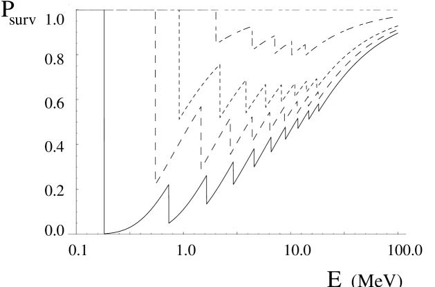
FIG. 1.: Survival probability of $\nu_{e}$ from the sun as a function of energy. The (solid, long dashed, short dashed, long-short dashed, long-short-short dashed) curves are for $\lambda=(0,1,2,5,10^{3})\cdot 10^{-3}\,{\rm eV}$. The purpose of this plot is only to illustrate the dependence of $P_{surv}$ on $\lambda$. The details of neutrino production and transport inside the sun and the energy resolution have not been taken into account. These will result in a smearing of the energy dependence shown in the figure.

FIG. 2.: $\Delta m^{2}_{41}$ in $\,{\rm eV}^{2}$ (the lower pair of curves) and the predicted LSND probability (eq. 59) $\chi_{e}^{2}\chi_{\mu}^{2}$ (the middle pair of curves) plotted against $\chi_{e}$. The solid (dotted) curves correspond to $\mu^{2}=1.0\;(0.2)\,{\rm eV}^{2}$. The uppermost horizontal lines are experimental LSND probabilities .02 and .003 corresponding to $\mu^{2}=1.0$ (solid) and $0.2\,{\rm eV}^{2}$ (dotted) respectively.

REFERENCES

- [1] S. Fukuda et al. [Super-Kamiokande Collaboration], Phys. Rev. Lett. 85 (2000) 3999 [hep-ex/0009001].
- [2] M. Apollonio et al. [CHOOZ Collaboration], Phys. Rev. D 61 (2000) 012001 [hep-ex/9906011].
- [3] S. Fukuda et al. [Super-Kamiokande Collaboration], hep-ex/0103033.
- [4] C. Athanassopoulos et al. [LSND Collaboration], Phys. Rev. Lett. 81 (1998) 1774 [nucl-ex/9709006].
- [5] K. Eitel [KARMEN Collaboration], Nucl. Phys. Proc. Suppl. 91 (2000) 191 [hep-ex/0008002].
- [6] K. Eitel, New Jour. Phys. 2 (2000) 1 [hep-ex/9909036].
- [7] S. Pakvasa, hep-ph/9905426; E. Ma and Probir Roy, Phys. Rev. Lett. 80 (1998) 4637; H. Nunokawa, hep-ph/0105027.
- [8] S. M. Bilenky, C. Guinti, W. Grimus and T. Schwetz, Phys. Rev. D 60 (1999) 073007; O. Peres and A. Yu. Smirnov, hep-ph/0011054.
- [9] V. Barger et al., Phys. Lett. B 489 (2000) 345.
- [10] W. Grimus and T. Schwetz, hep-ph/0102252
- [11] D. O. Caldwell and R. N. Mohapatra, Phys. Rev. D 48 (1993) 3259; J. Peltoniemi and J. W. F. Valle, Nucl. Phys. B 406 (1993) 409
- [12] M. C. Gonzalez-Garcia and C. Pena-Garay, Nucl. Phys. Proc. Suppl. 91 (2000) 80 [hep-ph/0009041].
- [13] E. J. Chun, A. S. Joshipura and A. Yu. Smirnov, Phys. Rev. D 54 (1996) 4654; Z. Berezhiani and R. N. Mohapatra, Phys. Rev. D 52 (1995) 6607; R. Foot and R. Volkas, Phys. Rev. D 52 (1995) 6595.
- [14] N. Arkani-Hamed, S. Dimopoulos and G. Dvali, Phys. Lett. B 429 (1998) 263 [hep-ph/9803315]. I. Antoniadis, N. Arkani-Hamed, S. Dimopoulos and G. Dvali, Phys. Lett. B 436 (1998) 257 [hep-ph/9804398]. N. Arkani-Hamed, S. Dimopoulos and G. Dvali, Phys. Rev. D 59 (1999) 086004 [hep-ph/9807344].
- [15] N. Arkani-Hamed, S. Dimopoulos, G. Dvali and J. March-Russell, hep-ph/9811448; K. R. Dienes, E. Dudas and T. Gherghetta, Nucl. Phys. B 557 (1999) 25.
- [16] A. Das and O. C. W. Kong, Phys. Lett. B 470 (1999) 149; A. Lukas and A. Romanino, hep-ph/0004130; R. N. Mohapatra, S. Nandi and A. Perez-Lorenzana, Phys. Lett. B 466 (1999) 175; R. N. Mohapatra and A. Perez-Lorenzana, Nucl. Phys. B 576 (2000) 466; A. Ioannission and J. W. F. Valle, Phys. Rev. D 62 (2000) 06600; J. Cosme et al., Phys. Rev. D 63 (2001) 113018 [hep-ph/0010192]. E. Ma, G. Rajasekaran and U. Sarkar, Phys. Lett. B 495 (2000) 363 [hep-ph/0006340].
- [17] G. Dvali and A. Y. Smirnov, Nucl. Phys. B 563 (1999) 63 [hep-ph/9904211].
- [18] R. Barbieri, P. Creminelli and A. Strumia, Nucl. Phys. B 585 (2000) 28; R. N. Mohapatra and A. Perez-Lorenzana, Nucl. Phys. B 593 (2001) 451.
- [19] A. Lukas, P. Ramond, A. Romanino and G. G. Ross, Phys. Lett. B 495 (2000) 136 [hep-ph/0008049].
- [20] K. Dienes and I. Sercevic, Phys. Lett. B 500 (2001) 133.
- [21] A. Ioannisian and J. W. Valle, Phys. Rev. D 63 (2001) 073002. D. Monderen, hep-ph/0104113. F. Ling, hep-ph/0105186.
- [22] A. Zee, Phys. Lett. B 93 (1980) 389 [Erratum-ibid. B 95 (1980) 461].
- [23] A. Lukas, P. Ramond, A. Romanino and G. G. Ross, JHEP 0104 (2001) 010 [hep-ph/0011295].
- [24] W. Grimus and L. Lavoura, JHEP 0011 (2000) 042 [hep-ph/0008179].
- [25] D. O. Caldwell, R. N. Mohapatra and S. J. Yellin, hep-ph/0010353, hep-ph/0101043; hep-ph/0102279.
- [26] A. Y. Smirnov and M. Tanimoto, Phys. Rev. D 55 (1997) 1665 [hep-ph/9604370].
- [27] P. H. Frampton and S. Glashow, hep-ph/9906375; C. Jarlskog et al., Phys. Lett. B 449 (1999) 240; A. S. Joshipura and S. D. Rindani, Phys. Lett. B 464 (1999) 239; D. Chang and A. Zee, Phys. Rev. D 61 (2000) 07130.
- [28] G. Barenboim, A. Dighe and S. Skadhauge, Preprints FERMILAB-Pub-01/078-T, MPI-PhT/2001-15, Lund-MPh-01/02.