1 Introduction

An outstanding task in heavy-flavor physics is to understand the strong interaction effects in exclusive weak decays of hadrons containing a $b$-quark. For many decay channels, such an understanding is a precondition for gaining information on the quark mixing matrix or on physics beyond the standard model. In addition, the dynamics of quarks, gluons, and hadrons in the presence of a large mass $m_{b}$ is interesting in QCD by its own right.

Introduced in [1], the concept of factorization has been one of the most successful tools in this respect, providing fair agreement between theory and data for many channels. In other cases, factorization in its most naive version fails when compared with experiment, and there have been several phenomenologically motivated improvements over its original form [2, 3].

There are several dynamical arguments why and where factorization should be valid. One is based on the large $N_{c}$ limit of QCD [4], whereas a different line of approach builds on the color transparency phenomenon [5]. More recently, the framework of QCD factorization has implemented the color transparency argument in the language of perturbation theory and power counting in $1/m_{b}$ [6, 7, 8].

In these approaches it is understood that there are corrections to naive factorization, which are suppressed in a small parameter such as $1/N_{c}$, or $\alpha_{s}$ and $\Lambda_{\mathrm{QCD}}/m_{b}$. A more quantitative understanding of their size is crucial in order to assess for which channels and to which precision the factorization concept can be applied. There are also scenarios where factorization in the sense of [1] does not appear as a limit when a small parameter vanishes, and where conceptually factorization breaking terms in the decay amplitude may be as large as the factorizing ones. An example is the perturbative hard scattering (PQCD) approach [9]. In view of such controversies, and given that present day theory can at best estimate the size of most nonfactorizing contributions, quantitative tests of factorization in the data are of great importance.

We propose here to study decay channels where the factorizing contributions to the amplitude are small or zero for symmetry reasons. In such a situation nonfactorizing contributions, which would otherwise be suppressed, have a chance to be clearly visible. The measurement of the corresponding decay rates can thus give rather direct information on their size, and the comparison of different channels may give indications on the relevant dynamical mechanisms.

Our suggestion is to choose decay channels whose flavor structure is such that a selected meson $X$ must be emitted from the weak current mediating the $b$-quark decay. Taking then a meson which has as very small decay constant, the factorizable contributions to the decay are suppressed. A second possibility is to consider mesons $X$ with spin $J\geq 2$. A tensor meson for instance cannot be produced from a decaying $W$ boson, which has spin 1, unless there are interactions involving the other hadrons in the decay process. We will find a variety of decay channels where these ideas can be realized, which will allow us to address different issues related to factorization and its breaking.

The organization of this paper is as follows. In Sect. 2 we review the basics of factorization which will be essential for our arguments. We select the mesons for which factorizing contributions in decays are suppressed in Sect. 3. In the following section we identify which flavor structure a decay must have in order for this suppression to apply, and take a closer look at specific issues in the different channels. Sect. 5 discusses how suppression can be circumvented by different nonfactorizing mechanisms. Some of these can be treated within QCD factorization and will be investigated in Sect. 6. We estimate branching ratios of suppressed decays into a heavy and a light meson in the subsequent section, before concluding in Sect. 8. Some numerical estimates concerning meson distribution amplitudes, which we need in our paper, are given in an Appendix.

2 Matrix elements for hadronic two-body decays

We start by briefly recalling the low-energy effective Hamiltonian and some basics of the factorization approach. Hadronic two-body $b$-decays are described by the effective weak Hamiltonian

$${\cal{H}}_{\mathrm{eff}}=\frac{G_{F}}{\sqrt{2}}\left[\,\sum_{j,k=u,c}V_{jb}^{\phantom{*}}V^{*}_{kd}\,\Big{(}C_{1}^{\phantom{j}}O_{1}^{jk}+C_{2}^{\phantom{j}}O_{2}^{jk}\Big{)}-V_{tb}^{\phantom{*}}V^{*}_{td}\sum_{i}C_{i}O_{i}\,\right]+\{d\rightarrow s\}+\mathrm{h.c.}\,,$$ (1)

where $V$ denotes the CKM matrix. The operators $O_{1,2}^{jk}$ result from tree level $W$ exchange and in the case $i=k=u$ read

$$O_{1}^{uu} = \bar{u}_{\alpha}\gamma^{\mu}(1-\gamma_{5})b_{\alpha}\>\bar{d}_{\beta}\gamma_{\mu}(1-\gamma_{5})u_{\beta},$$

$$O_{2}^{uu} = \bar{u}_{\alpha}\gamma^{\mu}(1-\gamma_{5})b_{\beta}\>\bar{d}_{\beta}\gamma_{\mu}(1-\gamma_{5})u_{\alpha}.$$ (2)

Here $\alpha$ and $\beta$ are color indices, and it is understood that all fields are taken at space-time argument zero. The remaining operators in ${\cal{H}}_{\mathrm{eff}}$ are so-called penguins. For a detailed discussion of the operators $O_{i}$ and the Wilson coefficients $C_{i}$ we refer to [10].

In naive factorization, the matrix element $\langle YX|\,{\cal{H}}_{\mathrm{eff}}\,|B\rangle$ is written as a product of matrix elements of quark currents between $B$ and $Y$, and between the vacuum and $X$. Only the color-singlet piece of each current is retained, while the color-octet piece is neglected. This leads to replacing ${\cal{H}}_{\mathrm{eff}}$ by the effective transition operator ${\cal T}$, whose tree level operators read

$${\cal T}^{(1,2)} = \frac{G_{F}}{\sqrt{2}}\,V^{\phantom{*}}_{ub}V_{ud}^{*}\,\Big{[}\,a_{1}\;\bar{u}\gamma^{\mu}(1-\gamma_{5})b\otimes\bar{d}\gamma_{\mu}(1-\gamma_{5})u$$ (3)

$$\hskip 40.00006pt{}+a_{2}\;\bar{d}\gamma^{\mu}(1-\gamma_{5})b\otimes\bar{u}\gamma_{\mu}(1-\gamma_{5})u\,\Big{]}$$

for $i=k=u$. Here the notation $\otimes$ indicates that the matrix elements are to be taken in factorized form as described above. The new coefficients $a_{1}=C_{1}+C_{2}/3$ and $a_{2}=C_{2}+C_{1}/3$ have been obtained from projecting on color-singlet currents, and are commonly referred to as color allowed and color suppressed, respectively. Numerically, $a_{1}$ is close to 1 and $a_{2}$ of order 0.1 at a renormalization scale $\mu=m_{b}$. Notice that the Fierz transform performed in the second term of Eq. (3) has left the $(V-A)\times(V-A)$ structure invariant, where $V$ and $A$ respectively denote the vector and axial vector current. The situation is analogous for those penguin operators which again involve $(V-A)\times(V-A)$ currents, for explicit formulae see e.g. [8].

Important for us will be the strong penguins with $(V-A)\times(V+A)$ structure (the electroweak ones with similar Dirac structure are numerically less important in the Standard Model). They are

$$O_{5} = \bar{d}_{\alpha}\gamma^{\mu}(1-\gamma_{5})b_{\alpha}\>\sum_{q}\bar{q}_{\beta}\gamma_{\mu}(1+\gamma_{5})q_{\beta},$$

$$O_{6} = \bar{d}_{\alpha}\gamma^{\mu}(1-\gamma_{5})b_{\beta}\>\sum_{q}\bar{q}_{\beta}\gamma_{\mu}(1+\gamma_{5})q_{\alpha},$$ (4)

with a sum over $q=u,d,s,c,b$, and in naive factorization lead to

$${\cal T}^{(5,6)} = -\frac{G_{F}}{\sqrt{2}}\,V^{\phantom{*}}_{tb}V_{td}^{*}\,\Big{[}\,a_{5}\;\sum_{q}\bar{d}\gamma^{\mu}(1-\gamma_{5})b\otimes\bar{q}\gamma_{\mu}(1+\gamma_{5})q$$ (5)

$$\hskip 45.00006pt{}+a_{6}\;\sum_{q}\,(-2)\,\bar{q}(1-\gamma_{5})b\otimes\bar{d}(1+\gamma_{5})q\;\Big{]}.$$

The structure $(P-S)\times(P+S)$ involving the scalar and pseudoscalar currents $S$ and $P$ has emerged from the Fierz transform in the term with $a_{6}=C_{6}+C_{5}/3$, whose value is about $-0.03$ at $\mu=m_{b}$. The corresponding operator provides one possibility to circumvent the suppression mechanisms we will discuss shortly, and we will often refer to it as scalar penguin.

3 Meson candidate selection

Let us now specify our mechanisms to suppress decay amplitudes in naive factorization and see to which final states they apply.

3.1 Suppression mechanisms

There are several reasons why the coupling of a meson to the local currents of the effective weak Hamiltonian can be suppressed. Clearly, a meson with spin $J=2$ or larger has no matrix element with either of the currents $S$, $P$, $V$, $A$, and in naive factorization cannot be produced as a meson ejected by the effective weak current. From Table 1 we see that examples for such mesons are the $a_{2}$, $\pi_{2}$, $\rho_{3}$, and $K^{*}_{2}$ in the light quark sector. Heavy tensor mesons are the $D_{2}^{*}$ and $D_{sJ}$, and there is a tensor charmonium state, $\chi_{2c}$.

$X$	$a_{0}$	$b_{1}$	$\pi$	$a_{2}$	$a_{0}$	$\pi_{2}$	$\rho_{3}$	$\pi$	$a_{4}$	$\chi_{c0}$	$\chi_{c2}$
$m_{X}$ [MeV]	985	1230	1300	1318	1474	1670	1691	1801	2014	3415	3556
$J^{PC}$	$0^{++}$	$1^{+-}$	$0^{-+}$	$2^{++}$	$0^{++}$	$2^{-+}$	$3^{--}$	$0^{-+}$	$4^{++}$	$0^{++}$	$2^{++}$

$X$	$K_{0}^{*}$	$K_{2}^{*}$	$K_{2}$	$K_{3}^{*}$	$K_{2}$	$K_{4}^{*}$	$D_{2}^{*}$	$D_{sJ}$
$m_{X}$ [MeV]	1412	1426	1773	1776	1816	2045	2459	2573
$J^{P}$	$0^{+}$	$2^{+}$	$2^{-}$	$3^{-}$	$2^{-}$	$4^{+}$	$2^{+}$	$(2^{+})$

Table 1: Mesons for which one of the suppression mechanisms discussed in Sect. 3.1 is relevant. Masses are taken from the Review of Particle Data [11]. We do not list those mesons that are omitted in the meson summary table. The spin-parity assignment for the $D_{sJ}(2537)$ is not certain yet.

Let us now turn to mesons with $J=0,1$ whose production from the weak current in naive factorization is forbidden or suppressed because their coupling to $V$ and $A$ is zero or small. We define the decay constants of the negatively charged mesons with isospin $I=1$ as

$$\langle{S(q)}|\,{\bar{d}(0)\,\gamma^{\mu}\,u(0)}\,|0\rangle = -if_{S}\,q^{\mu},$$ (6)

$$\langle{P(q)}|\,{\bar{d}(0)\,\gamma^{\mu}\gamma_{5}\,u(0)}\,|0\rangle = -if_{P}\,q^{\mu},$$ (7)

$$\langle{V(q,\epsilon)}|\,{\bar{d}(0)\,\gamma^{\mu}\,u(0)}\,|0\rangle = -if_{V}m_{V}\epsilon^{\mu},$$ (8)

$$\langle{A(q,\epsilon))}|\,{\bar{d}(0)\,\gamma^{\mu}\gamma_{5}\,u(0)}\,|0\rangle = -if_{A}m_{A}\epsilon^{\mu},$$ (9)

for scalar, pseudoscalar, vector, and axial mesons, respectively. Here $q^{\mu}$ denotes the meson momentum and, if applicable, $\epsilon^{\mu}$ its polarization vector. The choice of vector or axial quark current on the right-hand sides of these definitions is dictated by the parity of the meson. For the corresponding neutral mesons, the flavor structure of the current is $(\bar{u}u-\bar{d}d)/\sqrt{2}$ instead of $\bar{d}u$, and for mesons with different quark content one has to take $\bar{s}d$, $\bar{s}u$, $\bar{c}c$, etc.

Because of charge conjugation invariance, the decay constants for the neutral $a_{0}$ and $b_{1}$ mesons and for the $\chi_{0c}$ must be zero. In the isospin limit, the decay constants of the charged $a_{0}$ and $b_{1}$ must thus vanish, too, so that $f_{a0}$ and $f_{b1}$ defined in Eqs. (6), (9) are small, of order $m_{d}-m_{u}$. For the $a_{0}$ mesons, this can explicitly be seen by taking the divergence of Eq. (6), which by virtue of the equations of motion gives

$$m_{a_{0}}^{2}\,f_{a_{0}}^{\phantom{a_{0}}} = i(m_{d}-m_{u})\,\langle{a_{0}}|\,{\bar{d}(0)u(0)}\,|0\rangle.$$ (10)

For the charged $K^{*}_{0}$ the analogous relation reads

$$m_{K^{*}_{0}}^{2}\,f_{K^{*}_{0}}^{\phantom{K^{*}_{0}}} = i(m_{s}-m_{u})\,\langle{K^{*}_{0}}|\,{\bar{s}(0)u(0)}\,|0\rangle,$$ (11)

which becomes zero in the flavor SU(3) limit and indicates that $f_{K^{*}_{0}}$ should be suppressed.

It is instructive to compare Eqs. (10) and (11) with their analogs for the pseudoscalars,

$$m_{\pi}^{2}\,f_{\pi}^{\phantom{\pi}} = i(m_{d}+m_{u})\,\langle{\pi}|\,{\bar{d}(0)\gamma_{5}u(0)}\,|0\rangle,$$ (12)

$$m_{K}^{2}\,f_{K}^{\phantom{K}} = i(m_{s}+m_{u})\,\langle{K}|\,{\bar{s}(0)\gamma_{5}u(0)}\,|0\rangle.$$ (13)

Because the axial current is not conserved, these decay constants do not vanish in the isospin or SU(3) limit. Moreover, they do not vanish in the chiral limit, $m_{u}=m_{d}=m_{s}=0$, for the light pion and kaon, since these mesons are Goldstone bosons and become massless in the same limit. Numerically, $f_{\pi}$ and $f_{K}$ are in fact not small and of the same order of magnitude as for instance $f_{\rho}$ and $f_{K^{*}}$. The decay constant for the heavy $\pi(1300)$, however, does become zero in the chiral limit, and its actual value is small due to chiral suppression.

We remark that the spin-zero mesons whose coupling to the $V$ and $A$ currents is small or zero for one of the above reasons can still couple to the $S$ or $P$ currents appearing in penguin operators of the effective Hamiltonian, as discussed in Sect. 2. This does however not hold for the $b_{1}$, which has no matrix elements with $S$ or $P$.

3.2 Decay constants

The decay constants of the $a_{0}(980)$, $a_{0}(1450)$, $K^{*}_{0}$, $\pi(1300)$, and the $b_{1}$ are poorly known at present. Using finite energy sum rules, Maltman [12] obtained

$$f_{a0(980)}=1.1\mbox{~{}MeV},\hskip 20.00003ptf_{a0(1450)}=0.7\mbox{~{}MeV},\hskip 20.00003ptf_{K^{*}_{0}}=42\mbox{~{}MeV},$$ (14)

consistent with the ranges estimated by Narison [13]

$$f_{a0(980)}=0.7\mbox{~{}to~{}}2.5\mbox{~{}MeV},\hskip 20.00003ptf_{K^{*}_{0}}=33\mbox{~{}to~{}}46\mbox{~{}MeV}.$$ (15)

For the heavy pion, the theoretical estimates in [14] provide a range

$$f_{\pi(1300)}=0.5\mbox{~{}to~{}}7.2\mbox{~{}MeV}.$$ (16)

Comparing these values to

$$f_{\pi}=131\mbox{~{}MeV},\hskip 20.00003ptf_{K}=160\mbox{~{}MeV},$$ (17)

we find that the suppression patterns discussed in the previous subsection are indeed seen numerically, with the decay constants for the $a_{0}$ mesons smaller than those for $\pi(1300)$ because of the relative signs between the quark masses in Eqs. (10) and (12). We also see that $f_{K^{*}_{0}}$ is suppressed relative to $f_{K}$, but not as strongly as $f_{a_{0}}$ compared with $f_{\pi}$, because SU(3) symmetry breaking is rather strong for the quark masses. Here we have implicitly assumed that the (pseudo)scalar matrix elements on the right-hand sides of Eqs. (10) to (13) are not anomalously small or large. Indeed, taking from [15] 

$$m_{u}=4.8\mbox{~{}MeV},\hskip 20.00003ptm_{d}=8.7\mbox{~{}MeV},\hskip 20.00003ptm_{s}=164\mbox{~{}MeV}$$ (18)

for the $\overline{\mbox{MS}}$ quark masses at $\mu=1$ GeV, we find with the values (16) and (17)

$$i\,\langle{\pi}|\,{\bar{d}\gamma_{5}u}\,|0\rangle \approx 0.19\mbox{~{}GeV}^{2},$$

$$i\,\langle{\pi(1300)}|\,{\bar{d}\gamma_{5}u}\,|0\rangle \approx 0.06\mbox{~{}to~{}}0.90\mbox{~{}GeV}^{2},$$

$$i\,\langle{K}|\,{\bar{s}\gamma_{5}u}\,|0\rangle \approx 0.23\mbox{~{}GeV}^{2},$$ (19)

and with (14) and (15)

$$i\,\langle{a_{0}(980)}|\,{\bar{d}u}\,|0\rangle \approx 0.17\mbox{~{}to~{}}0.62\mbox{~{}GeV}^{2},$$

$$i\,\langle{a_{0}(1450)}|\,{\bar{d}u}\,|0\rangle \approx 0.39\mbox{~{}GeV}^{2},$$

$$i\,\langle{K^{*}_{0}(1430)}|\,{\bar{s}u}\,|0\rangle \approx 0.42\mbox{~{}to~{}}0.58\mbox{~{}GeV}^{2}.$$ (20)

Despite a certain spread these values are remarkably close to each other, given that the corresponding squared meson masses vary by more than two orders of magnitude. We note that Chernyak [16] has recently estimated $f_{K^{*}_{0}}=(70\pm 10)$ MeV. We consider this to be rather high as it is far away from the range (15) obtained in other studies. Also, the corresponding value for $\langle{K^{*}_{0}(1430)}|\,{\bar{s}u}\,|0\rangle$ would correspond to a quite strong SU(3) breaking for the scalar matrix elements.

We wish to emphasize at this point that the decay constants for the $a_{0}(980)$, $a_{0}(1450)$, $K^{*}_{0}$, $\pi(1300)$, and the $b_{1}$ can be measured very cleanly in $\tau$ decays. In fact, from the bound on the branching ratio ${\cal{B}}(\tau\to\pi(1300)\nu_{\tau})<1\cdot 10^{-4}$ in [11] we infer $f_{\pi(1300)}<8.4$ MeV, which is not far from the upper end of the theory estimates (16). The decay constants in Eq. (14) correspond to branching ratios of

$${\cal{B}}(\tau\to a_{0}(980)\,\nu_{\tau}) \simeq 3.8\cdot 10^{-6},$$

$${\cal{B}}(\tau\to a_{0}(1450)\,\nu_{\tau}) \simeq 3.7\cdot 10^{-7},$$

$${\cal{B}}(\tau\to K^{*}_{0}(1430)\,\nu_{\tau}) \simeq 7.7\cdot 10^{-5}.$$ (21)

These estimates are rather encouraging, given that at the $B$ factories one expects to have about $3\cdot 10^{7}$ $\tau$ pairs with 30 fb^-1 [17], and that the potential of $\tau$-charm factories would be even higher. A measurement of the decay constants for the above mesons would greatly reduce the uncertainties in the predictions we will give in Sect. 7. It could also provide valuable information on the nature in particular of the $a_{0}(980)$ and $a_{0}(1450)$, only one of which can be a member of the conventional $q\bar{q}$ meson nonett.

3.3 Kinematics

The color transparency argument [5] for factorization of decays $B\to YX$ requires the meson $X$ emitted from the weak current to be fast. More quantitatively, its time dilation factor $E_{X}/m_{X}$ should be large, where $E_{X}=(m_{B}^{2}-m_{Y}^{2}+m_{X}^{2})/(2m_{B})$ is the energy of $X$ in the $B$ meson rest frame. We show the values of $E_{X}/m_{X}$ for $Y=D$ and $Y=\pi$ in Fig. 1. The corresponding curves for $B\to D^{*}X$ and $B_{s}\to D_{s}^{(*)}X$ are very close to the one for $B\to DX$, and the ones for $B\to\rho X$, $B_{s}\to KX$, and $B_{s}\to K^{*}(892)\,X$ are practically the same as for $B\to\pi X$. Only if $X$ is a pion does one have a very large $E_{X}/m_{X}$, namely $E_{\pi}/m_{\pi}=16.5$ for $B\to D\pi$ and $E_{\pi}/m_{\pi}=19$ for $B\to\pi\pi$. For $m_{X}$ above 1 GeV, relevant for the mesons in Table 1, this ratio decreases rather gently from moderate values down to little above 1. Even so, the mass range of our candidate mesons seems sufficiently large so that a study of the corresponding decay channels could provide valuable clues to whether corrections to factorization significantly depend on $E_{X}/m_{X}$, or more generally, on the mass $m_{X}$. We remark in passing that even the lowest value of $E_{X}/m_{X}$ in Fig. 1 corresponds to a velocity $\beta_{X}=0.5$ and a recoil momentum of $p_{X}=1.5$ GeV in the $B$ rest frame, indicating that $X$ is still relativistic.

Figure 1: Values of $E_{X}/m_{X}$ as a function of $m_{X}$ for the decays $B\to DX$ (lower curve) and $B\to\pi X$ (upper curve).

3.4 Resonance decays and the continuum

Clearly, the measurement of rare $B$ decays involving higher mass resonances presents an experimental challenge. An experimental analysis will be easier if the meson $X$ in question has a decay channel with sizeable branching fraction that is not also accessible to mesons with nearby mass whose production is not suppressed. To give some examples, the decays of $a_{0}(980)$, $a_{2}(1320)$, and $a_{0}(1450)$ into $\pi\eta$ appear rather clean in this respect, as do the modes $b_{1}(1235)\to\omega\pi$ and $\pi_{2}(1670)\to f_{2}(1270)\pi$. On the other hand, the decays of $a_{2}(1320)$, $\pi(1300)$, and $\pi_{2}(1670)$ into $\rho\pi$ are more problematic because of background from the rather broad $a_{1}(1260)$. The same holds true for the decays of the $K_{0}^{*}(1430)$ and $K_{2}^{*}(1430)$ into $K\pi$ because of background from the $K^{*}(1410)$. In such cases a partial wave analysis of the decay products will probably be necessary in order to constrain the decays into the mesons with spin $J=0$ or $J=2$.

We emphasize at this point that mesons $X$ with a rather large decay width do not present as serious a problem in our context as in other studies. The physical arguments leading to a suppression of their production within the factorization mechanism (as the arguments for factorization itself) do in fact not depend on $X$ being a narrow resonance. Our arguments in Sect. 3.1 were at the level of current matrix elements and go through in complete analogy if, for instance, the $|\pi(1300)\rangle$ state in Eq. (12) is replaced with $|\rho\pi\rangle$ in appropriate partial waves that have definite quantum numbers $J^{P}=0^{-}$. Moreover, the main idea here is to use the branching ratios of suppressed decays as quantitative estimates for the size of corrections to factorization, and to study their pattern by comparing different decay channels. An uncertainty on the branching ratio of $B\to YX$ due to the line shape of $X$ is therefore less severe as in channels which are allowed by factorization, and where factorization tests need branching ratios to a much higher precision.

One could in fact also perform the studies we propose here not with particular meson resonances but with continuum states, similarly to a recent test of factorization by Ligeti et al. [18]. Our main reason to concentrate on resonances $X$ here is that, by definition, their production should be enhanced with respect to continuum states with the same quantum numbers, which is important since we are looking for decays with small branching ratios from the start.

4 Decay mode selection

We are looking for exclusive decays $B\to YX$, where the meson $X$ must be emitted from the weak decay vertex and cannot pick up the spectator quark. Only then will the factorizing contribution to the decay be suppressed for mesons $X$ with small or vanishing decay constant or with spin $J\geq 2$. This puts requirements on the flavor structure of the decay, which we now discuss. One may avoid these requirements by studying decays where both final state mesons are taken from Table 1, such as $\bar{B}^{0}\to b_{1}^{+}b_{1}^{-}$ or $\bar{B}^{0}\to\pi_{2}^{+}a_{2}^{-}$. For one of the mesons the appropriate suppression mechanism will then always be at work.

For definiteness we consider in the following the case where the $B$ meson contains a $b$ and not a $\bar{b}$. One requirement now is that the flavors of the spectator antiquark and of the antiquark emitted from the $b$ decay must not be the same, otherwise $X$ can pick up either of them. We thus cannot use decays such as $B^{-}\to D^{0}a_{0}^{-}$, whose flavor structure reads $\bar{u}b\to\bar{u}(c\bar{u}d)$, where the brackets indicate the quarks originating from the electroweak vertex.

A second requirement is due to imperfect knowledge of the initial state. Whereas the decay $\bar{B}^{0}\to D^{+}a_{0}^{-}$ with flavor structure $\bar{d}b\to\bar{d}(c\bar{u}d)$ satisfies our requirement, the same final state can be reached in the decay of a $B^{0}$, where the $a_{0}^{-}$ contains the spectator. The corresponding diagrams are shown in Fig. 2. This $C\!P$ conjugated background can in principle be removed by flavor tagging, which puts of course stronger demands on the experiment. In the example just given, the amplitude from $B^{0}$ decay is suppressed by $\lambda^{2}$ relative to the direct decay, where $\lambda\approx 0.22$ is the Wolfenstein parameter in the CKM matrix. We will give a more quantitative estimate of this background in Sect. 7.1. In other cases however, e.g. for $\bar{B}_{s}\to D_{s}^{+}K_{0}^{*-}$ versus $B_{s}\to D_{s}^{+}K_{0}^{*-}$, both signal and background amplitudes are of order $\lambda^{3}$. We will not consider such modes in the following, and list in Tables 2 and 3 the flavor structure of decays satisfying the following conditions:

1. It is ensured that the meson selected from Table 1 cannot pick up the spectator antiquark in the $B$ meson.

2. A $C\!P$ conjugated background that violates condition 1 either does not exist or is CKM suppressed. It turns out that the only case we retain that has such a background is the one mentioned above, listed in the first row of Table 2.

Let us now consider the different decay categories separately.

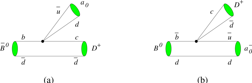
Figure 2: Tree level diagrams for (a) $\bar{B}^{0}\to D^{+}a_{0}^{-}$ and (b) $B^{0}\to D^{+}a_{0}^{-}$.

example decay	factorizing contribution			annihilation
	quark level	tree	peng.	topology	tree	peng.
$\bar{B}^{0}\to D^{+}a_{0}^{-}$	$\bar{d}b\to\bar{d}(c\bar{u}d)$	$\lambda^{2}$		a	$\lambda^{2}$
$\phantom{\bar{B}^{0}}\to D^{+}K_{0}^{*-}$	$\phantom{\bar{d}b}\to\bar{d}(c\bar{u}s)$	$\lambda^{3}$
$\bar{B}_{s}\to D_{s}^{+}a_{0}^{-}$	$\bar{s}b\to\bar{s}(c\bar{u}d)$	$\lambda^{2}$
$\bar{B}^{0}\to\pi^{+}D_{sJ}^{-}$	$\bar{d}b\to\bar{d}(u\bar{c}s)$	$\lambda^{3}$
$B^{-}\to\pi^{0}D_{2}^{*-}$	$\bar{u}b\to\bar{u}(u\bar{c}d)$	$\lambda^{4}$		a	$\lambda^{4}$
$\phantom{B^{-}}\to\eta D_{2}^{*-}$	$\phantom{\bar{u}b}\to\bar{u}(u\bar{c}d)$	$\lambda^{4}$		a, c	$\lambda^{4}$
$\phantom{B^{-}}\to\pi^{0}D_{sJ}^{-}$	$\phantom{\bar{u}b}\to\bar{u}(u\bar{c}s)$	$\lambda^{3}$
$\phantom{B^{-}}\to\eta D_{sJ}^{-}$	$\phantom{\bar{u}b}\to\bar{u}(u\bar{c}s)$	$\lambda^{3}$		a, c	$\lambda^{3}$
$\bar{B}_{s}\to K^{+}D_{2}^{*-}$	$\bar{s}b\to\bar{s}(u\bar{c}d)$	$\lambda^{4}$
$\bar{B}^{0}\to D^{+}D_{sJ}^{-}$	$\bar{d}b\to\bar{d}(c\bar{c}s)$	$\lambda^{2}$	$\lambda^{2}$	a		$\lambda^{2}$
$B^{-}\to D^{0}D_{2}^{*-}$	$\bar{u}b\to\bar{u}(c\bar{c}d)$	$\lambda^{3}$	$\lambda^{3}$	a	$\lambda^{3}$	$\lambda^{3}$
$\phantom{B^{-}}\to D^{0}D_{sJ}^{-}$	$\phantom{\bar{u}b}\to\bar{u}(c\bar{c}s)$	$\lambda^{2}$	$\lambda^{2}$	a	$\lambda^{4}$	$\lambda^{2}$
$\bar{B}_{s}\to D_{s}^{+}D_{2}^{*-}$	$\bar{s}b\to\bar{s}(c\bar{c}d)$	$\lambda^{3}$	$\lambda^{3}$	a		$\lambda^{3}$
$\bar{B}^{0}\to\pi^{+}K_{2}^{*-}$	$\bar{d}b\to\bar{d}(u\bar{u}s)$	$\lambda^{4}$	$\lambda^{2}$	a		$\lambda^{2}$
$B^{-}\to\pi^{-}\bar{K}_{2}^{*0}$	$\bar{u}b\to\bar{u}(d\bar{d}s)$		$\lambda^{2}$	a	$\lambda^{4}$	$\lambda^{2}$
$\phantom{B^{-}}\to K^{-}K_{2}^{*0}$	$\phantom{\bar{u}b}\to\bar{u}(s\bar{s}d)$		$\lambda^{3}$	a	$\lambda^{3}$	$\lambda^{3}$
$\bar{B}_{s}\to K^{+}a_{2}^{-}$	$\bar{s}b\to\bar{s}(u\bar{u}d)$	$\lambda^{3}$	$\lambda^{3}$	a		$\lambda^{3}$

Table 2: Color allowed decay modes $B\to YX$ satisfying the criteria specified in the text. $X$ is the meson emitted from the weak decay vertex. Any meson can be replaced by another with the same flavor structure and isospin, e.g, $D$ by $D^{*}$, $\pi$ by $\rho$, and the meson $X$ by an appropriate candidate from Table 1. The second column gives the quark composition of the final state, with the quarks originating from the $b$ decay enclosed in brackets. In the third and fourth columns we give the power of the Wolfenstein parameter $\lambda$ in the decay amplitude for tree level $W$ exchange and penguin operators, respectively. Annihilation contributions are listed with their topology as shown in Fig. 5 and the power of the Wolfenstein parameter for tree level and penguin operators.

example decay	factorizing contribution			annihilation
	quark level	tree	peng.	topology	tree	peng.
$\bar{B}^{0}\to\pi^{0}D_{2}^{*0}$	$\bar{d}b\to\bar{d}(d\bar{u}c)$	$\lambda^{2}$		a	$\lambda^{2}$
$\phantom{\bar{B}^{0}}\to\eta\,D_{2}^{*0}$	$\phantom{\bar{d}b}\to\bar{d}(d\bar{u}c)$	$\lambda^{2}$		a, c	$\lambda^{2}$
$B^{-}\to K^{-}D_{2}^{*0}$	$\bar{u}b\to\bar{u}(s\bar{u}c)$	$\lambda^{3}$
$\bar{B}_{s}\to K^{0}D_{2}^{*0}$	$\bar{s}b\to\bar{s}(d\bar{u}c)$	$\lambda^{2}$
$\phantom{\bar{B}_{s}}\to\eta\,D_{2}^{*0}$	$\phantom{\bar{s}b}\to\bar{s}(s\bar{u}c)$	$\lambda^{3}$		a, c	$\lambda^{3}$
$\bar{B}^{0}\to\bar{K}^{0}\chi_{c0}$	$\bar{d}b\to\bar{d}(s\bar{c}c)$	$\lambda^{2}$	$\lambda^{2}$	b		$\lambda^{2}$
$\phantom{\bar{B}^{0}}\to\pi^{0}\chi_{c0}$	$\phantom{\bar{d}b}\to\bar{d}(d\bar{c}c)$	$\lambda^{3}$	$\lambda^{3}$	b	$\lambda^{3}$	$\lambda^{3}$
$\phantom{\bar{B}^{0}}\to\eta\,\chi_{c0}$	$\phantom{\bar{d}b}\to\bar{d}(d\bar{c}c)$	$\lambda^{3}$	$\lambda^{3}$	b, c	$\lambda^{3}$	$\lambda^{3}$
$B^{-}\to K^{-}\chi_{c0}$	$\bar{u}b\to\bar{u}(s\bar{c}c)$	$\lambda^{2}$	$\lambda^{2}$	b	$\lambda^{4}$	$\lambda^{2}$
$\phantom{B^{-}}\to\pi^{-}\chi_{c0}$	$\phantom{\bar{u}b}\to\bar{u}(d\bar{c}c)$	$\lambda^{3}$	$\lambda^{3}$	b	$\lambda^{3}$	$\lambda^{3}$
$\bar{B}_{s}\to\eta\,\chi_{c0}$	$\bar{s}b\to\bar{s}(s\bar{c}c)$	$\lambda^{2}$	$\lambda^{2}$	b, c	$\lambda^{2}$	$\lambda^{2}$
$\phantom{\bar{B}_{s}}\to K^{0}\chi_{c0}$	$\phantom{\bar{s}b}\to\bar{s}(d\bar{c}c)$	$\lambda^{3}$	$\lambda^{3}$	b		$\lambda^{3}$
$\bar{B}_{s}\to K^{0}\,a_{2}^{0}$	$\bar{s}b\to\bar{s}(d\bar{u}u)$	$\lambda^{3}$	$\lambda^{3}$	a		$\lambda^{3}$
$\phantom{\bar{B}_{s}}\to\eta\;a_{2}^{0}$	$\phantom{\bar{s}b}\to\bar{s}(s\bar{u}u)$	$\lambda^{4}$	$\lambda^{2}$	a, c	$\lambda^{4}$	$\lambda^{2}$

Table 3: As Table 2 but for decays where the tree level contribution is color suppressed. We remark that the decay $\bar{B}_{s}\to K^{0}\,a_{2}^{0}$ has a color allowed penguin contribution.

4.1 Decays with one or two heavy mesons

Decays into heavy-light final states with open charm are the simplest from the point of view of their electroweak structure, since only the $W$ exchange operators $O_{1}$ and $O_{2}$ of the effective Hamiltonian contribute. For color allowed decays $B\to DX$ with $X=\pi,\rho,a_{1}$, naive factorization is in rather good agreement with data [2, 19].

For color allowed decays where the heavy meson is the emission particle, the color transparency argument does not hold, but arguments based on the large $N_{c}$ limit do. Relevant meson candidates here are the $D_{2}^{*}$ and the $D_{sJ}$. Comparing the size of nonfactorizing contributions for the two types of channels with the suppression mechanisms discussed here might thus shed light on the question which type of mechanism is more relevant to ensure factorization. One may also use decays into two charmed mesons to address the same question. We remark in this context that in recent study, Luo and Rosner found factorization to work reasonably well for $\bar{B}^{0}\to D^{(*)+}D_{s}^{(*)-}$ within present errors [19].

Notice that for color suppressed channels such as $\bar{B}^{0}\to\pi^{0}D_{2}^{*0}$ naive factorization is neither backed up by color transparency nor by $1/N_{c}$ arguments. The decays into a $D_{2}^{*0}$ in Table 3 will thus show whether the factorization concept still applies here.

Let us finally consider $B$ decays into charmonium. Naive factorization has notorious problems with these channels [2], compounded by the fact that the coefficient $a_{2}$ is extremely dependent on the factorization scale $\mu$. A comparison of the decays involving a $\chi_{c0}$ or $\chi_{c2}$ and the corresponding ones with $J/\psi$ or $\chi_{c1}$ may thus shed light on the relative importance of factorizable and nonfactorizable contributions.

4.2 Penguins and decays into two light mesons

Decays into two light mesons present some specifics due to the presence of penguin operators. First, we have no meson candidates with isospin $I=0$, which are a superposition of quark states $u\bar{u}$, $d\bar{d}$, $s\bar{s}$. Penguin transitions lead to all three of them, and one will always violate our condition that the spectator and the emitted antiquark must have different flavors. Second, as remarked at the end of Sect. 3.1, suppression mechanisms based on the smallness of the decay constant $f_{X}$ are not effective if scalar penguins occur in the factorization ansatz. Only spin suppression, and the isospin suppression for the $b_{1}$, are still at work then.

It is nevertheless instructive to look at the relative importance of the $S$ and $P$ operators in decays involving scalars or pseudoscalars. In the decays $\bar{B}^{0}\to a_{0}^{+}\,a_{0}^{-}$ or $\bar{B}^{0}\to\pi^{+}(1300)\pi^{-}(1300)$ the scalar penguins come with huge enhancement factors in the amplitudes

$$r^{a_{0}}=\frac{2m_{a_{0}}^{2}}{m_{b}\,(m_{d}-m_{u})},\hskip 20.00003ptr^{\pi}=\frac{2m_{\pi}^{2}}{m_{b}\,(m_{d}+m_{u})}.$$ (22)

Numerically, $r^{\pi(1300)}=85$, $r^{a_{0}(980)}=170$, and $r^{a_{0}(1450)}=380$, to be compared with $r^{\pi}=1$ for the light pion, where we have evolved the light quark masses (18) up to $\mu=m_{b}=4.4$ GeV. The strong scalar penguin can hence compete with the current-current operators, even though its coefficient $a_{6}$ introduced in Sect. 2 is only of order of several $10^{-2}$.

Using Eqs. (10), (12), (22), we can express the products $f_{X}r^{X}$ in terms of the (pseudo)scalar matrix elements (19) and (20), and observe that

$$f_{a_{0}}r^{a_{0}}\approx f_{\pi(1300)}r^{\pi(1300)}\approx f_{\pi}r^{\pi},$$ (23)

i.e., they are all roughly of the same size. Since $\bar{B}^{0}\to\pi^{+}\pi^{-}$ is driven by the color allowed tree level coefficient $a_{1}$, naive factorization predicts the decay rate for $\bar{B}^{0}\to a_{0}^{+}\,a_{0}^{-}$ to be small compared with the one for $\bar{B}^{0}\to\pi^{+}\pi^{-}$. Namely, the ratio of their amplitudes is controlled by the small parameters $f_{a_{0}}/f_{\pi}$ and

$$\frac{a_{6}}{a_{1}}\,\frac{f_{a_{0}}r^{a_{0}}}{f_{\pi}}=\frac{a_{6}}{a_{1}}\,r^{\pi}\,\frac{\langle{a_{0}}|\,{\bar{d}u}\,|0\rangle}{\langle{\pi}|\,{\bar{d}\gamma_{5}\,u}\,|0\rangle},$$ (24)

corresponding to the tree level and scalar penguin contribution to $\bar{B}^{0}\to a_{0}^{+}\,a_{0}^{-}$, respectively. Analogous estimates can be given for $\bar{B}^{0}\to\pi^{+}(1300)\,\pi^{-}(1300)$, and also for $\bar{B}_{s}$ decays into $K^{+}a_{0}^{-}$ and $K^{+}\pi^{-}(1300)$ compared to $K^{+}\pi^{-}$.

The situation is different for decays where the emitted meson is a kaon. The decay mode $\bar{B}^{0}\to\pi^{+}K^{-}$ is penguin dominated since its tree level contribution is CKM suppressed. With the analog of (23) for strange mesons one thus obtains similar decay rates for $\bar{B}^{0}\to\pi^{+}K^{-}$ and $\bar{B}^{0}\to\pi^{+}K_{0}^{*-}$, where the latter receives most of its contribution from the scalar penguin, as was pointed out in [16]. We emphasize that, in contrast, naive factorization predicts ${\cal{B}}(\bar{B}^{0}\to\pi^{+}K^{*-}_{2})=0$.

4.3 Bottom baryon decays

Bottom baryons provide a complementary field to study exclusive hadronic decays, making more degrees of freedom such as polarization accessible to experimental investigation. The most notable differences between $q\bar{q}$ and $qqq$ bound states in the context of factorization studies are the quark content and the role of annihilation topologies. Since the initial baryon can never be completely annihilated by the operators in Eq. (1), we call the corresponding topologies shown in Fig. 3 pseudo-annihilation. For an overview of heavy baryon decays, we refer to [20].

Let us adapt our ideas to study factorization and its breaking with spin or decay constant suppression to the case of exclusive heavy baryon decays. Of course there is no background here from decays of the $C\!P$ conjugated parent into the same final state, such as discussed in Sect. 4. In order to ensure the formation of the final state meson from the electroweak current, we must however require that the spectator quarks in the baryon be different from the quarks produced in the weak decay. In addition, we can only consider bottom baryons that have weak decays and do not dominantly decay strongly or electromagnetically. A possible decay channel is for instance $\Lambda_{b}\to\Lambda_{c}D_{sJ}^{-}$. Also, Mannel et al. [21] have mentioned that the $\Omega_{b}$ might only have electroweak decays. In Table 4 we list the decays of these two baryons for which it is assured that the meson cannot pick up a spectator, so that corrections to factorization can be studied with our method.

example decays	factorizing contribution			pseudo-annihilation
	quark level	tree	peng.		tree	peng.
$\Lambda_{b}\to\phantom{\Lambda_{c}K_{0}^{*-},\;}nD_{2}^{*0}$	$udb\to ud(c\bar{u}d)$	$\lambda^{2}$			$\lambda^{2}$
$\phantom{\Lambda_{b}}\to\Lambda_{c}K_{0}^{*-},\,\Lambda D_{2}^{*0}$	$\phantom{udb}\to ud(c\bar{u}s)$	$\lambda^{3}$			$\lambda^{3}$
$\phantom{\Lambda_{b}}\to p\,D_{sJ}^{-}$	$\phantom{udb}\to ud(u\bar{c}s)$	$\lambda^{3}$
$\phantom{\Lambda_{b}}\to\Lambda_{c}D_{sJ}^{-},\,\Lambda\chi_{c0}$	$\phantom{udb}\to ud(c\bar{c}s)$	$\lambda^{2}$	$\lambda^{2}$		$\lambda^{4}$	$\lambda^{2}$
$\phantom{\Lambda_{b}}\to\phantom{\Lambda_{c}D_{sJ}^{-},\;}n\,\chi_{c0}$	$\phantom{udb}\to ud(c\bar{c}d)$	$\lambda^{3}$	$\lambda^{3}$		$\lambda^{3}$	$\lambda^{3}$
$\Omega_{b}\to\Omega_{c}a_{0}^{-},\,\Xi^{-}D_{2}^{*0}$	$ssb\to ss(c\bar{u}d)$	$\lambda^{2}$
$\phantom{\Omega_{b}}\to\phantom{\Omega_{c}K_{0}^{*-},\;}\Omega\,D_{2}^{*0}$	$\phantom{ssb}\to ss(c\bar{u}s)$	$\lambda^{3}$
$\phantom{\Omega_{b}}\to\phantom{\Omega_{c}K_{0}^{*-},\;}\Omega\,D_{2}^{*0}$	$\phantom{ssb}\to ss(u\bar{c}s)$	$\lambda^{3}$
$\phantom{\Omega_{b}}\to\Xi^{0}D_{2}^{*-},\,\Xi^{-}D_{2}^{*0}$	$\phantom{ssb}\to ss(u\bar{c}d)$	$\lambda^{4}$
$\phantom{\Omega_{b}}\to\phantom{\Omega_{c}K_{0}^{*-},\;}\Omega\,\chi_{c0}$	$\phantom{ssb}\to ss(c\bar{c}s)$	$\lambda^{2}$	$\lambda^{2}$			$\lambda^{2}$
$\phantom{\Omega_{b}}\to\Omega_{c}D_{2}^{*-},\,\Xi^{-}\chi_{c0}$	$\phantom{ssb}\to ss(c\bar{c}d)$	$\lambda^{3}$	$\lambda^{3}$			$\lambda^{3}$
$\phantom{\Omega_{b}}\to\phantom{\Omega_{c}K_{0}^{*-},\;}\Omega\,a_{2}^{0}$	$\phantom{ssb}\to ss(u\bar{u}s)$	$\lambda^{4}$	$\lambda^{2}$
$\phantom{\Omega_{b}}\to\phantom{\Omega_{c}K_{0}^{*-},\;}\Xi^{-}a_{2}^{0}$	$\phantom{ssb}\to ss(u\bar{u}d)$	$\lambda^{3}$	$\lambda^{3}$			$\lambda^{3}$

Table 4: Flavor structure of the decay modes of the $\Lambda_{b}$ and the $\Omega_{b}$ for which the emitted meson must originate from the weak current. The mesons can be replaced by others from Table 1 with the same flavor structure. The second column gives the quark composition of the final state, with the three quarks originating from the electroweak vertex enclosed in brackets. The third and fourth columns give the power of the Wolfenstein parameter $\lambda$ in the decay amplitude for $W$ exchange and penguin operators, respectively, and the corresponding information for pseudo-annihilation contributions is given in the last two columns.

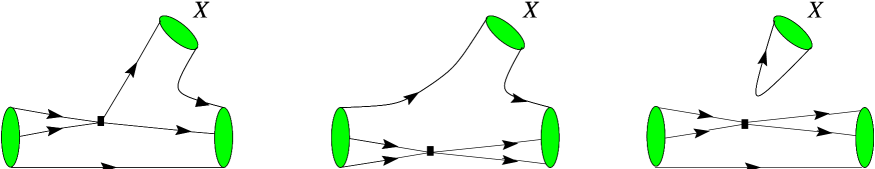
Figure 3: The different topologies for pseudo-annihilation contributions to $b$ baryon decays.

5 Escaping suppression by factorization breaking

The idea of this paper is to study the size and pattern of corrections to factorization in an environment where they are not “hidden” behind a larger factorizing piece. Without giving an exhaustive discussion of nonfactorizing contributions, we now consider two of them and see why the various suppression mechanisms discussed in Sect. 3.1 do not apply.

5.1 Nonfactorizing gluon exchange

Naive factorization is broken by strong interactions of the quarks originating from the $b$ decay. In the language of quarks and gluons they correspond to diagrams like the ones in Fig. 4. What is important in our context is that such contributions no longer involve the matrix elements of the meson $X$ with the local currents $V$, $A$, $S$, $P$. As a consequence the suppression mechanisms based on the smallness of the decay constant $f_{X}$ are not effective. Also, one or several gluons absorbed by the quark-antiquark pair that will form $X$ can transfer both helicity and orbital angular momentum, so that the spin of $X$ is no longer restricted to be 0 or 1.

Note that these arguments are independent on whether the internal lines in the diagrams of Fig. 4 have large virtualities or not. In the first case the corresponding contributions can be calculated in perturbation theory. In Sect. 6 we will analyze them in the QCD factorization approach and explicitly see that our suppression mechanisms are no longer operative.

If the internal lines in these diagrams are not hard, perturbation theory is not reliable, and other descriptions of the corresponding reactions might be more adequate. If one treats them for instance as hadronic rescattering, there is again no reason why final state mesons $X$ with small decay constants or higher spin should be suppressed.

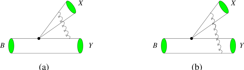
Figure 4: Examples of diagrams with gluon exchange breaking naive factorization: (a) vertex correction, (b) spectator interaction.

5.2 Annihilation contributions

Annihilation diagrams are another important contribution violating naive factorization. In Tables 2 and 3 we have indicated the channels where they can occur, either from tree level $W$ exchange or from penguin operators. An indication of the importance of annihilation could be obtained from data by comparing decays with and without such contributions that are otherwise similar, for instance $\bar{B}^{0}\to D^{+}a_{0}^{-}$ and $\bar{B}_{s}\to D_{s}^{+}a_{0}^{-}$, or $B^{-}\to\pi^{0}D_{sJ}^{-}$ and $B^{-}\to\eta D_{sJ}^{-}$.

Depending on the flavor structure of the decay there are three annihilation topologies. The one shown in Fig. 5a is for example relevant for $\bar{B}^{0}\to D^{+}a_{0}^{-}$ and for $B^{-}\to\pi^{-}\bar{K}_{2}^{*0}$. In this case only one of the quarks forming our candidate meson $X$ originates from the effective weak vertex, so that our suppression mechanisms are not relevant. Notice that this holds true irrespective of whether the interactions between the $q\bar{q}$-pair and the quarks attached to the decay vertex are under perturbative control or not, a point that is controversial in the literature [8, 9].

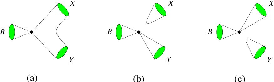
Figure 5: The different topologies for annihilation contributions to decays $B\to YX$, where $X$ is one of our candidate mesons given in Table 1.

The two remaining topologies correspond to Zweig forbidden contributions. Neglecting electromagnetic interactions, they require that the meson formed from the $q\bar{q}$-pair has isospin $I=0$. In Fig. 5b, relevant for our decays into charmonium, neither of the quarks from the annihilation vertex enters in $X$, so that our suppression mechanisms again do not apply. Finally, there is the case of Fig. 5c, where $X$ is formed from the quarks of the decay vertex. Our suppression mechanisms only apply here if the $\bar{q}q$-pair interacts solely with the quarks in the $B$ meson, but not with the ones forming the meson $X$.

The topologies for pseudo-annihilation contributions in $b$ baryon decays have already been shown in Fig. 3. All of them circumvent suppression.

6 The case of QCD factorization

In the QCD factorization approach developed by Beneke et al. [6, 7, 8], those corrections to naive factorization that are dominated by hard gluon exchange are calculated in perturbation theory, all other contributions are found to be power suppressed in $1/m_{b}$. The physical mechanism underlying these results is color transparency of the meson ejected by the effective weak current. QCD factorization can therefore not be applied to decays where a $D$ meson with its highly asymmetric quark-antiquark configurations is emitted from the current, and we will thus not consider the corresponding channels in this section.

As QCD factorization relies on color transparency, it also requires the emitted meson to be fast in the $B$ rest frame. Certain types of power corrections will therefore increase with the mass $m_{X}$ of the emitted meson. One can reduce the bias due to such effects by comparing our suppressed decays with unsuppressed channels involving mesons of similar mass. Examples are the $\rho(770)$, $a_{1}(1260)$, or $\rho(1450)$ for isospin-one mesons, and the $K^{*}$ and $K_{1}$ resonances for the strange sector.

6.1 Distribution amplitudes

The most important effect of radiative corrections in our context is that the currents like $\langle{X}|\,{\bar{d}(0)\gamma^{\mu}(1-\gamma_{5})u(0)}\,|0\rangle$ occurring in naive factorization become nonlocal. The leading configurations in $1/m_{b}$ involve light-like separations $z$ and are parameterized by meson distribution amplitudes. In light-cone gauge, they read for a $d\bar{u}$ meson

$$\langle{X(q,J_{3}=0)}|\,{\bar{d}(z)\,\gamma^{\mu}(\gamma_{5})u(-z)}\,|0\rangle\Big{|}_{z^{2}=0}=-iq^{\mu}\int_{0}^{1}du\,e^{i(2u-1)\,q\cdot z}\,\varphi(u)+\ldots$$ (25)

to twist-two accuracy, where the $\ldots$ stand for terms of twist three and higher, which contribute to hard processes only at the power correction level. The Dirac matrices $\gamma^{\mu}$ and $\gamma^{\mu}\gamma_{5}$ are to be taken for mesons with natural and unnatural parity, $P=(-1)^{J}$ and $P=(-1)^{J+1}$, respectively. The variable $u$ gives the momentum fraction carried by the quark in the meson $X$, a natural frame of reference in our case being the $B$ rest frame. Notice that the twist-two distribution amplitudes involving the vector and axial currents select the polarization state with zero angular momentum $J_{3}$ along $\vec{q}$ in that frame. We remark that our subsequent discussion remains valid if instead of a meson $X$ one considers a continuum final state with appropriate quantum numbers as discussed in Sect. 3.4. In this case $\varphi$ is to be replaced with a generalized distribution amplitude [22], defined as in Eq. (25) with the appropriate replacement of state vectors $|X\rangle$.

One easily sees that the lowest moment of $\varphi$ in $u$ gives back the local currents, so that for mesons with spin 0 or 1 one recovers the decay constant,

$$\int_{0}^{1}du\,\varphi(u)=f_{X}.$$ (26)

The nonlocal currents in Eq. (25) have however matrix elements for mesons of any spin $J$. Taylor expanding the bilocal operators around $z=0$ gives in fact operators with arbitrarily high numbers of partial derivatives between $\bar{d}(0)$ and $u(0)$, and thus with arbitrarily high spin. In other words the lowest moment $\int du\,\varphi(u)$ of the distribution amplitude, projecting out the local $V$ or $A$ current, vanishes for mesons with $J\geq 2$, but not the function $\varphi(u)$ itself. Hence the production of mesons with spin 2 and higher is no longer forbidden at the level of $\alpha_{s}$ corrections to naive factorization. We thus find an explicit realization of our arguments in Sect. 5.1: gluon exchange such as in Fig. 4 indeed makes the production of higher-spin mesons possible.

Let us now see what becomes of the other suppression mechanisms we discussed in Sect. 3.1. Charge conjugation invariance implies that the distribution amplitudes $\varphi_{X_{0}}$ for the neutral $a_{0}$ and $b_{1}$ mesons are odd under the exchange of quark and antiquark momenta, $\varphi_{X^{0}}(u)=-\varphi_{X^{0}}(1-u)$, so that their first moment  (26) is zero. In the exact isospin limit, the distribution amplitudes for the charged and neutral mesons in an isotriplet are the same, so that with Eq. (26) the decay constants of the charged $a_{0}$ and $b_{1}$ have to vanish, as already seen in Sect. 3.1. In the real world, the part of the distribution amplitude that is even under $u\to 1-u$ is therefore small for the charged $a_{0}$ and $b_{1}$, i.e., $\varphi_{X^{-}}(u)+\varphi_{X^{-}}(1-u)\sim m_{d}-m_{u}$. This does however not restrict the odd part of $\varphi_{X^{-}}(u)$, which can be comparable in size to the distribution amplitudes of, say, the $\pi$ or the $\rho$. Considering the distribution amplitude of the $K_{0}^{*}$ and using SU(3) symmetry we see that its even part is suppressed by $m_{s}-m_{u}$, but not its odd part.

Along the same lines of reasoning, we find that up to isospin breaking effects the distribution amplitudes for the charged heavy pions are even under $u\to 1-u$. The lowest moment $\int du\,\varphi_{\pi(1300)}(u)$ is small of order $m_{u}+m_{d}$ according to Eqs. (12) and (26), but there is no such restriction on higher even moments such as $\int du\,(2u-1)^{2}\,\varphi_{\pi(1300)}(u)$. We thus see that neither spin nor any of our other suppression mechanisms applies at the level of $\alpha_{s}$ corrections.

It is useful to expand the distribution amplitude in Gegenbauer polynomials $C_{n}^{3/2}$, which are the eigenfunctions of the leading-order evolution equation [23] for quark distribution amplitudes. In order to achieve a uniform notation for mesons with different spins we write

$$\varphi(u;\mu)=f^{\varphi}\,6u(1-u)\Big{[}B_{0}+\sum_{n=1}^{\infty}B_{n}(\mu)\,C_{n}^{3/2}(2u-1)\Big{]},$$ (27)

where we have explicitly displayed the dependence on the factorization scale $\mu$. For mesons $X$ with spin 0 or 1, we have $B_{0}=1$ and $f^{\varphi}$ is just the decay constant $f_{X}$, whereas for mesons with $J\geq 2$ we have $B_{0}=0$. We will in the following only use products $f^{\varphi}B_{n}$ so that we need not specify the separate normalizations of $f^{\varphi}$ and $B_{n}$ in that case. From our above discussion it follows that for our candidate mesons one or more of the lowest coefficients in the expansion (27) are either zero or small of order $m_{d}-m_{u}$, $m_{d}+m_{u}$, or $m_{s}-m_{u}$. In the Appendix we will estimate the orders of magnitude of the leading coefficients to be

$$|f^{\varphi}B_{1}|_{a_{0},b_{1},a_{2},K_{0}^{*},K_{2}^{*}} \approx 75~{}\mbox{MeV},$$

$$|f^{\varphi}B_{2}|_{\pi(1300),\pi_{2},\rho_{3}} \approx 50~{}\mbox{MeV},$$ (28)

evaluated at the renormalization scale $\mu=m_{b}=4.4$ GeV.

6.2 Decays into a $D$ and a light meson $X$

For these channels the only diagrams one needs to consider at leading order in $1/m_{b}$ are vertex corrections such as in Fig. 4a. The result of the $O(\alpha_{s})$ calculation for the matrix element of the effective weak Hamiltonian can be written as the sum of

$$\langle D^{+}X^{-}|{\cal H}_{\mathrm{eff}}|\bar{B}^{0}\rangle^{\mathrm{corr}} = -i\,\frac{G_{F}}{\sqrt{2}}V_{cb}^{\phantom{*}}V_{ud}^{*}\;a_{1}^{\mathrm{corr}}f^{\varphi}\,q_{\mu}\langle D^{+}|\bar{c}\gamma^{\mu}b|\bar{B}^{0}\rangle,$$

$$\langle D^{*+}X^{-}|{\cal H}_{\mathrm{eff}}|\bar{B}^{0}\rangle^{\mathrm{corr}} = i\,\frac{G_{F}}{\sqrt{2}}V_{cb}^{\phantom{*}}V_{ud}^{*}\;a_{1}^{\mathrm{corr}}f^{\varphi}\,q_{\mu}\langle D^{*+}|\bar{c}\gamma^{\mu}\gamma_{5}b|\bar{B}^{0}\rangle,$$ (29)

and the contribution of naive factorization, taken with a coefficient $a_{1}^{\mathrm{fact}}$ which equals the coefficient $a_{1}$ of Sect. 2 evaluated at next-to leading order, up to a small term removing the renormalization scheme dependence. For details we refer to Eqs. (95) and (96) of [7]. The coefficients $a_{1}^{\mathrm{corr}}$ are given by

$$f^{\varphi}a_{1}^{\mathrm{corr}}=\frac{\alpha_{s}(\mu)}{4\pi}\,C_{2}(\mu)\,\frac{C_{F}}{N_{c}}\,\int_{0}^{1}du\,F(u,\pm z)\,\varphi(u;\mu),$$ (30)

where the function $F(u,z)$ with $z=m_{c}/m_{b}$ can be found in [7]. Its second argument is $+z$ for decays into $D$ and $-z$ for decays into $D^{*}$, with $z=m_{c}/m_{b}$, so that $a_{1}^{\mathrm{corr}}$ depends on both mesons in the final state. Its dependence on the distribution amplitude of $X$ can be expressed as

$$a_{1}^{\mathrm{corr}}(\mu)=a_{1}^{(0)}(\mu)\,B_{0}+\sum_{n=1}^{\infty}a_{1}^{(n)}(\mu)\,B_{n}(\mu).$$ (31)

The first few coefficients $a_{1}^{(n)}$ are listed in Table 5. We see that they are small compared with 1, and that they tend to decrease with $n$. They depend substantially on the renormalization scale $\mu$. One finds

$$\frac{a_{1}^{(n)}(m_{b}/2)}{a_{1}^{(n)}(m_{b})}\approx\frac{a_{1}^{(n)}(m_{b})}{a_{1}^{(n)}(2m_{b})}\approx 2,$$ (32)

a falloff mostly due to the Wilson coefficient $C_{2}$. The Gegenbauer coefficients $B_{n}$ also decrease with the factorization scale, although by less than a factor 1.2 for $B_{1}$ and $B_{2}$ when $\mu$ is varied between $m_{b}/2$ and $m_{b}$ or between $m_{b}$ and $2m_{b}$. The effects of this dependence on $\mu$ are quite mild for decays where most of the result is due to the Born level term $f^{\varphi}a_{1}^{\mathrm{fact}}$, but not for our decays where this contribution is absent or suppressed by a small value of $f^{\varphi}$. A more stable prediction would require the inclusion of $O(\alpha_{s}^{2})$ corrections. Since they involve again the color allowed Wilson coefficient $C_{1}$ they may actually not be small compared with the $O(\alpha_{s})$ terms.

	$a_{1}^{(0)}$	$a_{1}^{(1)}$	$a_{1}^{(2)}$	$a_{1}^{(3)}$	$a_{1}^{(4)}$
$\bar{B}^{0}\to D^{+}X^{-}$	$12.3+12.7i$	$-8.1+17.8i$	$1.7-0.8i$	$-2.3+4.9i$	$\hfill 0.3-0.5i$
$\bar{B}^{0}\to D^{*+}X^{-}$	$11.7+8.4i\hfill$	$-9.5+16.0i$	$0.3-1.2i$	$-3.2+5.0i$	$-0.2-0.2i$

Table 5: The first few coefficients $a_{1}^{(n)}$ of the expansion (31) in units of $10^{-3}$. They are evaluated at renormalization scale $\mu=m_{b}=4.4$ GeV with input parameters $\Lambda^{(5)}_{\overline{\mathrm{MS}}}=220$ MeV and $m_{c}/m_{b}=0.3$. With the same parameters one has $a_{1}^{\mathrm{fact}}=1.039$.

Whereas $a_{1}^{\mathrm{fact}}$ is real valued, we observe from Eq. (31) and Table 5 that $a_{1}^{\mathrm{corr}}$ is complex. The strong phases of unsuppressed channels like $\bar{B}^{0}\to D^{+}\pi^{-}$ are thus small in QCD factorization. On the contrary, they can be sizeable in our suppressed decays, where $\alpha_{s}$ contributions are essential.

6.3 Decays into charmonium

The radiative corrections to factorization for decays into charmonium states have not been calculated yet. The following observation [7] is however relevant in our context. The naive factorization formula for these decays involves the color suppressed coefficient $a_{2}$ and color suppressed penguins, but at the level of loop corrections the color allowed coefficient $C_{1}$ will come in. Hence the $O(\alpha_{s})$ terms will probably be sizeable compared with the naive factorization result. This expectation is supported by an analysis of inclusive $B$ decays into charmonium [24]. Whereas naive factorization forbids the decays of Table 3 into a $\chi_{c0}$ or a $\chi_{c2}$ instead, one may then expect that within QCD factorization their branching ratios are not much smaller or even of similar size than for the corresponding decays into $J/\Psi$ or $\chi_{c1}$.

6.4 Decays into two light mesons

For these channels, not only vertex corrections need to be considered, but also so-called penguin contractions (cf. Fig. 7 of [7]) and hard interactions with the spectator quark from the $B$ as shown in Fig. 4b. The latter involve the twist-two distribution amplitudes $\varphi_{Y}$ and $\varphi_{X}$ of both final state mesons. Mesons with $J\geq 1$ have a second twist-two distribution amplitude [25] involving the nonlocal tensor current $\bar{d}(z)\,\sigma^{\mu\nu}u(-z)$, which describes states with helicity $J_{3}=\pm 1$ and can also contribute now.

Beyond the level of leading twist contributions, several power corrections have been considered in the literature [8, 26]. A particular type of correction that is numerically not suppressed occurs for final-state mesons with spin $J=0$ and involves their twist-three distribution amplitudes defined from the nonlocal (pseudo)scalar and tensor currents [27]. Their contribution to the amplitude relative to the twist-two radiative corrections is controlled by the ratio $r$ defined as in (22), which is formally of order $1/m_{b}$ but numerically not small. With the quark mass values we use, one has $r_{\pi}=r_{K}=1$, and the corresponding twist-three radiative corrections have size similar to the leading-twist ones. This is also the case for the $a_{0}$, $\pi(1300)$, and $K_{0}^{*}$ mesons we are considering here. Indeed, the twist-two distribution amplitudes are comparable in size for $a_{0}$, $\pi(1300)$, $K_{0}^{*}$, and $\pi$, $K$, as follows from comparing our estimates (28) with $f_{\pi}$ or $f_{K}$. The same holds for the respective twist-three distribution amplitudes, which are controlled by the local (pseudo)scalar matrix elements in Eqs. (19) and (20). We recall that the twist-three pieces just discussed can only be estimated in QCD factorization because they lead to logarithmic divergences at the endpoints of the distribution amplitudes.

Logarithmic endpoint divergences also appear in annihilation contributions, which in the power counting scheme of QCD factorization are again $1/m_{b}$ corrections, even for those terms involving only twist-two distribution amplitudes. In a recent study of decays $B\to\pi\pi$ and $B\to\pi K$ Beneke et al. [8] estimated annihilation contributions to be moderate corrections to the leading terms computed in the QCD factorization framework, giving a benchmark number of 25% in the branching ratio, although with large uncertainties. Notice that the small parameter controlling the relative weight of annihilation and leading contributions in their calculation is

$$\frac{f_{B}f_{Y}}{(m_{B}^{2}-m_{Y}^{2})F_{0}^{B\to Y}(m_{X}^{2})},$$ (33)

which depends only mildly on the mass of the emitted meson through the $B\to Y$ transition form factor. We take this as an indication that the importance of annihilation contributions is not primarily driven by the size of $m_{X}$.

We expect then that in decays such as $\bar{B}^{0}\to a_{0}^{+}a_{0}^{-}$ the hard nonfactorizable terms calculable in QCD factorization, and possibly also the power corrections estimated there should be small compared to the amplitude for $\bar{B}^{0}\to\pi^{+}\pi^{-}$, which is dominated by the contribution of the large coefficient $a_{1}$.

For penguin dominated decays like $B\to\pi K$, the overall size of corrections found in Ref. [8] is not so small compared with the result of the naive factorization formula. With the “designer” modes $\bar{B}^{0}\to\pi^{+}K_{2}^{*-}$ and $B^{-}\to\pi^{-}\bar{K}_{2}^{*0}$ we can isolate such nonfactorizable terms. Among these, annihilation contributions from scalar penguin operators are of special interest. In QCD factorization they are a power correction, but not in the PQCD approach, where Keum et al. [9] found that they contribute at order one and with a large phase to the $B\to\pi K$ decay amplitudes. Comparing the branching ratios of the above decays into $K_{2}^{*}$ with those into a $K$ or $K^{*}$ can show whether scalar penguin annihilation contributions are indeed large.

7 Branching ratio estimates for decays $B\to DX$

We present now our numerical estimates of the branching ratios for decays $\bar{B}^{0}\to D^{+}X^{-}$, where $X$ is one of $a_{0}$, $a_{2}$, $b_{1}$, $\pi(1300)$, $\pi_{2}$, $\rho_{3}$, or $K_{0}^{*}(1430)$, $K_{2}^{*}$. As discussed in Sect. 6.2, these channels receive hard gluon corrections to naive factorization, which can be calculated in the QCD factorization approach.

We recall that for the $a_{2}$, $\pi_{2}$, $\rho_{3}$, and $K_{2}^{*}$, the tree term proportional to $a_{1}^{\mathrm{fact}}$ is absent. The contribution from the $\alpha_{s}$ correction $a_{1}^{\mathrm{corr}}$ given in (29) involves a contraction of $q_{\mu}$ with the matrix element parameterized as

$$\langle D(p^{\prime})|\bar{c}\gamma^{\mu}b|\bar{B}(p)\rangle = F_{1}(q^{2})\left\{(p+p^{\prime})^{\mu}-\frac{m_{B}^{2}-m_{D}^{2}}{q^{2}}\,q^{\mu}\right\}+F_{0}(q^{2})\,\frac{m_{B}^{2}-m_{D}^{2}}{q^{2}}\,q^{\mu},$$ (34)

where $q=p-p^{\prime}$. One easily sees that the $\alpha_{s}$ contributions always pick up the form factor $F_{0}$, independent of the spin of $X$. Thus, the decay rate for our candidates $X$, as well as for any other spin zero meson like the $\pi$, can be written as

$$\Gamma(\bar{B}^{0}\to D^{+}X^{-}) = \frac{G_{F}^{2}}{16\pi}\,\frac{(m_{B}^{2}-m_{D}^{2})^{2}}{m_{B}^{2}}\,p_{X}\,\Big{|}V^{\phantom{*}}_{cb}V_{ud}^{*}\Big{|}^{2}\;\Big{|}\,f^{\varphi}(a_{1}^{\mathrm{fact}}+a_{1}^{\mathrm{corr}})\,F_{0}(m_{X}^{2})\,\Big{|}^{2},$$ (35)

where $p_{X}$ denotes the magnitude of the three-momentum of $X$ in the $B$ rest frame.

We normalize the rate of the decays into $X$ to the unsuppressed one into a light pion. This has the advantage that the CKM factors cancel (except for the strange mesons) and that we can use the measured branching ratio for $\bar{B}^{0}\to D^{+}\pi^{-}$ decays, where naive factorization works well [2, 7]. For the ratio of decay rates we have the simple expression

$$\frac{\Gamma(\bar{B}^{0}\to D^{+}X^{-})}{\Gamma(\bar{B}^{0}\to D^{+}\pi^{-})}\approx\left|\,\frac{f^{\varphi}(a_{1}^{\mathrm{fact}}+a_{1}^{\mathrm{corr}})}{f_{\pi}a_{1}^{\mathrm{fact}}}\,\right|^{2},$$ (36)

where for simplicity we have neglected the term $a_{1}^{\mathrm{corr}}$ for the $\pi^{-}$, where its effect is of order 1% to 2%. Eq. (36) has corrections due to phase space and the evaluation of the form factor $F_{0}$ at different momentum transfer $q^{2}$, which go in opposite directions. The relevant $q^{2}$ ranges from roughly 1 GeV² for the $a_{0}(980)$ to 3 GeV² for the $\pi_{2}$ and $\rho_{3}$, to be compared with $q^{2}\approx 0$ for the $\pi$. We have checked that the relation (36) is affected by these mass effects by not more than 10% to 15%. This is sufficient in our context, given the dominant theoretical uncertainty of our calculation hidden in the decay constants and distribution amplitudes. For $X=K_{0}^{*}(1430)$, $K_{2}^{*}$ we have to include a CKM factor $|V_{us}/V_{ud}|^{2}$, which is known to a good precision. In our numerical analysis we take $|V_{us}/V_{ud}|=0.23$ from [11].

We evaluate (36) using the expansion (31) with the coefficients $a_{1}^{(n)}$ of Gegenbauer moments in Table 5, the estimates (28) for the Gegenbauer moments $B_{n}$, and the maximal values of the decay constants in (14) to (17). The $b_{1}$ can have a small decay constant, for which we are not aware of any information in the literature, and in our calculation we set it to zero. Before presenting the branching ratios let us study the magnitude of the individual terms entering in (36). We have $f_{\pi}a_{1}^{\mathrm{fact}}=136$ MeV for the pion, and for the mesons with leading Gegenbauer moments $f^{\varphi}B_{1}$ and $f^{\varphi}B_{2}$, we respectively obtain

$$|f^{\varphi}a_{1}^{\mathrm{corr}}\,|_{a_{0},b_{1},a_{2},K_{0}^{*},K_{2}^{*}} = 1.5~{}\mbox{MeV},$$

$$|f^{\varphi}a_{1}^{\mathrm{corr}}\,|_{\pi(1300),\pi_{2},\rho_{3}} = 0.1~{}\mbox{MeV},$$ (37)

at renormalization scale $\mu=m_{b}$. The second term is tiny mainly because of the small coefficient $a_{1}^{(2)}$ from the one-loop calculation. Since our estimate in the Appendix does not yield the sign of $f^{\varphi}B_{n}$, we have a twofold ambiguity when adding $f^{\varphi}a_{1}^{\mathrm{corr}}$ to $f^{\varphi}a_{1}^{\mathrm{fact}}$, and find

$$f_{a0(980)}\,a_{1}^{\mathrm{fact}} = 2.6\mbox{~{}MeV},\hskip 30.00005pt|f^{\varphi}(a_{1}^{\mathrm{fact}}+a_{1}^{\mathrm{corr}})\,|_{a0(980)}\hskip 5.50003pt\,=\;2.4\mbox{~{}or~{}}3.5\mbox{~{}MeV},$$

$$f_{a0(1450)}\,a_{1}^{\mathrm{fact}} = 0.7\mbox{~{}MeV},\hskip 30.00005pt|f^{\varphi}(a_{1}^{\mathrm{fact}}+a_{1}^{\mathrm{corr}})\,|_{a0(1450)}\hskip 2.5pt\,=\;1.3\mbox{~{}or~{}}1.9\mbox{~{}MeV},$$

$$f_{\pi(1300)}\,a_{1}^{\mathrm{fact}} = 7.5\mbox{~{}MeV},\hskip 30.00005pt|f^{\varphi}(a_{1}^{\mathrm{fact}}+a_{1}^{\mathrm{corr}})\,|_{\pi(1300)}\hskip 5.50003pt\,=\;7.4\mbox{~{}or~{}}7.6\mbox{~{}MeV},$$

$$f_{K_{0}^{*}(1430)}\,a_{1}^{\mathrm{fact}} = \;48\mbox{~{}MeV},\hskip 30.00005pt|f^{\varphi}(a_{1}^{\mathrm{fact}}+a_{1}^{\mathrm{corr}})\,|_{K_{0}^{*}(1430)}\,=\;\;47\mbox{~{}or~{}}\,48\mbox{~{}MeV}.$$ (38)

Notice the enormous correction to the naive factorization result for the $a_{0}(1450)$. The impact of nonfactorizing corrections is similarly strong for the $a_{0}(980)$ if we take the minimum value $f_{a_{0}(980)}=0.7$ MeV from Eq. (15). For the $\pi(1300)$, nonfactorizing terms remain always moderate since $|f^{\varphi}a_{1}^{\mathrm{corr}}|_{\pi(1300)}$ is small even compared with the lowest estimate of $f_{\pi(1300)}$ in Eq. (16). The $K_{0}^{*}$ has a decay constant much larger than $|f^{\varphi}a_{1}^{\mathrm{corr}}|_{K_{0}^{*}}$ and is the only case where the corrections hardly matter.

Using ${\cal{B}}(B^{0}\to D^{-}\pi^{+})=(3.0\pm 0.4)\cdot 10^{-3}$ from [11] and the maximal values in (38), we obtain the branching ratios in Table 6. To show their dependence on the choice of renormalization scale, we give them for $\mu=m_{b}$ and $\mu=m_{b}/2$. We take the latter as an indication of how large the branching ratios can be in QCD factorization, although they are not upper bounds in a rigorous sense. We also show the corresponding results from naive factorization, where for consistency of comparison we have again neglected the corrections discussed below Eq. (36). Here the scale dependence is minute, less than 2 percent, and the values in Table 6 are those for $\mu=m_{b}$.

decay mode	naive factorization	QCD factorization
		$\mu=m_{b}$	$\mu=m_{b}/2$
$\bar{B}^{0}\to D^{+}a_{0}(980)$	$1.1\cdot 10^{-6}$	$2.0\cdot 10^{-6}$	$4.0\cdot 10^{-6}$
$\bar{B}^{0}\to D^{+}a_{0}(1450)$	$8.6\cdot 10^{-8}$	$5.8\cdot 10^{-7}$	$2.1\cdot 10^{-6}$
$\bar{B}^{0}\to D^{+}b_{1},\,D^{+}a_{2}$	0	$3.5\cdot 10^{-7}$	$1.7\cdot 10^{-6}$
$\bar{B}^{0}\to D^{+}\pi(1300)$	$9.1\cdot 10^{-6}$	$9.3\cdot 10^{-6}$	$9.6\cdot 10^{-6}$
$\bar{B}^{0}\to D^{+}\pi_{2},\,D^{+}\rho_{3}$	0	$1.4\cdot 10^{-9}$	$8.1\cdot 10^{-9}$
$\bar{B}^{0}\to D^{+}K^{*}_{0}(1430)$	$2.0\cdot 10^{-5}$	$2.0\cdot 10^{-5}$	$2.1\cdot 10^{-5}$
$\bar{B}^{0}\to D^{+}K^{*}_{2}$	0	$1.9\cdot 10^{-8}$	$9.2\cdot 10^{-8}$
$\bar{B}^{0}\to D^{*+}a_{0}(980)$	$1.0\cdot 10^{-6}$	$1.8\cdot 10^{-6}$	$3.7\cdot 10^{-6}$
$\bar{B}^{0}\to D^{*+}a_{0}(1450)$	$7.9\cdot 10^{-8}$	$5.2\cdot 10^{-7}$	$1.9\cdot 10^{-6}$
$\bar{B}^{0}\to D^{*+}b_{1},\,D^{*+}a_{2}$	0	$2.9\cdot 10^{-7}$	$1.5\cdot 10^{-6}$
$\bar{B}^{0}\to D^{*+}\pi(1300)$	$8.3\cdot 10^{-6}$	$8.4\cdot 10^{-6}$	$8.4\cdot 10^{-6}$
$\bar{B}^{0}\to D^{*+}\pi_{2},\,D^{*+}\rho_{3}$	0	$5.7\cdot 10^{-10}$	$3.2\cdot 10^{-9}$
$\bar{B}^{0}\to D^{*+}K^{*}_{0}(1430)$	$1.8\cdot 10^{-5}$	$1.9\cdot 10^{-5}$	$1.9\cdot 10^{-5}$
$\bar{B}^{0}\to D^{*+}K^{*}_{2}$	0	$1.5\cdot 10^{-8}$	$7.7\cdot 10^{-8}$

Table 6: Branching ratios for various decay modes obtained in QCD factorization for two choices of the renormalization scale $\mu$. For comparison we also give the branching ratios in the naive factorization approach. We recall that we have set $f_{b_{1}}=0$ for lack of better knowledge.

We proceed to decays into a vector meson, $\bar{B}^{0}\to D^{*+}X^{-}$. The contraction of $q_{\mu}$ with the matrix element $\langle D^{*}|\bar{c}\gamma^{\mu}\gamma_{5}b|\bar{B}\rangle$ depends again only on a single form factor, commonly referred to as $A_{0}$ and defined e.g. in [3]. The decay rate is then given by

$$\Gamma(\bar{B}^{0}\to D^{*+}X^{-}) = \frac{G_{F}^{2}}{4\pi}\,p_{X}^{3}\,|V^{\phantom{*}}_{cb}V_{ud}^{*}|^{2}\,\Big{|}f^{\varphi}(a_{1}^{\mathrm{fact}}+a_{1}^{\mathrm{corr}})\,A_{0}(m_{X}^{2})\,\Big{|}^{2}.$$ (39)

As mentioned in Sect. 6.2, the coefficients $a_{1}^{\mathrm{corr}}$ for decays into $D^{*}$ are different from those into $D$, and we now have

$$|f^{\varphi}(a_{1}^{\mathrm{fact}}+a_{1}^{\mathrm{corr}})\,|_{a0(980)} = 2.2\mbox{~{}or~{}}3.5\mbox{~{}MeV},$$

$$|f^{\varphi}(a_{1}^{\mathrm{fact}}+a_{1}^{\mathrm{corr}})\,|_{a0(1450)} = 1.2\mbox{~{}or~{}}1.9\mbox{~{}MeV},$$

$$|f^{\varphi}(a_{1}^{\mathrm{fact}}+a_{1}^{\mathrm{corr}})\,|_{\pi(1300)} = 7.5\mbox{~{}MeV},$$

$$|f^{\varphi}(a_{1}^{\mathrm{fact}}+a_{1}^{\mathrm{corr}})\,|_{K_{0}^{*}(1430)} = 47\mbox{~{}or~{}}49\mbox{~{}MeV}$$ (40)

at $\mu=m_{b}$. The analogous expression for the ratio (36) of decay rates still holds, although with different mass corrections. We estimate them to be not much larger than for the $D$ and neglect them as before. Normalizing to ${\cal{B}}(B^{0}\to D^{*-}\pi^{+})=(2.76\pm 0.21)\cdot 10^{-3}$ from [11] we obtain the branching ratios in Table 6, which are somewhat smaller than the corresponding ones for decays into the $D$. With the exception of decays into $K^{*}_{2},\pi_{2}$, or $\rho_{3}$, all estimated branching ratios are larger than $10^{-7}$ and within experimental reach at the $B$-factories. We expect similar branching ratios for $B_{s}$ decays into $D_{s}^{(*)}$ and the same candidate mesons $X$, up to SU(3) breaking effects.

To facilitate comparison of the branching ratios of Table 6 into $K_{0}^{*}$ and $K_{2}^{*}$ with those into a $K$, we estimate the latter as

$${\cal{B}}(\bar{B}^{0}\to D^{+}K^{-}) \simeq \frac{f^{2}_{K}}{f_{\pi}^{2}}\left|\frac{V_{us}}{V_{ud}}\right|^{2}{\cal{B}}(\bar{B}^{0}\to D^{+}\pi^{-})=(2.4\pm 0.3)\cdot 10^{-4}\,,$$

$${\cal{B}}(\bar{B}^{0}\to D^{*+}K^{-}) \simeq \frac{f^{2}_{K}}{f_{\pi}^{2}}\left|\frac{V_{us}}{V_{ud}}\right|^{2}{\cal{B}}(\bar{B}^{0}\to D^{*+}\pi^{-})=(2.2\pm 0.2)\cdot 10^{-4}\,,$$ (41)

which is in good agreement with data on the ratios ${\cal{B}}(\bar{B}^{0}\to D^{+}K^{-})/{\cal{B}}(\bar{B}^{0}\to D^{+}\pi^{-})=0.079\pm 0.011$ and ${\cal{B}}(\bar{B}^{0}\to D^{*+}K^{-})/{\cal{B}}(\bar{B}^{0}\to D^{*+}\pi^{-})=0.074\pm 0.016$ reported in [28].

A considerable source of uncertainty in our decay rate estimates are the unknown meson decay constants and distribution amplitudes. Let us illustrate this for the channel $\bar{B}^{0}\to D^{+}a_{0}(980)$. With the minimal value of $f_{a_{0}(980)}$ in Eq. (14) we obtain $|f^{\varphi}(a_{1}^{\mathrm{tree}}+a_{1}^{\mathrm{corr}})|_{a0(980)}=\mbox{1.3 or 1.9~{}MeV}$ at $\mu=m_{b}$. The larger of the two possibilities corresponds to a branching ratio ${\cal{B}}(\bar{B}^{0}\to D^{+}a_{0}(980))=5.8\cdot 10^{-7}$, about three times smaller than the corresponding one in Table 6.

We have already seen the sensitivity of our results on the choice of renormalization scale. This uncertainty is largest for the branching ratios which are zero in naive factorization, with a variation by a factor of 5 to 6 between $\mu=m_{b}$ and $\mu=m_{b}/2$. How important it is for the other channels depends on the actual size of the decay constants and distribution amplitudes. We also remark that the reliability of the QCD factorization approach for our “light” mesons with masses in the range from 1 to 1.7 GeV might be questionable, at least unless finite-mass corrections can be taken into account.

Most important, however, is that the hard nonfactorizing contributions are small on the scale of the amplitudes for unsuppressed decays. With all uncertainties discussed above we find that $f^{\varphi}a_{1}^{\mathrm{corr}}$ is at most a few MeV, i.e., less than 5% of $f_{\pi}a_{1}^{\mathrm{fact}}$. One may well expect that soft corrections (or annihilation graphs when they can occur) are bigger than the hard ones. For all our meson candidates except the $K_{0}^{*}$ they would then lead to considerably larger branching ratios than we have estimated.

The decays into $K_{0}^{*}$ are different in this context. Here the perturbative corrections to the prediction of naive factorization are quite small and their uncertainties less relevant, and further soft corrections might or might not overshadow the factorizing piece. Once the decay constant of the $K_{0}^{*}$ is known experimentally, one should of course refine our estimates by taking into account the phase space and form factor corrections in (36).

7.1 Background from $B^{0}$ decay

We see in Fig. 2 that the same final state of our signal mode $\bar{B}^{0}\to D^{+}X^{-}$ just discussed can be produced in the decay of the $C\!P$ conjugated parent meson, $B^{0}\to D^{+}X^{-}$. As mentioned in Sect. 4, this background is CKM suppressed with respect to the signal. On the other hand, the signal mode is punished by a small decay constant, whereas the background goes with $f_{D}\sim 200$ MeV. One expects the background-to-signal ratio to be large, since at the amplitude level $\lambda^{2}f_{D}/f_{X}\sim{\cal{O}}(1)$. We recall that no such background exists in decays into a strange final state, $\bar{B}^{0}\to D^{+}X_{s}^{-}$ or $\bar{B}_{s}\to D_{s}^{+}X^{-}$.

The background to $\bar{B}^{0}\to D^{+}X^{-}$ can of course be removed by flavor tagging. Experimental discrimination between $B$ and $\bar{B}$ is however challenging in decays with branching ratios of less than $10^{-5}$, and it is worthwhile to see how far one can go without a flavor tag. Let us therefore investigate in more detail the branching ratios of the background decays for the case of the $a_{0}$. We parameterize the matrix element for the $B\to a_{0}$ transition in terms of form factors $F_{0}^{a}$ and $F_{1}^{a}$ as

$$\langle a_{0}(p^{\prime})|\bar{u}\gamma^{\mu}\gamma_{5}b|\bar{B}(p)\rangle = F^{a}_{1}(q^{2})\left\{(p+p^{\prime})^{\mu}-\frac{m_{B}^{2}-m_{a_{0}}^{2}}{q^{2}}\,q^{\mu}\right\}+F^{a}_{0}(q^{2})\,\frac{m_{B}^{2}-m_{a_{0}}^{2}}{q^{2}}\,q^{\mu}.\hskip 10.00002pt$$ (42)

Assuming naive factorization, the decay rates for $B^{0}\to D^{(*)+}a_{0}^{-}$ decays can be written as

$$\Gamma(B^{0}\to D^{+}a_{0}^{-}) = \frac{G_{F}^{2}}{16\pi}\,\frac{(m_{B}^{2}-m_{a_{0}}^{2})^{2}}{m_{B}^{2}}\,p_{a_{0}}\,\Big{|}V^{\phantom{*}}_{cd}V_{ub}^{*}\Big{|}^{2}\,(a_{1}f_{D})^{2}\,|F^{a}_{0}(m_{D}^{2})|^{2},$$

$$\Gamma(B^{0}\to D^{*+}a_{0}^{-}) = \frac{G_{F}^{2}}{4\pi}\,p_{a_{0}}^{3}\,\Big{|}V^{\phantom{*}}_{cd}V_{ub}^{*}\Big{|}^{2}\,(a_{1}f_{D^{*}})^{2}\,|F^{a}_{1}(m_{D^{*}}^{2})|^{2},$$ (43)

where $a_{1}$ is the universal coefficient for color allowed decays in naive factorization, introduced in Sect. 2. Using $a_{1}=1.03$ we find

$${\cal{B}}(B^{0}\to D^{+}a_{0}(980)) = 2.1\cdot 10^{-6}\left(\frac{|V^{\phantom{*}}_{cd}V_{ub}^{*}|}{7.3\cdot 10^{-4}}\right)^{2}\left(\frac{f_{D}}{200\mbox{~{}MeV}}\right)^{2}\left(\frac{F^{a}_{0}(m_{D}^{2})}{0.5}\right)^{2}\frac{\tau_{B^{0}}}{1.55\mbox{~{}ps}},$$

$${\cal{B}}(B^{0}\to D^{*+}a_{0}(980)) = 1.9\cdot 10^{-6}\left(\frac{|V^{\phantom{*}}_{cd}V_{ub}^{*}|}{7.3\cdot 10^{-4}}\right)^{2}\left(\frac{f_{D^{*}}}{230\mbox{~{}MeV}}\right)^{2}\left(\frac{F^{a}_{1}(m_{D^{*}}^{2})}{0.5}\right)^{2}\frac{\tau_{B^{0}}}{1.55\mbox{~{}ps}},\hskip 20.00003pt$$ (44)

where we have indicated the sensitivity to several input parameters which at present have significant uncertainties. In particular, very little is known about the form factors for $B\to X$ transitions. Chernyak [16] has recently estimated the form factor $F_{1}(0)^{B\to a_{0}(1450)}\simeq 0.46$ with light-cone sum rules, indicating only a small enhancement over the corresponding one into a pion, where he cites $F_{1}(0)^{B\to\pi}\simeq 0.3$. That the form factor for $B\to a_{0}$ should rather be larger than the one for $B\to\pi$ is also plausible in the Bauer-Stech-Wirbel approach [29]. To see this, consider the constituent $q\bar{q}$ wave function of a charged $a_{0}$. In the case where the $q$ and $\bar{q}$ spins couple to $S_{3}=0$, it has a zero at momentum fraction $u=\frac{1}{2}$ due to charge conjugation, up to small isospin breaking effects. Being normalized to one, this wave function is then more pronounced towards the endpoints $u=0$ and $u=1$, and thus can have a greater overlap with the asymmetric wave function of the $B$ than the pion wave function can. Further information may be obtained in relativistic quark models [30].

We wish to point out that experimental information on the form factor $F^{a}_{1}(m_{D}^{2})$ can be obtained from semileptonic decays at $q^{2}=m_{D}^{2}$,

$$\frac{d\Gamma(\bar{B}^{0}\to a_{0}^{+}\,\ell^{-}\bar{\nu}_{\ell})}{dq^{2}} = \frac{G_{F}^{2}}{24\pi^{3}}\,p_{a_{0}}^{3}\,|V_{ub}|^{2}\,|F^{a}_{1}(q^{2})|^{2},$$ (45)

where we expect similar statistics as for the semileptonic decays $B\to\pi,\rho$ with branching ratios of a few $10^{-4}$, if the form factors have comparable size. One may then relate $F^{a}_{0}$ with $F^{a}_{1}$ using large energy effective theory (LEET) [31], originally introduced in Ref. [32]. We are in the kinematical situation where a light meson (here the $a_{0}$) is emitted from a heavy parent with large recoil $q^{2}=m_{D}^{2}\ll m_{b}^{2}$ and an energy $E=(m_{B}^{2}-q^{2}+m_{a0}^{2})/(2m_{B})$ much larger than $\Lambda_{QCD}$ and the light masses in the process. This is the region of applicability of LEET. To leading order in $1/E$ and $1/m_{b}$, we derive

$$F^{a}_{1}(E,m_{b})=\frac{m_{B}}{2E}\,F^{a}_{0}(E,m_{b}).$$ (46)

This is the analog of Eqs. (104) and (105) in [31], to which we refer for details. Hence, the form factors are equal to leading order in the large energy limit.

From the branching ratios in Eq. (44) we conclude that rather likely the background from decays of $B^{0}$ mesons into $a_{0}$ does not overshadow the signal. A similar discussion can be given for decays into the other $I=1$ mesons of Table 1. Assuming naive factorization and no anomalous behavior of the relevant form factors, we quite generally expect branching ratios of the background modes $B^{0}\to D^{(*)+}X^{-}$ of order $10^{-6}$. Any significant excess over both this and the branching ratios given in Table 6 would imply that either there are important nonfactorizing contributions in the signal, or that naive factorization drastically fails in the background channel.

8 Summary

We have explored how to obtain quantitative information on nonfactorizing effects in exclusive $b$ decays, using channels where such contributions are not hidden behind larger factorizing pieces. We achieve this through “switching off” the factorizing contribution by choosing final-state mesons with either a small decay constant or spin $J\geq 2$. Our proposal is similar in spirit to the study of decay channels where the quark content of the final state does not admit factorizing contributions, such as $B^{0}\to K^{+}K^{-}$ [33], $B_{s}\to\pi^{+}\pi^{-}$, $\pi^{0}\pi^{0}$, or $b$-decays into baryon-antibaryon pairs (see e.g. [2] and references therein). Suppression of the factorizable contributions thus highlights factorization breaking effects, such as annihilation graphs, soft or hard interactions, and in general any mechanism dominated by long-distance physics, which disconnects the $b$ decay vertex from the final state meson. We have explicitly shown that hard nonfactorizing contributions, calculated in the QCD factorization framework, can yield sizeable contributions to the decay amplitude.

In a systematic study, compiled in Tables 2, 3, and 4, we have shown that our method applies to a variety of mesons and channels, in decays of $B_{u,d}$, $B_{s}$, and $b$ baryons. In particular, the mesons $X$ we have selected cover a wide range of masses, which makes it possible to explore whether the energy-mass ratio $E_{X}/m_{X}$ in the parent rest frame is a relevant parameter to ensure factorization, as is suggested by color transparency but not by large $N_{c}$ arguments [32].

We have presented a detailed analysis of color allowed decays $B\to D^{(*)}X$ and $B_{s}^{\phantom{*}}\to D_{s}^{(*)}X$ with a light meson $X$. When the factorizable contribution is suppressed, e.g. for the scalar $a_{0}$, we found that hard nonfactorizing corrections can be of similar magnitude or even larger than the Born term. They remain however much smaller than the amplitudes of corresponding nonsuppressed decays, for instance into a $\pi$. In several cases we found branching ratios substantially enhanced over the ones calculated in the naive factorization approach, see Table 6, and are within the reach of existing and future experiments at the $B$-factories BaBar, Belle, CLEO and at hadron colliders like the Tevatron and the LHC. Comparison of these decays with modes where the ejected meson is a $D$ meson and further study of those into charmonia $\chi_{c0}$ or $\chi_{c2}$ should give complementary information on the origin and limitations of the factorization approach.

$B$ decays with light-light final states are more complex. Modes such as $\bar{B}^{0}\to a_{0}^{+}a_{0}^{-}$ and $B_{s}\to K^{+}a_{0}^{-}$ are not entirely suppressed by the small decay constant of the $a_{0}$ due to the presence of scalar penguin operators, but we find the corresponding amplitudes to be much smaller than those of $\bar{B}^{0}\to\pi^{+}\pi^{-}$ or $B_{s}\to K^{+}\pi^{-}$. Such factorizing penguin contributions can be eliminated altogether with higher-spin mesons like the $b_{1}$ or $a_{2}$ instead of the $a_{0}$. We expect hard nonfactorizing contributions to be moderate, too, so that experimental information on such decays could again tell us whether nonperturbative effects are large. For penguin dominated decays like $\bar{B}^{0}\to\pi^{+}K_{2}^{*-}$ the situation is less clear-cut on the quantitative level, but we argue that they can give valuable indications on the importance of penguin annihilation contributions. This is a particularly controversial issue since different conclusions regarding such decays have been drawn in the QCD factorization and the PQCD scenarios [8, 9].

To conclude, we find that the $b$ decays presented here provide a tool for studying important issues in exclusive nonleptonic decays. We stress that in order to make this tool more quantitative, the decay constants of the $a_{0}(980)$, $a_{0}(1450)$, $\pi(1300)$, $K_{0}^{*}(1430)$ and $b_{1}$ mesons should be known experimentally. Their determination from $\tau$ decays should be in reach of the existing experiments at BaBar, Belle and CLEO, and even more of dedicated $\tau$-charm factories. Information on the distribution amplitudes of $a_{0}(980)$, $a_{0}(1450)$, $a_{2}$, $\pi(1300)$, $\pi_{2}$, which are needed for the calculation of hard nonfactorizable contributions, could be obtained from $\gamma^{*}\gamma$ collisions at the $B$ factories.

Note added: The suppression mechanisms discussed in this work provide opportunties to study $C\!P$ violation in various $B$ decays into designer mesons $a_{0}$, $b_{1}$, $a_{2}$, etc. This has been explored independently in two recent studies [37] and [38].

Appendix

In this appendix we estimate the size of the leading-twist distribution amplitude $\varphi$ of several mesons. Our method is based on the connection between distribution amplitudes and the Fock state expansion in QCD, and closely follows the discussion in [34], to which we refer for details. The starting point is to decompose a hadron state on Fock states consisting of current quarks and gluons, $q\bar{q}$, $q\bar{q}g$, etc. The coefficients in this expansion are the light-cone wave functions for each parton configuration. For a $d\bar{u}$ meson, one has

$$|X^{-}\rangle_{J_{3}=0}=\int\frac{du}{\sqrt{u(1-u)}}\,\frac{d^{2}k_{\perp}}{16\pi^{3}}\,\frac{|d_{\uparrow}\,\bar{u}_{\downarrow}\rangle\pm|d_{\downarrow}\,\bar{u}_{\uparrow}\rangle}{\sqrt{2}}\,\psi(u,k_{\perp})\,+\ldots,$$ (47)

where $u$ and $k_{\perp}$ denote the light-cone momentum fraction and transverse momentum of the $d$ quark in the meson. The arrows indicate quark and antiquark helicities, and the $+$ and $-$ respectively apply to mesons with natural and unnatural parity. The states $|d_{\uparrow}\,\bar{u}_{\downarrow}\rangle$ and $|d_{\downarrow}\,\bar{u}_{\uparrow}\rangle$ are understood to be coupled to color singlets. By $\ldots$ we have denoted the Fock states $|d_{\uparrow}\,\bar{u}_{\uparrow}\rangle$ and $|d_{\downarrow}\,\bar{u}_{\downarrow}\rangle$ with aligned quark helicities, and Fock states with additional partons. The connection of the light-cone wave function $\psi(u,k_{\perp})$ with the distribution amplitude defined in Eq. (25) is

$$\int\frac{d^{2}k_{\perp}}{16\pi^{3}}\,\psi(u,k_{\perp})=\frac{1}{2\sqrt{6}}\,\varphi(u).$$ (48)

The probability to find the $d\bar{u}$ Fock state with antialigned helicities in the meson $X$ is

$$P=\int du\,\frac{d^{2}k_{\perp}}{16\pi^{3}}\,|\psi(u,k_{\perp})|^{2}.$$ (49)

This should be below 1 since it is the probability to find a current $q\bar{q}$ pair in the meson, without further gluons or sea quark pairs. Note that this is different from the $q\bar{q}$ wave functions in constituent quark models, which are by definition normalized to 1. Let us now use the relation (49) to estimate the size of $\varphi(u)$. In order to achieve this, we need to make an ansatz for the $k_{\perp}$ dependence. A form consistent with several theoretical requirements [34, 35] is

$$\psi(u,k_{\perp})=\frac{16\pi^{2}a^{2}}{u(1-u)}\exp\left[-\frac{a^{2}k_{\perp}^{2}}{u(1-u)}\right]\,\frac{1}{2\sqrt{6}}\,\varphi(u),$$ (50)

where the prefactor of the exponential is imposed by the normalization (48). $a$ plays the role of a transverse size parameter of the $d\bar{u}$-pair in the meson. For the pion, Brodsky and Lepage [34] obtained $a_{\pi}\approx 0.86$ GeV^-1 with the above ansatz and the asymptotic form $\varphi_{\pi}(u)=f_{\pi}\,6u(1-u)$ for the distribution amplitude. This corresponds to an average transverse momentum $\langle k_{\perp}^{2}\rangle\approx(370$ MeV)² and to a Fock state probability of $P_{\pi}\approx 0.25$. We will take the same values for the mesons we discuss here, which is certainly a crude assumption but should give the correct order of magnitude.

With the ansatz (50) and the Gegenbauer expansion (27) we obtain

$$P=2\pi^{2}(af^{\varphi})^{2}\left(B_{0}^{2}+\sum_{n=1}^{\infty}\frac{3(n+2)(n+1)}{2(2n+3)}\,B_{n}^{2}\,\right).$$ (51)

Consider now a meson for which $B_{0}=0$, such as the $a_{2}$ or $K_{2}^{*}$. If we take $a=a_{\pi}$ and $P=P_{\pi}\approx 0.25$ and retain only the term with $B_{1}$ in the Gegenbauer expansion, we obtain

$$|f^{\varphi}B_{1}|\approx 100~{}\mbox{MeV}.$$ (52)

Including the zeroth term $f^{\varphi}B_{0}$ in the Gegenbauer expansion, as is appropriate for the charged $a_{0}$, $K_{0}^{*}$ and $b_{1}$, would decrease this estimate by about $5\%$ for the $K_{0}^{*}$ when taking $f_{K_{0}^{*}}=42$ MeV. The effect of that term for the $a_{0}$ or $b_{1}$ can be neglected even more safely.

In order to explore the dependence of our estimate on the ansatz we made for the $k_{\perp}$ dependence of the wave function, we take an alternative form

$$\psi(u,k_{\perp})=\frac{16\pi^{2}\tilde{a}^{4}}{u^{2}(1-u)^{2}}\,k_{\perp}^{2}\exp\left[-\frac{\tilde{a}^{2}k_{\perp}^{2}}{u(1-u)}\right]\,\frac{1}{2\sqrt{6}}\,\varphi(u),$$ (53)

which has a node at $k_{\perp}=0$. For the Fock state probability we find the same expression as (51) with $a$ replaced by $\tilde{a}/\sqrt{2}$. Choosing $\tilde{a}=a$ we then get an estimate of $|f^{\varphi}B_{1}|$ larger by a factor $\sqrt{2}$. If instead one requires the average $\langle k_{\perp}^{2}\rangle$ to be the same with the two forms (50) and (53), one finds $\tilde{a}=\sqrt{3}a$ and thus an estimate of $|f^{\varphi}B_{1}|$ smaller by a factor of $\sqrt{2/3}$. Given these observations we expect that (52) should give the correct order of magnitude of the first Gegenbauer coefficient.

We should add that this does not hold for mesons that are not $q\bar{q}$ bound states in the constituent quark picture but for instance made from $q\bar{q}q\bar{q}$, which may be the case for one of the $a_{0}$ mesons. Is plausible that for such a system the probability of finding a single current $q\bar{q}$ pair in this meson is reduced compared with the one of a conventional $q\bar{q}$ state. Correspondingly, its twist-two distribution amplitude $\varphi$ and the coefficients $f^{\varphi}B_{n}$ would be smaller than estimated here.

Our considerations are easily adapted to the case of mesons where $B_{1}$ is zero or isospin suppressed, such as the $\pi(1300)$, the $\pi_{2}$, or the $\rho_{3}$. Retaining only $B_{2}$ in the Gegenbauer expansion of $\varphi(u)$ and taking as before $a\approx a_{\pi}$ and $P=P_{\pi}\approx 0.25$, we obtain

$$|f^{\varphi}B_{2}|\approx 80~{}\mbox{MeV}.$$ (54)

So far we have not displayed the dependence of both the distribution amplitude $\varphi$ and the light-cone wave function $\psi$ on the factorization scale $\mu$, which physically represents the resolution scale of the $q\bar{q}$ pair. Our above estimates are understood as corresponding to a hadronic scale, say, $\mu=1$ GeV. Evolving up to $\mu=m_{b}$ we obtain $|f^{\varphi}B_{1}|\approx 75$ MeV from Eq. (52) and $|f^{\varphi}B_{2}|\approx 50$ MeV from Eq. (54).

To conclude this section, we wish to point out that experimental constraints on the distribution amplitudes for the neutral mesons $X=a_{0}$, $a_{2}$, $\pi(1300)$, $\pi_{2}$ can be obtained from the process $\gamma^{*}\gamma\to X$ at virtualities $Q^{2}$ of the photon much larger than the meson mass. This can be measured in $e^{+}e^{-}\to e^{+}e^{-}X$, and the CLEO data for $X=\pi,\eta,\eta^{\prime}$ are in fact one of our best sources of information on the corresponding distribution amplitudes [36]. To leading order in $1/Q^{2}$ and in $\alpha_{s}$, the amplitude for $\gamma^{*}\gamma\to X$ is proportional to $f^{\varphi}(B_{0}+B_{2}+B_{4}+\ldots)$ for mesons with unnatural parity, and to $f^{\varphi}(B_{1}+B_{3}+B_{5}+\ldots)$ for mesons with natural parity. According to our above estimates, one then expects cross sections comparable to the one for $\pi$ production, so that the measurement of these reactions at large $Q^{2}$ may well be in the reach of the $B$ factories.

References

- [1] M. Bauer, B. Stech and M. Wirbel, Z. Phys. C 34, 103 (1987).
- [2] M. Neubert and B. Stech, hep-ph/9705292.
- [3] A. Ali, G. Kramer and C. Lü, Phys. Rev. D 58, 094009 (1998) [hep-ph/9804363].
- [4] A. J. Buras, J.-M. Gérard and R. Rückl, Nucl. Phys. B 268, 16 (1986).
- [5] J. D. Bjorken, Nucl. Phys. Proc. Suppl. 11, 325 (1989).
- [6] M. Beneke, G. Buchalla, M. Neubert and C. T. Sachrajda, Phys. Rev. Lett. 83, 1914 (1999) [hep-ph/9905312].
- [7] M. Beneke, G. Buchalla, M. Neubert and C. T. Sachrajda, Nucl. Phys. B 591, 313 (2000) [hep-ph/0006124].
- [8] M. Beneke, G. Buchalla, M. Neubert and C. T. Sachrajda, hep-ph/0104110.
- [9] Y. Y. Keum, H. Li and A. I. Sanda, Phys. Rev. D 63, 054008 (2001) [hep-ph/0004173]. Y. Keum and H. Li, Phys. Rev. D 63, 074006 (2001) [hep-ph/0006001].
- [10] G. Buchalla, A. J. Buras and M. E. Lautenbacher, Rev. Mod. Phys. 68, 1125 (1996) [hep-ph/9512380].
- [11] D. E. Groom et al. [Particle Data Group Collaboration], Eur. Phys. J. C 15, 1 (2000).
- [12] K. Maltman, Phys. Lett. B 462, 14 (1999) [hep-ph/9906267].
- [13] S. Narison, QCD Spectral Sum Rules, Lecture notes in physics, Vol. 26, World Scientific, Singapore, 1989.
-
[14]
M. K. Volkov and C. Weiss,
Phys. Rev. D 56, 221 (1997)
[hep-ph/9608347];
V. Elias, A. Fariborz, M. A. Samuel, F. Shi and T. G. Steele, Phys. Lett. B 412, 131 (1997) [hep-ph/9706472];
A. A. Andrianov, D. Espriu and R. Tarrach, Nucl. Phys. B 533, 429 (1998) [hep-ph/9803232]. - [15] S. Narison, Nucl. Phys. Proc. Suppl. 86, 242 (2000) [hep-ph/9911454].
- [16] V. Chernyak, hep-ph/0102217.
- [17] P. F. Harrison and H. R. Quinn (Eds.), The BaBar physics book: Physics at an asymmetric B factory, SLAC-R-0504.
- [18] Z. Ligeti, M. Luke and M. B. Wise, hep-ph/0103020.
- [19] Z. Luo and J. L. Rosner, hep-ph/0101089.
- [20] J. G. Körner, M. Krämer and D. Pirjol, Prog. Part. Nucl. Phys. 33, 787 (1994) [hep-ph/9406359].
- [21] T. Mannel, W. Roberts and Z. Ryzak, Nucl. Phys. B 355, 38 (1991).
-
[22]
D. Müller, D. Robaschik, B. Geyer, F. M. Dittes and
J. Hořejši,
Fortsch. Phys. 42, 101 (1994)
[hep-ph/9812448];
M. Diehl, T. Gousset, B. Pire and O. Teryaev, Phys. Rev. Lett. 81, 1782 (1998) [hep-ph/9805380]. -
[23]
G. P. Lepage and S. J. Brodsky,
Phys. Lett. B 87, 359 (1979);
A. V. Efremov and A. V. Radyushkin, Phys. Lett. B 94, 245 (1980). - [24] M. Beneke, F. Maltoni and I. Z. Rothstein, Phys. Rev. D 59, 054003 (1999) [hep-ph/9808360].
- [25] P. Ball and V. M. Braun, hep-ph/9808229.
- [26] D. Du, D. Yang and G. Zhu, hep-ph/0103211.
-
[27]
V. M. Braun and I. E. Filyanov,
Z. Phys. C 48, 239 (1990)
[Sov. J. Nucl. Phys. 52, 239 (1990)];
P. Ball, JHEP 9901, 010 (1999) [hep-ph/9812375]. - [28] T. Iijima [Belle Collaboration], hep-ex/0105005.
- [29] M. Wirbel, B. Stech and M. Bauer, Z. Phys. C 29, 637 (1985).
- [30] N. Isgur, D. Scora, B. Grinstein and M. B. Wise, Phys. Rev. D 39, 799 (1989).
- [31] J. Charles, A. Le Yaouanc, L. Oliver, O. Pène and J. C. Raynal, Phys. Rev. D 60, 014001 (1999) [hep-ph/9812358].
- [32] M. J. Dugan and B. Grinstein, Phys. Lett. B 255, 583 (1991).
-
[33]
M. Gronau and J. L. Rosner,
Phys. Rev. D 58, 113005 (1998)
[hep-ph/9806348];
C. Chen and H. Li, Phys. Rev. D 63, 014003 (2001) [hep-ph/0006351]. - [34] G. P. Lepage, S. J. Brodsky, T. Huang and P. B. Mackenzie, in Banff Summer Insitute 1981, Particles and Fields 2, ed. by A. Z. Capri and A. N. Kamal (Plenum Press, New York 1983), p 83.
-
[35]
B. Chibisov and A. R. Zhitnitsky,
Phys. Rev. D 52, 5273 (1995)
[hep-ph/9503476];
M. Diehl, T. Feldmann, R. Jakob and P. Kroll, Eur. Phys. J. C 8, 409 (1999) [hep-ph/9811253]. - [36] J. Gronberg et al. [CLEO Collaboration], Phys. Rev. D 57, 33 (1998) [hep-ex/9707031].
- [37] M. Diehl and G. Hiller, hep-ph/0105213.
- [38] S. Laplace and V. Shelkov, hep-ph/0105252.