Poincaré Invariant Algebra From Instant to Light-Front Quantization

Abstract

We present the Poincaré algebra interpolating between instant and light-front time quantizations. The angular momentum operators satisfying SU(2) algebra are constructed in an arbitrary interpolation angle and shown to be identical to the ordinary angular momentum and Leutwyler-Stern angular momentum in the instant and light-front quantization limits, respectively. The exchange of the dynamical role between the transverse angular mometum and the boost operators is manifest in our newly constructed algebra.

I Introduction

When hadronic systems are described in terms of quarks and gluons, it is part of nature that the characteristic momenta are of the same order or even very much larger than the masses of the particles involved. For example, relativistic effects are crucial to describe the low-lying hadrons made of $u,d$ and $s$ quarks and anti-quarks[1]. It has also been realized that a parametrization of nuclear reactions in terms of non-relativistic wave functions must fail. Thus, a relativistic treatment is one of the essential ingredients that should be incorporated in developing a successful strong interaction theory.

For the relativistic Hamiltonian approach, several forms of dynamics have been suggested[2, 3]. Although the point form dynamics has also been explored recently[4], the most popular choices were thus far the equal-$t$ (instant form) and equal-$\tau=t+z/c$ (light-front form) quantizations. A crucial difference between the instant form and the light-front form may be attributed to their energy-momentum dispersion relations. When a particle has the mass $m$ and the four-momentum $k=(k^{0},k^{1},k^{2},k^{3})$, the relativistic energy-momentum dispersion relation of the particle at equal-$t$ is given by

$$k^{0}=\sqrt{\vec{k}^{2}+m^{2}},$$ (1)

where the energy $k^{0}$ is conjugate to $t$ and the three-momentum vector $\vec{k}$ is given by $\vec{k}=(k^{1},k^{2},k^{3})$. However, the corresponding energy-momentum dispersion relation at equal-$\tau$ is given by

$$k^{-}=\frac{\vec{k}_{\bot}^{2}+m^{2}}{k^{+}},$$ (2)

where the light-front energy conjugate to $\tau$ is given by $k^{-}=k^{0}-k^{3}$ and the light-front momenta $k^{+}=k^{0}+k^{3}$ and $\vec{k}_{\bot}=(k^{1},k^{2})$ are orthogonal to $k^{-}$ and form the light-front three-momentum $\underline{k}=(k^{+},\vec{k}_{\bot})$. While the instant form (Eq.(1)) exhibits an irrational energy-momentum relation, the light-front form (Eq.(2)) yields a rational relation and thus the signs of $k^{+}$ and $k^{-}$ are correlated, e.g. the momentum $k^{+}$ is always positive when the system evolve to the future direction (i.e. positive $\tau$)) so that the light-front energy $k^{-}$ is positive. In the instant form, however, no sign correlations for $k^{0}$ and $\vec{k}$ exist. Such a dramatic difference in the energy-momentum dispersion relation makes the light-front quantization quite distinct from other forms of the Hamiltonian dynamics.

The light-front quantization [2, 5] has already been applied successfully in the context of current algebra [6] and the parton model [7] in the past. With the recent advances in the Hamiltonian renormalization program[8, 9], Light-Front Dynamics (LFD) appears to be even more promising for the relativistic treatment of hadrons. In the work of Brodsky, Hiller and McCartor [10], it is demonstrated how to solve the problem of renormalizing light-front Hamiltonian theories while maintaining Lorentz symmetry and other symmetries. The genesis of the work presented in [10] may be found in [11] and additional examples including the use of LFD methods to solve the bound-state problems in field theory can be found in the recent review[12]. These results are indicative of the great potential of LFD for a fundamental description of non-perturbative effects in strong interactions. This approach may also provide a bridge between the two fundamentally different pictures of hadronic matter, i.e. the constituent quark model (CQM) (or the quark parton model) closely related to experimental observations and the quantum chromodynamics (QCD) based on a covariant non-abelian quantum field theory. Again, the key to possible connection between the two pictures is the rational energy-momentum dispersion relation given by Eq.(2) that leads to a relatively simple vacuum structure. There is no spontaneous creation of massive fermions in the LF quantized vacuum. Thus, one can immediately obtain a constituent-type picture , in which all partons in a hadronic state are connected directly to the hadron instead of being simply disconnected excitations (or vacuum fluctuations) in a complicated medium. A possible realization of chiral symmetry breaking in the LF vacuum has also been discussed in the literature [14].

Furthermore, one of the most popular formulations for the analysis of exclusive processes involving hadrons exists in the framework of light-front (LF) quantization [12]. In particular, the Drell-Yan-West ($q^{+}=q^{0}+q^{3}=0$) frame has been extensively used in the calculation of various electroweak form factors and decay processes [15, 16, 17]. In this frame[18], one can derive a first-principle formulation for the exclusive amplitudes by choosing judiciously the component of the light-front current. As an example, only the parton-number-conserving (valence) Fock state contribution is needed in $q^{+}=0$ frame when the “good” component of the current, $J^{+}$ or ${\bf J}_{\perp}=(J_{x},J_{y})$, is used for the spacelike electromagnetic form factor calculation of pseudoscalar mesons. One doesn’t need to suffer from complicated vacuum fluctuations in the equal-$\tau$ formulation once again due to the rational dispersion relation. The zero-mode contribution may also be avoided in Drell-Yan-West frame by using the plus component of current [19]. However, caution is needed in applying the established Drell-Yan-West formalism to other frames because the current components do mix under the transformation of the reference-frame[20].

In LFD a Fock-space expansion of bound states is made. The wave function $\psi_{n}(x_{i},k^{\perp}_{i},\lambda_{i})$ describes the component with $n$ constituents, with longitudinal momentum fraction $x_{i}$, perpendicular momentum $k^{\perp}_{i}$ and helicity $\lambda_{i}$, $i=1,\dots,n$. It is the aim of LFD to determine those wave functions and use them in conjunction with hard scattering amplitudes to describe the properties of hadrons and their response to electroweak probes. Important steps were taken towards a realization of this goal[10]. However, at present there are no realistic results available for wave functions of hadrons based on QCD alone. In order to calculate the response of hadrons to external probes, one might resort to the use of model wave functions. This way to estimate matrix elements has been presented in many literatures [21, 22, 23, 24, 25, 26, 27, 28, 29, 30, 31]. Especially, the variational principle enabled the solution of a QCD-motivated effective Hamiltonian, and the constructed LF quark-model provided a good description of the available experimental data spanning various meson properties [32]. The same reasons that make LFD so attractive to solve bound-state problems in field theory make it also useful for a relativistic description of nuclear systems. LF methods have the advantage that they are formally similar to time-ordered many-body theories, yet provide relativistically invariant observables.

On the other hand, the Poincaré algebra in the ordinary equal-$t$ quantization is drastically changed in the light-front equal-$\tau$ quantization. Although the maximum number (seven) of the ten Poincare generators are kinematic (i.e. interaction independent) and they leave the state at $\tau=t+z/c=0$ unchanged [33], rotation becomes a dynamical problem in the light-front quantization. Because the quantization surface $\tau$ = 0 is not invariant under the transverse rotation whose direction is perpendicular to the direction of the quantization axis $z$ at equal $\tau$[34], the transverse angular momentum operator involves the interaction that changes the particle number. Leutwyler and Stern showed that the angular momentum operators can be redefined to satisfy the SU(2) spin algebra and the commutation relation between mass operator and spin operators [3];

$$[{\cal{J}}_{i},{\cal{J}}_{j}]=i{\epsilon_{ijk}}{\cal{J}}_{k},$$ (3)

$$[M,{\cal{\vec{J}}}]=0.$$ (4)

However, in LFD, there are two dynamic equations to solve:

$${\cal J}^{2}|H;p^{+},{\vec{p}_{\perp}}^{2}>={S_{H}}({S_{H}}+1)|H;p^{+},{\vec{p}_{\perp}}^{2}>$$ (5)

and

$$M^{2}|H;p^{+},{\vec{p}_{\perp}}^{2}>={m_{H}}^{2}|H;p^{+},{\vec{p}_{\perp}}^{2}>,$$ (6)

where the total angular momentum(or spin) and the mass eigenvalues of the hadron($H$) are given by $S_{H}$ and $m_{H}$. Thus, it is not a trivial matter to specify the total angular momentum of a specific hadron state.

As a step towards understanding the conversion of the dynamical problem from boost to rotation, in this work we construct the Poincaré algebra interpolating between instant and light-front time quantizations. We use an orthogonal coordinate system which interpolates smoothly between the equal-time and the light-front quantization hypersurface. Thus, our interpolating coordinate system has a nice feature of tracing the fate of the Poincare algebra at equal time as the hypersurface approaches to the light-front limit. The same method of interpolating hypersurfaces has been used by Hornbostel . In an arbitrary interpolation angle, we find the transformation that allows not only the simultaneous assignments of mass and angular momentum but also SU(2) algebra among the angular momentum operators. Approaching the light-front limit, we verify that the LFD has one more kinematic operator than the dynamics with any other interpolation angle. Also, we find that the roles of angular momentum and boost are smoothly exchanged as the interpolation angle moves from $t$ to $\tau$. We also obtain a general definition of ${\cal J}_{\perp}$ and ${\cal J}_{3}$ at an arbitrary interpolation angle and show that it is consistent with the result obtained by Leutwyler and Stern in the light-front limit.

In the next section, Section II, we present the Poincaré algebra interpolating between equal-$t$ and equal-$\tau$. In Section III, we construct the angular momenta that satisfy the SU(2) spin algebra in any interpolation angle and present the two dynamic equations to be solved simultaneously in an arbitrary interpolation angle. Discussion of results and conclusions follow in Section IV. In Appendix A, we summarize the forty-five commutation relations for the Poincaré generators with an arbitrary interpolation angle. In Appendix B, we provide explicit representations of the helicity operator and the spin 1 and spin 1/2 polarization vectors with an arbitrary interpolation angle.

II Interpolation Angle Dependent Poincaré Algebra

We begin by introducing an interpolating parameter $\delta$. Previous authors have used the parameter $\frac{\pi}{2}\leq\theta\leq\pi$ such that

$$\left(\begin{array}[]{cc}x^{+}\\ x^{-}\end{array}\right)=\left(\begin{array}[]{cc}\sin{\frac{\theta}{2}}&\cos{\frac{\theta}{2}}\\ \cos{\frac{\theta}{2}}&-\sin{\frac{\theta}{2}}\end{array}\right)\left(\begin{array}[]{cc}x^{0}\\ x^{3}\end{array}\right).$$ (13)

Here $x^{+}$ plays the role of ”time” and $x^{-}$ is the longitudinal coordinate as defined on an arbitrary interpolation front. In this work we define $\delta=\frac{\pi}{2}-\frac{\theta}{2}$ so that

$$\left(\begin{array}[]{cc}x^{+}\\ x^{-}\end{array}\right)=\left(\begin{array}[]{cc}\cos{\delta}&\sin{\delta}\\ \sin{\delta}&-\cos{\delta}\end{array}\right)\left(\begin{array}[]{cc}x^{0}\\ x^{3}\end{array}\right).$$ (20)

This parameter is easily visualized and ranges from $\delta=0$ on the equal-time instant $x^{0}=0$ to $\delta=\frac{\pi}{4}$ on the light-front ${x^{+}}=\frac{1}{\sqrt{2}}({x^{0}}+{x^{3}})=0$. In this new basis the metric becomes

$$[g_{\mu\nu}]=\left(\begin{array}[]{cccc}C&0&0&S\\ 0&-1&0&0\\ 0&0&-1&0\\ S&0&0&-C\end{array}\right),$$ (21)

where $C=\cos{2\delta}$, $S=\sin{2\delta}$ and $g_{++}=C$. Similarly, we transform the Poincaré matrix to this new basis, so that

$$[M^{\mu\nu}]=\left(\begin{array}[]{cccc}0&K^{1}&K^{2}&K^{3}\\ -K^{1}&0&J^{3}&-J^{2}\\ -K^{2}&-J^{3}&0&J^{1}\\ -K^{3}&J^{2}&-J^{1}&0\end{array}\right)\rightarrow[M^{\mu\nu}]=\left(\begin{array}[]{cccc}0&E^{1}&E^{2}&-K^{3}\\ -E^{1}&0&J^{3}&-F^{1}\\ -E^{2}&-J^{3}&0&-F^{2}\\ K^{3}&F^{1}&F^{2}&0\end{array}\right),$$ (22)

where we introduce the operators

$$E^{1}=J^{2}\sin{\delta}+K^{1}\cos{\delta}$$ (23)

$$E^{2}=K^{2}\cos{\delta}-J^{1}\sin{\delta}$$ (24)

$$F^{1}=K^{1}\sin{\delta}-J^{2}\cos{\delta}$$ (25)

$$F^{2}=J^{1}\cos{\delta}+K^{2}\sin{\delta}$$ (26)

on an arbitrary interpolation front.

The ten generators of the Poincaré algebra are ${P_{+},P_{-},P_{1},P_{2},E_{1},E_{2},F_{1},F_{2},K_{3},J_{3}}$, where each Poincaré generator is defined on the interpolation front as follows. The Hamiltonian becomes $P_{+}=CP^{+}+SP^{-}=AP^{0}+BP^{3}$, where

$$A=C\cos{\delta}+S\sin{\delta},$$ (27)

$$B=C\sin{\delta}-S\cos{\delta}.$$ (28)

Similarly the momentum vector is $(P_{-},\bf{P_{\perp}})$ where $P_{-}=S{P^{+}}-C{P^{-}}=-B{P^{0}}+A{P^{3}}$. The transverse rotation operators can be read from $[M^{\mu\nu}]$ to be $F_{1}$ and $F_{2}$. As in both the equal-time and light-front cases, transverse rotations are chosen to commute with the Hamiltonian, $[F_{i},P_{+}]=0$. Finally, the transverse boost operators for an arbitrary interpolation front are $E_{1}$ and $E_{2}$. Again as in both the equal-time and light-front cases, transverse boosts are chosen to commute with the longitudinal momentum, $[E_{i},P_{-}]=0$. Note that the longitudinal angular momentum and longitudinal boost operators are essentially unaffected by the transformation to an arbitrary interpolation front.

Other commutation relations among the ten generators may be obtained from the usual rules $[M^{\rho\sigma},P^{\mu}]=-i(g^{\mu\rho}-g^{\mu\sigma}P^{\rho})$ and $[M^{\alpha\beta},M^{\rho\sigma}]=-i(g^{\beta\sigma}M^{\alpha\rho}-g^{\beta\rho}M^{\alpha\sigma}+g^{\alpha\rho}M^{\beta\sigma}-g^{\alpha\sigma}M^{\beta\rho})$. A comprehensive list of the 45 commutation relations among the contravariant components of the Poincaré generators is presented in the Appendix. This algebra is consistent with the equal-time algebra for $\delta=0$; it is also consistent with the light-front algebra for $\delta=\frac{\pi}{4}$.

Next we investigate the algebraic structure of the Poincaré group on an arbitrary interpolation front. The stability group of the initial surface $x^{+}=0$ is the set of operators which generate Poincaré transformations that leave this surface invariant. Following the literature, we describe such operators as kinematical. In physical terms, kinematical operators are those operators that do not change the direction of the time ($x^{+}$) axis. To clarify the distinction between kinematic and dynamic operators, we define an alternate set of Poincaré genarators by transforming the Poincaré matrix: $M_{\alpha\beta}={g_{\alpha\mu}}{g_{\beta\nu}}M^{\mu\nu}$, so that:

$$[M_{\alpha\beta}]=\left(\begin{array}[]{cccc}0&{\cal D}_{1}&{\cal D}_{2}&K^{3}\\ -{\cal D}_{1}&0&J^{3}&-{\cal K}_{1}\\ -{\cal D}_{2}&-J^{3}&0&-{\cal K}_{2}\\ -K^{3}&{\cal K}_{1}&{\cal K}_{2}&0\end{array}\right),$$ (29)

where the new generators are defined as follows:

$${\cal K}_{1} = CF_{1}-SE_{1}$$ (30)

$${\cal K}_{2} = CF_{2}-SE_{2}$$ (31)

$${\cal D}_{1} = -SF_{1}-CE_{1}$$ (32)

$${\cal D}_{2} = -SF_{2}-CE_{2}.$$ (33)

It can be seen that $[{\cal K}_{i},P^{+}]=0$, and therefore each transformation $e^{-i\omega{\cal K}_{i}}$ leaves the $P^{+}$ operator invariant. Thus the $p^{+}$ eigenvalue for a given momentum state is invariant under $e^{-i\omega{\cal K}_{i}}$. It follows that the + component of any four-vector is invariant under $e^{-i\omega{\cal K}_{i}}$, and therefore $e^{-i\omega{\cal K}_{i}}|x^{+}>\sim{|x^{+}>}$. As the instant $x^{+}=0$ is unaltered, ${\cal K}_{1}$ and ${\cal K}_{2}$ are kinematic.

The sets of kinematic and dynamic generators are presented in Table 1.

TABLE I.: Kinematic and dynamic generators on an arbitrary interpolation front.

	Kinematic	Dynamic
$\delta=0$	${\cal K}_{1}=-J_{2}$, ${\cal K}_{2}=J_{1}$, $J_{3}$, $P^{1},P^{2},P^{3}$	${\cal D}_{1}=-K_{1}$, ${\cal D}_{2}=-K_{2}$, $K_{3}$, $P^{0}$
$0\leq\delta{<}\frac{\pi}{4}$	${\cal K}_{1}$, ${\cal K}_{2}$, $J_{3}$, $P^{1},P^{2},P_{-}$	${\cal D}_{1}$, ${\cal D}_{2}$, $K_{3}$, $P_{+}$
$\delta=\frac{\pi}{4}$	${\cal K}_{1}=-E_{1}$, ${\cal K}_{2}=-E_{2}$, $J_{3}$, $K_{3}$, $P^{1}$, $P^{2}$,$P^{+}$	${\cal D}_{1}=-F_{1}$, ${\cal D}_{2}=-F_{2}$, $P^{-}$

There are two key features to be noted in this algebra. The first is the appearance of the longitudinal boost operator in the stability group on the light-front. The number of kinematic generators remains unchanged until we reach the light-front quantization, where the operator $K^{3}$ becomes kinematic. To understand this, note that $[P^{+},K^{3}]=iP_{-}=i(SP^{+}-CP^{-})\rightarrow iP^{+}$ as $\delta\rightarrow\frac{\pi}{4}$. Similarly we have $[x^{+},K^{3}]=ix_{-}=i(Sx^{+}-Cx^{-})\rightarrow ix^{+}$ as $\delta\rightarrow\frac{\pi}{4}$. Therefore the instant defined by $x^{+}=0$ becomes invariant under longitudinal boosts as we move to the light-front. Besides this new feature, the operators in each group change continuously as we move from the equal-time quantization to the light-front.

The second feature to note is the smooth exchange of the roles of transverse boosts and rotations. In the equal time case ($\delta=0$), rotations are kinematic and boosts are dynamic. On the light front, however, transverse rotations are dynamic and transverse boosts are kinematic. In the interpolating case, the kinematic generators ${\cal K}_{1}$ and ${\cal K}_{2}$ are mixtures of boosts ($E_{1},E_{2}$) and rotations ($F_{1},F_{2}$). The dynamic generators ${\cal D}_{1}$ and ${\cal D}_{2}$ are also mixtures of boosts and rotations. The mixing coefficients are smooth functions of interpolating angle, as displayed in Figure 1.

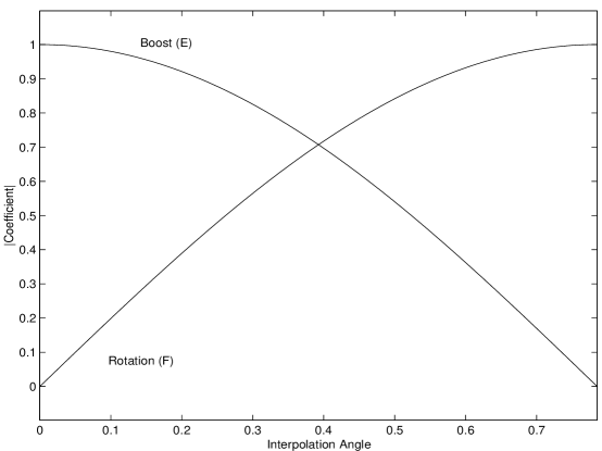
FIG. 1.: The smooth exchange of the roles of rotation and boost is displayed. The coefficients of rotation $F_{i}$ and boost $E_{i}$ in the dynamic generator ${\cal D}_{i}$ are plotted versus interpolation angle $\delta$.

We now construct the form for an arbitrary kinematic transformation on a fixed interpolation front. In general we have

$$T=e^{-i\beta_{3}{{K}^{3}}}e^{-i(\beta_{1}{{\cal K}_{1}}+\beta_{2}{{\cal K}_{2}})}$$ (34)

where $\beta_{1}$, $\beta_{2}$, and $\beta_{3}$ are free parameters. Under what conditions is $T$ kinematic? Use of the Baker-Hausdorff theorem reveals that

$$T^{\dagger}P^{+}T=P^{+}\cosh{\beta_{3}}+P_{-}\sinh{\beta_{3}}.$$ (35)

It follows that $x^{+}\rightarrow x^{+}\cosh{\beta_{3}}+x_{-}\sinh{\beta_{3}}$ under $T$. Note that $x^{+}\cosh{\beta_{3}}+x_{-}\sinh{\beta_{3}}=x^{+}\cosh{\beta_{3}}+({x^{+}}S-{x^{-}}C)\sinh{\beta_{3}}$. Now $T$ is kinematic if and only if the instant $x^{+}=0$ is invariant under $T$. This requires that $-{x^{-}}C\sinh{\beta_{3}}=0$. This can occur only if $C=0$ or $\beta_{3}=0$. Thus we find that $T$ is kinematic if $\delta=\frac{\pi}{4}$ or $\beta_{3}=0$. For $\delta\neq\frac{\pi}{4}$, then, $\beta_{3}=0$ and the kinematic transformation $T$ has two free parameters. On the light front, $\beta_{3}$ may take on any value and $T$ has three free parameters.

III SU(2) Spin Algebra and Dynamic Equations in an Arbitrary Interpolation Angle

In this section we construct the SU(2) spin algebra in an arbitrary interpolation angle. That is, we wish to construct operators ${\cal J}_{i}$ satisfying the criteria

$$[{\cal J}_{i},{\cal J}_{j}] = i\epsilon_{ijk}{\cal J}_{k},$$ (36)

$$[{\cal J}_{i},M] = 0,$$ (37)

where $M$ is the mass operator. We also require that $\vec{\cal J}$ commutes with every kinematic generator except $J_{3}$. We will see that such operators cannot be defined, in general, on the entire Hilbert space. Instead, we define a relevant subspace on which these operators are well- defined.

A Kinematic Subspace

Consider the set of momentum states that can be reached from rest by a kinematic transformation. We define this set of states to be the kinematic subspace for a fixed interpolating angle.

In general, kinematic transformations take the form given in Eq. (34), where $\beta_{3}=0$. We find that momentum operators transform under $T$ as follows:

$$T^{\dagger}{P_{-}}T = P_{-}\cos{\alpha}+\frac{\sin{\alpha}}{\alpha}C({\beta_{1}}P^{1}+{\beta_{2}}P^{2})$$ (38)

$$T^{\dagger}{P^{1}}T = P^{1}-\beta_{1}\frac{\sin{\alpha}}{\alpha}P_{-}+\frac{\cos{\alpha}-1}{{\alpha}^{2}}C{\beta_{1}}({\beta_{1}}P^{1}+{\beta_{2}}P^{2})$$ (39)

$$T^{\dagger}{P^{2}}T = P^{2}-\beta_{2}\frac{\sin{\alpha}}{\alpha}P_{-}+\frac{\cos{\alpha}-1}{{\alpha}^{2}}C{\beta_{2}}({\beta_{1}}P^{1}+{\beta_{2}}P^{2}),$$ (40)

where $\alpha=\sqrt{C({\beta_{1}}^{2}+{\beta_{2}}^{2})}$. This determines how momentum eigenvalues transform under $T$. At any interpolating angle, the rest state has momentum eigenvalues $P^{1}=P^{2}=0$ and $P_{-}=-MB$. It follows that any state which can be reached from rest must have a three-momentum of the form

$$(P_{-},P^{1},P^{2})=(-MB\cos{\alpha},\beta_{1}MB\frac{\sin{\alpha}}{\alpha},\beta_{2}MB\frac{\sin{\alpha}}{\alpha}).$$ (41)

Suppose we have a momentum state of the form given above. Then

$${\bf{P_{\perp}}}^{2}={P_{1}}^{2}+{P_{2}}^{2}=(MB\frac{\sin{\alpha}}{\alpha})^{2}({\beta_{1}}^{2}+{\beta_{2}}^{2})$$ (42)

and therefore

$${P_{-}}^{2}={M^{2}}{B^{2}}-C{\bf{P_{\perp}}}^{2}.$$ (43)

Conversely, any state satisfying (43) can be reached by a kinematic transformation. This condition also implies that $P^{+}=AM$.

In the equal-time case, $C=\cos{2\delta}=1$, $B=0$, and $P_{-}=P^{3}$. Thus $(P^{3})^{2}=-{\bf{\bf{P_{\perp}}}}^{2}$ and ${\bf P}^{2}=0$. The kinematic subspace in the equal-time case contains only the rest state. For a general interpolating angle, the kinematic subspace is a paraboloid in momentum space containing the origin. As we move to the light-front limit, $C=0$, $B=-\frac{1}{\sqrt{2}}$, and $P_{-}=P^{+}$. Therefore $P^{+}=\frac{M}{\sqrt{2}}$. In equal- time momentum space, this is the set of states on the paraboloid $P^{3}=-\frac{{\bf{P_{\perp}}}^{2}}{2M}$. If we allow $\beta_{3}\neq{0}$, however, the addition of longitudinal boost to the transformation $T$ allows us to move vertically off of this paraboloid, to a state with arbitrary longitudinal momentum. It follows that the kinematic subspace on the light-front is identical to the entire momentum space. This is a unique feature of $\delta=\frac{\pi}{4}$.

For $0<\delta<\frac{\pi}{4}$ and $P_{\perp}\neq{0}$, $|P_{-}|<-MB$ and we can invert Eq. (41) to find the parameters $\beta_{1}$ and $\beta_{2}$.

$$\alpha = \arccos{(-\frac{P_{-}}{MB})}$$ (44)

$$\beta_{1} = -\arccos{(-\frac{P_{-}}{MB})}\frac{P^{1}}{\sqrt{M^{2}{B^{2}}-{P_{-}}^{2}}}$$ (45)

$$= -\arcsin{(\frac{\sqrt{C}|{\bf{P_{\perp}}}|}{-MB})}\frac{P^{1}}{|{\bf{P_{\perp}}}|\sqrt{C}}$$ (46)

$$\beta_{2} = -\arccos{(-\frac{P_{-}}{MB})}\frac{P^{2}}{\sqrt{M^{2}{B^{2}}-{P_{-}}^{2}}}$$ (47)

$$= -\arcsin{(\frac{\sqrt{C}|{\bf{P_{\perp}}}|}{-MB})}\frac{P^{2}}{|{\bf{P_{\perp}}}|\sqrt{C}}.$$ (48)

B Construction of SU(2) Algebra

Following the procedure of Leutwyler and Stern [3], we now define the spin operators ${\cal J}_{i}$ through the use of a kinematic transformation. Within the kinematic subspace we define $T$ such that $T|n>=|p,n>$ . We define ${\cal J}$ within the subspace such that

$${\cal J}_{i}|p,n>=T{J_{i}}|n>.$$ (49)

That is, ${\cal J}_{i}=T{J_{i}}T^{\dagger}$ on all momentum eigenstates within the subspace. Then the operators satisfy the necessary SU(2) algebra:

$$[{\cal J}_{i},{\cal J}_{j}]|p,n> = T{J_{i}}{J_{j}}T^{\dagger}|p,n>-T{J_{j}}{J_{i}}T^{\dagger}|p,n>$$ (50)

$$= T[J_{i},J_{j}]T^{\dagger}|p,n>$$ (51)

$$= i\epsilon_{ijk}T{J_{k}}T^{\dagger}|p,n>$$ (52)

$$= i\epsilon_{ijk}{{\cal J}_{k}}|p,n>.$$ (53)

Note that the mass operator is defined by $M^{2}={P^{+}}{P_{+}}+{P^{-}}{P_{-}}-{\bf{P_{\perp}}}^{2}$. Some manipulation reveals that $[{\cal K}_{i},M^{2}]=0$, so $[T,M^{2}]=0$ and:

$$[{\cal J}_{i},M]|p,n> = T{J_{i}}T^{\dagger}M|p,n>-MT{J_{i}}T^{\dagger}|p,n>$$ (54)

$$= T{J_{i}}MT^{\dagger}|p,n>-TM{J_{i}}T^{\dagger}|p,n>$$ (55)

$$= T({J_{i}}M-M{J_{i}})T^{\dagger}|p,n>$$ (56)

$$= T({J_{i}}M-M{J_{i}})|n>$$ (57)

$$= T({J_{i}}{P^{0}}-{P^{0}}{J_{i}})|n>$$ (58)

$$= T[J_{i},P^{0}]|n>$$ (59)

$$= 0.$$ (60)

These operators then allow us to define simultaneous eigenstates of mass and spin.

Finally, each spin operator commutes with $T$ and $T^{\dagger}$:

$$[{\cal J}_{i},T^{\dagger}] = {\cal J}_{i}T^{\dagger}|p,n>-T^{\dagger}{\cal J}_{i}|p,n>$$ (61)

$$= {\cal J}_{i}|n>-T^{\dagger}TJ_{i}|n>$$ (62)

$$= J_{i}|n>-J_{i}|n>=0.$$ (63)

It follows that ${\cal J}_{i}$ commutes with the generators ${\cal K}_{1}$ and ${\cal K}_{2}$. Also, since the action of the spin operators is defined on momentum eigenstates, it is clear that simultaneous eigenstates of spin and momentum exist. Thus ${\cal J}_{i}$ commutes with all three components of the momentum operator. Thus, the spin operators commute with all generators of the stability group except $J_{3}$, as required.

For a given interpolation angle, we find the angular momentum operators in terms of the parameters $\beta_{1}$, $\beta_{2}$ to be:

$${\cal J}_{3} = {J_{3}}\cos{\alpha}+({\beta_{2}}{\cal K}_{1}-{\beta_{1}}{\cal K}_{2})\frac{\sin{\alpha}}{\alpha}$$ (64)

$${\cal J}_{1} = J_{1}+({\beta_{1}}A{J_{3}}-{\beta_{2}}B{K_{3}})\frac{\sin{\alpha}}{\alpha}$$ (65)

$$+ [{{\beta_{1}}^{2}}A{\cal K}_{2}-{{\beta_{2}}^{2}}BE_{2}-{\beta_{1}}{\beta_{2}}(A{\cal K}_{1}+BE_{1})]\frac{\cos{\alpha-1}}{\alpha^{2}}$$ (66)

$${\cal J}_{2} = J_{2}+({\beta_{2}}AJ_{3}+{\beta_{1}}BK_{3})\frac{\sin{\alpha}}{\alpha}$$ (67)

$$+ [-{\beta_{2}}^{2}A{\cal K}_{1}+{\beta_{1}}^{2}BE_{1}+{\beta_{1}}{\beta_{2}}(A{\cal K}_{2}+BE_{2})]\frac{\cos{\alpha}-1}{{\alpha}^{2}},$$ (68)

where

$$\alpha = \sqrt{C({\beta_{1}}^{2}+{\beta_{2}}^{2})}$$ (69)

$$A = C\cos{\delta}+S\sin{\delta}$$ (70)

$$B = C\sin{\delta}-S\cos{\delta}.$$ (71)

The action of each spin operator is determined by the three parameters $\delta,\beta_{1},\beta_{2}$. We first investigate the action of ${\cal J}$ by fixing $(\beta_{1},\beta_{2})$ and varying $\delta$. This traces a path in momentum space that begins at the rest state and ends on the surface $P^{3}=-\frac{{\bf{P_{\perp}}}^{2}}{2M}$, as in Fig 2. Here three distinct paths are visible, corresponding to different values for $(\beta_{1},\beta_{2})$. Along each path, the form of ${\cal J}$ is fixed and the coefficient of each generator depends continuously on interpolation angle. A path thus connects states from each kinematic subspace for which the equations of motion have a fixed form, and allows us to trace the fate of these equations as we move between interpolation angles.

In Fig 3, five paths are plotted in the plane $(P_{\perp},P^{3})$ with increasing $\beta_{1}=\beta_{2}$. Connecting the points on each path parameterized by the same value of $\delta$, we find a parabola that represents the kinematic subspace for the interpolation angle $\delta$. As $\delta$ increases, the parabola opens and becomes wider. On the light-front, the endpoints of these paths trace out the parabola $P^{3}=-\frac{{\bf{P_{\perp}}}^{2}}{2M}$.

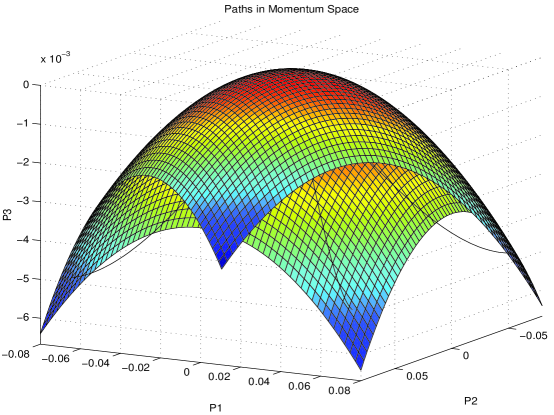
FIG. 2.: Three-dimensional plot of momentum states for fixed $\beta_{1},\beta_{2}$. Paths parameterized by $\delta$ begin at the rest state and end on a paraboloid at the light-front.

FIG. 3.: Momentum states for a fixed $\beta_{1}=\beta_{2}$ are plotted in momentum space. Each path begins at the rest state and cuts through a single point on the kinematic subspace.

We now investigate the action of ${\cal J}$ by fixing $\delta$. For a fixed interpolation angle, we have defined a kinematic subspace that is parameterized by $\beta_{1},\beta_{2}$. The action of the spin operators is defined everywhere on the subspace in terms of these two parameters. The representation of ${\cal J}$ at a fixed $\delta$ requires that we define $\beta_{1},\beta_{2}$ in terms of momentum operators. Using Eq. (44) we find

$${\cal J}_{3} = \frac{-1}{MB}(J_{3}P_{-}-{\cal K}_{1}P^{2}+{\cal K}_{2}P^{1})$$ (72)

$$\vec{\cal J}_{\perp} = {\bf{J_{\perp}}}+\frac{1}{MB}[{{\bf P}_{\perp}}A(J_{3}-\frac{\hat{\bf z}\cdot({{\bf P}_{\perp}}\times{{\vec{\cal K}}_{\perp})}}{MB-P_{-}})+(\hat{\bf z}\times{{\bf P}_{\perp}})B(K_{3}-\frac{{{\bf P}_{\perp}}\cdot{{\bf E}_{\perp}}}{MB-P_{-}})]$$ (73)

where we may write ${\bf J}_{\perp}=-\hat{\bf z}\times(A{\vec{\cal K}_{\perp}}+B{\vec{\cal D}_{\perp}})$. It is straightforward to show that the operator ${\cal J}_{3}$ commutes with every member of the stability group. We define ${\cal J}_{3}$ to be the helicity operator. Its simple form allows us to trace the fate of helicity states from equal-time to the light-front. The helicity operator can be written in terms of the Pauli-Lubanski operator $W_{\mu}=\frac{1}{2}{\epsilon}_{\mu\nu\alpha\beta}P^{\nu}M^{\alpha\beta}$ as ${\cal J}_{3}=\frac{-W^{+}}{MB}$.

It is important to note that helicity on any quantization front is in general frame-dependent. The above property, however, guarantees that helicities are identical in any two frames that are kinematically connected. On the light-front, for example, the Drell-Yan-West and Breit $(q^{+}=0)$ frames are kinematically connected. Thus, helicities must be identical in these two frames as demonstrated in Ref.[20].

For convenience, we present in Appendix B spin-1 and spin-1/2 representations for the helicity operator on an arbitrary interpolation front, as well as spin-1 polarization vectors and Dirac spinors.

C Limiting Cases

In Eq. (44), it is clear that problems arise when $\delta=0$, $\delta=\frac{\pi}{4}$, or $P_{\perp}=0$. We now investigate these problem points and discuss the equal-time and light-front limits. First, consider $\beta_{1},\beta_{2}$ as functions of momentum. Define $x=\frac{\sqrt{C}|\bf{\bf{P_{\perp}}}|}{-MB}$, so $0\leq{x}\leq{1}$. We expand $\beta_{1},\beta_{2}$ in powers of $x$. For $x<<1$ we keep the first term to find

$$\beta_{1}=-\frac{xP^{1}}{|{\bf{P_{\perp}}}|\sqrt{C}}=\frac{P^{1}}{MB}$$ (74)

$$\beta_{2}=-\frac{xP^{2}}{|{\bf{P_{\perp}}}|\sqrt{C}}=\frac{P^{2}}{MB}.$$ (75)

For $\delta\neq{0}$, we find $\beta_{i}\rightarrow{0}$ as $|P_{\perp}|\rightarrow{0}$. On the rest state, then, the action of ${\cal J}_{i}$ is identical to the action of the equal-time angular momentum $J_{i}$. It follows that $\beta_{1},\beta_{2}$ can be defined as continuous functions of momentum everywhere on the kinematic subspace.

Now let us consider the spin operators on the light-front. Recall that our construction of a general kinematic transformation $T$ required that $\beta_{3}=0$, which is necessary for $0\leq\delta<\frac{\pi}{4}$. In the special case of the light-front, however, the appearance of $K_{3}$ as a kinematic operator allows us to define a general kinematic transformation with $\beta_{3}\neq{0}$. Since the entire momentum space may be parameterized by $\beta_{1},\beta_{2},\beta_{3}$, the kinematic subspace becomes the entire momentum space. This is a unique and important feature of the light-front quantization $\delta=\frac{\pi}{4}$.

It follows that the action of the spin operators can be defined on any momentum eigenstate. The operators may be obtained as before, now using the kinematic transformation $T$ with $\beta_{3}=\ln\frac{P^{+}\sqrt{2}}{M}$, $\beta_{\perp{i}}=-\frac{P^{i}}{P^{+}}$ [3]. The resulting spin operators, valid for any momentum state, are given in terms of $\beta_{1},\beta_{2},\beta_{3}$:

$${\cal J}_{3} = J_{3}+{\beta_{1}}E_{2}-{\beta_{2}}E_{1}$$ (76)

$${\cal J}_{1} = \frac{1}{\sqrt{2}}[({\beta_{1}}J_{3}+{\beta_{2}}K_{3}+\frac{1}{2}({\beta_{1}}^{2}-{\beta_{2}}^{2})E_{2}+{\beta_{1}}{\beta_{2}}E_{1})e^{\beta_{3}}-{E_{2}}e^{-\beta_{3}}+{F_{2}}e^{\beta_{3}}]$$ (77)

$${\cal J}_{2} = \frac{1}{\sqrt{2}}[({\beta_{2}}J_{3}-{\beta_{1}}K_{3}+\frac{1}{2}({\beta_{2}}^{2}-{\beta_{1}}^{2})E_{2}-{\beta_{1}}{\beta_{2}}E_{1})e^{\beta_{3}}-{E_{2}}e^{-\beta_{3}}+{F_{2}}e^{\beta_{3}}].$$ (78)

The light-front spin operators are therefore

$${\cal J}_{3} = J_{3}+\frac{1}{P^{+}}({P^{2}}E_{1}-{P^{1}}E_{2})$$ (79)

$${\cal J}_{1} = \frac{1}{M}({P^{+}}F_{2}-{P^{-}}E_{2}-{P^{2}}K_{3}-{P^{1}}{\cal J}_{3})$$ (80)

$${\cal J}_{2} = \frac{1}{M}({P^{-}}E_{1}-{P^{+}}F_{1}+{P^{1}}K_{3}-{P^{2}}{\cal J}_{3}).$$ (81)

These are the spin operators presented in Appendix B of Ref.[36], where the operators $P^{+},E_{i},F_{i}$ do not contain our normalization factor of $\frac{1}{\sqrt{2}}$. It is important to compare this general light-front result with our interpolating spin operators.

Consider the light-front limit of the spin operators given in Eq. (64). In the light-front limit $C\rightarrow{0}$, and using the previous expansion we find that $\beta_{1}\rightarrow\frac{P^{1}}{MB}=-\frac{P^{1}\sqrt{2}}{M}$. The spin operators become

$${\cal J}_{3} = J_{3}+\frac{\sqrt{2}}{M}(P^{2}{E_{1}}-P^{1}{E_{2}})$$ (82)

$${\cal J}_{1} = \frac{1}{\sqrt{2}}({F_{2}}-{E_{2}})-\frac{1}{M}(P^{1}{J_{3}}+P^{2}{K_{3}})$$ (83)

$$- \frac{1}{{M^{2}}\sqrt{2}}[(-(P^{1})^{2}+(P^{2})^{2}){E_{2}}+2P^{1}{P^{2}}E_{1}]$$ (84)

$${\cal J}_{2} = \frac{1}{\sqrt{2}}({E_{1}}-{F_{1}})-\frac{1}{M}(P^{2}{J_{3}}-P^{1}{K_{3}})$$ (85)

$$- \frac{1}{{M^{2}}\sqrt{2}}[(-(P^{1})^{2}+(P^{2})^{2}){E_{1}}-2P^{1}{P^{2}}E_{2}].$$ (86)

Recall that in the light-front limit, ${\cal J}$ is defined on the subspace $\sqrt{2}{P^{+}}=M$. Within this subspace, Eq.(82) coincides with Eq.(79). It follows that our interpolating spin operators are consistent with the light-front spin operators within the subspace on which they are defined.

Now let us consider the equal-time limit. In the equal-time limit the kinematic subspace contains only the rest state, and $T$ becomes a rotation. Since any sequence of rotations leaves the rest state invariant, the parameters $\beta_{1},\beta_{2}$ may take on any value (see footnote 3). The spin operators become

$${\cal J}_{3} = J_{3}\cos{\alpha}+(-\beta_{2}{J_{2}}-\beta_{1}{J_{1}})\frac{\sin{\alpha}}{\alpha}$$ (87)

$${\cal J}_{1} = J_{1}+{\beta_{1}}{J_{3}}\frac{\sin{\alpha}}{\alpha}+({\beta_{1}}^{2}{J_{1}}+{\beta_{1}}{\beta_{2}}J_{2})\frac{\cos{\alpha}-1}{\alpha^{2}}$$ (88)

$${\cal J}_{2} = J_{2}+{\beta_{2}}{J_{3}}\frac{\sin{\alpha}}{\alpha}+({\beta_{2}}^{2}{J_{2}}+{\beta_{1}}{\beta_{2}}J_{1})\frac{\cos{\alpha}-1}{\alpha^{2}},$$ (89)

where $\alpha=\sqrt{{\beta_{1}}^{2}+{\beta_{2}}^{2}}$. If we set $\beta_{1}=0$, then

$${\cal J}_{3} = {J_{3}}\cos{\beta_{2}}-{J_{2}}\sin{\beta_{2}}$$ (90)

$${\cal J}_{1} = J_{1}$$ (91)

$${\cal J}_{2} = {J_{2}}\cos{\beta_{2}}+{J_{3}}\sin{\beta_{2}}.$$ (92)

These are rotated about the x-axis. Similarly if we set $\beta_{2}=0$, then

$${\cal J}_{3} = {J_{3}}\cos{\beta_{1}}-{J_{1}}\sin{\beta_{1}}$$ (93)

$${\cal J}_{1} = {J_{1}}\cos{\beta_{1}}+{J_{3}}\sin{\beta_{1}}$$ (94)

$${\cal J}_{2} = J_{2}.$$ (95)

These are rotated about the y-axis. Thus the spin operators are angular momentum operators $J_{1},J_{2},J_{3}$, about rotated axes, as we should expect. When we restrict $T$ to be the identity transformation, each $\beta_{i}=0$, and we recover the ordinary equal-time angular momentum operators.

IV Discussion and Conclusion

In this work, we constructed the Poincare algebra valid for any interpolation angle between the instant limit and the light-front limit. We find that the light-front limit $\delta=\frac{\pi}{4}$ is a special angle that adds a new kinematic operator $K_{3}$. The conversion of the dynamical operator between boost and rotation is quite smooth as shown in Fig.1. The general result of ${\cal J}$ in the instant limit agrees with the ordinary angular momentum ${\vec{J}}$ while it agrees with the LF ${\cal J}$ obtained by Leutwyler and Stern in the light-front limit with operation to the parabolic subspace shown in Fig.2. It is interesting to note that the subspace is limited to only the rest frame in the instant limit while it can expand to an arbitrary frame in the light-front limit. We have also presented the helicity operator in an arbitrary interpolation angle. Explicit verification for the correct helicity eigenvalues is summarized in the Appendix B. Since our results are model independent, they can play the role of testing any suggested hadron model. Our results indicate that the interpolation method preserving the orthogonal coordinate system is useful in tracing the fate of interesting results obtained by one form of Hamiltonian dynamics in the other end of interpolation angle. Applications to other nonperturbative analyses such as the BCS vacuum and the mass gap equation are under consideration.

A Poincaré Algebra on an Arbitrary Interpolating Front

$$[P^{-},P^{1}] = 0,$$ (A1)

$$[P^{-},P^{2}] = 0,$$ (A2)

$$[P^{-},P^{+}] = 0,$$ (A3)

$$[P^{-},E_{2}] = iP^{2}{S},$$ (A4)

$$[P^{-},E_{1}] = iP^{1}{S},$$ (A5)

$$[P^{-},J^{3}] = 0,$$ (A6)

$$[P^{-},F_{1}] = -iP^{1}{C},$$ (A7)

$$[P^{-},F_{2}] = -iP^{2}{C},$$ (A8)

$$[P^{-},K^{3}] = -iP_{+},$$ (A9)

$$[P^{1},P^{2}] = 0,$$ (A10)

$$[P^{1},P^{+}] = 0,$$ (A11)

$$[P^{1},E_{2}] = 0,$$ (A12)

$$[P^{1},E_{1}] = iP^{+}$$ (A13)

$$[P^{1},J^{3}] = -iP^{2}$$ (A14)

$$[P^{1},F_{1}] = iP^{-}$$ (A15)

$$[P^{1},F_{2}] = 0$$ (A16)

$$[P^{1},K^{3}] = 0$$ (A17)

$$[P^{2},P^{+}] = 0$$ (A18)

$$[P^{2},E_{2}] = iP^{+}$$ (A19)

$$[P^{2},E_{1}] = 0$$ (A20)

$$[P^{2},J^{3}] = iP^{1}$$ (A21)

$$[P^{2},F_{1}] = 0$$ (A22)

$$[P^{2},F_{2}] = iP^{-}$$ (A23)

$$[P^{2},K^{3}] = 0$$ (A24)

$$[P^{+},E_{2}] = iP^{2}{C}$$ (A25)

$$[P^{+},E_{1}] = iP^{1}{C}$$ (A26)

$$[P^{+},J^{3}] = 0$$ (A27)

$$[P^{+},F_{1}] = iP^{1}{S}$$ (A28)

$$[P^{+},F_{2}] = iP^{2}{S}$$ (A29)

$$[P^{+},K^{3}] = iP_{-}$$ (A30)

$$[E_{2},E_{1}] = iJ^{3}{C}$$ (A31)

$$[E_{2},J^{3}] = iE_{1}$$ (A32)

$$[E_{2},F_{1}] = iJ^{3}{S}$$ (A33)

$$[E_{2},F_{2}] = -iK^{3}$$ (A34)

$$[E_{2},K^{3}] = -i{\cal K}_{2}$$ (A35)

$$[E_{1},J^{3}] = -iE_{2}$$ (A36)

$$[E_{1},F_{1}] = -iK^{3}$$ (A37)

$$[E_{1},F_{2}] = -iJ^{3}{S}$$ (A38)

$$[E_{1},K^{3}] = -i{\cal K}^{1}$$ (A39)

$$[J^{3},F_{1}] = iF_{2}$$ (A40)

$$[J^{3},F_{2}] = -iF_{1}$$ (A41)

$$[J^{3},K^{3}] = 0$$ (A42)

$$[F_{1},F_{2}] = iJ^{3}{C}$$ (A43)

$$[F_{1},K^{3}] = i{\cal D}^{1}$$ (A44)

$$[F_{2},K^{3}] = i{\cal D}^{2}$$ (A45)

B Helicities on an Arbitrary Interpolation Front

The helicity operator may be represented for spin-1/2 states as follows:

$$[{\cal J}_{3}]_{\frac{1}{2}}=-\frac{1}{MB}\left(\begin{array}[]{cccc}P_{-}&AP_{L}&0&BP_{L}\\ AP_{R}&-P_{-}&-BP_{R}&0\\ 0&BP_{L}&P_{-}&AP_{L}\\ -BP_{R}&0&AP_{R}&-P_{-}\end{array}\right).\\$$ (B1)

Here $P_{R}=P^{1}+iP^{2}$ and $P_{L}=P^{1}-iP^{2}$. We found the spin-1/2 eigenstates of helicity by diagonalizing this matrix. These spinors are the solutions of the Dirac equation for an arbitrary interpolation angle:

$$u(p,+1) = -\frac{1}{\sqrt{B(MB-P_{-})}}\left(\begin{array}[]{c}MB-P_{-}\\ -AP_{R}\\ 0\\ BP_{R}\end{array}\right)$$ (B6)

$$u(p,-1) = -\frac{1}{\sqrt{B(MB-P_{-})}}\left(\begin{array}[]{c}AP_{L}\\ MB-P_{-}\\ BP_{L}\\ 0\end{array}\right).$$ (B11)

In addition, these spin-1/2 eigenstates are antiparticle solutions to the Dirac equation for an arbitrary angle:

$$v(p,+1) = \frac{1}{\sqrt{B(MB-P_{-})}}\left(\begin{array}[]{c}BP_{L}\\ 0\\ AP_{L}\\ MB-P_{-}\end{array}\right)$$ (B17)

$$v(p,-1) = -\frac{1}{\sqrt{B(MB-P_{-})}}\left(\begin{array}[]{c}0\\ BP_{R}\\ MB-P_{-}\\ -AP_{R}\end{array}\right).$$ (B22)

These spinors satisfy the following constraints:

$$({\not\!P}-m)u(p,\lambda) = 0$$ (B24)

$$({\not\!P}+m)v(p,\lambda) = 0$$ (B25)

$$\overline{u}(p,\lambda)u(p,\lambda^{\prime}) = 2m{\delta}_{\lambda\lambda^{\prime}}=-\overline{v}(p,\lambda^{\prime})v(p,\lambda)$$ (B26)

$${\sum_{\lambda}}u(p,\lambda)\overline{u}(p,\lambda) = {\not\!P}+M$$ (B27)

$${\sum_{\lambda}}v(p,\lambda)\overline{v}(p,\lambda) = {\not\!P}-M$$ (B28)

Similarly, for spin-1 states we have the representation

$$[{\cal J}_{3}]_{1}=\frac{i}{MB}\left(\begin{array}[]{cccc}0&-BP^{2}&BP^{1}&0\\ -BP^{2}&0&-P_{-}&AP^{2}\\ BP^{1}&P_{-}&0&-AP^{1}\\ 0&-AP^{2}&AP^{1}&0\end{array}\right).\\ \\$$ (B30)

We found the spin-1 eigenstates of helicity by diagonalizing this matrix. After proper normalization, we obtain the polarization vectors given by

$$\epsilon(p,0) = -\frac{A}{MB}(P_{+}-\frac{M^{2}}{P^{+}},P_{-},P^{1},P^{2})$$ (B31)

$$\epsilon(p,+1) = \frac{1}{\sqrt{2}MB}(S|P_{\perp}|,-C|P_{\perp}|,\frac{P_{-}P^{1}-iMBP^{2}}{|P_{\perp}|},\frac{P_{-}P^{2}+iMBP^{1}}{|P_{\perp}|})$$ (B32)

$$\epsilon(p,-1) = \frac{1}{\sqrt{2}MB}(S|P_{\perp}|,-C|P_{\perp}|,\frac{P_{-}P^{1}+iMBP^{2}}{|P_{\perp}|},\frac{P_{-}P^{2}-iMBP^{1}}{|P_{\perp}|}),$$ (B33)

where $\epsilon(p,\lambda)$ is written in the form $\epsilon(p,\lambda)=(\epsilon_{+},\epsilon_{-},\epsilon_{1},\epsilon_{2},)$. These polarization vectors satisfy the constraints

$$\epsilon(p,\lambda)\cdot{p} = 0$$ (B35)

$$\epsilon^{*}(p,\lambda)\cdot\epsilon(p,{\lambda}^{\prime}) = -\delta_{\lambda\lambda^{\prime}}$$ (B36)

$$\sum_{\lambda}\epsilon^{\mu}(p,\lambda)\epsilon^{\nu}(p,\lambda) = -g^{\mu\nu}+\frac{p^{\nu}p^{\mu}}{M^{2}}.$$ (B37)

It is also clear that the longitudinal polarization vector ${\epsilon}(p,0)$ is ”parallel” to the three-momentum $\bf P$, since $(\epsilon_{-},\epsilon_{1},\epsilon_{2})\sim{(P_{-},P_{1},P_{2})}$. This is a feature of both light-front and traditional equal-time definitions of longitudinal helicity $(h=0)$.

REFERENCES

- [1] S. Godfrey and N. Isgur, Phys. Rev. D 32, 189(1985).
- [2] P.A.M. Dirac, Rev. Mod. Phys. 21 , 392 (1949).
- [3] H.Leutwyler and J.Stern, Ann.Phys.(N.Y.)112,94(1978).
- [4] L.Ya.Glozman et al, Phys. Rev.D58, 094030(1998); R.F.Wagenbrunn et al, nucl-th/0010048 v2.
- [5] P.J. Steinhardt, Ann. Phys. 128 , 425 (1980).
- [6] S.Fubini, G. Furlan, Physics 1 , 229 (1965); S. Weinberg, Phys. Rev. 150 , 1313 (1966); J. Jersak and J. Stern, Nucl. Phys. B7 , 413 (1968); H. Leutwyler, in Springer Tracks in Modern Physics Vol. 50, ed. G. Höhler, (Berlin, 1969).
- [7] J.D. Bjorken, Phys. Rev. 179 , 1547 (1969); S.D. Drell, D. Levy, T.M. Yan, Phys. Rev. 187 , 2159 (1969), D1, 1035 (1970).
- [8] H.C. Pauli and S.J. Brodsky, Phys. Rev. D32 , 1993, 2001 (1985); S.J. Brodsky and H.C. Pauli, in ‘Recent Aspects of Quantum Fields’, eds. H. Mitter and H. Gausterer, Lecture Notes in Physics, Vol.396 (Springer, Berlin, 1991).
- [9] R.J. Perry, A.Harindranath, K.G. Wilson, Phys. Rev. Lett. 65 , 2959 (1990), Phys. Rev. D43 , 492, 4051 (1991); D. Mustaki, S. Pinsky, J. Shigemitsu and K. Wilson, Phys. Rev. D43 , 3411 (1991).
-
[10]
S.J. Brodsky, J.R. Hiller, and G. McCartor,
Phys. Rev. D 58, 025005 (1998);
J.R. Hiller, Pauli-Villars Regularization in a Discrete Light Cone Model, hep-ph/9807245. - [11] D.G.Robertson and G.McCartor, Z. Phys. C 53, 661 (1992); G.McCartor and D.G.Robertson, Z.Phys. C 53, 679 (1992).
- [12] S.J. Brodsky, H.C. Pauli, and S.S. Pinsky, Quantum Chromodynamics and Other Field Theories on the Light Cone, Phys. Rept. 301, 299 (1998).
- [13] E.Gubankova, C.-R.Ji and S.Cotanch, Phys. Rev D62, 125012 (2000).
- [14] L. Susskind and M. Burkardt, pp. 5 in Proceedings of the 4th International Workshop on Light-Front Quantization and Non-Perturbative Dynamics edited by S. D. Glazek (1994); K. G. Wilson and D. G. Rebertson, pp. 15 in the same proceedings.
- [15] W. Jaus, Phys. Rev. D44, 2851(1991).
- [16] H.-M. Choi and C.-R. Ji, Phys. Rev. D59,074015(1999); Phys. Rev. D56, 6010(1997).
- [17] H.-M. Choi and C.-R. Ji, Phys. Lett. B460,461(1999); Phys. Rev. D59,034001(1999).
-
[18]
S.D. Drell and T.M. Yan, Phys. Rev. Lett. 24 (1970) 181;
G. West, Phys. Rev. Lett. 24 (1970) -
[19]
C.-R. Ji, Acta Phys. Polon. B27, 3377-3380 (1996);
H.M. Choi and C.-R. Ji, Kaon Electroweak Form Factors in the Light-Front Quark Model, hep-ph/9807500;
H.-M. Choi and C.-R. Ji, Phys. Rev. D58, 071901 (1998);
H.-M. Choi and C.-R. Ji, Mixing Angles and Electromagnetic Properties of Ground State Pseudoscalar and Vector Meson Nonets in the Light Cone Quark Model, hep-ph/9711450. - [20] C.-R.Ji and C. Mitchell, Phys. Rev. D62,085020(2000).
- [21] M. V. Terent’ev, Yad. Fiz. 24, 207(1976) [ Sov.J. Nucl. Phys. 24, 106(1976)]; V. B. Berestetsky and M. V. Terent’ev, . 24, 1044(1976) [ 24, 547(1976)]; 25, 653(1977)[ 25, 347(1977)].
- [22] Z. Dziembowsky and L. Mankiewicz, Phys. Rev. Lett. 58, 2175(1987); Z. Dziembowsky, Phys. Rev.D37, 778(1988).
- [23] C.-R. Ji and S.R. Cotanch, Phys. Rev.D41, 2319(1990); C.-R. Ji, P.L. Chung and S.R. Cotanch, Phys. Rev.D45, 4214(1992).
- [24] H.-M. Choi and C.-R.Ji, Nucl. Phys.A618, 291(1997).
- [25] W. Jaus, Phys. Rev.D41, 3394(1990).
- [26] W. Jaus, Phys. Rev.D44, 2851(1991).
- [27] P.L. Chung, F. Coester, and W.N. Polyzou, Phys. Lett. B205, 545(1988).
- [28] H.-M. Choi and C.-R.Ji, Phys. Rev.D56, 6010(1997).
- [29] T.Huang,B.-Q. Ma,and Q.-X.Shen, Phys.Rev.D49, 1490(1994).
- [30] F.Schlumpf, Phys.Rev.D50, 6895(1994).
- [31] F. Cardarelli et al., Phys. Lett.B349, 393(1995); 359, 1(1995); 332, 1(1994).
- [32] H.-M.Choi and C.-R.Ji, Phys. Rev. D59, 074015 (1999).
- [33] S.J.Brodsky and H.-C.Pauli, in Recent Aspects of Quantum Fields, edited by H.Mitter and H.Gausterer, Lecture Notes in Physics, Vol.396(Springer Verlag,Berlin,1991).
- [34] C.-R.Ji and Y.Surya, Phys.Rev.D46, 3565 (1992).
- [35] C.-R. Ji and S.J. Rey, Phys. Rev.D53, 5815(1996).
- [36] B.D.Keister and W.N.Polyzou, in Advances in Nuclear Physics, edited by J.W.Negele and E.Vogt(Plenum,N.Y.,1991), Vol.20,p.225.