A Possibility to Measure $CP$-Violating Effects
in the Decay $K~{}\rightarrow~{}\mu\nu\gamma$

R.N. Rogalyov

Institute for High Energy Physics, Protvino, Russia.

It is argued that a precise measurement of the transverse component of the muon spin in the decay $K~{}\rightarrow~{}\mu\nu\gamma$ makes it possible to obtain more stringent limits on $CP$-violating parameters of the leptoquark, SUSY and left-right symmetric models. The results of the calculations of the $CP$-even transverse component of the muon spin in the decay $K~{}\rightarrow~{}\mu\nu\gamma$ due to the final-state electromagnetic interactions are presented. The weighted average of the transverse component of the muon spin comprises $\sim 2.3\times 10^{-4}$.

1. Introduction

The transverse component of the muon spin in the decay $K~{}\rightarrow~{}\mu\nu\gamma$ beyond the Standard Model is due to both the electromagnetic and CP- and T-violating interactions:

$$\xi=\xi_{\mbox{\tiny EM}}+\xi_{\mbox{\tiny odd}},$$ (1)

where $\xi_{\mbox{\tiny EM}}$ is the contribution of the electromagnetic Final-State Interactions (FSI) and $\xi_{\mbox{\tiny odd}}$ is the contribution of the $CP$-odd interactions.

Current limitations on the $CP$-violation parameters in various non-Standard models allow the transverse component of the muon spin in the decay $K~{}\rightarrow~{}\mu\nu\gamma$ to be rather large [1]: the left-right symmetric models based on the symmetry group $SU(2)_{L}\times SU(2)_{R}\times U(1)_{B-L}$ with one doublet $\Phi$ and two triplets $\Delta_{L,R}$ of Higgs bosons can give $\xi_{\mbox{\tiny odd}}\sim 3.5\times 10^{-3}$ [2], supersymmetric models—$\xi_{\mbox{\tiny odd}}\sim 5\times 10^{-3}$ [3], leptoquark models—$\xi_{\mbox{\tiny odd}}\sim 2.5\times 10^{-3}$ [4]. To extract the value of $\xi_{\mbox{\tiny odd}}$ from the experimental data, one should know the value of $\xi_{\mbox{\tiny EM}}$ exactly.

It has long been known that [5] the transverse polarization of the muon can be accounted for by the imaginary parts of the form factors parametrizing the expression for the amplitude of the decay. In this work, we compute the contribution of the electromagnetic FSI to the transverse component of the muon spin in the decay $K~{}\rightarrow~{}\mu\nu\gamma$ in the one-loop approximation (to be certain, we consider the decay $K^{+}\rightarrow\mu^{+}\nu\gamma$). Our calculations are performed in the framework of the Chiral Perturbation Theory (ChPT) [6].

It should be mentioned that some contributions to $\xi_{\mbox{\tiny EM}}$ were calculated in [8, 9]. In contrast to the mentioned calculations, we take into account a complete set of the diagrams contributing to the imaginary part of the decay amplitude in the leading order of the ChPT.

For the description of the decay $K^{+}(p_{K})\rightarrow\mu^{+}(k)\nu(k^{\prime})\gamma(q)$, we use the following variables: $M_{K}=494$ MeV and $m_{\ell}=106$ MeV are the kaon and muon masses;

$$x=\frac{2p_{K}\cdot q}{M_{K}^{2}};\ \ y=\frac{2p_{K}\cdot k}{M_{K}^{2}};\ \ \ \lambda=\frac{1-y+\rho}{x};\ \ \rho=\frac{m_{\ell}^{2}}{M_{K}^{2}};\ \ \gamma=\frac{F_{A}}{F_{V}};$$ (2)

$$\tau\;=\;(1-\lambda)x+\rho;\ \ \ \zeta=1-\lambda-\tau;\ \ F_{V}\;=\;{\sqrt{2}\,M_{K}\over 8\pi^{2}\,F};\ \ \ \ F_{A}\;=\;{4\sqrt{2}\,M_{K}\,\left(L_{9}+L_{10}\right)\over F};$$

$L_{9}=6.9\pm 0.7\times 10^{-3}$ and $L_{10}=-5.5\pm 0.7\times 10^{-3}$ are the parameters of the $O(p^{4})$ ChPT Lagrangian; and $F=93$ MeV. The relevant terms of the ChPT Lagrangian [6, 7] have the form

$$L_{\mbox{\tiny CHPT}}^{K\,\rightarrow\mu\nu\gamma}\!\!\!\!\! \!\!\!\!\!=FG_{\mbox{\tiny F}}V_{us}\partial_{\mu}K^{+}l_{\mu}^{-}-e\;\bar{\mu}\hat{A}\mu+ieA_{\mu}\partial_{\mu}K^{+}K^{-}+iG_{\mbox{\tiny F}}eV_{us}^{\ast}FK^{-}A_{\mu}l_{\mu}^{+}-$$

$$-\;{G_{\mbox{\tiny F}}eV_{us}^{\ast}\over F}\left({1\over 8\pi^{2}}\;\varepsilon^{\mu\nu\alpha\beta}\partial_{\mu}K^{+}\partial_{\alpha}A_{\nu}l_{\beta}^{-}-4\sqrt{2}\;iM_{\pi}(L_{9}+L_{10})\;\partial_{\mu}K^{+}l_{\nu}^{-}(\partial_{\mu}A_{\nu}-\partial_{\nu}A_{\mu})\right)-$$

$$-\ {\alpha\over 2\pi F}\varepsilon^{\mu\nu\alpha\beta}\partial_{\mu}A_{\nu}\partial_{\alpha}A_{\beta}\pi^{0}+{iG_{\mbox{\tiny F}}\over 2}V_{us}^{\ast}l_{\mu}^{-}\left(K^{+}\partial_{\mu}\pi^{0}\;-\;\pi^{0}\partial_{\mu}K^{+}\right),$$

where $G_{\mbox{\tiny F}}=1.17\times 10^{-5}$ GeV^-2 is the Fermi constant; $\alpha=e^{2}/(4\pi)=7.3\times 10^{-3}$, $e$ is the electron charge; $V_{us}=0.22$ is the element of the Cabibbo–Kobayashi–Maskawa matrix; $K^{+},\pi^{0},A,\nu\ \mbox{and}\ \mu$ are the fields of the $K^{+}$ meson, $\pi^{0}$ meson, photon, antineutrino, and muon, respectively; $l^{+}_{\beta}=\bar{\mu}\gamma_{\beta}(1-\gamma^{5})\nu$; $l^{-}_{\beta}=\bar{\nu}\gamma_{\beta}(1-\gamma^{5})\mu$.

2. Expression for Polarization of Muon
in Terms of Helicity Amplitudes

Experimentally, the transverse component of the muon spin can be defined as follows:

$$\xi={N_{+}-N_{-}\over 2\;(N_{+}+N_{-})},$$ (4)

where $N_{+}$($N_{-}$) is the number of the produced muons whose spin is directed along(against) a beforehand specified direction of polarization. We introduce vector $\vec{o}$ specifying such direction in the case under consideration. In the kaon rest frame, it is orthogonal to the vectors $\vec{q},\vec{k},$ and $\vec{k}^{\prime}$ (in this frame, these three vectors are linearly dependent):

$$\vec{\bf o}={2\over M_{K}^{2}\,x\sqrt{\lambda\zeta}}({\bf\vec{q}\times\vec{k}}),$$ (5)

a positive value of $\xi$ implies that the projection of spin of muon on vector $\vec{o}$ is positive: $\vec{s}\vec{o}>0$.

The respective 4-vector is defined as the unit vector orthogonal to the vectors $q,k,$ and $k^{\prime}$:

$$o^{\lambda}={2\over M_{K}^{3}\,x\sqrt{\lambda\zeta}}\;\varepsilon^{\mu\nu\rho\lambda}k^{\prime}_{\mu}k_{\nu}q_{\rho},$$ (6)

or, to put it differently,

$$o^{\mu}={\omega_{-}^{\mu}(k,k^{\prime})-\omega_{+}^{\mu}(k,k^{\prime})\over i\sqrt{2}},$$ (7)

where the vectors $\omega_{-}^{\mu}(k,k^{\prime})$ and $\omega_{+}^{\mu}(k,k^{\prime})$ are defined by the relations

$$\hat{\omega}_{+}(k,k^{\prime}) = -{\sqrt{2}\over 2M_{K}^{3}x\sqrt{\lambda\zeta}}\left(\hat{k}\hat{q}\hat{k}^{\prime}(1-\gamma^{5})+\hat{k}^{\prime}\hat{q}\hat{k}(1+\gamma^{5})-{2\rho x\lambda M_{K}^{2}\over 1-x-\rho}\hat{k}^{\prime}\right),$$ (8)

$$\hat{\omega}_{-}(k,k^{\prime}) = -{\sqrt{2}\over 2M_{K}^{3}x\sqrt{\lambda\zeta}}\left(\hat{k}\hat{q}\hat{k}^{\prime}(1+\gamma^{5})+\hat{k}^{\prime}\hat{q}\hat{k}(1-\gamma^{5})-{2\rho x\lambda M_{K}^{2}\over 1-x-\rho}\hat{k}^{\prime}\right).$$

The helicity amplitudes for the decay $K^{+}(p)\rightarrow\mu^{+}(k)\nu(k^{\prime})\gamma(q)$ are defined as follows:

$${\cal M}_{r\,s}=\langle\mu_{s}(k)\nu(k^{\prime})\gamma_{r}(q)|{\cal M}|K(p)\rangle$$ (9)

where $r=\pm$ is the helicity of the photon; $s=\pm$ is the helicity of the muon in the reference frame comoving with the center of mass of the muon and neutrino, and the amplitude ${\cal M}$ is defined by

$$S=1-(2\pi)^{4}i\delta(k+k^{\prime}+q-p){\cal M},$$

where $S$ is the scattering matrix in the respective channel.

The particles produced in the decay $K~{}\rightarrow~{}\mu\nu\gamma$ can be described by the wave function

$$|\Psi\rangle=S|K(p)\rangle \!\!\!\!=\!\!\!\! {1\over\Gamma}\int d\Phi\left({\cal M}_{-\,-}|\gamma_{-}(q)\mu_{-}(k)\nu(k^{\prime})\rangle\right.+{\cal M}_{-\,+}|\gamma_{-}(q)\mu_{+}(k)\nu(k^{\prime})\rangle$$

$$+{\cal M}_{+\,-}|\gamma_{+}(q)\mu_{-}(k)\nu(k^{\prime})\rangle\left.+{\cal M}_{+\,+}|\gamma_{+}(q)\mu_{+}(k)\nu(k^{\prime})\rangle\right),$$

where $\Gamma$ is the decay width, and the element of the phase space has the form

$$d\Phi={1\over(2\pi)^{5}}\delta(k+k^{\prime}+q-p){d^{3}{\bf k}\over 2k_{0}}{d^{3}{\bf k^{\prime}}\over 2k^{\prime}_{0}}{d^{3}{\bf q}\over 2q_{0}}.$$

The operator of spin $s_{\mu}$ acts on fermion states as follows:

$$s_{\mu}={W_{\mu}\over m}=-\;{\gamma_{\mu}\gamma^{5}\over 2}\hat{\varepsilon}_{0},$$ (11)

where $W_{\mu}$ is the Pauli–Lubanski vector and $\hat{\varepsilon}_{0}$ is the operator of the sign of energy. The average value of the transverse component of spin in the state $|\Psi\rangle$ is equal to $\langle\Psi|(-\;s_{\mu}\cdot o_{\mu})|\Psi\rangle$,

Since

$$\langle\mu_{-}(\vec{k})|s^{\nu}|\mu_{-}(\vec{k})\rangle = -{1\over 4m_{\ell}}\bar{v}(k,N)\gamma^{\nu}\gamma^{5}v(k,N)\ \ \ \ \ =\ \ {N^{\nu}\over 2},$$ (12)

$$\langle\mu_{-}(\vec{k})|s^{\nu}|\mu_{+}(\vec{k})\rangle = -{1\over 4m_{\ell}}\bar{v}(k,-N)\gamma^{\nu}\gamma^{5}v(k,N)\ \ =-\;{\omega_{-}^{\nu}\over\sqrt{2}},$$

$$\langle\mu_{+}(\vec{k})|s^{\nu}|\mu_{-}(\vec{k})\rangle = -{1\over 4m_{\ell}}\bar{v}(k,N)\gamma^{\nu}\gamma^{5}v(k,-N)\ \ =-\;{\omega_{+}^{\nu}\over\sqrt{2}},$$

$$\langle\mu_{+}(\vec{k})|s^{\nu}|\mu_{+}(\vec{k})\rangle = -{1\over 4m_{\ell}}\bar{v}(k,-N)\gamma^{\nu}\gamma^{5}v(k,-N)=-\;{N^{\nu}\over 2},$$

where spinor $v(k,N)$ describes the muon of momentum $k$ and vector of spin $N$,

$$N_{\nu}={(1-x-\rho)k_{\nu}-2\rho k^{\prime}_{\nu}\over m_{\ell}(1-x-\rho)},$$ (13)

the expectation value of the transverse component of the muon spin is determined by the relation

$$\xi={\Xi\over{\cal N}^{2}}\equiv{1\over{\cal N}^{2}}\left({\cal M}_{-\;-}^{\prime}{\cal M}_{-\;+}^{\prime\prime}-{\cal M}_{-\;+}^{\prime}{\cal M}_{-\;-}^{\prime\prime}\right.\left.+{\cal M}_{+\;-}^{\prime}{\cal M}_{+\;+}^{\prime\prime}-{\cal M}_{+\;+}^{\prime}{\cal M}_{+\;-}^{\prime\prime}\right),$$ (14)

where ${\cal N}$ is the normalization factor, ${\cal N}^{2}=\sum_{i,j=\pm}|{\cal M}_{i,j}|^{2}$; ${\cal M}_{r,s}={\cal M}_{r,s}^{\prime}+i{\cal M}_{r,s}^{\prime\prime}\ (r,s=\pm)$ (this formula is readily obtained by isolating an infinitesimal volume of the phase space of the particles produced in the decay and employing formula (2.)).

In the calculations of the helicity amplitudes we use the so called diagonal spin basis [10, 11, 12] formed by the vectors $\omega^{\mu}_{\pm}$ and light-like linear combinations of the vectors $k$ and $k^{\prime}$.

With the use of this basis, the helicity amplitude ${\cal M}_{r,s}$ can be represented in a manifestly covariant form

$${\cal M}_{r,s}=\bar{u}(k^{\prime}){\cal M}_{\alpha}(k,k^{\prime},q)\epsilon_{\alpha}(r)v(k,sN)=Tr{\cal M}_{\alpha}(k,k^{\prime},q)\epsilon_{\alpha}(r)v(k,sN)\bar{u}(k^{\prime}),$$ (15)

where the expression for ${\cal M}_{\alpha}(k,k^{\prime},q)$ is given by the Feynman diagrams, the polarization vectors of the photon are equal to

$$\epsilon_{\mu}(\pm)={\sqrt{2}\over 2M_{K}x\sqrt{\lambda\zeta}}\left(-x\lambda k_{\mu}+x(1-\lambda)k^{\prime}_{\mu}-(1-\rho-x)q_{\mu}\mp i\varepsilon_{kk^{\prime}q\mu}\right),$$ (16)

and the quantities $v(k,sN)\bar{u}(k^{\prime})$ can be brought in the form

$$v_{\mu}(k,-N)\bar{u}_{\nu}(k^{\prime}) = {(\hat{k}-m_{\ell})\hat{k}^{\prime}\over 2M_{K}\sqrt{1-x-\rho}}(1+\gamma^{5}),$$ (17)

$$v_{\mu}(k,N)\bar{u}_{\nu}(k^{\prime})\ = {M_{K}^{2}(1-x-\rho)-m_{\ell}\hat{k}^{\prime}\over 2M_{K}\sqrt{1-x-\rho}}\;\hat{\omega}_{-}(1+\gamma^{5}).$$

The leading contribution to the real part of the decay amplitude is given by the tree diagrams corresponding to the Lagrangian (1.) [7] (see Fig. 1). The helicity amplitudes for the decay $K^{+}\rightarrow\mu^{+}\nu\gamma$ in the tree approximation have the form

$${\cal M}_{-\;-} = 2\,iG_{\mbox{\tiny F}}eV_{us}^{\ast}m_{\ell}x\sqrt{\lambda\zeta\over 1-x-\rho}\left({\sqrt{2}F(1-\rho)\over x^{2}(1-\lambda)}-\right.\left.M_{K}{F_{V}-F_{A}\over 2}\right),$$ (18)

$${\cal M}_{-\;+} = -2\,iG_{\mbox{\tiny F}}eV_{us}^{\ast}{x\lambda\over\sqrt{1-x-\rho}}\left(m_{\ell}F{\sqrt{2\rho}\over x(1-\lambda)}-{F_{V}-F_{A}\over 2}M_{K}^{2}(1-x)\right),$$

$${\cal M}_{+\;-} = 2\,iG_{\mbox{\tiny F}}eV_{us}^{\ast}m_{\ell}x\sqrt{\lambda\zeta\over 1-x-\rho}\left(F{\sqrt{2}(1-x-\rho)\over x^{2}(1-\lambda)}\right.\left.+{F_{V}+F_{A}\over 2}M_{K}\right),$$

$${\cal M}_{+\;+} = iG_{\mbox{\tiny F}}eV_{us}^{\ast}{(F_{V}+F_{A})x\over\sqrt{1-x-\rho}}M^{2}_{K}\zeta,$$

where the first index in the left-hand side denotes the polarization of the photon and the second—the polarization of the muon in the reference frame comoving with the center of mass of the lepton pair. The calculation of the imaginary parts of the helicity amplitudes is considered in the following Section.

The differential probability for the decay is determined by the matrix element squared

$$\sum_{polariz.}|{\cal M}|^{2}=|G_{\mbox{\tiny F}}eV_{us}^{\ast}|^{2}\;\left(m_{\ell}^{2}F^{2}\,IB\,+\,{(F_{V}+F_{A})^{2}\over 2M^{2}_{K}}SD_{+}+{(F_{V}-F_{A})^{2}\over 2M^{2}_{K}}SD_{-}\right.+$$ (19)

$$+\left.m_{\ell}F\,{F_{V}+F_{A}\over\sqrt{2}M_{K}}INT_{+}+m_{\ell}F\,{F_{V}-F_{A}\over\sqrt{2}M_{K}}INT_{-}\right),$$

where

$$IB = {8\lambda\over x^{2}(1-\lambda)}\ \left(x^{2}+2(1-x)(1-\rho)-{2\rho(1-\rho)\over 1-\lambda}\right),$$ (20)

$$SD_{+} = 2M^{6}_{K}x^{2}(1-\lambda)\zeta,$$

$$SD_{-} = 2M^{6}_{K}x^{2}\lambda\left((1-x)\lambda+\rho\right),$$

$$INT_{+} = {8M^{2}_{K}m_{\ell}\lambda\over 1-\lambda}\zeta,$$

$$INT_{-} = -\;{8M_{K}^{2}m_{\ell}\lambda\over 1-\lambda}\left(1-\lambda+\lambda x-\rho\right).$$

3. Contribution of FSI to Imaginary Part
of Decay Amplitude

The imaginary part of the amplitude for the decay $K~{}\rightarrow~{}\mu\nu\gamma$ in the leading order of the perturbation theory is described by the diagrams in Fig. 2. We take into account the diagrams in Figs. 2$g,h$ omitted by the authors of [8] in spite of the fact that they are of the same order of magnitude.

We employ the Cutkosky rules [13] to replace the propagators with the $\delta$ functions. Thus we obtain the expression for the imaginary part of the amplitude in terms of the integrals:

$${\cal M}^{\prime\prime}_{i}=-\,{\alpha F\over 2\pi}G_{\mbox{\tiny F}}eV_{us}^{\ast}\int dr{\Delta\over N_{i}(r\cdot q,r\cdot k)}\bar{u}(k^{\prime})(1+\gamma^{5})T_{i}(r,k,k^{\prime},q,\epsilon)v(k),$$ (21)

where $N_{i}$ is the product of the remaining propagators in the respective diagram and $T_{i}$ are the respective tensor structures (label $i$ specifies the diagram in Fig. 2, $i=$a$\div$i); in the case of the diagrams in Figs. 2$a$–$h$, $\Delta=\delta(r^{2}-m_{\ell}^{2})\delta\left((k+q-r)^{2}\right)$ whereas, for the diagram in Fig. 2$i$ $\Delta=\delta((r+q)^{2}-M_{\pi}^{2})\delta((k-r)^{2}-m_{\ell}^{2})$ ($M_{\pi}=135$ MeV — is the mass of the $\pi^{0}$ meson).

The computations of the diagrams in Fig. 2 are made with the REDUCE package. These diagrams are calculated exactly, no approximation is used.

The calculated imaginary part of the amplitude of the decay $K~{}\rightarrow~{}\mu\nu\gamma$ takes the form

$${\cal M^{\prime\prime}}=\;-\;{G_{\mbox{\tiny F}}eV_{us}^{\ast}\over 4\pi}\bar{u}_{\nu}(k^{\prime})(1+\gamma^{5})\left({\cal M}^{IB}+{\cal M}^{SD}+{\cal M}^{(\pi)}\right)v_{\mu}(k),$$ (22)

where

$${\cal M}^{IB}={2\pi\alpha F\over M_{K}^{2}}\sum_{n=1}^{4}c_{n}^{IB}{\cal E}_{n}$$

— is the contribution of the diagrams in Figs. 2$a$, 2$b$, 2$c$, 2$d$, 2$g$, 2$h$;

$${\cal M}^{SD}={\pi\sqrt{2}\alpha\over M_{K}}\sum_{n=1}^{4}(-F_{A}c^{A}_{n}+F_{V}c^{V}_{n}){\cal E}_{n}$$

— is the contribution of the diagrams in Figs. 2$e$ and 2$f$ and

$${\cal M}^{(\pi)}={\alpha\over 4\pi F}\left(c^{(\pi)}_{2}{\cal E}_{2}+c^{(\pi)}_{4}{\cal E}_{4}\right)$$

— is the contribution of the diagram in Fig. 2$i$. Tensor structures ${\cal E}_{i}$ have the form

$${\cal E}_{1} = M_{K}^{2}m_{\ell}x\left[(1-\lambda)k^{\prime}\cdot\epsilon-\lambda k\cdot\epsilon\right],$$ (23)

$${\cal E}_{2} = M_{K}^{2}\left[k\cdot\epsilon\hat{q}-\frac{M_{K}^{2}}{2}x(1-\lambda)\hat{\epsilon}\right],$$

$${\cal E}_{3} = M_{K}^{2}\left[k^{\prime}\cdot\epsilon\hat{q}-\frac{M_{K}^{2}}{2}x\lambda\hat{\epsilon}\right],$$

$${\cal E}_{4} = M_{K}^{2}m_{\ell}\hat{q}\hat{\alpha},$$

and the coefficients in the above expressions are given by

$$c_{1}^{IB} = -\;{4\over(1-\lambda)x}(G_{3}-(1+\tau)G_{2}+\rho(F_{1}-F_{2})),$$ (24)

$$c_{2}^{IB} = {4\rho\over(1-\lambda)x}(2G_{1}+(1+\tau)G_{2}-(1-\tau)G_{3}-(\tau+\rho)F_{1})+2F_{5}\rho,$$

$$c_{3}^{IB} = 4\rho(-F_{2}-G_{4}),$$

$$c_{4}^{IB} = {2\lambda\over(1-\lambda)}(G_{3}-G_{2}-\rho F_{2})-2(G_{2}+2G_{1}-F_{1})$$

$$+{4-x(1-\lambda)\over(1-\lambda)x}(2G_{1}+G_{2}-(1-\tau)G_{3}-\rho F_{3})+{2\over(1-\lambda)}(-\tau F_{1}+\rho F_{3})-F_{4}+F_{5}\rho,$$

$$c^{V}_{1} = ({1\over 3}x(1-\lambda)-2\tau)F_{5}+(\tau+\rho)F_{6},$$ (25)

$$c^{V}_{2} = {1\over 3}(\tau(1+5\tau-14\rho)-\rho(1-3\rho+x\lambda))F_{5}+\rho(\lambda x+2\rho)F_{6}+(1-\tau)F_{7}-{(1+\lambda)\over(1-\lambda)}F_{8},$$

$$c^{V}_{3} = -x(1-\lambda)(\tau+{\rho\over 3})F_{5}-\tau F_{7}+F_{8},$$

$$c^{V}_{4} = {1\over 2}(x(x(1-\lambda)^{2}+\tau(3-2\lambda))F_{5}+x(1-x-\lambda+\lambda x+\rho(3\lambda-4))F_{6}+(1-\tau)F_{7}),$$

$$c^{A}_{1} = c^{V}_{1},$$

$$c^{A}_{2} = c^{V}_{2}+2(-({5x^{2}(1-\lambda)^{2}\over 3}-\rho^{2})F_{5}+\rho(x-x\lambda-\rho)F_{6}+\tau F_{7}),$$

$$c^{A}_{3} = c^{V}_{3},$$

$$c^{A}_{4} = c^{V}_{4}+{1\over 2}(-x(1-\lambda)(\tau+2x(1-\lambda))F_{5}+4\rho x(1-\lambda)F_{6}+3\tau F_{7}),$$

$$c^{(\pi)}_{2} = {1\over 4M_{K}^{2}\,x^{2}(1-\lambda)^{2}}\theta\left(x-{\kappa+\sqrt{2\kappa\rho}\over 1-\lambda}\right)\;\left({2\kappa^{2}\rho\over x(1-\lambda)}S_{4}+\right.$$

$$+((x^{2}(1-\lambda)^{2}-\rho\kappa)({x(1-\lambda)\over\tau}+2)\left.+x^{2}(1-\lambda)^{2}){S\over\tau}\right),$$

$$c^{(\pi)}_{4} = {1\over 4M_{K}^{2}\,x^{2}(1-\lambda)^{2}}\theta\left(x-{\kappa+\sqrt{2\kappa\rho}\over 1-\lambda}\right)\;\left({\kappa^{2}(2\tau+\rho)\over x(1-\lambda)}S_{4}+\right.$$

$$+((x^{2}(1-\lambda)^{2}-\rho\kappa)({x(1-\lambda)\over\tau}+3)\left.-3\kappa(x(1-\lambda)+\tau)){S\over 2\tau}\right),$$

where

$$S=\sqrt{((1-\lambda)x-\kappa)^{2}-4\kappa\rho}\,\ \ \ \ \ \ \kappa={M_{\pi}^{2}\over M_{K}^{2}};$$ (27)

$\theta$ function in formula (3.) isolates the kinematic domain in which the imaginary part of the diagram in Fig. 2$i$ does not vanish;

$$S_{1} = \ln\left[1+{(1-\lambda)x\over\rho}\right],$$ (28)

$$S_{2} = \ln[\rho],$$

$$S_{3} = \ln\left[{1-\lambda x+\rho+\sqrt{R}\over 1-\lambda x+\rho-\sqrt{R}}\right],$$

$$S_{4} = \ln\left[{(1-\lambda)x(\kappa-(1-\lambda)x+S)+2\kappa\rho\over(1-\lambda)x(\kappa-(1-\lambda)x-S)+2\kappa\rho}\right],$$

$$R = (1-\lambda x+\rho)^{2}-4\rho,$$

$$F_{0} = {1\over 2M_{K}^{2}(1-\tau)x}\left(1-{\rho\over\tau}+{1-\rho\over 1-\tau}(S_{1}+S_{2})\right),$$ (29)

$$F_{1} = {1\over 4M_{K}^{2}x\zeta}\left(-2S_{1}-S_{2}+{1-\lambda x+\rho\over\sqrt{R}}S_{3}-{2\rho\over(1-\lambda)\sqrt{R}}S_{3}\right),$$

$$F_{2} = {1\over 4M_{K}^{2}\lambda x\zeta}\left({2\lambda\over 1-\tau}S_{1}-{\zeta-\lambda\over 1-\tau}S_{2}-{\zeta-\lambda+x\over\sqrt{R}}S_{3}\right),$$

$$F_{3} = {1\over 2M_{K}^{2}(1-\lambda)x\sqrt{R}}S_{3},$$

$$F_{4} = {1\over M_{K}^{2}(1-\lambda)^{2}x^{2}}((1-\lambda)x-\rho S_{1}),$$

$$F_{5} = {1\over 2M_{K}^{2}\tau^{2}},$$

$$F_{6} = {1\over M_{K}^{2}x(1-\lambda)}\left({S_{1}\over x(1-\lambda)}-{1\over\tau}\right),$$

$$F_{7} = {-x(1-\lambda)\over 6M_{K}^{2}\tau^{3}}(x-x\lambda+3\rho),$$

$$F_{8} = {\rho\over M_{K}^{2}x(1-\lambda)}\left({x-x\lambda+2\rho\over x(1-\lambda)}S_{1}-2\right),$$

$$G_{1} = {1\over 8M_{K}^{2}\lambda x\zeta}\left({2\lambda\over(1-\tau)}(\rho-\tau^{2})S_{1}+\right.$$

$$\left.+{1-\lambda\over 1-\tau}(1-2\rho-x-\tau x+\tau^{2})S_{2}+(1-\lambda)\sqrt{R}S_{3}\right),$$

$$G_{2} = {1\over\zeta}(-\lambda\rho F_{3}+2\lambda G_{1}-(1-\tau)F_{0}),$$

$$G_{3} = {1\over\zeta}(-\rho F_{3}+2G_{1}-F_{0}),$$

$$G_{4} = {1\over\lambda x}(-2G_{1}+\tau(G_{2}-F_{1})+\rho(F_{3}-F_{1})).$$

Substituting the expressions (22)–(3.) in formula (14), we represent the transverse muon polarization in the form

$$\xi_{\mbox{\tiny EM}}=-\;\frac{\sum_{n=1}^{4}c_{n}Y_{n}}{\sum_{r,s=\pm}|{\cal M}_{r,s}|^{2}},$$ (31)

where

$$c_{n}={\alpha\over 4}\;{G_{\mbox{\tiny F}}eV_{us}^{\ast}\over M_{K}^{2}}\left(2Fc_{n}^{IB}+\sqrt{2}\,M_{K}(c_{n}^{V}F_{V}-c_{n}^{A}F_{A})+{M_{K}^{2}\over 4\pi^{2}F}c_{n}^{(\pi)}\right),$$ (32)

$$Y_{n} = \bar{u}(k^{\prime})(1+\gamma^{5}){\cal E}_{n}^{\alpha}\left(\epsilon_{\alpha}^{-}(q)({\cal M}^{\prime}_{-,-}v_{+}(k)-{\cal M}^{\prime}_{-,+}v_{-}(k))+\right.$$

$$\hskip 56.9055pt\left.+\epsilon_{\alpha}^{+}(q)({\cal M}^{\prime}_{+,-}v_{+}(k)-{\cal M}^{\prime}_{+,+}v_{-}(k))\right),$$

$v_{\pm}(k)=v(k,\pm N)$. Since the imaginary parts of the amplitudes under consideration are much less than the respective real parts (${\cal M}^{\prime\prime}_{r,s}<\!\!\!<{\cal M}^{\prime}_{r,s}$), the denominator of the expression (31) is determined by the equation (19). The coefficients $c_{n}^{IB},c_{n}^{V},c_{n}^{A},c_{2}^{(\pi)},$ and $c_{4}^{(\pi)}$ are given in formulas (24)–(3.); $c_{1}^{(\pi)}=c_{1}^{(\pi)}=0$; and

$$Y_{1} = {G_{\mbox{\tiny F}}eV_{us}^{\ast}m_{\ell}M_{K}^{3}\sqrt{2\lambda\zeta}\over 1-\lambda}\left(M_{K}x^{2}(1-\lambda)\left((F_{V}-F_{A})(1-x-\rho)+\right.\right.$$

$$+\left.\left.2\,F_{A}\zeta\right)-2\sqrt{2}F\rho\lambda\right),$$

$$Y_{2} = {G_{\mbox{\tiny F}}eV_{us}^{\ast}m_{\ell}M_{K}^{3}\sqrt{2\lambda\zeta}\over 1-\lambda}\;\left(M_{K}x^{2}\lambda(1-\lambda)(F_{V}-F_{A})+2\sqrt{2}F(-\zeta+\lambda\rho)\right),$$

$$Y_{3} = {G_{\mbox{\tiny F}}eV_{us}^{\ast}m_{\ell}M_{K}^{3}\sqrt{2\lambda\zeta}\over 1-\lambda}\left(M_{K}x^{2}\lambda(1-\lambda)(F_{A}-F_{V})+2\sqrt{2}F\lambda(1-\rho)\right),$$

$$Y_{4} = {G_{\mbox{\tiny F}}eV_{us}^{\ast}m_{\ell}M_{K}^{3}\sqrt{2\lambda\zeta}\over 1-\lambda}\left(2M_{K}x^{2}\lambda(1-\lambda)(F_{A}-F_{V})-4\sqrt{2}F\lambda\rho\right).$$

4. Discussion of Results and Conclusion

The transverse component of the muon spin in the decay $K~{}\rightarrow~{}\mu\nu\gamma$ is plotted in Figs. 3 and 4 as a function of the kinematic variables $x$ and $y$. As is seen, it varies through the range $(0\div 7)\times 10^{-4}$ and the the weighted average is equal to (the notation see in formula (14)

$$\langle\xi_{\mbox{\tiny EM}}\rangle={\int_{x_{min}}dx\int dy\Xi\over\int_{x_{min}}dx\int dy{\cal N}^{2}}\simeq 2.3\times 10^{-4},$$ (35)

where the lower limit of the integration with respect to $x$, $x_{min}=0.1$, corresponds to the cutoff energy of the photon $\simeq 25MeV$. The accuracy of the result $\simeq 20\%$ is determined by the accuracy of the ChPT in order $O(p^{4})$ at these energies. Note that $\xi_{\mbox{\tiny EM}}$ is negative in sign over all Dalitz plot (positive direction is given by the vector $\vec{o}$ introduced in Section 2.)

The values of the parameters $F_{V}$ and $F_{A}$ used in our plots are: $F_{A}=0.042$ and $F_{V}=0.095$; these values predicted by CHPT coincide with those used in [8, 17].

The transverse polarization (which is twice the muon spin) agrees well with the results presented recently [17] and disagree with [8] and [9]. The point is that the authors of [8, 9] took into account only a part of the diagrams contributing to the transverse polarization of the muon. Our results show that the diagram estimated in [9] does not give a leading contribution to the imaginary part of the amplitude and the maximum value of the transverse polarization of the muon is overestimated in [8] by an order of magnitude. However, it should be emphasized that our results sustantiate the conclusion made in [9]: ”An experimental evidence of $P_{T}=2\xi$ at the level of $10^{-3}$ would be a clear signal of physics beyond the SM,” — in spite of the fact that the analysis performed in [9] is incomplete. Our results contradict to the conclusion of [8].

Thus an observation of the transverse spin of the muon of the order $10^{-3}$ in the experiments [14, 15, 16] would signal $CP$ and $T$ violation because the background $CP$-even effect does not exceed $7\times 10^{-4}$ and its average value is not over $3\times 10^{-4}$. Experiments of this sort can be a good tool for testing the above-mentioned non-Standard models.

Acknowledgment:  I am grateful to A.E. Chalov, V.V. Braguta, and A.A. Likhoded for the interest in the study.

   

Figure 1: Diagrams describing the decay $K~{}\rightarrow~{}\mu\nu\gamma$ in the tree approximation.

   

Figure 2: Diagrams giving a contribution to the imaginary part of the amplitude of the decay $K~{}\rightarrow~{}\mu\nu\gamma$.

   

Figure 3: Contour plot for the transverse spin $\xi_{\mbox{\tiny EM}}$. Curve A: $\xi_{\mbox{\tiny EM}}=\,2.5\times 10^{-4}$, curve B: $\xi_{\mbox{\tiny EM}}=\,5\times 10^{-4}$.

   

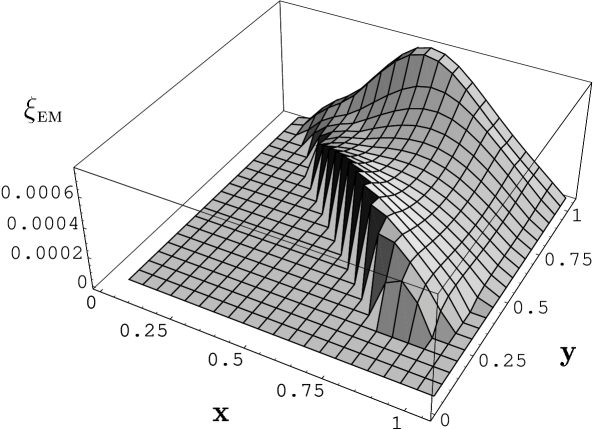
Figure 4: The electromagnetic contribution to the transverse component of the muon spin over the Dalitz plot for the decay $K~{}\rightarrow~{}\mu\nu\gamma$.