A MINIMAL MODEL WITH LARGE EXTRA DIMENSIONS TO FIT THE NEUTRINO DATA

The existence of large extra dimensions enables to explain very simply the various neutrino suppression data. The flavour neutrinos, confined on the brane, are coupled to a ”bulk” neutrino state, which is seen as an infinite tower of Kaluza-Klein states from the 4-dimensional point of view. The oscillation of flavour neutrinos into these states can lead to a global and sizable energy-independent suppression at large distances, which can be related to the solar neutrino puzzle. $\!{}^{{\bf?}}$

1 Introduction

The possibility of ”large extra dimensions”, i.e. with (at least) one compactification radius close to the current validity limit of Newton’s law of gravitation ($\sim$ 1mm), raises considerable interest. One reason is that it could solve the ”so-called” hierarchy problem $\!{}^{{\bf?}}$ by providing us with a new fundamental energy scale $M_{*}$ around 1 TeV. The discrepancy between the apparent huge value of the Planck scale and the weak scale then results from the fact that extra dimensions remain ”hidden” at low energies for all interactions except gravitation. From the relation

$$M^{2}_{Planck}=V_{n}\cdot M^{n+2}_{*}$$

we see that at least 2 extra dimensions are needed ($n\geq 2$) to avoid deviations from Newton’s law.

Another reason is that it can bring some new physics just ”around the corner”, at energies as low as 1 TeV. In particular, neutrino physics is a ideal area to study new theories. While particles belonging to the Standard Model (SM) are required to be confined on the usual four dimensional spacetime (the 3-brane with thickness $\sim 1~{}TeV^{-1}$), sterile neutrinos, which do not experience any of the gauge interactions, can propagate in the 4+n dimensional spacetime as well as gravitons, and turn to be an efficient tool to probe the ”bulk” of space.

From the four dimensional point of view, bulk neutrinos appear as an infinite tower of states, called the Kaluza-Klein states $\!{}^{{\bf?}}$, as a result of the compactification of the extra dimensions. When coupled to SM flavour neutrinos, unconventional patterns of neutrino masses and mixings arise. Recent works $\!{}^{{\bf?},{\bf?},{\bf?},{\bf?}}$ have shown that it is, at least partially, possible to accommodate experimental constraints on neutrinos within this setup.

A common feature of these solutions is that the solar $\nu_{e}$ depletion is explained using a small mixing between flavour and bulk neutrinos, which is enhanced in the sun by matter effects, the so-called Mikheyev-Smirnov-Wolfenstein (MSW)mechanism. These solutions are analogous to the classical Small Mixing Angle oscillation solution (SMA), and are strongly energy-dependent. However, recent analysis of SuperKamiokande (SK) data disfavours this kind of solutions, as no spectral distortion, nor seasonal effect, nor day-night effect are observed. Therefore, a global 40-60% suppression , which is energy and distance independent, is perfectly compatible with the observed deficit.

Using the setup of large extra dimensions, we explore this possibility in details. We also require that no MSW effects are present, otherwise, inescapable resonances in the sun could kill the final large distance survival probability. Finally, we try to accommodate other experimental constraints on neutrinos, including the depletion of atmospheric $\nu_{\mu}$, the $\overline{\nu}_{e}$ no disappearance at Chooz, the $\nu_{\mu}$ disappearance at K2K, $\overline{\nu}_{e}$ no appearance at Karmen and the LSND signal .

2 The 1-flavour model.

As a first attempt, we will investigate a toy model in which only 1 flavour neutrino $\nu_{1}$ (either of $\nu_{e}$, $\nu_{\mu}$, $\nu_{\tau}$) is coupled to one massless bulk fermion $\Psi$ through a Yukawa coupling constant $\lambda$. Moreover, we consider that only one extra dimension, taken as a circle of radius $R$, is relevant from the four dimensional point of view (i.e. all other extra dimensions are assumed to be much smaller).

The 5D action used is the following $\!{}^{{\bf?},{\bf?}}$ :

$$S=\int d^{4}x\,dy\;\overline{\Psi}i\Gamma_{A}\partial^{A}\Psi+\int d^{4}x\{\overline{\nu}_{1}i\gamma_{\mu}\partial^{\mu}\nu_{1}+\lambda\overline{\nu}_{1}\Psi(x^{\mu},y=0)H(x^{\mu})+h.c.\}$$ (1)

where $A=0,...,4$ and $x^{4}=y$ is the extra dimension. The Yukawa coupling between the usual Higgs scalar $H$, the weak eigenstate neutrino $\nu_{1}$ and the bulk fermion only operates at $y=0$, i.e. on the 3-brane.

Expanding the bulk fermion into Fourier modes (or Kaluza-Klein states),

$$\Psi(x^{\mu},y)=\sum_{n=-\infty}^{+\infty}\frac{1}{\sqrt{2\pi R}}\psi_{n}(x^{\mu})e^{iny/R}$$

and replacing $H$ by its vacuum expectation value $v$, one ends up with an infinite mass matrix with eigenvalues $\frac{\lambda_{n}}{R}$ given by the characteristic equation $\lambda_{n}=\pi\xi^{2}\cot(\pi\lambda_{n})$, where $\xi\equiv mR$ and $m=\frac{\lambda v}{\sqrt{2\pi R}}$. Mixings $U_{0n}$ between the flavour neutrino and the mass eigenstates $\nu_{\lambda_{n}}$ are given by

$$\left|\nu_{1}\right\rangle=\sum_{n=0}^{\infty}U_{0n}\left|\nu_{\lambda_{n}}\right\rangle\hskip 36.135pt{\rm and}\hskip 36.135ptU_{0n}^{2}=\frac{2}{1+\pi^{2}\xi^{2}+\frac{\lambda_{n}^{2}}{\xi^{2}}}$$ (2)

The survival amplitude $A_{\nu_{1}\nu_{1}}$and the survival probability $P_{\nu_{1}\nu_{1}}$ are given by

$$A_{\nu_{1}\nu_{1}} = \sum_{n=0}^{\infty}\left(U_{0n}\right)^{2}e^{\,i\left(\,\lambda_{n}\right)^{2}x}$$ (3)

$$P_{\nu_{1}\nu_{1}} = \sum_{n=0}^{\infty}\left(U_{0n}\right)^{4}+\sum\sum_{n\neq m}\left(U_{0n}\right)^{2}\left(U_{0m}\right)^{2}\cos\left[\left(\left(\,\lambda_{n}\right)^{2}-\left(\,\lambda_{m}\right)^{2}\right)x\right]$$ (4)

where $x=\frac{L}{2ER^{2}}\approx 10^{-7}\frac{\left(L/km\right)}{(E/GeV)(R/mm)^{2}}$.

From Eq. (4), it is straightforward that the mean value  of the survival probability and the amplitude of its fluctuations are given by

$$\left<P_{\nu_{1}\nu_{1}}\right> = \sum_{n=0}^{\infty}\left(U_{0n}\right)^{4}$$ (5)

$$\sigma^{2}\left(P\right) = \left(\sum_{n=0}^{\infty}\left(U_{0n}\right)^{4}\right)^{2}-\sum_{n=0}^{\infty}\left(U_{0n}\right)^{8}$$ (6)

The mean value $\left<P_{\nu_{1}\nu_{1}}\right>$ is dominated by the zero-mode contribution $\left(U_{00}\right)^{4}$ for $\xi\leq 1/3$, while the large $\xi$ regime, $\left<P_{\nu_{1}\nu_{1}}\right>=\frac{1}{\pi^{2}\xi^{2}}$ is entered from $\xi\approx 0.8$. At large $\xi$, the amplitude of the fluctuations $\sigma\left(P\right)$ tends asymptotically to $\left<P_{\nu_{1}\nu_{1}}\right>$ (see Fig. 1).

It is worth noting that the eigenvalues $\lambda_{n}$ are roots of a transcendental equation. Although they are close to integers, thus quasi-harmonic, a periodic behaviour for the survival probability is not recovered, especially at large $\xi$. This is also clear form the values of $\left<P_{\nu_{1}\nu_{1}}\right>$ and $\sigma\left(P\right)$, as can be seen in Fig. 1. Once a flavour neutrino starts to ”oscillate” with Kaluza-Klein states, it never reappears as a pure flavour state.

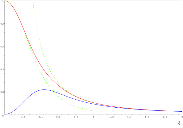
Figure 1: Mean survival probability $\left<P_{\nu_{1}\nu_{1}}\right>$ and fluctuations $\sigma(P)$ as functions of $\xi$. The dashed lines give the small $\xi$ ($\left<P_{\nu_{1}\nu_{1}}\right>\approx(U_{00})^{4})$, and the large $\xi$ ($\left<P_{\nu_{1}\nu_{1}}\right>\approx\frac{1}{\pi^{2}\xi^{2}}$) approximations.

The simplest toy model can now be compared to experimental data. For $\nu_{e}$, we are looking for a global 40 to 60% suppression at large $x$, as the simplest interpretation of the absence of $L/E$ dependence in the SuperKamiokande solar neutrinos data. This is possible because the Sun-Earth system is a very long-baseline system. As the solar core is large (typically, $x\sim 10^{5}$ and $\Delta x\sim 10^{2}>>1$ for solar neutrinos with $E\sim 1MeV$ and $R\sim 1mm$), fluctuations are completely washed away and the only observable effect will be an average suppression. Values of $\xi$ with $0.29<\xi<0.42$ fit the solar $\nu_{e}$ data.

However, we still should avoid MSW effects in the Sun or Earth. It turns out that this requirement and the Chooz constraint cannot be simultaneously respected.

The Chooz nuclear reactor experiment shows no $\overline{\nu}_{e}$ disappearance at a distance $L=1~{}km$ and a typical energy of 2 MeV. At fixed $\xi$, we can extract the largest allowed $x$ value for Chooz still fitting the data, or equivalently an upper limit for $1/R^{2}$. As $1/R$ controls the typical mass difference between two consecutive Kaluza-Klein levels, MSW resonant conversion will take place if $1/R$ is small compared to the MSW potential $V_{MSW}$. More precisely, this will happen if $1/R^{2}\leq 2EV_{MSW}$. Conversely, MSW effects can be avoided by putting a lower limit to $1/R^{2}$, which can then turn to be incompatible with the previous upper limit deduced from the Chooz constraint. The Fig. 2 shows that this is indeed the case in the toy model.

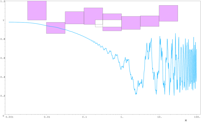
Figure 2: Comparison of the toy model with the $\nu_{e}$ constraints. The mean survival probability at large $x$ is fixed at 50% to fit the solar neutrinos. We have plotted the latest available experimental data we could find. The series of filled boxes show the $L/E$ dependence for the atmospheric $\nu_{e}$, as observed by SK (1$\sigma$). The data have been normalized by an overall 0.95 factor with respect to the raw data (instead of the usual $\sim$ 0.9 used by SK). The open box corresponds to the Chooz constraint. The error bar at $2\sigma$ level combines quadratically the statistical and systematic errors. The boxes cannot slide to the left without getting into the range of the MSW effect, showing thus a complete disagreement with the toy model.

One can also try to fit the $\nu_{\mu}$ data in the toy model (that is $\nu_{1}=\nu_{\mu}$). The Fig. 3 shows that a good agreement with the experimental data can be obtained for $\xi=0.4$.

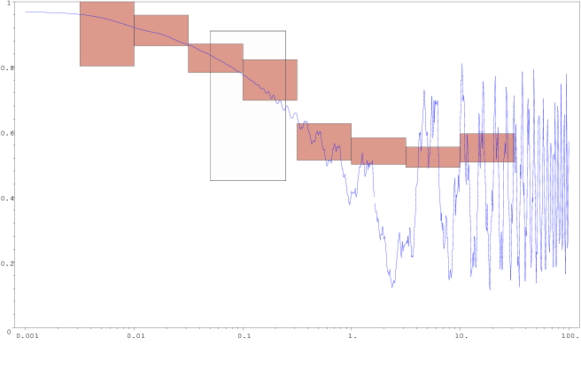
Figure 3: Comparison of the toy model with the $\nu_{\mu}$ constraints ($\xi=4/10$). The series of filled boxes show the $L/E$ dependence for the atmospheric $\nu_{\mu}$, as observed by Superkamiokande (1$\sigma$; the same 0.95 factor has been used). The open box corresponds to the K2K constraint. The error bar at $1\sigma$ level combines quadratically the statistical and systematic errors. The survival probability is in good agreement with the constraints, once an average on each energy ’bin’ is performed.

3 The 2-flavour model.

While almost as simple as the previous toy model, the 2-flavour model enables to accommodate most of the neutrino experimental data.

In addition to $\nu_{e}$, a second flavour neutrino, taken to be $\nu_{\mu}$, is included in the model. Only one linear combination of them, namely $\cos\theta\;\nu_{e}+\sin\theta\;\nu_{\mu}$ ($\theta$ is a new parameter : the mixing angle), which we call as previously $\nu_{1}$, is coupled to the bulk fermion. The Yukawa coupling proceeds exactly as in Eq. 1. The orthogonal linear combination, $\nu_{2}=-\sin\theta\;\nu_{e}+\cos\theta\;\nu_{\mu}$ remains massless and decouples.

The phenomenology of the 2-flavour model can be quite different from that of the toy model. Indeed, the mixing angle plays a crucial role in the survival probabilities of the flavour neutrinos.

$$P_{\nu_{e}\nu_{e}} = \cos^{4}\theta\;P_{\nu_{1}\nu_{1}}+\sin^{4}\theta+2\sin^{2}\theta\;\cos^{2}\theta\;\textrm{Re}\left(A_{\nu_{1}\nu_{1}}\right)$$

$$P_{\nu_{\mu}\nu_{\mu}} = \sin^{4}\theta\;P_{\nu_{1}\nu_{1}}+\cos^{4}\theta+2\sin^{2}\theta\;\cos^{2}\theta\;\textrm{Re}\left(A_{\nu_{1}\nu_{1}}\right)$$

Moreover, a transition $\nu_{e}\leftrightarrow\nu_{\mu}$ becomes possible and its probability is given by

$$P_{\nu_{e}\nu_{\mu}}=P_{\nu_{\mu}\nu_{e}}=\sin^{2}\theta\ \cos^{2}\theta\ (P_{\nu_{1}\nu_{1}}-2\textrm{Re}\left(A_{\nu_{1}\nu_{1}}\right)+1)$$

The 2-flavour model has 3 degrees of freedom, $(\xi,\theta,R)$, to fit the experimental data.

We first focus on the electronic neutrino data. As before, a global 40 to 60% suppression can account for the solar neutrino deficit. The contour plot of the mean $\nu_{e}$ survival probability in the plane $\xi-\theta$ is shown in Fig. 4, and defines a region of allowed values for the a-dimensional coupling $\xi$ and the mixing angle $\theta$.

Again, the Chooz constraint together with the no-MSW requirement forbids certain values for $(\xi,\theta)$, as can be seen in Fig. 4. A large allowed region of the parameter space still enables to fit all the $\nu_{e}$ experimental constraints. All solutions have a rather large mixing angle $\theta\sim\pi/4$. We can also verify that a mixing angle $\theta=0$ is indeed excluded.

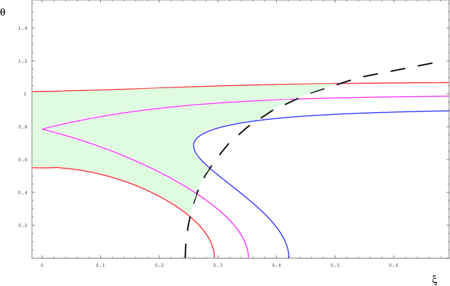
Figure 4: Region of values for $\xi$ and $\theta$ for which the solar and Chooz constraints for $\nu_{e}$ can be accommodated without MSW effect. The solid lines correspond (from top to bottom) to a solar neutrino mean survival probability of 60, 50, and 40%. The dashed line indicates the frontier of the MSW region in view of the Chooz constraint. The filled region gives the allowed $(\xi,\theta)$ values.

We can now discuss the constraints involving the muonic neutrinos. The $\nu_{\mu}$ disappearance experiment K2K, reveals some 30% deficit for 2 GeV neutrinos at a distance $L\simeq 250\ km$. As $x_{K2K}\simeq 1/4\cdot x_{Chooz}$, muonic neutrinos are expected to disappear more than electronic neutrinos. This requires $\theta>\pi/4$, and higher values of $\xi$ are preferred, as $P_{\nu_{e}\nu_{e}}-P_{\nu_{\mu}\nu_{\mu}}\propto(1-P_{\nu_{1}\nu_{1}})$. However, even for the maximal allowed $\xi$, the preliminary result of K2K can only be accommodated by taking the large statistical error into account. The Fig. 5 shows a possible fit for $\nu_{e}$ and $\nu_{\mu}$, which solves the solar neutrino problem, and simultaneously satisfies the Chooz and K2K constraints. It will be shown hereafter that this solution also fits the atmospheric neutrinos data.

To discuss the constraints coming from the atmospheric neutrinos, we recall that in the 2-flavour model, a transition $\nu_{e}\rightarrow\nu_{\mu}$ or $\nu_{\mu}\rightarrow\nu_{e}$ is possible. The transition probability, as shown in Fig. 5, becomes non negligible in the range of the atmospheric neutrinos. As the atmospheric neutrinos originate from the decay of the charged pions and kaons into muons and the subsequent decay of muons into electrons, the ratio of the neutrino initial fluxes $\frac{\phi^{(i)}_{\nu_{\mu}}}{\phi^{(i)}_{\nu_{e}}}$ is expected to be very close to 2, especially at low energy . Therefore, the expected atmospheric neutrino flux in the 2-flavour model is given by (we don’t distinguish between $\nu$ and $\overline{\nu}$)

$$\frac{\phi_{\nu_{e}}}{\phi^{(i)}_{\nu_{e}}}=P_{\nu_{e}\nu_{e}}+2\,P_{\nu_{\mu}\nu_{e}}$$ (7)

$$\frac{\phi_{\nu_{\mu}}}{\phi^{(i)}_{\nu_{\mu}}}=P_{\nu_{\mu}\nu_{\mu}}+1/2\,P_{\nu_{e}\nu_{\mu}}$$ (8)

As a result, the observed $\nu_{e}$ flux can be enhanced compared to the initial production flux. In Fig. 6, we see that this picture is in very good agreement with the SK results.

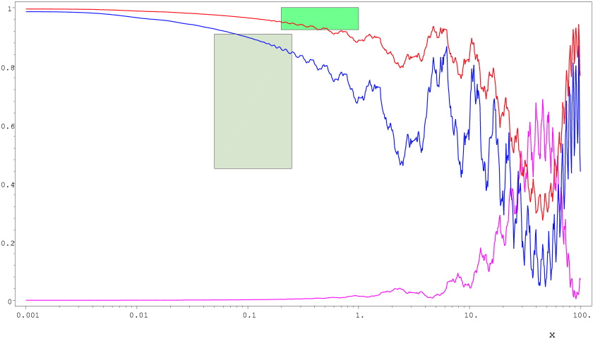
Figure 5: Comparison of the 2-flavour model with the Chooz and K2K constraints. (highest curve [red] is for $\nu_{e}$) $\xi=0.3$ and $\theta=1.05$, so that $\left<P_{\nu_{e}\nu_{e}}\right>\simeq 60\%$. The transition probability $P_{\nu_{e}\nu_{\mu}}$ is also depicted (lowest pink curve).

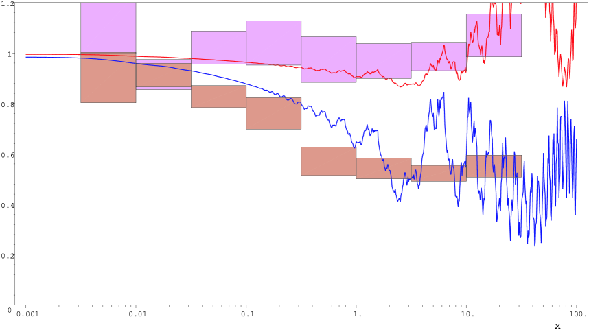
Figure 6: Expected atmospheric neutrino fluxes in the 2-flavour model and SK data. $\xi=0.3$ and $\theta=1.05$ as in Fig. 5. The initial flux $2\stackrel{{\scriptstyle(-)}}{{\nu_{\mu}}}+\stackrel{{\scriptstyle(-)}}{{\nu_{e}}}$ is normalized to 1 at $x=0$. The observed SK data has been normalized as in Fig. 2 The agreement with experimental data is quite remarkable.

We are left with the constraints of KARMEN and LSND. The negative result of the KARMEN experiment can easily be accommodated as $x_{KARMEN}\simeq 3\cdot 10^{-4}\ x_{Chooz}$. On the contrary, as $x_{LSND}\simeq 6\cdot 10^{-4}\ x_{Chooz}$, our model can never comply with the LSND results, for any allowed values of $\theta$ and $\xi$.

We have thus shown that all experimental data (with the exception of LSND) can be accommodated in the simple 2-flavour model.

The fit could however be invalidated in the near future, should the LSND signal be confirmed by an independent experiment. A critical test will also be provided by the improving accuracy of the K2K experiment. Finally, the 2-flavour model could also be invalidated if $\nu_{\tau}$ are explicitly detected. We also point out that the astrophysical bound could be evaded in this model, since the disappearance of $\nu_{e}$ or $\nu_{\mu}$ in the extra dimensions is never complete (see $\!{}^{{\bf?}}$).

4 Conclusions

We have shown that, in the context of theories with large extra dimensions, a flavour neutrino coupled to a bulk fermion can manifest surprising and interesting behaviours, combining both oscillation and disappearance. While a toy 1-flavour model is unable to fit all the experimental data, a simple 2-flavour model with only 3 free parameters meets most experimental constraints (except for LSND).

References

References

- [1] N. Cosme, J.-M. Frère, Y. Gouverneur, F.-S. Ling, D. Monderen and V. Van Elewyck, accepted in Phys. Rev. D, hep-ph/0010192.
- [2] N. Arkani-Hamed, S. Dimopoulos and G. Dvali, Phys. Lett. B 429 (1998) 263; I. Antoniadis, N. Arkani-Hamed, S. Dimopoulos and G. Dvali, Phys. Lett. B 436 (1998) 257.
- [3] N. Arkani-Hamed, S. Dimopoulos, G. Dvali and J. March-Russell, hep-ph/9811448; K. R. Dienes, E. Dudas, T. Gherghetta, Nucl. Phys. B 557 (1999) 25; R. N. Mohapatra, S. Nandi and A. Pérez-Lorenzana, Phys. Lett. B 466 (1999) 115; A. Das and O. C. Kong, Phys. Lett. B 470 (1999) 149; A. Lukas, P. Ramond, A. Romanino and G. G. Ross, hep-ph/0011295.
- [4] G. Dvali and A. Y. Smirnov, Nucl. Phys. B 563 (1999) 63.
- [5] R. N. Mohapatra and A. Pérez-Lorenzana, Nucl. Phys. B 593 (2001) 451; A. Lukas, P. Ramond, A. Romanino, G. G. Ross, Phys. Lett. B 495 (2000) 136; A. Ionnisian and J. W. Valle, hep-ph/9911349; E. Ma, G. Rajasekaran and U. Sarkar, Phys. Lett. B 495 (2000) 363.
- [6] A. Pérez-Lorenzana, hep-ph/0008333. Lectures given at the IX Mexican School on Particles and Fields, Metepec, Puebla, Mexico, August, 2000. To appear in the proceedings.
- [7] R. Barbieri, P. Creminelli and A. Strumia, Nucl. Phys. B 585 (2000) 28.
- [8] K. R. Dienes and I. Sarcevic, Phys. Lett. B 500 (2001) 133.