Hadron Production in Neutrino-Nucleon Interactions at High Energies

Abstract:

The multi-particle production at high energy neutrino- nucleon collisions are investigated through the analysis of the data of the experiment CERN-WA-025 at neutrino energy less than 260GeV and the experiments FNAL-616 and FNAL-701 at energy range 120-250 GeV. The general features of these experiments are used as base to build a hypothetical model that views the reaction by a Feynman diagram of two vertices. The first of which concerns the weak interaction between the neutrino and the quark constituents of the nucleon. At the second vertex, a strong color field is assumed to play the role of particle production, which depend on the momentum transferred from the first vertex. The wave function of the nucleon quarks are determined using the variation method and relevant boundary conditions are applied to calculate the deep inelastic cross sections of the virtual diagram.

1 Introduction

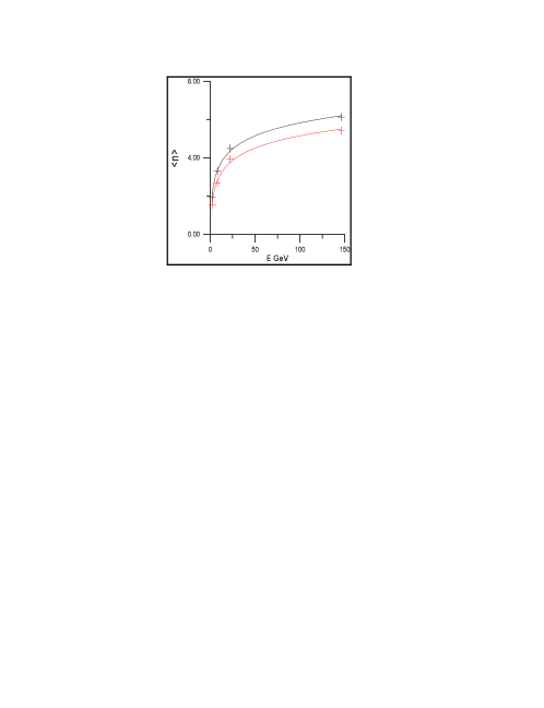
Figure 1: Average multiplicity of hadrons produced in $\nu-D$ (black +) and $\overline{\nu}-D$ (red +). The data concern the experiment CERN-WA-025. The solid lines are the parametric fitting curve of the form of $<n>=0.981*log(E)+1.318$ for $\nu-D$ experiment and $<n>=0.922*log(E)+0.909$ for the $\overline{\nu}-D$.

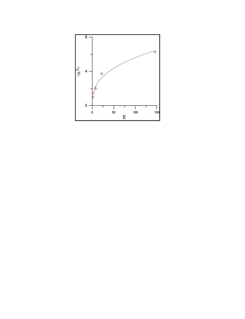
Figure 2: The second moment of the multiplicity of hadrons produced in $\nu-D$ (black +) and $\overline{\nu}-D$ (red +). The data concern the experiment CERN-WA-025. The solid line is the parametric fitting curve of the form $<n2>=1.075*E^{.358}$.

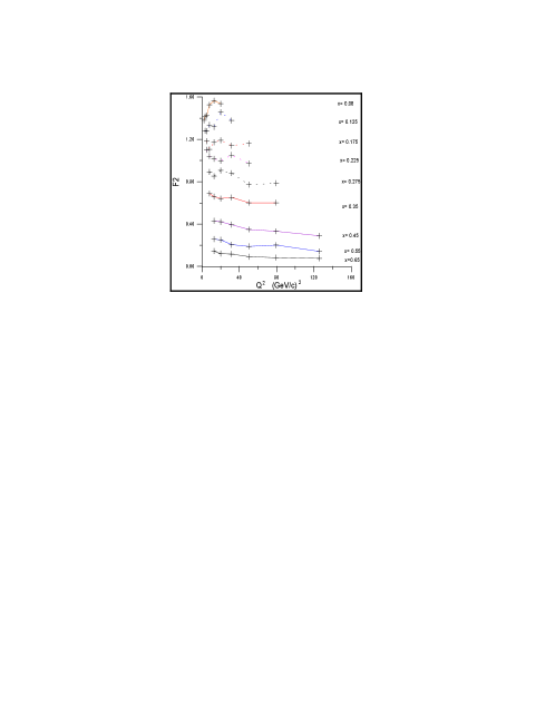
Figure 3: The structure function F2 of the ($\nu p$) collision of the experiments FNAL-616 and FNAL-701 at energy range 120-250 GeV, with Bjorken scaling variable $0.08<x<0.65$.

Observation of particles with large transverse momenta produced in high-energy collisions of hadrons and nuclei provides information about the properties of quark and gluon interactions. As follows from numerous studies in relativistic physics [1, 2, 3], a common feature of the processes is the local character of the hadron interactions. This leads to a conclusion about dimensionless constituents participating in the collisions. On the other hand, the deep inelastic interactions of leptons with nuclei may reveal facts that relate the nature of particle production at lepton processes to that produced by hadrons. All these reasons had persuaded us to pursue the recent experiments of the neutrinos and antineutrinos with nucleons and nuclei to extract the general features of such collisions that enable to set up a relevant phenomenological model. The CERN experiment CERN-WA-025 [4], and the Fermi National lab experiments FNAL-616 [5] and FNAL-701 [6] are good samples to consider for examination. The first conclusion extracted from these experiments is the logarithmic relation between the average charged particle multiplicity and the lab energy of the incident neutrino as demonstrated by Fig. (1). The figure shows also that neutrinos ($\nu$) produce more particles than antineutrinos ($\overline{\nu}$) at the same incident energy and in both cases the yield of particles is much less than the corresponding case of hadron nucleon collisions [7]. Moreover, Fig. (2) shows that the values of the 2nd moment does not depend on the type of the projectile whether it is $\nu$ or $\overline{\nu}$ and this moment has the exponential form similar to that of hadron nucleon. Finally, Figures (3 , 4) show that F2 and x F3 are approximately independent on the momentum transfer square Q2, but instead depend on the Bjorken scalar variable x. In this work, a hypothetical model is proposed assuming a Feynman diagram of two vertices. At the first of which, the incident neutrino interacts with one of the nucleon constituent quarks by weak interaction and exchanges a heavy boson W or Z. The first vertex is considered as the source, which supply the second vertex with energy that is used to create pairs of hadrons through strong interaction. Of course, the charged and neutral currents due to W and Z in this case have their own property that is responsible to different result of the hadrons. The paper is organized as follows: In section 2, we present the scenario of the model as well as the results and discussion. Brief summary and conclusive remarks are given in section 3.

2 The Proposed Model

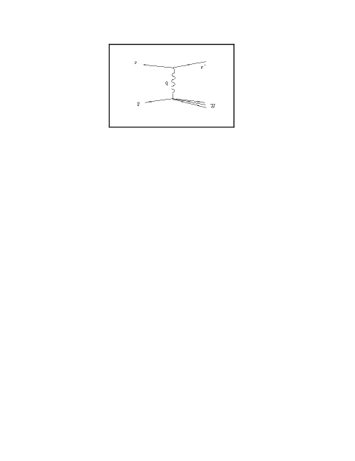
Figure 5: Feynman diagram describes the multiparticle production in $\nu-N$ collisions.

The problem of multi particle production in $\nu$-N collision is classified into two main parts. The first is to propose a relevant diagram to describe the process and specify the matrix element at its vertices. The second is to specify the wave function of the constituent particles of the target. Our strategy is to use a Feynman diagram as shown in Fig. (5) with two vertices. At the first, a weak interaction takes place and a strong interaction holds the second vertex. On the other hand, we follow the quantum variation method [8] to determine the parton wave function. Consider a two-dimensional Minkowski space, and we define the null momentum [9] $p$ as $p=p_{0}-p_{l}$ where $p_{o}$ represents the total energy and $p_{l}$ is the longitudinal momentum, so that the mass shell condition for a particle of mass m: $p_{0}^{2}=p_{l}^{2}+m^{2}$ is replaced by $p_{0}=\frac{1}{2}(p+\frac{m^{2}}{p})$ . In QCD, the force between quarks is due to the exchange of gluons, which are massless bosons, and corresponds to the photons in QED. The long-range field between quarks may be considered as linear field in null coordinates and has a propagator $1/q^{2}$ in momentum space. Let us consider the nucleon as a relativistic quantum system of multiparticles. So that the nucleon is described in terms of wave function that depends on quantum numbers concerning the quarks (momentum, spin, color, flavor). The values of these parameters are determined to minimize the total energy of the quark system of the nucleon. Since the quarks forming the nucleon have spin=1/2 and the nucleon is colorless, so it is convenient to write the parton wave function as $\widetilde{\Psi}(a,\alpha,p)$ , where $a$ is the flavor (up or down), $\alpha$ is the color quantum number and $p$ is the momentum in the null space. Then the nucleon wave function for $N$ partons is $\widetilde{\Psi}(a_{1},\alpha_{1},p_{1};...;a_{N},\alpha_{N},p_{N})$ and should be anti-symmetric under interchange of a pair of quarks, as the nucleons are Fermions. However, since the baryon is invariant under color, the wave function must be completely in color alone

$$\widetilde{\Psi}(a_{1},\alpha_{1},p_{1};...;a_{N},\alpha_{N},p_{N})=\frac{\varepsilon_{\alpha_{1}...\alpha_{N}}}{\sqrt{N!}}\widetilde{\Psi}(a_{1},p_{1};...;a_{N},p_{N})$$ (1)

The corresponding nucleon wave function in the position space is $\Psi(\{{a_{i},r_{i}\}})$ which is the Fourier transform of $\widetilde{\Psi}(a_{1},p_{1};...;a_{N},p_{N})$ . If $\mu_{a}$ is the quark mass and the linear potential between a quark pair is $V(r_{i}-r_{j})=\frac{g^{2}}{2}(r_{i}-r_{j})$, where $g^{2}$ is the coupling constant, then the total energy of the nucleon is

$$\zeta_{N} = \sum_{a_{1}..a_{N}}\int_{0}^{\infty}\sum_{i=1}^{N}(p_{i}+\frac{\mu_{i}^{2}}{p_{i}})|\widetilde{\Psi}(a_{1}..a_{N};..p_{1}..p_{N})|^{2}\frac{dp_{1}..dp_{N}}{(2\pi)^{N}}+$$ (2)

$$+\frac{g^{2}}{2}\sum_{a_{1}..a_{N}}\int_{-\infty}^{\infty}\sum_{i\neq j}^{N}(r_{i}-r_{j})|\Psi(a_{1}..a_{N};..r_{1}..r_{N})|^{2}dr_{1}...dr_{N}$$

Starting with the simplest parametric form of the quark wave function,

$$\widetilde{\Psi}(p)=C\exp(-ap)$$ (3)

where $a>0$ and $p>=0$ and the Fourier transform is

$$\Psi(r)=\frac{C^{\prime}}{(r+ia)^{2}}$$ (4)

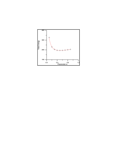
Figure 6: The variation of the total energy of the assembly of the quarks forming the nucleon shows that it has a minimum at a parameter value $a=0.5$

Where $C$and $C^{\prime}$are normalization constants, while $a$ is a fitting parameter. It is found that $a=0.5$ gives minimum value of the total energy as shown in Fig.(6).

A more reasonable quark wave function with two variation parameters $\alpha$and $\beta$, is

$$\widetilde{\Psi}(p)=Cp^{\alpha}(1-p)^{\beta}$$ (5)

Again, inserting Eq. (2.4) in Eq. (2.1), this results that the total energy $E_{tot}$of the quark assembly of the nucleon shows multiple minima corresponding to different energy levels whose eigen parameters $\alpha$and $\beta$are listed in Table (1). The range of the null momentum $p$extends from zero up to $P_{max}$. It is more convenient to express the wave function and all other physical quantities in terms of the scaling Bjorken variable $x=p/P_{\max}$where $0<x<1$.

Table (1)

Parton state	$\alpha$	$\beta$	Energy (arbitrary unit)
E0	3.6	3.6	3.45x10-6
E1	2.9	3.7	6.76x10-6
E2	2.7	3.7	9.54x10-6
E3	2.2	3.4	4.60x10-6
E4	2.1	3.1	4.70x10-6

The ground state E0 has equal values in the parameters $\alpha$and $\beta$which means that the state has line symmetry about $x=0.5$, in other words, the probability that a parton has a value $x$is equal to that of $(1-x)$. The symmetry breaks at the higher-up states, where the probability increases towards the deep inelastic $x<0.5$. The wave functions defined by Eqs. (2.2) and (2.4) are to be used to calculate the scattering amplitude $\Gamma$due to the diagram Fig. (5) as,

$$\Gamma_{tot}=\prod_{i}\Gamma_{i}$$ (6)

where $\Gamma_{i}$is the scattering amplitude at the i^thvertex of the diagram. Since the diagram contains only two vertices, where a weak interaction holds the first and a strong one at the second, and each one is associated with its relevant propagator, so that $\Gamma_{tot}$may be written as,

$$\Gamma_{tot}(x,q^{2})=\frac{1}{q^{2}+M_{W,Z}^{2}}\exp(-\gamma q^{2})|\widetilde{\Psi}(x)|^{2}$$ (7)

Eq. (2.6) includes three factors, the first is the propagator of the weak field in which $M_{W,Z}$represents the mass of the exchange Boson [10] for the charged $W^{\pm}$or the neutral $Z^{0}$current. The second factor is the propagator for the strong field or sometimes known as the profile function [11]. The third factor is the probability density. The problem of particle production is to be viewed through the relativistic phase space. Following the scheme of Ref. [12], it is easy to define the cross section of finding n-particles in the final state with total center of mass energy $W$, $W^{2}=(p_{a}+p_{b})^{2}$

$$\sigma_{n}=\frac{1}{F}\int...\int\prod_{i}\{\frac{d^{3}p_{i}}{2E_{i}}\}\delta^{4}(p_{a}+p_{b}-\sum p_{i})|\Gamma(p_{i})|^{2}$$ (8)

Where $F$represents the incident flux and the delta function is to conserve the four-vector momentum at the $2^{nd}$vertex of the reaction. It also restricts the integration over a surface of 3n-4dimensional space. The multi-dimensional integration in Eq. (2.7) may be solved using the Monte Carlo technique. However the volume of such a sphere may be approximated at extremely high energy as,

$$\sigma_{n}=\frac{1}{F}\frac{(\pi/2)^{n-1}}{(n-1)!(n-2)!}W^{n-2}|\Gamma(p)|^{2}$$ (9)

Transforming Eq. (2.7) from the momentum space to the Bjorken scaling $x$and writing the energy $W$in terms of the kinematical variables of diagram (5), $W^{2}=m^{2}+q^{2}(\frac{1}{x}-1)$, then

$$\sigma_{n}(x,q^{2})=\frac{1}{F}\frac{(\pi/2)^{n-1}}{(n-1)!(n-2)!}[m^{2}+q^{2}(\frac{1}{x}-1)]^{n-2}|\Gamma(x,q^{2})|^{2}$$ (10)

The implementation of Eq. (2.9) results in Fig. (7), which shows that the cross section of production of n-particles depends appreciably on $x$and weakly on $q^{2}$. The decrease of $x$means going towards the deep inelastic, which offer more fraction of energy for creation of particles and this increases the peak of the multiplicity towards higher values. The overall multiplicity distribution is found by integrating over x from 0 to 1 and over $q^{2}$from . A cutoff value of $q^{2}$is necessary to keep the system in the physical region of the phase space. The cutoff ratio is taken as a free parameter in this model to fit the experimental data. The multiplicity distributions of secondary hadrons are demonstrated in Fig. (8) for ?-energies of 2, 8, 22 and 146 GeV, the average values of each are listed in Table (2) with the considered parameters. The comparison with the experimental data shows very good agreement. The cross section $\sigma_{n}(x,q^{2})$is recalculated again using the parton wave function as in Eq. (2.4) for the first 3- parton states only E0, E1 and E2 with the corresponding parameters as in Table (1). The results are given in Table (3) for the average multiplicity compared with the experimental values that show also good agreement. In fact the comparison with the average value of the multiplicity is not enough to reflect the validity of a hypothetical model, nevertheless, it may indicate that the work is going in the right way. In the forth- coming paper we managed to take into account the effect of the exchange whether it is the neutral boson $Z^{0}$or the charged $W^{\pm}$. This may be used to interpret the increase of the yield in $\nu$-N collisions than the case of $\overline{\nu}$-N. Also the calculation of the differential cross section $d^{2}\sigma/dxdq^{2}$may give more information on such reactions.

Table (2)

Cutoff	Eν	a	¡n¿exp	¡n¿th
0.075	2	.5	1.97	2.1
0.070	8	.5	3.30	3.31
0.020	22	.5	4.50	4.35
0.001	146	.5	6.14	6.17

Table (3)

¡n¿exp	$\gamma$(E0)	$\gamma$(E1)	$\gamma$(E2)	¡n¿th
1.97	1	1.1	1.15	2.10
3.30	0.31	0.36	0.37	3.31
4.50	0.20	0.26	0.27	4.35
6.14	0.03	0.033	0.033	6.17

3 Concluding Remarks.

• The average multiplicity of hadrons produced in $\nu$-nucleon interactions has a logarithmic dependence on the energy of the incident neutrino. The yield in $\nu$-N is slightly greater than the corresponding figure in $\overline{\nu}$-N.

• The $\nu$-N interaction may successfully described by a Feynman diagram of two vertices. A weak interaction holds the first and a strong interaction at the second where hadrons are created. W and Z bosons are assumed as the exchange particles in the weak interaction.

• The first vertex of the Feynman diagram is assumed as the source, which supply the energy to the second vertex. That energy is responsible for hadron creation. The rate of energy transfer is controlled by the matrix element of weak interaction at the first vertex.

• The average multiplicity of produced hadrons is strongly dependent on the Bjorken scaling variable $x$ and weakly on the momentum transfer $q^{2}$.

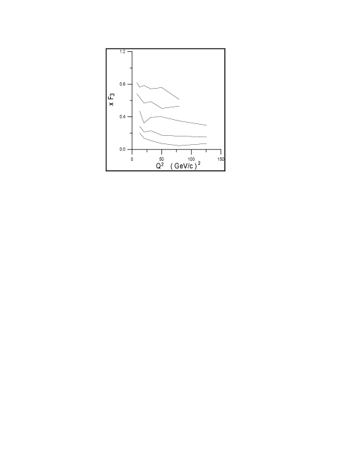
Figure 4: The structure function xF3 of the ($\nu p$) collision of the experiments FNAL-616 and FNAL-701 at energy range 120-250 GeV, with Bjorken scaling variable $0.08<x<0.65$.

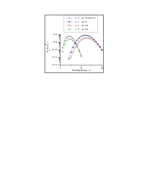
Figure 7: The multiplicity distribution of charged secondaries in $\nu p$ collision as a function of both x and $q^{2}$.

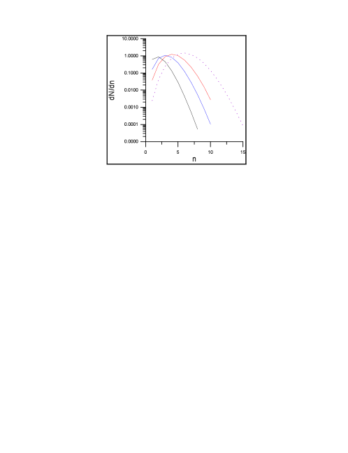
Figure 8: The overall multiplicity distribution of charged secondaries produced in $\nu p$ collision as predicted by the model.

References

- [1] Proceedings of the X International Conference on Ultra-Relativistic Nucleus-Nucleus Collisions, Borlange, Sweden, 1993 [Nucl. Phys. A566, 1c (1994)].
- [2] Proceedings of the XII International Conference on Ultra-Relativistic Nucleus-Nucleus Collisions, Heidelberg, Germany, 1996 [Nucl. Phys. A610, 1c (1996)].
- [3] Proceedings of the XIV International Conference on Ultra-Relativistic Nucleus-Nucleus Collisions, Torino, Italy, 1999 [Nucl. Phys. A661, 1c (1999)].
- [4] A.G. Tenner et.al.; IL Nuovo Cimento, 105A (1992) 1001; Phys. Rev. C49 (1994) 2379
- [5] Oltman, Z.Phys. C53,(1992),51; I.M. Blair, Phys. Rev. Lett 51(1983)343 Oltman, Z.Phys. C53,(1992),51; I.M. Blair, Phys. Rev. Lett 51(1983)343
- [6] A.E. Aasratyan, Z.Phys. C58 (1993) 55
- [7] M.T. Hussein et.al., Canad. J. Phys.
- [8] S.G.Rajeev, Lecture in Summer School in High Energy and cosmology Vol II, ICTP, Trieste, Italy (1991).
- [9] O.T. Turgut and S.G.Rajeev, Comm.Math.Phys. 192(1998) 493
- [10] P. Abreu et. Al., (DELPHI Collaboration), Eur Phys J C18 (2000) 203; Phys. Lett B499(2001)23
- [11] M.K. Hegab, M.T. Hussein and N.M. Hassan, Z.Physics A 336,(1990) 345
- [12] M.T. Hussein, IL Nuovo Cimento 106 A (1993) 481