Thermal Gauge Field Theories

Thermal Gauge Field Theories

Abstract: The real- and imaginary-time-formalisms of thermal field theory and their extension to gauge theories is reviewed. Questions of gauge (in-)dependence are discussed in detail, in particular the possible gauge dependences of the singularities of dressed propagators from which the quasiparticle spectrum is obtained. The existing results on next-to-leading order corrections to non-Abelian screening and dispersion laws of hard-thermal-loop quasiparticles are surveyed. Finally, the role of the asymptotic thermal masses in self-consistent approximations to thermodynamic potentials is described and it is shown how the problem of the apparently poor convergence of thermal perturbation theory might be overcome.

1 Overview

The theoretical framework for describing ultrarelativistically hot and dense matter is quantum field theory at finite temperature and density. At sufficiently high temperatures and densities, asymptotic freedom should make it possible to describe even the fundamental theory of strong interactions, quantum chromodynamics (QCD), through analytical and mostly perturbative means. These lectures try to cover both principal issues related to gauge freedom as well as specific problems of thermal perturbation theory in non-Abelian gauge theories.

After a brief review of the imaginary- and real-time formalisms of thermal field theory, the latter is extended to gauge theories. Aspects of different treatments of Faddeev-Popov ghosts and different gauge choices are discussed for general non-Abelian gauge theories, both in the context of path integrals and in covariant operator quantization. The dependence of the formalism on the gauge-fixing parameters introduced in perturbation theory is investigated in detail. Only the partition function and expectation values of gauge-invariant observables are entirely gauge independent. Beyond those it is shown that the location of singularities of gauge and matter propagators, which define screening behaviour and dispersion laws of the corresponding quasi-particle excitations, are gauge independent when calculated systematically.

At soft momentum scales it turns out to be necessary to reorganize perturbation theory such that (at least) the contribution of the so-called hard thermal (dense) loops (HTL/HDL) is resummed. The latter form a gauge-invariant effective action, and their gauge-fixing independence is verified. The existing results of such resummations on the modification of the spectrum of HTL quasi-particles at next-to-leading order (NLO) are reviewed, and a few cases discussed in more detail, with special attention given to gauge dependence questions.

It is shown how screening and damping phenomena become logarithmically sensitive to the strictly nonperturbative physics of the chromomagnetostatic sector, with the exception of the case of zero 3-momentum. In particular the definition of a non-Abelian Debye mass is discussed at length, also with respect to recent lattice results.

Real parts of the dispersion laws of quasiparticle excitations, on the other hand, are infrared-safe at NLO. However, as the additional collective modes of longitudinal plasmons and fermionic “plasminos” approach the light-cone, collinear singularities arise, signalling a qualitative change of the dispersion laws and requiring additional resummations. At high momenta only the regular modes of the fermions and the spatially transverse ones of the gauge bosons remain and they tend to asymptotic mass hyperboloids. The NLO corrections to the asymptotic thermal masses play an interesting role in a self-consistent reformulation of thermodynamics in terms of weakly interacting quasi-particles. In this application, the problem of poor convergence of resummed thermal perturbation theory resurfaces, but it is shown that it may be overcome through approximately self-consistent gap equations.

2 Basic Formulae

Before coming to quantum field theories and gauge theories in particular, let us begin by recalling some relevant formulae from quantum statistical mechanics.

We shall always consider the grand canonical ensemble, in which a system in equilibrium can exchange energy as well as particles with a reservoir such that only mean values of energy and other conserved quantities (baryon/lepton number, charge, etc.) are prescribed through Lagrange multipliers $\beta=1/T$ and $\alpha_{i}=-\beta\mu_{i}$, respectively, where $T$ is temperature and $\mu_{i}$ are the various chemical potentials associated with a set of commuting conserved observables $\hat{N}_{i}=\hat{N}_{i}^{\dagger}$ satisfying $[\hat{N}_{i},\hat{N}_{j}]=0$ and $[\hat{H},\hat{N}_{i}]=0$, where $\hat{H}$ is the Hamiltonian.

The statistical density matrix is given by

$$\hat{\varrho}={Z^{-1}}\exp\left[-\alpha_{i}\hat{N}_{i}-\beta\hat{H}\right]\equiv{Z^{-1}}\exp\Bigl{[}-\beta(\underbrace{\hat{H}-\mu_{i}\hat{N}_{i}}_{\mbox{$=:\bar{H}$}})\Bigr{]}$$ (1)

where $Z$ is the partition function

$$Z=Z(V,T,\mu_{i})={\rm Tr}\;\mathrm{e}^{-\beta\bar{H}}.$$ (2)

and the thermal expectation value (ensemble average) of an operator $\hat{A}$ is given by

$$\langle\hat{A}\rangle={\rm Tr}[\hat{\varrho}\hat{A}]\,.$$ (3)

When total energy and particle numbers are extensive quantities, i.e. proportional to the volume $V$, one also has $\ln Z\propto V$, and since we shall be interested in the limit $V\to\infty$, it is preferable to define intensive quantities. The most important one is the thermodynamic pressure

$$P=\frac{1}{\beta V}\ln Z$$ (4)

which up to a sign is identical to the free energy density $F/V=-P$ ($F$ is also referred to as the thermodynamic potential $\Omega$).

Other thermodynamic (or should one say thermo-static?) quantities can be derived from $P$, such as particle/charge densities

$$n_{i}=\frac{1}{V}\langle\hat{N}_{i}\rangle={\partial P\over\partial\mu_{i}},$$ (5)

energy density

$$\varepsilon=E/V=\frac{1}{V}\langle\hat{H}\rangle=-\frac{1}{V}{\partial\ln Z\over\partial\beta}=-{\partial(\beta P)\over\partial\beta}$$ (6)

(at fixed $\alpha_{i}$), and entropy density (which will play a prominent role at the very end of these lectures)

$$s = S/V={1\over V}\langle-\ln\hat{\varrho}\rangle={1\over V}\ln Z+{\beta\over V}\langle\hat{H}-\mu_{i}\hat{N}_{i}\rangle$$ (7)

$$= {\partial P\over\partial T}=\beta(P+\varepsilon-\mu_{i}n_{i})$$ (8)

In the latter equations one recognizes the familiar Gibbs-Duhem relation

$$E=-PV+TS+\mu_{i}N_{i},$$ (9)

which explains why $P$ was defined as the (thermodynamic) pressure. A priori, the hydrodynamic pressure, which is defined through the spatial components of the energy-momentum tensor through ${1\over 3}\langle T^{ii}\rangle$, is a separate object. In equilibrium, it can be identified with the thermodynamic one through scaling arguments Landsman:1987uw , which however do not allow for the possibility of scale (or “trace”) anomalies that occur in all quantum field theories with non-zero $\beta$-function (such as QCD). In Drummond:1999si it has been shown recently that the very presence of the trace anomaly can be used to prove the equivalence of the two in equilibrium.

All the above relations continue to hold in (special) relativistic situations, namely within the particular inertial frame in which the heat bath is at rest. In other inertial frames one has the additional quantity of heat-bath 4-velocity $u^{\mu}$, and one can generalize the above formulae by replacing $V=\int\!d^{3}x\to\int\limits_{\Sigma\perp u}\!d\Sigma_{\mu}u^{\mu}$, and the operators in (1) by

$$H\to\int\!d\Sigma_{\mu}T^{\mu\nu}u_{\nu},\qquad N_{i}\to\int\!d\Sigma_{\mu}j^{\mu}_{i}.$$ (10)

$\alpha_{i}$ and $\beta$ are Lorentz scalars (i.e., temperature is by definition measured in the rest frame of the heat bath). The partition function can then be written in covariant fashion as Israel:1981

$$Z={\rm Tr}\left[\exp\int\!d\Sigma_{\mu}\left(-\hat{T}^{\mu\nu}\beta_{\nu}-\hat{j}^{\mu}_{i}\alpha_{i}\right)\right],$$ (11)

where we have introduced an inverse-temperature 4-vector $\beta^{\mu}\equiv\beta u^{\mu}$.

However, in what follows we shall most of the time remain in the rest frame of the heat bath where $u^{\mu}=\delta^{\mu}_{0}$.

3 Complex Time Paths

With a complete set of states given by the eigenstates of an operator $\hat{\varphi}$, $\hat{\varphi}|\varphi\rangle=\varphi|\varphi\rangle$, we formally write

$$Z={\rm Tr}\left[\mathrm{e}^{-\beta\hat{H}}\right]=\sum_{\varphi}\langle\varphi|\mathrm{e}^{-\beta\hat{H}}|\varphi\rangle.$$ (12)

In field theory, we shall boldly use the field operator $\hat{\varphi}=\hat{\varphi}(t,\vec{x})$ in the Heisenberg picture and write $|\varphi\rangle$ for its eigenstates at a particular time.

Using that the transition amplitude $\langle\varphi_{1}|\mathrm{e}^{-{\rm i}\hat{H}(t_{1}-t_{0})}|\varphi_{0}\rangle$ [the overlap of states that have eigenvalue $\varphi_{0}(\vec{x})$ at time $t_{0}$ with states that have eigenvalue $\varphi_{1}(\vec{x})$ at time $t_{1}$] has the path integral representation

$$\langle\varphi_{1}|\mathrm{e}^{-{\rm i}\hat{H}(t_{1}-t_{0})}|\varphi_{0}\rangle$$ (13)

$$\quad={\cal N}\!\!\!\!\!\!\!\!\int\limits_{\varphi(t_{0},\vec{x})=\varphi_{0}\atop\varphi(t_{1},\vec{x})=\varphi_{1}}\!\!\!\!\!\!\!\!{\cal D}\varphi\;\exp{\rm i}\int_{t_{0}}^{t_{1}}\!\!dt\int\!d^{3}x\,{\cal L}(\varphi,\partial\varphi)$$ (14)

we can give a path integral representation for $Z$ that takes care of the density operator by setting $t_{1}=t_{0}-{\rm i}\beta$, and of the trace by integrating over all configurations with $\varphi_{1}=\varphi_{0}$.

When there is a chemical potential $\mu\not=0$, we have $\hat{H}\to\bar{H}=\hat{H}-\mu\hat{N}$ and this implies $L\to L+\mu N$ if there are no time derivatives in $N$, and we have

$$Z={\cal N}\int{\cal D}\varphi\;\exp{\rm i}{\int_{t_{0}}^{t_{0}-{\rm i}\beta}\!\!\!\!dt}\int\!d^{3}x\,\bar{\cal L}$$ (15)

where the path integral is over all configurations periodic in imaginary time, $\varphi({t_{0}},\vec{x})=\varphi({t_{0}-{\rm i}\beta},\vec{x})$.

In this formula, real time has apparently been fixed to $t_{0}$ and replaced by an imaginary time flow which is periodic with period $\beta$, the inverse temperature. In equilibrium thermodynamics, this seems only fitting as nothing depends on time in strict equilibrium.

However, we have not really required time to have a fixed real part. We have made the end point complex with the same real part, but the integration over $t$ in (15) need not be a straight line with fixed $t_{0}$. Instead we shall consider a general complex time path, and this allows us to define Green functions by the path integral formula

$$\langle\mathrm{T}_{c}\hat{\varphi}_{1}\cdots\hat{\varphi}_{n}\rangle={\cal N}\int{\cal D}\varphi\,\varphi_{1}\cdots\varphi_{n}\exp{{\rm i}\int\limits_{\cal C}\!dt\!\int\!d^{3}x\,\bar{\cal L}}$$ (16)

where $\mathrm{T}_{c}$ now means contour ordering along the complex time path ${\cal C}$ from $t_{0}$ to $t_{0}-{\rm i}\beta$ such that $t_{i}\in{\cal C}$, and $t_{1}\succeq t_{2}\succeq\cdots\succeq t_{n}$ with respect to a monotonically increasing contour parameter.

Through quantities like (16) we are not restricted to time-independent, thermo-static questions, but may also consider small perturbations of the equilibrium (response theory).

The time path introduced in (16) is in fact not completely arbitrary. Considering spectral representations in the energy representation leads to the conclusion Landsman:1987uw that $\cal C$ has to be such that the imaginary part of $t$ is monotonically decreasing. This is a necessary condition for analyticity; in the limiting case of a constant imaginary part along (parts of) the contour, distributional quantities (generalized functions) arise.

Except for the periodic boundary conditions with regard to the end points of $\cal C$ (which become anti-periodic for fermionic field operators and Grassmann-valued “classical” fields), the path integral formula (16) is formally identical to the familiar one from $T=0$ and $\mu=0$.

Indeed, perturbation theory is set up in the usual fashion. Using the interaction-picture representation one can derive

$$\langle\mathrm{T}_{c}\mathcal{O}_{1}\cdots\mathcal{O}_{n}\rangle={Z_{0}\over Z}\langle\mathrm{T}_{c}\mathcal{O}_{1}\cdots\mathcal{O}_{n}\,\mathrm{e}^{{\rm i}\!\int_{\mathcal{C}}\mathcal{L}_{I}}\rangle_{0},$$ (17)

where $\mathcal{L}_{I}$ is the interaction part of $\cal L$, and the correlators on the right-hand-side can be evaluated by a Wick(-Bloch-DeDominicis) theorem:

$$\langle\mathrm{T}_{c}\mathrm{e}^{{\rm i}\!\int_{\mathcal{C}}d^{4}x\,j\varphi}\rangle_{0}=\exp\{-{1\over 2}\int_{\mathcal{C}}\int_{\mathcal{C}}d^{4}x\,d^{4}x^{\prime}j(x)D^{c}(x-x^{\prime})j(x^{\prime})\},$$ (18)

where $D^{c}$ is the 2-point function and this is the only building block of Feynman graphs with an explicit $T$ and $\mu$ dependence. It satisfies the KMS (Kubo-Martin-Schwinger) condition

$$D^{c}(t-{\rm i}{\beta})=\pm\mathrm{e}^{-{\mu}{\beta}}D^{c}(t),$$ (19)

stating that $\mathrm{e}^{{\rm i}\mu t}D(t)$ is periodic (antiperiodic) for bosons (fermions).

3.1 Imaginary-Time (Matsubara) Formalism

The simplest possibility for choosing the complex time path is the straight line from $t_{0}$ to $t_{0}-{\rm i}\beta$, which is named after Matsubara Matsubara:1955ws who first formulated perturbation theory based on this contour. It is also referred to as imaginary-time formalism (ITF), because for $t_{0}=0$ one is exclusively dealing with imaginary times.

Because of the (quasi-)periodicity (19), the propagator is given by a Fourier series

$$D^{c}(t)={1\over-{\rm i}{\beta}}\sum_{\nu}\tilde{D}(z_{\nu})\mathrm{e}^{-{\rm i}z_{\nu}t},\quad\tilde{D}(z_{\nu})=\int_{0}^{-{\rm i}{\beta}}\!\!\!dt\,D^{c}(t)\mathrm{e}^{{\rm i}z_{\nu}t}$$ (20)

with discrete complex (Matsubara) frequencies

$$z_{\nu}=2\pi{\rm i}\nu/{\beta}+{\mu},\quad\nu\in\left\{\begin{array}[]{ll}\mathbb{Z}&\mbox{bos.}\\ \mathbb{Z}-{1\over 2}&\mbox{ferm.}\\ \end{array}\right.$$ (21)

The transition to Fourier space turns the integrands of Feynman diagrams from convolutions to products as usually, with the difference that there is no longer an integral but a discrete sum over the frequencies, and compared to standard momentum-space Feynman rules one has

$$\int{d^{4}k\over{\rm i}(2\pi)^{4}}\to\beta^{-1}\sum_{\nu}\int{d^{3}k\over i(2\pi)^{3}},\qquad{\rm i}(2\pi)^{4}\delta^{4}(k)\to\beta(2\pi)^{3}\delta_{\nu,0}\delta^{3}(k).$$ (22)

However, all Green functions that one can calculate in this formalism are initially defined only for times on $\cal C$, so all time arguments have the same real part. The analytic continuation to different times on the real axis is, however, frequently a highly non-trivial task Landsman:1987uw , so that it can be advantageous to use a formalism that supports real time arguments from the start.

3.2 Real-Time (Schwinger-Keldysh) Formalism

In the so-called real-time formalisms, the complex time path $\cal C$ is chosen such as to include the real-time axis from an initial time $t_{0}$ to a final time $t_{f}$. Since we have to end up at $t_{0}-{\rm i}\beta$, this requires a further part of the contour to run backward in real time Schwinger:1961qe ; Bakshi:1963 and to finally pick up the imaginary time $-{\rm i}\beta$. There are a couple of paths $\cal C$ that have been proposed in the literature. The oldest one due to Keldysh Keldysh:1964ud is shown in Fig. 1, and this is also (again) the most popular one.

Figure 1: Complex time path in the Schwinger-Keldysh real-time formalism

Clearly, if none of the field operators in (16) has time argument on $\mathcal{C}_{1}$ or $\mathcal{C}_{2}$, the contributions from these parts of the contour simply cancel and one is back to the ITF.

On the other hand, if $t_{0}\to-\infty$, and all operators have finite real time arguments, the contribution from contour $\mathcal{C}_{3}$ decouples because from the spectral representation one has for instance for the propagator connecting contour $\mathcal{C}_{1}$ and $\mathcal{C}_{3}$

$$D^{13}(k,t-(t_{0}-{\rm i}\lambda))=\int\limits_{-\infty}^{\infty}d\omega\,\mathrm{e}^{-{\rm i}\omega(t-t_{0})}{\sigma\mathrm{e}^{\lambda\omega}\over\mathrm{e}^{\beta\bar{\omega}}-1}\varrho(k,\omega)\stackrel{{\scriptstyle t_{0}\to-\infty}}{{\longrightarrow}}0$$ (23)

for $\lambda\in(0,\beta)$ by Riemann-Lebesgue Landsman:1987uw .

With only $\mathcal{C}_{1}$ and $\mathcal{C}_{2}$ contributing, the action in the path integral decomposes according to

$$\int\limits_{\mathcal{C}_{1}\cup\,\mathcal{C}_{2}}\mathcal{L}(\varphi)=\int_{-\infty}^{\infty}dt\,\mathcal{L}(\varphi^{(1)})-\int_{-\infty}^{\infty}dt\,\mathcal{L}(\varphi^{(2)})$$ (24)

where we have to distinguish between fields of type 1 (those from contour $\mathcal{C}_{1}$) and of type 2 (those from contour $\mathcal{C}_{2}$) because of the prescription of contour ordering in (16). From (24) it follows that type-1 fields have vertices only among themselves, and the same holds true for the type-2 fields. However, the two types of fields are coupled through the propagator, which is a $2\times 2$ matrix with non-vanishing off-diagonal elements:

$${\bf D}^{c}(t,{t^{\prime}})=\pmatrix{\langle{\rm T}\varphi(t){\varphi(t^{\prime})}\rangle&{\sigma}\langle{\varphi(t^{\prime})}\varphi(t)\rangle\cr\langle\varphi(t){\varphi(t^{\prime})}\rangle&\langle{\tilde{\rm T}}\varphi(t){\varphi(t^{\prime})}\rangle}.$$ (25)

Here $\tilde{\rm T}$ denotes anti-timeordering for the 2-2 propagator and $\sigma$ is a sign which is positive for bosons and negative for fermions. The off-diagonal elements do not need a time-ordering symbol because type-2 is by definition always later (on the contour) than type-1.

In particular, for a massive scalar field one obtains

$${\bf D}^{c}(k) = \pmatrix{{{\rm i}\over k^{2}+m^{2}+{\rm i}\varepsilon}&2\pi\delta^{-}(k^{2}-m^{2})\cr 2\pi\delta^{+}(k^{2}-m^{2})&{-{\rm i}\over k^{2}+m^{2}-{\rm i}\varepsilon}}$$ (27)

$$+2\pi{\delta(k^{2}-m^{2})}{1\over\mathrm{e}^{\beta|k_{0}|}-1}\pmatrix{1&1\cr 1&1},$$

where $\delta^{\pm}(k^{2}-m^{2})=\theta(\pm k_{0})\delta(k^{2}-m^{2})$. The specifically thermal contribution is that of the second line. Mathematically, it is a homogeneous Green function, as it should be, because it is proportional to $\delta(k^{2}-m^{2})$. Physically, this part corresponds to Bose-Einstein-distributed, real particles on mass-shell.

The matrix propagator (27) can also be written in a diagonalized form Matsumoto:1983gk ; Matsumoto:1984au

$${\bf D}^{c}(k)=\mathbf{M}(k_{0}){\pmatrix{{iG_{F}}&0\cr 0&{-{\rm i}G_{F}^{*}}}}\mathbf{M}(k_{0})$$ (28)

with $G_{F}\equiv 1/(k^{2}+m^{2}+{\rm i}\varepsilon)$ and

$$\mathbf{M}(k_{0})={1\over\sqrt{\mathrm{e}^{\beta|k_{0}|}-1}}\pmatrix{\mathrm{e}^{{1\over 2}\beta|k_{0}|}&\mathrm{e}^{-{1\over 2}\beta k_{0}}\cr\mathrm{e}^{{1\over 2}\beta k_{0}}&\mathrm{e}^{{1\over 2}\beta|k_{0}|}}$$ (29)

In the $T\to 0$ limit one has

$${\mathbf{M}(k_{0})}\stackrel{{\scriptstyle\beta\to\infty}}{{\longrightarrow}}\mathbf{M}_{0}(k_{0})=\pmatrix{1&\theta(-k_{0})\cr\theta(k_{0})&1}$$ (30)

so that one still has propagators connecting fields of different type. However, if all the external lines of a diagram are of the same type, then also all the internal lines are, because $\prod_{i}\theta(k_{(i)}^{0})=0$ when $\sum_{i}k_{(i)}^{0}=0$ and any connected region of the other field-type leads to a factor of zero.

4 Gauge Theories – Feynman Rules

As a simple application of the formalism developed above and as a demonstration of the need for more formalism for gauge theories, let us try to calculate the thermodynamic pressure of photons in the imaginary-time formalism and in a covariant gauge. (There is no need for the real-time formalism here, because we are not considering Green functions external lines.) The simplest gauge to perform calculations is usually Feynman’s gauge, which simplifies the Lagrangian of the electromagnetic fields according to $\mathcal{L}=-\frac{1}{4}F_{\mu\nu}F^{\mu\nu}\to{1\over 2}A_{\nu}\Box A^{\nu}$.

One would therefore expect the partition function to be given by

$$\int_{\rm periodic}\!\!\!\!\!\!\!\!\!\!\!\!\mathcal{D}A\;\exp{{\rm i}\!\int\limits_{0}^{-{\rm i}{\beta}}\!dt\,d^{3}x\,\mathcal{L}}={\mbox{const.}\times}(\det\Box)^{-{1\over 2}\times 4}_{\rm periodic},$$

and the thermal pressure would be calculated from

$$\ln Z = -4\times{1\over 2}{\rm Tr}\ln\Box+\mbox{const}$$ (31)

$$= -4\times{1\over 2}V{\sum_{n}}\int\!{d^{3}k\over(2\pi)^{3}}\ln\left({\omega^{2}_{n}}+k^{2}\right){+\;\mbox{const}}$$ (32)

$$= 4V\int\!{d^{3}k\over(2\pi)^{3}}\left[-{{\beta}k\over 2}-\ln(1-\mathrm{e}^{-{\beta}k})\right]{+\;\mbox{const}}$$ (33)

as

$$P(T)-P(0)={1\over{\beta}V}\ln Z=4T\int\!{d^{3}k\over(2\pi)^{3}}\ln(1-\mathrm{e}^{-{\beta}k})^{-1}={2}\times{\pi^{2}{T^{4}}\over 45}$$

giving twice the correct result of Planck for blackbody radiation.

The error we made is that we have not calculated ${\rm Tr}\mathrm{e}^{-{\beta}\bar{H}}$ in a physical Hilbert space (in fact in no Hilbert space at all, because there are negative-norm states). Instead of only two physical (transverse) degrees of freedom, we have added up the contributions from four. The standard way to get rid of the unphysical degrees of freedom is to cancel their contribution by ghost contributions, which evidently are required already in the Abelian case.

4.1 Path Integral – Faddeev-Popov Trick

Because of gauge invariance under $\delta A_{\mu}^{a}=D_{\mu}^{ab}(A)\omega^{b}$ (where $a,b$ are possible color indices), there is a redundancy in the path integral that leads to zero modes in the kinetic kernels, making them non-invertible. Thus, in order to be able to write down propagators and do perturbation theory, one needs to remove this redundancy. Using a suitable gauge fixing function $F^{a}[A](x)$, this can be done by inserting

$$\prod\limits_{a,x}\delta\left({F^{a}[A](x)}\right)\cdot\det{\partial{F^{a}}\over\partial\omega^{b}}$$ (34)

into the measure of the path integral, selecting only one gauge field configuration per gauge orbit.

One can equally well use $F^{a}[A](x){-\zeta^{a}(x)}$ in place of $F^{a}[A](x)$ with arbitrary functions $\zeta^{a}$ and perform a Gaussian average

$$\int\mathcal{D}\zeta\,\mathrm{e}^{{{\rm i}\over 2\alpha}\zeta^{2}}\ldots$$

over the latter. This gives so-called general or inhomogeneous gauge breaking terms

$$\mathcal{L}\to\mathcal{L}+{1\over 2\alpha}{F^{a}[A]}^{2}$$ (35)

with gauge fixing parameter $\alpha$.

In covariant gauges $F^{a}[A](x)=\partial^{\mu}A_{\mu}^{a}(x)$ and Abelian electromagnetism, where $a$ takes only one value and $D_{\mu}^{ab}(A)\to\partial_{\mu}$, the determinant in (34) is

$$\det{\partial F\over\partial\omega}=\det\Box=(\det\Box)^{{+}{1\over 2}\times{2}}$$

so this indeed compensates for the two unphysical degrees of freedom in the above miscalculation of blackbody radiation.

Usually, this “Faddeev-Popov determinant” does not play a role in QED because it is field independent. For calculating thermodynamic potentials, it does, because this determinant depends on temperature through the boundary conditions.

In non-Abelian gauge theories, $\det{\partial F^{a}\over\partial\omega^{b}}=\det\left({\partial F^{a}\over\partial A^{b}_{\mu}}D_{\mu}^{bc}{(A)}\right)$ is field dependent, and it is convenient to introduce anticommuting and real Faddeev-Popov ghost fields

$$\int\mathcal{D}{c}\,\mathcal{D}{\bar{c}}\,\exp{\rm i}\int_{\mathcal{C}}{\bar{c}^{a}}{\partial F^{a}\over\partial A^{b}_{\mu}}D_{\mu}^{bc}{(A)}{c^{c}}=\mbox{const.}\times\det\left({\partial F^{a}\over\partial A^{b}_{\mu}}D_{\mu}^{bc}{(A)}\right).$$ (36)

The correct boundary conditions are clearly those of the gauge potentials and thus are periodic in imaginary time despite the fact that the ghosts are anti-commuting and thus behave like fermions with regard to combinatorial factors in front of Feynman diagrams Bernard:1974bq .

4.2 Covariant Operator Quantization

While the path integral makes it evident how to treat ghosts at finite temperature, one can arrive at the same conclusion without recourse to path integrals in covariant (BRS) operator quantization Kugo:1978zq ; Kugo:1979eg , where at first it is somewhat surprising that anticommuting fields should end up having periodic rather than antiperiodic boundary conditions in imaginary time.

BRS quantization is preferably done with Lagrange multiplier fields $B$ and a gauge-fixed Lagrangian (in general covariant gauges)

$$\mathcal{L}=\mathcal{L}_{\rm inv}-A_{\mu}^{a}\partial^{\mu}B^{a}+{\alpha\over 2}B^{a}B^{a}-{\rm i}(\partial^{\mu}\bar{c}^{a})D_{\mu}c$$ (37)

with $c$ and $\bar{c}$ being anticommuting field operators.

The gauge-fixed Lagrangian possesses a global fermionic (BRS) symmetry, which in any gauge reads

$$\begin{array}[]{ll}[{\rm i}Q_{\rm BRS},A_{\mu}]=D_{\mu}c,&\{{\rm i}Q_{\rm BRS},c\}=-{g\over 2}c\times c,\\ {}[{\rm i}Q_{\rm BRS},B]=0,&\{{\rm i}Q_{\rm BRS},\bar{c}\}=iB,\end{array}$$ (38)

where we used a vectorial notation to write for instance $D_{\mu}c=(\partial_{\mu}+gA_{\mu}\times)c$. In covariant gauges for instance this is generated by

$$Q_{\rm BRS}=\int\!d^{3}x\left[B\cdot D_{0}c-c\cdot\partial_{0}B+{{\rm i}g\over 2}(\partial_{0}\bar{c})\cdot(c\times c)\right].$$ (39)

The BRS operator is nilpotent, $Q_{\rm BRS}^{2}=0$ and commutes with Lagrangian and Hamiltonian, $[{\rm i}Q_{\rm BRS},\mathcal{L}]=0=[{\rm i}Q_{\rm BRS},\mathcal{H}]$.

There is one further global symmetry, ghost number, with conserved charge

$$N_{c}=\int\!d^{3}x\left[\partial_{0}\bar{c}\cdot c-\bar{c}\cdot D_{0}c\right]$$ (40)

satisfying

$$[N_{c},c]=c,\quad[N_{c},\bar{c}]=-\bar{c},\quad[N_{c},A_{\mu}]=0,\quad[N_{c},B]=0.$$ (41)

$N_{c}$ is anti-hermitian, $N_{c}=-N_{c}^{\dagger}$, although it has real eigenvalues $n_{\rm gh}$, which is possible because our arena is a non-Hilbert space $\mathcal{V}$ containing negative-norm states.

The negative-norm states can be eliminated by the linear condition

$$\mathcal{V}\to\mathcal{V}_{\rm phys}:Q_{\rm BRS}|{\rm phys}\rangle=0,$$ (42)

and the true physical Hilbert space is finally obtained by modding out zero-norm states,

$${\mathcal{H}_{\rm phys}}=\overline{{\mathcal{V}_{\rm phys}}/{\mathcal{V}_{0}}}\;.$$ (43)

The corresponding projection operator $\mathcal{P}$ in $\mathcal{H}_{\rm phys}=\mathcal{P}\mathcal{V}$ can be shown Kugo:1978zq ; Kugo:1979eg to have a complement that is “BRS exact”, meaning

$${\mathcal{P}}+{\{Q_{\rm BRS},\mathcal{R}\}}=\mathbf{1},$$ (44)

but the actual construction of these operators is rather complicated.

However, we apparently need them to be able to define the trace restricted to the physical Hilbert space that appears in $Z={\rm Tr}\big{|}_{\mathcal{H}_{\rm phys}}\!\!\!\mathrm{e}^{-\beta H}={\rm Tr}\,{\mathcal{P}}\,\mathrm{e}^{-\beta H}$ or in expectation values of observables.

Hata-Kugo Trick

There is however an elegant trick that avoids the explicit construction of $\cal P$ Hata:1980yr : From $[N_{c},Q_{\rm BRS}]=Q_{\rm BRS}$ it follows that $N_{c}^{n}Q_{\rm BRS}=Q_{\rm BRS}(N_{c}+1)^{n}$ and therefore $\mathrm{e}^{{\rm i}\pi N_{c}}Q_{\rm BRS}=Q_{\rm BRS}\mathrm{e}^{{\rm i}\pi(N_{c}+1)}=-Q_{\rm BRS}\mathrm{e}^{{\rm i}\pi N_{c}}$, so

$$\{\mathrm{e}^{{\rm i}\pi N_{c}},Q_{\rm BRS}\}=0.$$ (45)

This, together with $N_{c}|\psi\rangle=0$ for $|\psi\rangle\in{\mathcal{H}_{\rm phys}}$ can be used to write

$$Z = {\rm Tr}\,{\mathcal{P}}\,\mathrm{e}^{-\beta H}={\rm Tr}\,{\mathcal{P}\,\mathrm{e}^{{\rm i}\pi N_{c}}}\mathrm{e}^{-\beta H}$$ (46)

$$= {\rm Tr}\,{\mathrm{e}^{{\rm i}\pi N_{c}}}\mathrm{e}^{-\beta H}-\underbrace{{\rm Tr}\,{\{Q_{\rm BRS},\mathcal{R}\}}\,\,{\mathrm{e}^{{\rm i}\pi N_{c}}}\mathrm{e}^{-\beta H}}_{\textstyle{\rm Tr}\,\mathcal{R}{\underbrace{\{\mathrm{e}^{{\rm i}\pi N_{c}},Q_{\rm BRS}\}}_{0}}\mathrm{e}^{-\beta H}}$$ (47)

since $[Q_{\rm BRS},H]=0$.

So the comparatively simple operator ${\mathrm{e}^{{\rm i}\pi N_{c}}}$ can be used in place of the complicated $\mathcal{P}$ to express $Z$, and similarly thermal expectation values of gauge-invariant observables $\mathcal{O}$, through a trace in unrestricted $\mathcal{V}$ containing ghosts and other unphysical degrees of freedom,

$$Z={\rm Tr}\left[\mathrm{e}^{{\rm i}\pi N_{c}}\mathrm{e}^{-\beta H}\right],\quad\langle\mathcal{O}\rangle=Z^{-1}{\rm Tr}\left[\mathrm{e}^{{\rm i}\pi N_{c}}\mathrm{e}^{-\beta H}\mathcal{O}\right].$$ (48)

This result shows that the anticommuting ghosts, which naturally are subject to antiperiodic boundary conditions, acquire a purely imaginary chemical potential

$$\mu_{c}={\rm i}\pi/\beta.$$ (49)

In the ITF, the Matsubara frequencies of the ghosts are therefore

$$z_{\nu}=2\pi{\rm i}{(n-{1\over 2})}/\beta+\mu_{c}=2\pi{\rm i}{n}/\beta,\quad n\in\mathbb{Z}$$ (50)

like those of ordinary bosons. Thus, while they do have fermionic combinatorics in Wick contractions and the like, thermodynamically they behave like bosons.

In the RTF, where the matrix-valued propagator (27) can be written as

$$-{\rm i}\mathbf{D}=\pmatrix{G_{F}&0\cr 0&-G_{F}^{*}\cr}+(G_{F}-G_{F}^{*})\times$$ (51)

$$\quad\times{\sigma}{\pmatrix{\theta(\bar{k}_{0})n(\bar{k}_{0})+\theta(-\bar{k}_{0})n(-\bar{k}_{0})&\mathrm{sgn}(\bar{k}_{0})n(\bar{k}_{0})\cr\mathrm{sgn}(\bar{k}_{0})({\sigma}+n(\bar{k}_{0}))&\theta(\bar{k}_{0})n(\bar{k}_{0})+\theta(-\bar{k}_{0})n(-\bar{k}_{0})}}$$ (52)

with $\sigma=\pm$ for bosons/fermions, $n(x)={1\over\mathrm{e}^{\beta x}-{\sigma}}$, and $\bar{k}_{0}=k_{0}-\mu$, we have $\sigma=-$ for the Faddeev-Popov ghosts, but

$$n_{\rm FD}(k_{0}-{\rm i}\pi/\beta)={1\over\mathrm{e}^{\beta k_{0}{-{\rm i}\pi}}+1}={-}n_{\rm BE}(k_{0}),$$ (53)

so the imaginary chemical potential (49) in effect negates $\sigma$ and replaces Fermi-Dirac by Bose-Einstein statistics.

Only the signs arising in Wick contractions are those of fermions, which shows that the Faddeev-Popov ghost propagators have indeed the right form to be able to compensate for unphysical degrees of freedom contained in the gauge boson propagator, which naturally has $\sigma=+$ and Bose-Einstein statistical factors.

Compared to (52), the gauge boson propagator also has a factor $\mathscr{G}_{\mu\nu}=(-g_{\mu\nu}+(1-\alpha){k_{\mu}k_{\nu}\over k^{2}})$ in covariant gauges. We shall also consider other gauges in what follows, which can be characterized by

$$g_{\mu\nu}\to\mathscr{G}_{\mu\nu}=g_{\mu\nu}-{k^{\mu}\tilde{f}^{\nu}+\tilde{f}^{\mu}k^{\nu}\over\tilde{f}\cdot k}+(\tilde{f}^{2}-\alpha k^{2}){k^{\mu}k^{\nu}\over(\tilde{f}\cdot k)^{2}},$$ (54)

where $\tilde{f}$ is the momentum-space version of $f$ in $F^{a}[A]=f^{\mu}A^{a}_{\mu}$.

Popular gauge choices besides the familiar covariant gauges include axial gauges ($F^{a}=n^{\mu}A^{a}_{\mu}$, $n^{\mu}$ const.) and Coulomb gauge(s) ($F^{a}=\partial^{i}A^{a}_{i}$).

In axial gauges, ghosts decouple completely, because the Faddeev-Popov determinant $\det(n\cdot\partial)$ is field- and temperature-independent, however they are fraught with technical difficulties, already at zero temperature. The particularly attractive “temporal” gauge $n^{\mu}=\delta^{\mu}_{0}$, which does not cause additional breaking of Lorentz symmetry, is unfortunately inconsistent with periodic boundary conditions. Relaxing those leads to rather complicated Feynman rules in the ITF James:1990it , while the RTF version seems more tractable James:1990fd , at least it does not appear to be more problematic than at zero temperature.

Coulomb gauge is in fact widely used at finite temperature, because it also does not lead to additional Lorentz symmetry breaking. However, it does have less simple Slavnov-Taylor identities Dirks:1999uc because ghosts do not decouple, although they frequently do not contribute, since their (RTF) propagator does not contain statistical distribution functions.

4.3 Frozen Ghosts

In Landshoff:1992ne , alternative Feynman rules have been proposed which avoid thermalized ghosts even in covariant gauges. In the RTF one can switch off the interactions as $t_{0}\to-\infty$, and define the physical Hilbert space in terms of Abelianized in-states. Without additional Lorentz symmetry breaking, physical in-states can then be chosen as

$$|{\rm phys,in}\rangle=|{A_{\rm phys.}}\mbox{-quanta}\rangle|0\;{{\rm w.r.t.}\;A_{\rm unphys.},B,\bar{c},c}\rangle$$ (55)

with $A_{\rm phys.}^{a\mu}(k)={\mathscr{A}^{\mu\nu}(k)}A^{a}_{\nu}(k)$ and

$$\mathscr{A}^{0\mu}=0,\quad\mathscr{A}^{ij}=-(\delta^{ij}-{k^{i}k^{j}\over\vec{k}^{2}}).$$ (56)

The unphysical states correspond to

$$A_{\rm unphys.}^{a\mu}(k)=\left(g^{\mu\nu}-\mathscr{A}^{\mu\nu}(k)\right)A^{a}_{\nu}(k),\quad B^{a},\quad\bar{c}^{a},\;{\rm and}\;c^{a}.$$

The interaction-picture free Hamiltonian then separates into two commuting parts

$$H_{0I}={H_{0I}^{\rm phys}}+{H_{0I}^{\rm unphys}},\quad[{H_{0I}^{\rm phys}},{H_{0I}^{\rm unphys}}]=0,$$ (57)

and, because ${H_{0I}^{\rm unphys}}{|{\rm phys,in}\rangle=0}$, thermal averages factorize:

$${\sum\limits_{\rm phys}\langle{\rm phys,in}|}\mathrm{e}^{-\beta H_{0I}}\cdots{A_{\rm phys.}}\cdots{A_{\rm unphys.}}\cdots{\bar{c}}\cdots{c}\cdots{|{\rm phys,in}\rangle}=$$ (58)

$$\sum\limits_{\rm phys}\langle{A_{\rm phys.}|\mathrm{e}^{-\beta H_{0I}^{\rm phys.}}\cdots A_{\rm phys.}\cdots|A_{\rm phys.}}\rangle\langle{0|{\cdots A_{\rm unphys.}\cdots\bar{c}\cdots c\cdots}|0}\rangle$$ (59)

with the thermal Wick theorem applying to the first factor under the latter sum, and the $T=0$ Wick theorem to the second one.

This leads to alternative Feynman rules for gauge theories in RTF in which only the transverse projection of the gauge bosons have thermal (matrix) propagators, and all other fields have only the $T=0$ limits of those. The rest of the Feynman rules is as usual in RTF.

E.g. in Feynman gauge ($\alpha=1$) the gauge boson and ghost propagators now read

$$\mathbf{D}_{\mu\nu} = {-{\rm i}\mathscr{A}_{\mu\nu}\mathbf{M}\pmatrix{G_{F}&0\cr 0&-G_{F}^{*}\cr}\mathbf{M}}{-{\rm i}(g_{\mu\nu}-\mathscr{A}_{\mu\nu})\mathbf{M}_{0}\pmatrix{G_{F}&0\cr 0&-G_{F}^{*}\cr}\mathbf{M}_{0}}$$ (60)

$$= -g_{\mu\nu}\pmatrix{{{\rm i}\over k^{2}+{\rm i}\varepsilon}&2\pi\delta^{-}(k^{2})\cr 2\pi\delta^{+}(k^{2})&{-{\rm i}\over k^{2}-{\rm i}\varepsilon}}{\!-2\pi\delta(k^{2})\mathscr{A}_{\mu\nu}n(|k_{0}|)\pmatrix{1&1\cr 1&1}},\;\;$$ (61)

$$\mathbf{D}^{\rm gh} = \pmatrix{{{\rm i}\over k^{2}+{\rm i}\varepsilon}&2\pi\delta^{-}(k^{2})\cr 2\pi\delta^{+}(k^{2})&{-{\rm i}\over k^{2}-{\rm i}\varepsilon}}.\;$$ (62)

In general linear gauges one has to replace $g_{\mu\nu}$ in the vacuum part according to (54); the thermal part remains unchanged.

Using these Feynman rules simplifies certain calculations in covariant and other gauges Landshoff:1992ne , because, although ghosts are present, they do not carry statistical distribution functions, but are “frozen”. On the other hand, the usual cancellation of pinch singularities in the RTF (absence of “pathologies”), turns out be more complicated, and occurs in general only upon Dyson resummations Landshoff:1993ag .

5 Gauge Dependence Identities

As we have seen, perturbation theory and its Feynman rules require the introduction of gauge fixing terms. Clearly, physical results have to come out independent of those. We shall therefore now study in detail to what extent perturbative calculations will exhibit dependences on the gauge fixing parameters by considering

$$F^{a}[A]\to F^{a}[A]+\delta F^{a}[A].$$ (63)

With $\delta F^{a}[A]\propto F^{a}[A]$, this also comprises a possible variation of the gauge parameter $\alpha$ in (35) or (37).

5.1 Gauge Independence of the Partition Function

Path Integral

The introduction of the gauge fixing term together with the Faddeev-Popov determinant according to (34) was done in a way that picks one representative field configuration from each gauge orbit. So by construction the partition function or averages of gauge-invariant operators are independent of the gauge fixing terms.

This can be checked explicitly by noting that the variation (63) of the gauge fixing function can be written as

$$\delta F[A]={\partial{F[A]}\over\partial A_{\mu}}{D_{\mu}[A]\underbrace{\left[{\partial F[A]\over\partial A}\cdot D[A]\right]^{-1}\delta F[A]}_{\textstyle\tilde{\delta}\xi[A]}}.$$ (64)

A corresponding change of the gauge breaking term ${1\over 2\alpha}(F^{a})^{2}$ is thus equivalent to a gauge transformation $\tilde{\delta}A_{\mu}=D_{\mu}[A]\tilde{\delta}\xi$ with the above non-local, field-dependent parameter $\tilde{\delta}\xi[A]$.

The invariant part of the action is of course invariant under $A\to A+\tilde{\delta}A$, as are any gauge invariant operators that might have been inserted, so it remains to check that the path integral measure $\mathcal{D}A$ together with the Faddeev-Popov determinant is invariant, too. This can indeed be verified by writing $\tilde{\delta}\mathcal{D}A$ as ${\rm tr}{\partial\tilde{\delta}\!A/\partial A}$, and $\tilde{\delta}\det[{\partial F\over\partial A}\cdot D]=\det[{\partial F\over\partial A}\cdot D]\times\tilde{\delta}({\rm tr}\log[{\partial F\over\partial A}\cdot D])=\det[{\partial F\over\partial A}\cdot D]\times{\rm tr}([{\partial F\over\partial A}\cdot D]^{-1}\tilde{\delta}[{\partial F\over\partial A}\cdot D])$, and then using that gauge transformations form a group Dewitt:1967ub ; Kobes:1991dc .

Covariant Operator Formalism

In the covariant operator formalism the Lagrangian in a general gauge $F$ can be written as

$$\mathcal{L}=\mathcal{L}_{\rm inv}+B\cdot F+{\alpha\over 2}B\cdot B-\bar{c}\cdot[Q_{\rm BRS},F]$$ (65)

and variations of $F$ correspond to BRS transformations with parameter $\bar{c}\cdot\delta F$:

$$\delta\mathcal{L}=B\cdot\delta F-\bar{c}\cdot[Q_{\rm BRS},\delta F]=\{Q_{\rm BRS},\bar{c}\cdot\delta F\}$$ (66)

It is always possible to construct an operator $\delta G$ such that $\delta H=\{Q_{\rm BRS},\delta G\}$ (if no time derivatives are involved, one simply has $\delta G=-\int\!d^{3}x\,\bar{c}\cdot\delta F$).

Gauge independence of the partition function and of thermal averages of gauge invariant operators defined by (48) can be verified as follows Hata:1980yr :

Variations of exponentiated operators can be expressed as

$$\mathrm{e}^{A+\delta B}-\mathrm{e}^{A}=\int\limits_{0}^{\lambda}d\lambda\,\mathrm{e}^{\lambda A}\,\delta B\,\mathrm{e}^{(1-\lambda)A}+O(\delta^{2})$$ (67)

and using this one finds

$$\delta{\rm Tr}[\mathrm{e}^{-\beta H{+{\rm i}\pi N_{c}}}{\mathcal{O}}] = -{\int_{0}^{\beta}d\lambda}\,{\rm Tr}[\mathrm{e}^{-{\lambda}H}{\{Q_{\rm BRS},\delta G\}}\mathrm{e}^{{\lambda}H}\mathrm{e}^{-\beta H}{\mathrm{e}^{{\rm i}\pi N_{c}}}{\mathcal{O}}]$$ (68)

$$= -{\int_{0}^{\beta}d\lambda}\,{\rm Tr}[\mathrm{e}^{-{\lambda}H}\,{\delta G}\,\mathrm{e}^{{\lambda}H}\underbrace{\{\mathrm{e}^{{\rm i}\pi N_{c}},Q_{\rm BRS}\}}_{0}\mathrm{e}^{-\beta H}{\mathcal{O}}]$$ (69)

because of cyclic invariance of the trace and $[Q_{\rm BRS},\mathcal{O}]=0$ for a gauge-invariant operator $\mathcal{O}$.

5.2 Gauge Dependence of Green Functions

Green functions, i.e. thermal averages of products of field operators like $\langle\mathrm{T}_{c}\cdots A_{\mu}\cdots\psi\cdots\bar{\psi}\cdots\rangle$, are, however, gauge-variant objects, and will therefore in general depend on gauge fixing parameters.

In particular, the propagators of gauge and matter fields will contain all sorts of gauge parameter dependences. Yet, they are among the prime objects of linear response theory as they are used to derive the properties of quasi-particles.

Historically, a stimulating failure was the attempt to extract the damping constant of long-wavelength plasmons in a gluon plasma from one-loop thermal perturbation theory. Some of the results that were accumulated in the 80’s are summarized in Table 1. These turned out to be gauge independent in algebraic gauges but gauge-parameter dependent in covariant ones. Moreover, in the latter the damping constant came out with the wrong sign which some took as signal of an instability of the perturbative ground state Hansson:1987un ; Nadkarni:1988ti .

Table 1: Bare one-loop gluonic plasmon damping constant $\gamma(|{\vec{k}}|\to 0)$

$\gamma_{\rm pl.}/[{g^{2}TN\over 24\pi}]$	gauge	published
$-[{11\over 4}+({\alpha\over 2}-2)^{2}]$	covariant gauges	1980 Kalashnikov:1980cy
$+1$	temporal gauge	1985 Kajantie:1985xx
$+1$	Coulomb gauge	1987 Heinz:1987kz
$-[11+{1\over 4}(1-\alpha)^{2}]$	background covariant gauges Abbott:1981hw	1987 Hansson:1987un
$-{45\over 4}$	gauge-independent effective action Vilkovisky:1984st ; Rebhan:1987wp	1987 Hansson:1987un
$-11$	gauge-independent pinch technique Cornwall:1985eu	1988 Nadkarni:1988ti
$\vdots$

It was in particular Pisarski Pisarski:1989vd who argued that these results were simply incomplete, and who together with Braaten Braaten:1990kk ; Braaten:1990mz ; Braaten:1990it devised an appropriate resummation scheme. However, since explicit calculations can only be performed in practice with a rather limited choice of gauge parameters, it is important to investigate more generally how gauge dependent the full propagators are and whether they contain gauge-independent information at all. To this end, we shall first derive rather general “gauge dependence identities” and study their consequences for the thermal Green functions of interest Kobes:1990xf ; Kobes:1991dc .

Primary Diagrams

In order to unclutter the relevant relations, we shall temporarily switch to the compact notation of DeWitt Dewitt:1967ub , where a single index $i$ comprises all discrete and continuous field labels (e.g. $i=(A,\mu,a,x)$) and Einstein’s summation convention is extended to include integration over all of space and time (the latter along the contour $\mathcal{C}$). This way, $\varphi^{i}$ will represent an arbitrary gauge or matter field $\varphi^{i}=\{A_{\mu_{i}}^{a_{i}}(x_{i}),\psi_{\sigma_{i}}^{a_{i}}(x_{i}),\ldots\}$; only the Faddeev-Popov ghosts fields will be treated separately.

The generating functional of Green functions reads

$$Z[J]=\langle\mathrm{e}^{\mathrm{i}J_{i}\varphi^{i}}\rangle\quad\mbox{with}\quad J_{i}\varphi^{i}=\int\limits_{\mathcal{C}}\!d^{4}x[J_{(A)\mu a}(x)A^{\mu a}(x)+\ldots]$$ (70)

and depends implicitly on a gauge fixing functional $F^{\alpha}[\varphi]$, where $\alpha=(a_{\alpha},x_{\alpha})$ comprises both a group and a space-time index.

Information on the dependence on $F^{\alpha}$ can be obtained either by using BRS techniques or equivalently by employing the non-local gauge transformation of (64), which in compact notation reads

$$\delta\varphi^{i}=D^{i}_{\alpha}[\varphi]\delta\xi^{\alpha}\quad\mbox{with}\quad\delta\xi^{\alpha}=\delta\xi^{\alpha}[\varphi]=-\mathscr{G}^{\alpha}{}_{\beta}[\varphi]\,\delta F^{\beta}[\varphi]$$ (71)

where $D^{i}_{\alpha}$ is a generalized function containing the gauge generators, and $\mathscr{G}^{\alpha}{}_{\beta}[\varphi]=-(F^{\beta}_{,i}D^{i}_{\alpha})^{-1}[\varphi]$ is the Faddeev-Popov ghost propagator in a background field $\varphi$. This immediately gives

$$\delta\ln Z[J]=\mathrm{i}J_{j}\left\langle D^{j}_{\alpha}[\varphi]\mathscr{G}^{\alpha}{}_{\beta}[\varphi]\,\delta F^{\beta}[\varphi]\right\rangle[J]\quad\mbox{under $F^{\alpha}\to F^{\alpha}+\delta F^{\alpha}.$}$$ (72)

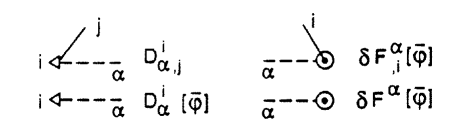
Figure 2: Additional Feynman rules for $\delta X^{j}[\bar{\varphi}]$ in the case of linear gauge generators $D$ and linear gauge fixing $F$

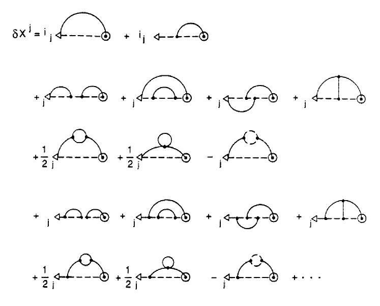
Figure 3: Primary diagram expansion of $\delta X^{j}[\bar{\varphi}]$ through 2-loop order. Contributions involving an undifferentiated $\delta F^{\alpha}[\bar{\varphi}]$ have been dropped, which corresponds to omitting the trivial tree-level gauge dependence Kobes:1991dc

The diagrammatic content of (72) is more conveniently investigated after a Legendre transformation of $W[J]\equiv-i\ln Z[J]$ to the effective action

$$\Gamma[\bar{\varphi}]=W[J]-J_{j}\bar{\varphi}^{j},\qquad\bar{\varphi}^{j}={\delta W[J]\over\delta J_{j}},$$ (73)

which is the generating functional of one-particle-irreducible (1-p-i) diagrams. Equation (72) then becomes

$$\delta\Gamma[\bar{\varphi}]={\delta\Gamma[\bar{\varphi}]\over\delta\bar{\varphi}^{j}}\left\langle D^{j}_{\alpha}[\varphi]\mathscr{G}^{\alpha}{}_{\beta}[\varphi]\,\delta F^{\beta}[\varphi]\right\rangle[\bar{\varphi}]\equiv\Gamma_{,j}[\bar{\varphi}]\,\delta X^{j}[\bar{\varphi}]\;.$$ (74)

Diagrammatically, $\Gamma_{,j}[\bar{\varphi}]$ is the sum of all mean-field dependent (primary) 1-p-i one-point diagrams, while $\delta X^{j}[\bar{\varphi}]$ is given by primary diagrams which involve the additional vertices introduced in Fig. 2 and which are 1-p-i except for the basic ghost line attached to $\delta F^{\beta}$, as shown in Fig. 3.

From these relations one can derive gauge dependence identities for 1-p-i vertex functions by differentiation with respect to $\bar{\varphi}$. For example, the gauge dependences of the 2-point vertex function (self-energy) $\Gamma_{,ij}[0]$ are determined by the diagrams shown in Fig. 4.

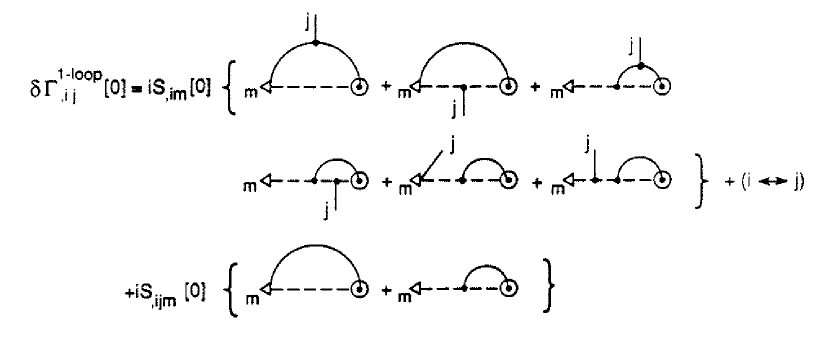
Figure 4: Gauge dependence of the 2-point vertex function $\Gamma_{ij}[0]$ assuming that all one-point functions vanish at $\bar{\varphi}=0$

QED

As a first application let us consider the case of an Abelian theory such as QED. The additional Feynman rules of Fig. 2 involve the ghost propagator, but there are no further ghost vertices in the theory (for linear gauge fixing), so only the very first diagram in Fig. 4 arises.

Furthermore, the structure of the gauge generator is such that

$$\raisebox{-5.0pt}[0.0pt][0.0pt]{\includegraphics[width=39.0242pt]{Dia-.ps}}=\left\{\begin{array}[]{ll}\partial_{\mu_{i}}^{(x_{i})}&\mbox{if $i\leftrightarrow A_{\mu_{i}}(x_{i})$}\\ 0&\mbox{else}\end{array}\right.\;\raisebox{-9.0pt}[0.0pt][0.0pt]{\includegraphics[width=39.0242pt]{Diaj-.ps}}=\left\{\begin{array}[]{ll}0&\mbox{if $i,j\leftrightarrow A_{\mu}$}\\ \pm\mathrm{i}e&\mbox{if $i,j\leftrightarrow\stackrel{{\scriptstyle(-)}}{{\psi}}$}\end{array}\right.$$ (75)

If the external indices $i,j$ of $\delta\Gamma_{,ij}$ correspond to photons, one finds that one cannot even build the one remaining diagram of Fig. 4, so $\delta\Gamma_{A^{\mu}A^{\nu}}$ proves to be completely gauge-fixing independent. This is in fact a well-known result which can be understood also by the gauge invariance of the electromagnetic current operator.

On the other hand, if the external lines are fermionic, there is a non-trivial right-hand-side to Fig. 4, as shown in Fig. 5, so the fermion self-energy is a gauge fixing dependent quantity, already in QED.

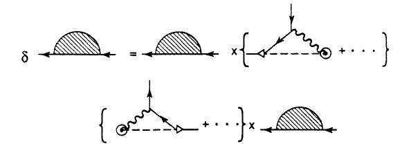
Figure 5: Gauge dependence identity for the fermion self-energy

Hard Thermal/Dense Loops

In the high-temperature (large-chemical-potential) limit of QED and QCD, it turns out that the leading contributions to the 1-loop vertex functions, the so-called “hard thermal (dense) loops” (HTL/HDL) obey tree-level-type ghost-free Ward identities and appear to be gauge-fixing independent Frenkel:1990br ; Braaten:1990mz ; Braaten:1990az . This gauge independence, however, does not arise in an obvious way and involves non-trivial cancellations in the various gauges that have been considered.

The above gauge dependence identities can be used to verify the gauge independence of the HTL’s in a rather simple manner. The only further ingredients needed are the temperature power-counting rules given in Braaten:1990mz , which, roughly, read as follows: in a Feynman diagram, explicit loop momenta in the numerator give a factor $T$, each propagator counts as $T^{-1}$, and the sum-integral over the loop momentum contributes $T^{3}$ unless there are two or more propagators with the same statistics, in which case the sum-integral counts as $T^{2}$.

By this, the leading temperature contributions to a 1-loop vertex function are found to be proportional to $T^{2}$, such that an $N$-point gluon vertex function scales as $\Gamma_{,(N)}\sim g^{N}T^{2}k^{2-N}$ (where $k$ represents generically components of external momenta). If two external lines are fermionic, we have $\Gamma_{,(N)}\sim g^{N}T^{2}k^{1-N}$, while vertex functions with more than two external fermion lines do not contribute terms $\propto T^{2}$.

Considering e.g. vertex functions with only external gluons, all of the potential gauge dependences of the HTL’s are contained in the 1-loop contributions to $\delta\Gamma_{,(N)}=\sum\limits_{M=0\atop perms.}^{N}\Gamma_{,(N+1-M)}\delta X^{\cdot}_{,(M)}$ with the diagrammatic structure of $\delta X^{\cdot}_{,(M)}$ as given by

$$\delta X^{\cdot}_{,(M)}=\sum_{\rm perm.}\biggl{\{}\;\;\raisebox{-38.0pt}{\includegraphics[width=216.81pt]{dxin-.ps}}\biggr{\}}$$ (76)

The above temperature power-counting rules are modified only by the additional vertex $\delta F^{\alpha}_{,i}[0]$ which may bring in one power of loop momentum and thus one power of $T$ in derivative gauges, or none in algebraic ones. Adding up, one finds that the right-hand-side of (76) is proportional to $T^{0\ldots 1}$. Hence, gauge dependences of one-loop vertex functions can occur only at subleading order $\propto T$. HTL(HDL)’s on the other hand are found to be completely gauge-fixing independent.

5.3 Gauge Independence of Propagator Singularities

In non-Abelian gauge theories, all the matter and gauge field vertex functions, self-energies, and propagators contain highly nontrivial gauge dependences, which raises the question whether there is any gauge-independent and therefore potentially physical information in those at all. We shall give an affirmative answer by showing that (the locations of) certain singularities of the full propagators are indeed gauge independent Kobes:1990xf .

Non-Abelian Gauge-Boson Propagator

We begin by analysing the Lorentz structure of the gluon propagator in the case of a general gauge that preserves the rotational symmetry. Moreover, we shall simplify things by dropping any color indices, which presupposes the absence of color symmetry breaking.

In momentum space one can define a transverse projection of the 4-velocity of the heat bath, $\tilde{n}^{\mu}=(g^{\mu\sigma}-{k^{\mu}k^{\sigma}\over k^{2}})u_{\sigma}$, and use it to write the general structure of the gauge-boson propagator as

$$G^{\mu\nu}(k)=\Delta_{A}\mathscr{A}^{\mu\nu}+\Delta_{B}\mathscr{B}^{\mu\nu}+\Delta_{C}\mathscr{C}^{\mu\nu}+\Delta_{D}\mathscr{D}^{\mu\nu}$$ (77)

with

$$\begin{array}[]{l@{\qquad}l}\displaystyle\mathscr{A}^{\mu\nu}(k)=[g^{\mu\nu}-{k^{\mu}k^{\nu}\over k^{2}}]-{\tilde{n}^{\mu}\tilde{n}^{\nu}\over\tilde{n}^{2}}\,,&\displaystyle\mathscr{B}^{\mu\nu}(k)={\tilde{n}^{\mu}\tilde{n}^{\nu}\over\tilde{n}^{2}}\,,\\[8.0pt] \displaystyle\mathscr{C}^{\mu\nu}(k)={1\over|{\vec{k}}|}\left\{\tilde{n}^{\mu}k^{\nu}+k^{\mu}\tilde{n}^{\nu}\right\}\,,&\displaystyle\mathscr{D}^{\mu\nu}(k)={k^{\mu}k^{\nu}\over k^{2}}\,.\end{array}$$ (78)

Here $\mathscr{A}^{\mu\nu}$ is the spatially transverse projector introduced already in (56), and $\mathscr{B}^{\mu\nu}$ is a second, independent tensor that is likewise transverse with respect to 4-momentum, but longitudinal with respect to 3-momentum. $\mathscr{C}^{\mu\nu}$ and $\mathscr{D}^{\mu\nu}$ complete the basis of symmetric tensors, with $\mathscr{C}^{\mu\nu}$ chosen such that $k_{\mu}\mathscr{C}^{\mu\nu}k_{\nu}=0$, and $\mathscr{D}^{\mu\nu}$ longitudinal with respect to 4-momentum.

$\mathscr{A}$, $\mathscr{B}$, and $\mathscr{D}$ are idempotent, whereas $\mathscr{C}^{2}=-(\mathscr{B}+\mathscr{D})$. Under a Lorentz trace, products of one such tensor with a different one vanish; without trace, $\mathscr{A}$ is orthogonal to all the others, but among the rest one only has $\mathscr{B}\perp D$.

Similarly, we shall decompose the gluon self-energy $\Pi^{\mu\nu}={G}^{-1{\mu\nu}}-{G}^{-1{\mu\nu}}_{0}$ according to

$$\Pi^{\mu\nu}=-\Pi_{A}\mathscr{A}^{\mu\nu}-\Pi_{B}\mathscr{B}^{\mu\nu}-\Pi_{C}\mathscr{C}^{\mu\nu}-\Pi_{D}\mathscr{D}^{\mu\nu}\;.$$ (79)

At momentum scales $\omega,k\ll T,\mu$, the leading-order term in the one-loop polarisation tensor $\Pi^{\mu\nu}$ is given by the HTL (HDL) $\sim{\rm max}(T^{2},\mu^{2})$, which has only 4-d-transverse contributions

$$\halign to=433.62pt{\@eqnsel\hskip\@centering$\displaystyle{#}$&\global\@eqcnt\@ne\hskip 2\arraycolsep\hfil${#}$\hfil&\global\@eqcnt\tw@\hskip 2\arraycolsep$\displaystyle{#}$\hfil&\llap{#}\cr 0.0pt plus 1000.0pt$\displaystyle{\Pi_{A}^{\rm HTL} &10.0pt\hfil${=&10.0pt$\displaystyle{{1\over 2} (\Pi^{\rm HTL}{}_{\mu}{}{}^{\mu}- \Pi^{\rm HTL}_{B}){}&\hbox to0.0pt{\hss{\rm(0.80a)}\cr\penalty 100\vskip 3.0pt\vskip 0.0pt\cr 0.0pt plus 1000.0pt$\displaystyle{\Pi_{B}^{\rm HTL} &10.0pt\hfil${=&10.0pt$\displaystyle{-{k^{2}\over{\vec{k}}^{2}} \Pi^{\rm HTL}_{00}{}&\hbox to0.0pt{\hss{\rm(0.80b)}\cr\penalty 100\vskip 3.0pt\vskip 0.0pt\cr 0.0pt plus 1000.0pt$\displaystyle{\Pi_{C}^{\rm HTL} &10.0pt\hfil${=&10.0pt$\displaystyle{0{}&\hbox to0.0pt{\hss{\rm(0.80c)}\cr\penalty 100\vskip 3.0pt\vskip 0.0pt\cr 0.0pt plus 1000.0pt$\displaystyle{\Pi_{D}^{\rm HTL} &10.0pt\hfil${=&10.0pt$\displaystyle{0 &\hbox to0.0pt{\hss{\rm(0.80d)}\cr}}}}}}}}}}}}}}}}}$$

where, at high $T$,

$$\Pi^{\rm HTL}{}_{\mu}{}{}^{\mu}={{e^{2}T^{2}}\over 3},$$ (81)

$$\Pi^{\rm HTL}_{00}={{e^{2}T^{2}}\over 3}\left(1-{k^{0}\over 2|{\vec{k}}|}\ln{k^{0}+|{\vec{k}}|\over k^{0}-|{\vec{k}}|}\right).$$ (82)

As a function of frequency and 3-momentum, the result is identical in QED and QCD, if for the latter we define $e^{2}:=g^{2}(N+N_{f}/2)$ (for ${\rm SU}(N)$ with $N_{f}$ flavors) Kalashnikov:1980cy ; Weldon:1982aq . If there is also a nonvanishing chemical potential $\mu$, a similar result holds where $T^{2}\to T^{2}+{3\over\pi^{2}}\mu^{2}$ in terms $\propto N_{f}$ (all of them in QED)—with obvious generalization to the case of different chemical potentials $\mu_{i}$ for different flavors $i$.

The HTL-dressed propagator $G^{\rm HTL}=(G_{0}^{-1}+\Pi^{\rm HTL})^{-1}$ has poles off the usual light-cone, which come in two branches determined by

$$\halign to=433.62pt{\@eqnsel\hskip\@centering$\displaystyle{#}$&\global\@eqcnt\@ne\hskip 2\arraycolsep\hfil${#}$\hfil&\global\@eqcnt\tw@\hskip 2\arraycolsep$\displaystyle{#}$\hfil&\llap{#}\cr 0.0pt plus 1000.0pt$\displaystyle{\Delta_{A}^{\rm HTL-1}&10.0pt\hfil${=&10.0pt$\displaystyle{k^{2} - \Pi_{A}^{\rm HTL}=0{}&\hbox to0.0pt{\hss{\rm(0.83a)}\cr\penalty 100\vskip 3.0pt\vskip 0.0pt\cr 0.0pt plus 1000.0pt$\displaystyle{\Delta_{B}^{\rm HTL-1}&10.0pt\hfil${=&10.0pt$\displaystyle{k^{2} - \Pi_{B}^{\rm HTL}=0 &\hbox to0.0pt{\hss{\rm(0.83b)}\cr}}}}}}}}}$$

Since, as we have seen above, the HTL contribution is completely gauge independent and the gauge fixing parameters contained in $G_{0}^{-1}$ do not appear in (5.3,5.3), the $A$- as well as the $B$-part of the HTL propagator is completely gauge independent.

The physical interpretation of the $A$- and $B$-branch of propagator poles (displayed in Fig. 6) is that the former represents quasi-particles which are in-medium versions of the physical polarisation of the gauge bosons, while the appearance of the $B$-branch is a purely collective phenomenon corresponding to charge density oscillations (plasmons) above the plasma frequency and to charge screening below.

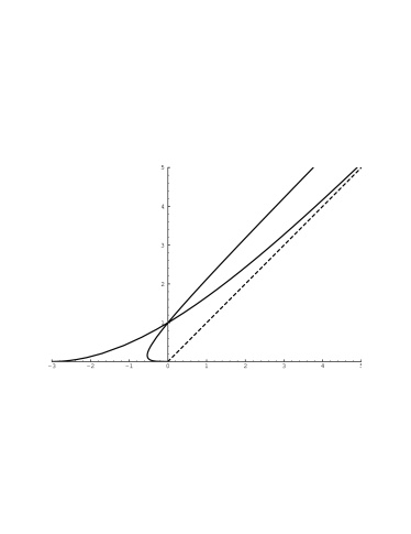
Figure 6: The location of the zeros of $\Delta_{A}^{{\rm HTL}-1}$ (transverse gluons) and of $\Delta_{B}^{{\rm HTL}-1}$ (longitudinal plasmons) in quadratic scales such as to show propagating modes and screening phenomena on one plot. Above a common plasma frequency $\omega_{\rm pl.}$ there are propagating quasi-particle modes, which for large momenta in branch A tend to a mass hyperboloid with asymptotic mass $m_{\infty}^{2}={3\over 2}\omega_{\rm pl.}^{2}$, and in branch B approach the light-cone exponentially with exponentially vanishing residue. For $\omega<\omega_{\rm pl.}$, $|\mathbf{k}|$ is the inverse screening length, which in the static limit vanishes for mode A (absence of magnetostatic screening), but reaches the Debye mass, $\hat{m}_{D}^{2}=3\omega_{\rm pl.}^{2}$, for mode B (electrostatic screening)

Beyond the HTL approximation and in non-Abelian theories, however, one has gauge parameter dependences within $\Pi$, and also $\Pi_{\mu\nu}k^{\mu}\not=0$ so that $\Pi_{C}\not=0,\Pi_{D}\not=0$.

Considering a general, rotationally invariant gauge $\tilde{f}^{\mu}(k)\tilde{A}_{\mu}(k)$ as in (54), this can be parameterized as

$$\tilde{f}^{\mu}(k)=\tilde{\beta}(k)k^{\mu}+\tilde{\gamma}(k)\tilde{n}^{\mu}.$$ (84)

Covariant gauges then correspond to $\tilde{\beta}=1,\tilde{\gamma}=0$, Coulomb gauges to $\tilde{\beta}=\tilde{n}^{2},\tilde{\gamma}=-k^{0}$, and temporal axial gauge to $\tilde{\beta}=k^{0}/k^{2},\tilde{\gamma}=1$.

The structure functions of the gauge propagator become more complicated, to wit,

$$\halign to=433.62pt{\@eqnsel\hskip\@centering$\displaystyle{#}$&\global\@eqcnt\@ne\hskip 2\arraycolsep\hfil${#}$\hfil&\global\@eqcnt\tw@\hskip 2\arraycolsep$\displaystyle{#}$\hfil&\llap{#}\cr 0.0pt plus 1000.0pt$\displaystyle{\Delta_{A} &10.0pt\hfil${=&10.0pt$\displaystyle{[ k^{2} - \Pi_{A} ]^{-1} {}&\hbox to0.0pt{\hss{\rm(0.85a)}\cr\penalty 100\vskip 3.0pt\vskip 0.0pt\cr 0.0pt plus 1000.0pt$\displaystyle{\Delta_{B} &10.0pt\hfil${=&10.0pt$\displaystyle{[ k^{2} - \Pi_{B} - {2\tilde{\beta}\tilde{\gamma}|{\vec{k}}| \Pi_{C} - \alpha\Pi_{C}^{2} + \tilde{\gamma}^{2} {\tilde{n}}^{2} \Pi_{D} \over\tilde{\beta}^{2} k^{2} - \alpha\Pi_{D} } ]^{-1} {}&\hbox to0.0pt{\hss{\rm(0.85b)}\cr\penalty 100\vskip 3.0pt\vskip 0.0pt\cr 0.0pt plus 1000.0pt$\displaystyle{\Delta_{C} &10.0pt\hfil${=&10.0pt$\displaystyle{-{\tilde{\beta}\tilde{\gamma}|{\vec{k}}| - \alpha\Pi_{C} \over\tilde{\beta}^{2} k^{2} - \alpha\Pi_{D}} {}&\hbox to0.0pt{\hss{\rm(0.85c)}\cr\penalty 100\vskip 3.0pt\vskip 0.0pt\cr 0.0pt plus 1000.0pt$\displaystyle{\Delta_{D} &10.0pt\hfil${=&10.0pt$\displaystyle{{ \tilde{\gamma}^{2} \tilde{n}^{2} + \alpha(k^{2}-\Pi_{B}) \over\tilde{\beta}^{2} k^{2} - \alpha\Pi_{D} } \Delta_{B} &\hbox to0.0pt{\hss{\rm(0.85d)}\cr}}}}}}}}}}}}}}}}}$$

and there are gauge parameters everywhere, both explicitly and also within the structure functions of $\Pi$.

These gauge dependences are controlled by the gauge dependence identities discussed above, and, in compact notation, they have the form

$$\delta\Delta^{ij}\Big{|}_{J=0}=-(\Delta^{im}\delta X^{j}_{,m}+\delta X^{i}_{,m}\Delta^{mj})\Big{|}_{J=0}$$ (86)

for the full propagator. Specialized to the thermal gauge-boson propagator in $f^{\mu}$-gauge, one finds Kobes:1990xf ; Kobes:1991dc

$$\halign to=433.62pt{\@eqnsel\hskip\@centering$\displaystyle{#}$&\global\@eqcnt\@ne\hskip 2\arraycolsep\hfil${#}$\hfil&\global\@eqcnt\tw@\hskip 2\arraycolsep$\displaystyle{#}$\hfil&\llap{#}\cr 0.0pt plus 1000.0pt$\displaystyle{\delta{ \Delta_{A}^{-1}}&10.0pt\hfil${=&10.0pt$\displaystyle{{ \Delta_{A}^{-1}}\Bigl{[}-\mathscr{A}^{\mu}_{\nu}(k)\delta X^{\nu}_{,\mu}(k)\Bigr{]} \equiv{ \Delta_{A}^{-1}}\delta Y {}&\hbox to0.0pt{\hss{\rm(0.87a)}\cr\penalty 100\vskip 3.0pt\vskip 0.0pt\cr 0.0pt plus 1000.0pt$\displaystyle{\delta{ \Delta_{B}^{-1}} &10.0pt\hfil${=&10.0pt$\displaystyle{{ \Delta_{B}^{-1}} \left[-{\tilde{n}^{\mu}\over\tilde{n}^{2}}+ {\tilde{\gamma}\tilde{\beta}-\alpha\Pi_{C}/|\vec{k}| \over\tilde{\beta}^{2} k^{2} -\alpha\Pi_{D}}k^{\mu}\right]2\tilde{n}_{\nu}\delta X^{\nu}_{,\mu} \equiv{ \Delta_{B}^{-1}}\delta Z &\hbox to0.0pt{\hss{\rm(0.87b)}\cr}}}}}}}}}$$

but no such relations for $\Delta_{C}$ and $\Delta_{D}$.

If $\delta Y$ and $\delta Z$ are regular on the two “mass-shells” defined by $\Delta_{A}^{-1}=0$ and $\Delta_{B}^{-1}=0$, the relations (5.3,5.3) imply that the locations of these particular singularities of the gluon propagator are gauge fixing independent, for if $\Delta_{A}^{-1}=0=\Delta_{B}^{-1}$ then also $\Delta_{A}^{-1}+\delta\Delta_{A}^{-1}=0=\Delta_{B}^{-1}+\delta\Delta_{B}^{-1}$.

So everything depends on whether the possible singularities of $\delta X^{\nu}_{,\mu}$ could coincide with the expectedly physical dispersion laws $\Delta_{A}^{-1}=0$ and $\Delta_{B}^{-1}=0$. Diagrammatically, $\delta X^{\nu}_{,\mu}$ is obtained from the primary diagrams of Fig. 3 by inserting one additional vertex in all possible ways (and omitting all resulting tadpole-like diagrams in the case of no spontaneous symmetry breaking). Since the primary diagrams are 1-particle reducible with respect to the basic ghost line attached to $\delta F^{\alpha}_{i}$, $\delta X^{\nu}_{,\mu}$ will have singularities like the (full) ghost propagator. These singularities are however generically different from those that define the spatially transverse and longitudinal gauge-boson quasi-particles. Indeed, in leading-order thermal perturbation theory, the temperature power-counting rules referred to in Sect. 5.2 imply that the ghost propagator does not receive contributions $\sim e^{2}T^{2}$ and thus will have completely different dispersion laws.

The other parts of the diagrams making up $\delta X^{\nu}_{,\mu}$ are 1-p-i and may develop singularities for other reasons, namely when one line of such an 1-p-i diagram is of the same type as the external one, and the remaining ones are massless. This may potentially give rise to infrared or mass-shell singularities. However, these singularities will be absent as soon as an overall infrared cut-off is introduced, for example by considering first a finite volume. In every finite volume, this obstruction to the gauge-independence proof is then avoided, and $\Delta_{A}^{-1}=0$ and $\Delta_{B}^{-1}=0$ define gauge-independent dispersion laws if the infinite volume limit is taken last of all Rebhan:1992ak .

This reasoning leads to the conclusion that the positions of all the singularities of $\Delta_{A}$ are gauge-fixing independent, though not necessarily their type or e.g. their residues if they are simple poles. In the case of $\Delta_{B}$, there is a slight complication by the contents of the square bracket in (5.3). There is a kinematical pole $1/k^{2}$ hidden in the $\tilde{n}$’s, and there is a contribution from the obviously gauge-dependent $\Delta_{D}$ (cf. (5.3)). These gauge artefacts have to be excluded, but they are gauge dependent already at tree level and thus easy to identify. For example, $\Delta_{B}$ as defined above has a factor of $k^{2}$ which cancels in the Coulomb gauge propagator but not in that of covariant gauges, so this massless mode is a gauge mode and thus unphysical.

The gauge-(in)dependence identities (5.3,5.3) also explain the gauge dependences found in the one-loop calculation of the plasmon damping constant mentioned above. Truncating e.g. (5.3) at one-loop order gives

$$\delta{\Delta_{A}^{-1}{}^{(1)}}(k)={\Delta_{A}^{-1}{}^{(0)}}\delta Y^{(1)},$$ (88)

with superscripts referring to bare loop order and using that $\delta Y^{(0)}\equiv 0$. However, the HTL plasma dispersion law is derived from $\Delta_{A}^{-1}{}^{(0)}+\Delta_{A}^{-1}{}^{(1)}=0$, and the “correction” $\Delta_{A}^{-1}{}^{(1)}\sim\Pi^{\rm HTL}\sim g^{2}T^{2}\sim\omega_{\rm pl.}^{2}$ is not small but sets the scale for everything. The temperature-power-counting rules of Sect. 5.2 give $\delta Y^{(1)}\sim g^{2}T/\omega_{\rm pl.}$, so the right-hand side of (88) does not vanish at the order of the damping contribution $\gamma\times\omega_{\rm pl.}\sim g\omega_{\rm pl.}^{2}$.

On the other hand, if one does have a good expansion parameter (which bare loop order obviously is not), then the identities (5.3,5.3) imply order-by-order gauge independence.

As will be discussed further below, HTL perturbation theory Braaten:1990kk ; Braaten:1990mz claims to be a systematic framework, although not up to arbitrarily high orders, and the expansion parameter is essentially $\sqrt{g^{2}}$. In Braaten:1990it , the long-wavelength plasmon damping constant has been calculated by Braaten and Pisarski with the result $\gamma(|\vec{k}|=0)/[{g^{2}TN\over 24\pi}]=+6.635\ldots$ and formal checks as to its gauge independence were positive.

More explicit calculations by Baier et al., however, revealed that, in covariant gauges and on plasmon-mass-shell, HTL-resummed perturbation theory still leads to explicit gauge dependent contributions to the damping of fermionic Baier:1992dy as well as gluonic Baier:1992mg quasi-particles. But, as was pointed out in Rebhan:1992ak , these apparent gauge dependences are avoided if the quasi-particle mass-shell is approached with a general infrared cut-off such as finite volume, and this cut-off lifted only in the end. This procedure defines gauge-independent dispersion laws and the gauge dependent parts are found to pertain to the residue, which at finite temperature happens to be linearly infrared singular in covariant gauges, rather than only logarithmically as at zero temperature, due to Bose enhancement.

Extension to Fermions

The fermion propagator at non-zero temperature or density has one more structure function than usually. In the ultrarelativistic limit where masses can be neglected, the fermion self-energy can be parametrized according to

$$\Sigma(k_{0},{\vec{k}})\,=\,a(k_{0},k)\,\gamma^{0}\,+\,b(k_{0},k){\hat{\vec{k}}}\cdot\boldsymbol{\gamma}$$ (89)

with $\hat{\vec{k}}=\vec{k}/|\vec{k}|$ (again neglecting the possibility of color superconductivity).

Defining $\Sigma_{\pm}(k_{0},k)\equiv b(k_{0},k)\pm\,a(k_{0},k)$, a natural decomposition of the fermion self-energy and propagator $S^{-1}=-{\not\!k}+\Sigma$ is given by

$$\gamma_{0}\Sigma(k_{0},{\bf k}) = \Sigma_{+}(k_{0},k)\Lambda_{+}(\hat{\vec{k}})\,-\,\Sigma_{-}(k_{0},k)\Lambda_{-}(\hat{\vec{k}}),$$ (90)

$$\gamma_{0}S^{-1}(k_{0},{\bf k}) = \Delta_{+}^{-1}(k_{0},k)\Lambda_{+}(\hat{\vec{k}})\,+\,\Delta_{-}^{-1}(k_{0},k)\Lambda_{-}(\hat{\vec{k}})$$ (91)

with $\Delta_{\pm}^{-1}\equiv-[k_{0}\mp(k+\Sigma_{\pm})]$ and spin matrices

$$\Lambda_{\pm}(\hat{\vec{k}}) \equiv \frac{1\pm\gamma^{0}\boldsymbol{\gamma}\cdot\hat{\vec{k}}}{2},\qquad\Lambda_{+}+\Lambda_{-}=1,$$ (92)

$$\Lambda_{\pm}^{2} = \Lambda_{\pm},\qquad\Lambda_{+}\Lambda_{-}\,=\,\Lambda_{-}\Lambda_{+}=0,\qquad{\rm Tr}\Lambda_{\pm}=2,$$ (93)

projecting onto spinors whose chirality is equal ($\Lambda_{+}$), or opposite ($\Lambda_{-}$), to their helicity.

In the HTL approximation where $|k_{0}|,|{\bf k}|\ll{\rm max}(T,\mu)$, the fermion self-energy has been first calculated by Klimov Klimov:1981ka as

$$\Sigma^{\rm HTL}_{\pm}(k_{0},k)\,=\,{\hat{M}^{2}\over k}\,\left(1\,-\,\frac{k_{0}\mp k}{2k}\,\log\,\frac{k_{0}+k}{k_{0}-k}\right)$$ (94)

where $\hat{M}^{2}$ is the plasma frequency for fermions, i.e., the frequency of long-wavelength ($k\to 0$) fermionic excitations

$$\hat{M}^{2}={g^{2}C_{f}\over 8}\left(T^{2}+{\mu^{2}\over\pi^{2}}\right).$$ (95)

($C_{f}=(N^{2}-1)/2N$ in SU($N$) gauge theory, and $g^{2}C_{f}\to e^{2}$ in QED.)

This leads to two separate branches of dispersion laws of fermionic quasi-particles $\Delta_{\pm}(\omega,k)^{-1}=0$ carrying particle and hole quantum numbers respectively Weldon:1989ys ; Pisarski:1989wb . As shown in Fig. 7, the $(-)$-branch, which is occasionally nicknamed “plasmino”, exhibits a curious dip reminiscent of the dispersion law of rotons in liquid helium.

Figure 7: The location of the zeros of $\Delta_{\pm}^{-1}$ in the HTL approximation in quadratic scales. The additional collective modes of branch $(-)$ (“plasminos”) has a minimum of $\omega$ at $\omega/\hat{M}\approx 0.93$ and $|\vec{k}|/\hat{M}\approx 0.41$ and approaches the light-cone for large momenta, but with exponentially vanishing residue. The regular branch approaches a mass hyperboloid (here a straight line parallel to the diagonal) with asymptotic mass $\sqrt{2}\hat{M}$

As we have seen in Sect. 5.2, gauge dependences start at order $T$ in the high-temperature expansion. While the HTL result (94) is completely gauge independent, gauge parameter dependences enter at subleading order. The gauge dependence identity for the fermion propagator is, however, somewhat simpler than that for the gluon propagator. The singularities in the fermion propagator can be summarized by

$$\det\!\left(S^{-1}_{\sigma\bar{\varrho}}\right)=0$$ (96)

where $\sigma,\bar{\varrho}$ are spinor indices. The gauge dependence identity thus takes the form

$$\delta\det\left(S^{-1}_{\sigma\bar{\varrho}}\right)\!(k)=-\det\left(S^{-1}_{\sigma\bar{\varrho}}\right)\!(k)\,[\delta X^{\tau}_{,\tau}(k)+\delta X^{\bar{\tau}}_{,\bar{\tau}}(k)]$$ (97)

where the two expressions within the square brackets are Dirac traces of the diagrams appearing within the braces in Fig. 5.

The conclusion of gauge independence of the solutions of (96) can now be reached by essentially the same arguments as those for the gauge boson propagator (with the exception that now there are no additional, gauge-dependent kinematical poles like those arising in the projection onto mode $B$ in (5.3)). The only obstruction to gauge independence comes from singularities of $\delta X^{\tau}_{,\tau}(k)$ and $\delta X^{\bar{\tau}}_{,\bar{\tau}}(k)$. If mass-shell singularities from massless gauge modes are avoided by infrared regularization or finite volume, only the singularities of the ghost propagator need to be considered. Again, the latter are generically different from those leading to the now fermionic quasi-particles since ghosts do not have HTL self-energies $\sim T^{2}$.

We have thus seen that all the singularities of the fermion propagator as well as those of the $A$- and $B$-branch of the gluon propagator (with some exceptions for the latter) are gauge-fixing independent. On the other hand, residues (if those singularities are simple poles at all) are not protected and may be gauge dependent; even the nature of the singularity may be different from gauge to gauge, as is well known to be the case already for the electron propagator in zero-temperature QED BogS:QF .

6 Quasiparticles in HTL Perturbation Theory

We have already seen that loop order in bare perturbation theory is not a good expansion parameter for calculating corrections to quasi-particle properties at soft scales $\sim gT$. Technically what happens is that the HTL contributions to one-loop vertex functions are of the same order of magnitude as their tree-level counterparts for external momenta $k\sim gT$:

$$\quad{\Gamma_{,N}^{\rm HTL}}\sim g^{N}{T^{2}}{k^{2-N}}\sim g^{N-2}{k^{4-N}}\sim{\partial^{N}\mathcal{L}\over\partial A^{N}}\Big{|}_{k\sim gT}.$$ (98)

Therefore all HTL contributions need to be resummed in Feynman diagrams that are sensitive to the soft regime $k\sim gT$.

Since HTL’s are the leading contributions from hard momenta $k\sim T$, this can be understood as the transition from the bare Lagrangian to an effective, Wilson-renormalized one for $k\sim gT$, $\mathcal{L}\to\mathcal{L}+\mathcal{L}^{\rm HTL}$. $\mathcal{L}^{\rm HTL}$ is the effective Lagrangian containing all the HTL diagrams and arises from integrating out all hard modes.

Soon after the identification of all the HTL’s of QCD in Frenkel:1990br ; Braaten:1990mz , it has been found that, formally, $\mathcal{L}^{\rm HTL}$ has a comparatively simple and manifestly gauge-invariant integral representation Taylor:1990ia ; Braaten:1992gm ; Frenkel:1992ts

$$\mathcal{L}^{\rm HTL} = \hat{M}^{2}\int{d\Omega_{v}\over 4\pi}\bar{\psi}\gamma^{\mu}{{v_{\mu}}\over{v}\cdot D(A)}\psi$$ (100)

$$-{3\over 2}\omega^{2}_{pl.}{\rm tr}\int{d\Omega_{v}\over 4\pi}F^{\mu\alpha}{{v_{\alpha}}{v^{\beta}}\over({v}\cdot D_{adj.}(A))^{2}}F_{\mu\beta}$$

with $\hat{M}^{2}$ the fermionic plasma frequency given in (95) and $\omega^{2}_{pl.}=\frac{1}{3}\Pi^{\rm HTL}_{\mu}{}^{\mu}$ the more familiar one of the gauge bosons (cf. (81)). In this integral representation $v=(1,\vec{v})$ is a light-like 4-vector, i.e. with $\vec{v}^{2}=1$, and its spatial components are averaged over by $d\Omega_{v}$. $v$ is the remnant of the hard plasma constituents’ momenta $p^{\mu}\sim Tv^{\mu}$, namely their light-like 4-velocity, and the overall scale $T$ has combined with the coupling constant to form the scale of thermal masses, $\hat{M},\omega_{pl.}\sim gT$.

The HTL effective Lagrangian (100) is manifestly gauge invariant and moreover gauge independent ($\hat{M}$ and $\omega_{pl.}$ do not depend on the gauge fixing parameters used to integrate out the hard modes). It is non-local and Hermitian only in a Euclidean form, i.e. prior to analytic continuation to real time/frequencies. It has cuts which physically correspond to the phenomenon of Landau damping. The equations of motions associated with (100) can also be obtained from kinetic theory, which is extremely useful to gain further physical insight Blaizot:1993zk ; Blaizot:1994be ; Kelly:1994dh ; Blaizot:2001nr . There is also a noteworthy connection to Chern-Simons theory Efraty:1992gk ; Efraty:1993pd ; Nair:1993rx .

Using (100) as an effective theory for soft scales $\sim gT$ means that the bare propagators are to be replace by those of HTL quasi-particles, and these have infinitely many nonlocal vertices. E.g., the three-gluon vertex becomes

$${\Gamma^{abc}_{\mu\nu\varrho}}^{\rm cl+HTL}(k,q,r) = {\rm i}gf^{abc}\Bigl{\{}g_{\mu\nu}(k-q)_{\varrho}+{\rm cycl.}$$ (101)

$$+ 3\omega^{2}_{\rm pl.}\int{d\Omega_{v}\over 4\pi}v_{\mu}v_{\nu}v_{\varrho}\left[{r_{0}\over k\cdot v\,r\cdot v}-{q_{0}\over k\cdot v\,q\cdot v}\right]\Bigr{\}}.$$ (102)

In QCD, there are HTL vertices for any number of external gluons and up to two quark lines, whereas in QED, where $v\cdot D_{\rm adj.}(A))\to v\cdot\partial$ in (100), there is “only” an HTL photon self-energy $\Pi_{\mu\nu}$, an HTL fermion self-energy $\Sigma$, and vertices involving two fermions and an arbitrary number of photons.

While the effective Lagrangian (100) is gauge invariant and gauge independent in its entirety, NLO corrections won’t be so. However, as we have seen in the previous section, the positions of singularities of the effective (quasi-particle) propagators are protected against gauge dependences by the identities (5.3), (5.3), and (97).

6.1 Long-Wavelength Plasmon Damping

The first such correction to be calculated by means of the HTL-resummed perturbation theory was the damping rate of long-wavelength plasmons from the shift of the pole of the gluon propagator at $\vec{k}=0$ from $\omega=\omega_{\rm pl.}^{\rm HTL}$ $\to$ $\omega=\omega_{\rm pl.}-{\rm i}\gamma(\vec{k}=0)$ with the result Braaten:1990it

$$\gamma(\vec{k}=0)=+6.635\ldots{g^{2}NT\over 24\pi}=0.264\sqrt{N}{g}\,\omega_{\rm pl.}^{\rm HTL},$$ (103)

implying the existence of weakly damped plasmons for $g\ll 1$.

In QCD, where one is interested in the range $g\sim 1$, one finds that the existence of plasmons as quasi-particles requires that $g$ is significantly less than 2.2, so real QCD is on the borderline of having identifiable long-wavelength quasi-particles.

The corresponding quantity for fermionic quasi-particles has been calculated in Kobes:1992ys ; Braaten:1992gd with a comparable result: weakly damped long-wavelength fermionic quasi-particles in 2- or 3-flavor QCD require that $g$ is significantly less than 2.7.

6.2 NLO Correction to Gluonic Plasma Frequency

In Schulz:1994gf , Schulz has calculated also the real part of the NLO contribution to the gluon polarization tensor in the limit of $\vec{k}\to 0$ which determines the NLO correction to the gluonic plasma frequency.

The original power-counting arguments of Braaten:1990mz suggested that besides one-loop diagrams with HTL-resummed propagators and vertices, there could be also contributions from two-loop diagrams to relative order $g$. The explicit (and lengthy) calculation of Schulz:1994gf showed that those contribute only at order $g^{2}\ln(1/g)$ rather than $g$, and the NLO plasma frequency in a pure-glue plasma was obtained as

$$\omega_{\rm pl.}=\omega_{\rm pl.}^{\rm HTL}\left[1-0.09\sqrt{N}{g}\right].$$ (104)

In this particular result, HTL-resummed perturbation theory turns out to give a moderate correction to the leading-order HTL value even for $g\sim 1$; see however below.

While the calculations leading to (103) and (104) contain some interesting physics, in the following we shall go into more detail only for a couple of more tractable cases, which nonetheless will turn out to involve a number of salient points.

6.3 NLO Correction to the Non-Abelian Debye Mass

The poles of the (gluon) propagator do not only give the dispersion law of quasi-particles, but also the screening of fields with frequencies below the plasma frequency and in particular of static fields. Below the plasma frequency, there are poles for $\vec{k}^{2}<0$, as displayed in Fig. 6, corresponding in configuration space to exponential fall-off with (frequency-dependent) screening mass $\sqrt{|\vec{k}^{2}|}$, i.e. screening length $1/\sqrt{|\vec{k}^{2}|}$.

In the static case, branch $A$ of the gluon propagator describes the screening of (chromo-)magnetostatic fields. While there is a finite screening length as long as $\omega>0$, the $A$-branch of the HTL propagator becomes unscreened in the static limit. Whereas in QED, a “magnetic mass” is forbidden by gauge invariance Fradkin:1965 ; Blaizot:1995kg , some sort of entirely non-perturbative magnetic mass is expected in non-Abelian gauge theories in view of severe infrared problems caused by the self-interactions of magnetostatic gluons Polyakov:1978vu ; Linde:1980ts ; Gross:1981br .

Branch $B$, on the other hand, contains the information about screening of (chromo-)electric fields as generated by static charges (Debye screening). The Debye mass given by the leading-order HTL propagator is $\hat{m}_{D}=\sqrt{3}\omega_{pl.}$. The determination of its NLO correction has a history that is at least as long as the plasmon (damping) puzzle, for it starts already with (ultra-relativistic) QED.

Customarily, the Debye mass (squared) has been defined as the infrared limit $\Pi_{00}(\omega=0,k\to 0)$, which indeed is correct at the HTL level, cf. (5.3) and (82).

In QED, this definition has the advantage of being directly related to a derivative of the thermodynamic pressure, so that the higher-order terms known from the latter determine those of $\Pi_{00}^{\rm QED}(\omega=0,k\to 0)$ through Fradkin:1965 ; Kap:FTFT

$$\Pi_{00}(0,k\to 0)\Big{|}_{\mu=0}=e^{2}{\partial^{2}P\over\partial\mu^{2}}\Big{|}_{\mu=0}={e^{2}T^{2}\over 3}\left(1-{3e^{2}\over 8\pi^{2}}+{\sqrt{3}e^{3}\over 4\pi^{3}}+\ldots\right)$$ (105)

This result is gauge independent because in QED all of $\Pi_{\mu\nu}$ is.

In the case of QCD, there is no such relation. In fact, one expects $\delta m_{D}^{2}/\hat{m}_{D}^{2}$ $\sim g$ rather than $g^{3}$ because of gluonic self-interactions and Bose enhancement. The calculation of this quantity should be much easier than the dynamic ones considered above, because in the static limit the HTL effective action collapses to just the local, bilinear HTL Debye mass term,

$$\mathcal{L}^{\rm HTL}\stackrel{{\scriptstyle\rm static}}{{\longrightarrow}}-{1\over 2}\hat{m}_{D}^{2}{\rm tr}A_{0}^{2}.$$ (106)

This is also gauge invariant, because $A_{0}$ behaves like an adjoint scalar under time-independent gauge transformations. Resummed perturbation theory thus boils down to a resummation of the HTL Debye mass in the electrostatic propagator, which is what had been done already since long Gell-Mann:1957 ; Kap:FTFT .

Using this simple (“ring”) resummation in QCD, one finds however the gauge dependent result Toimela:1985ht

$$\Pi_{00}(0,0)/m_{D}^{2}=1+{\alpha}{N\over 4\pi}\sqrt{6\over 2N+N_{f}}g$$ (107)

where $\alpha$ is the gauge parameter of general covariant gauge (which coincides with general Coulomb gauge in the static limit).

This result was interpreted as meaning that the non-Abelian Debye mass could not be obtained in resummed perturbation theory Nadkarni:1986cz or that one should use a physical gauge instead Kajantie:1985xx ; Kap:FTFT . In particular, temporal axial gauge was put forward, because in this gauge there is, like in QED, a linear relationship between electric field strength correlators and the gauge propagator. However, because static ring resummation clashes with temporal gauge, inconclusive and contradicting results were obtained by different authors Kajantie:1982hu ; Furusawa:1983gb ; Kajantie:1985xx , and in fact one cannot do without vertex resummations if one wants to be consistent there Baier:1994et ; Peigne:1995dn . But be that as it may be, switching to the chromoelectric field strength correlator is not good enough, for it is gauge variant and its infrared limit is equally gauge dependent Rebhan:1994mx .

On the other hand, in view of the gauge dependence identities discussed in the previous section, the gauge dependence of (107) is no longer surprising. Gauge independence can only be expected “on-shell”, which here means $\omega=0$ but $\vec{k}^{2}\to-\hat{m}_{D}^{2}$.

Indeed, the exponential fall-off of the electrostatic propagator is determined by the position of the singularity of $\Delta_{B}(0,k)$, and not simply by its infrared limit. This implies in particular that one should use a different definition of the Debye mass already in QED, despite the gauge independence of (105), namely Rebhan:1993az

$$m^{2}_{D}=\Pi_{00}(0,k)\Big{|}_{\vec{k}^{2}\to-m_{D}^{2}}.$$ (108)

For QED (with massless electrons), the Debye mass is thus not given by (105) but rather as

$$m^{2}_{D} = \Pi_{00}(0,k\to 0)+\bigl{[}\Pi_{00}(0,k)\big{|}_{k^{2}=-m^{2}_{D}}-\Pi_{00}(0,k\to 0)\bigr{]}$$ (109)

$$= {e^{2}T^{2}\over 3}\biggl{(}1-{3e^{2}\over 8\pi^{2}}+{\sqrt{3}e^{3}\over 4\pi^{3}}+\ldots-{e^{2}\over 6\pi^{2}}[\ln{\tilde{\mu}\over\pi T}+\gamma_{E}-{4\over 3}]+\ldots\biggr{)}$$ (110)

where $\tilde{\mu}$ is the renormalization scale of the momentum subtraction scheme, i.e. $\Pi_{\mu\nu}(k^{2}=-\tilde{\mu}^{2})|_{T=0}=0$. Since $de/d\ln\tilde{\mu}=e^{3}/(12\pi^{2})+O(e^{5})$, (110) is a renormalization-group invariant result for the Debye mass in hot QED, which (105) obviously failed to be.

In QCD, where gauge independence is not automatic, the dependence on the gauge fixing parameter $\alpha$ is another indication that (107) is the wrong definition. For (108) we need the full momentum dependence of the correction $\delta\Pi_{00}(k_{0}=0,{\vec{k}})$ to $\Pi^{\rm HTL}_{00}$. Since only the electrostatic mode needs to be dressed, this is not difficult to obtain Rebhan:1993az :

$$\delta\Pi_{00}(k_{0}=0,{\vec{k}}) = \underbrace{\textstyle g\hat{m}_{D}N\sqrt{\frac{6}{2N+N_{f}}}}_{g^{2}T}\int\frac{d^{3-2\varepsilon}p}{(2\pi)^{3-2\varepsilon}}$$ (111)

$$\times \biggl{\{}\frac{1}{{\vec{p}}^{2}+\hat{m}_{D}^{2}}+\frac{1}{{\vec{p}}^{2}}+\frac{4\hat{m}_{D}^{2}-({\vec{k}}^{2}+\hat{m}_{D}^{2})[3+2{\vec{p}}{\vec{k}}/{\vec{p}}^{2}]}{{\vec{p}}^{2}{[(\vec{p}+\vec{k})^{2}+\hat{m}_{D}^{2}]}}$$ (113)

$$+{\alpha}{({\vec{k}}^{2}+\hat{m}_{D}^{2})}\frac{{\vec{p}}^{2}+2{\vec{p}}{\vec{k}}}{{\vec{p}}^{4}{{[(\vec{p}+\vec{k})^{2}+\hat{m}_{D}^{2}]}}}\biggr{\}}.$$

In accordance with the gauge dependence identities, the last term shows that gauge independence holds algebraically for $\vec{k}^{2}=-\hat{m}_{D}^{2}$. On the other hand, on this “screening mass shell”, where the denominator term $[(\vec{p}+\vec{k})^{2}+\hat{m}_{D}^{2}]\to[\vec{p}^{2}+2\vec{p}\vec{k}]$, we encounter IR-singularities. In the $\alpha$-dependent term, they are such that they produce a divergent factor $1/[\vec{k}^{2}+m_{D}^{2}]$ so that the gauge dependences no longer disappear even on-shell. This is, however, the very same problem that had to be solved in the above case of the plasmon damping in covariant gauges. Introducing a temporary infrared cut-off (e.g., finite volume), does not modify the factor $[\vec{k}^{2}+m_{D}^{2}]$ in the numerator but defuses the dangerous denominator. Gauge independence thus holds for all values of this cut-off, which can be sent to zero in the end. The gauge dependences are thereby identified as belonging to the (infrared divergent) residue.

The third term in the curly brackets, however, remains logarithmically singular on-shell as the infrared cut-off is to be removed. In contrast to the $\alpha$-dependent term, closer inspection reveals that these singularities are coming from the massless magnetostatic modes and not from unphysical massless gauge modes.

At HTL level, there is no (chromo-)magnetostatic screening, but, as we have mentioned, one expects some sort of such screening to be generated non-perturbatively in the static sector of hot QCD at the scale $g^{2}T\sim gm_{D}$ Polyakov:1978vu ; Linde:1980ts ; Gross:1981br .

While this singularity prevents evaluating (113) in full, the fact that this singularity is only logarithmic allows one to extract the leading term of (113) under the assumption of an effective cut-off at $p\sim g^{2}T$ as Rebhan:1993az

$${\delta m^{2}_{D}\over\hat{m}^{2}_{D}}=\frac{N}{2\pi}\sqrt{\frac{6}{2N+N_{f}}}\,g\,\ln\frac{1}{g}+O(g).$$ (114)

The $O(g)$-contribution, however, is sensitive to the physics of the magnetostatic sector at scale $g^{2}T$, and is completely non-perturbative in that all loop order $\geq 2$ are expected to contribute with equal importance.

Because of the undetermined $O(g)$-term in (114), one-loop resummed perturbation theory only says that for sufficiently small $g$, where $O(g\ln(1/g))\gg O(g)$, there is a positive correction to the Debye mass of lowest-order perturbation theory following from the pole definition (108), and that it is gauge independent.

On the lattice, the static gluon propagator of pure SU(2) gauge theory at high temperature has been studied in various gauges Heller:1997nq ; Cucchieri:2001tw with the result that the electrostatic propagator is exponentially screened with a screening mass that indeed appears to be gauge independent and which is about 60% larger than the leading-order Debye mass for temperatures $T/T_{c}$ up to about $10^{4}$.

In Rebhan:1994mx , an estimate of the $O(g)$ contribution to (114) has been made using the crude approximation of a simple massive propagator for the magnetostatic one, which leads to

$${\delta m^{2}_{D}\over\hat{m}^{2}_{D}}=\frac{N}{2\pi}\sqrt{\frac{6}{2N+N_{f}}}\,g\,\left[\ln{2m_{D}\over m_{m}}-\frac{1}{2}\right].$$ (115)

On the lattice one finds strong gauge dependences of the magnetostatic screening function, but the data are consistent with an over-all exponential behaviour corresponding to $m_{m}\approx 0.5g^{2}T$ in all gauges Heller:1997nq ; Cucchieri:2000cy . Using this number in a self-consistent evaluation of (115) gives an estimate for $m_{D}$ which is about 20% larger than the leading-order value for $T/T_{c}=10\ldots 10^{4}$.

This shows that there are strong non-perturbative contributions to the Debye screening mass $m_{D}$ even at very high temperatures. Assuming that these are predominantly of order $g^{2}T$, one-loop resummed perturbation theory (which is as far as one can get) is able to account for about 1/3 of this inherently non-perturbative physics already, if one introduces a simple, purely phenomenological magnetic screening mass.

Other Non-Perturbative Definitions of the Debye Mass

A different approach to studying Debye screening non-perturbatively without the complication of gauge fixing is to consider spatial correlation functions of appropriate gauge-invariant operators such as those of the Polyakov loop

$$L(\vec{x})={1\over N}{\rm Tr}\,{\cal P}\exp\left\{-{\rm i}g\int_{0}^{\beta}d\tau\,A_{0}(\tau,\vec{x})\right\}.$$ (116)

The correlation of two such operators is related to the free energy of a quark-antiquark pair McLerran:1981pb . In lowest order perturbation theory this is given by the square of a Yukawa potential with screening mass $\hat{m}_{D}$ Nadkarni:1986cz ; at one-loop order one can in fact identify contributions of the form (115) if one assumes magnetic screening Braaten:1994pk ; Rebhan:1994mx , but there is the problem that through higher loop orders the large-distance behaviour becomes dominated by the magnetostatic modes and their lightest bound states Braaten:1995qx .

In Arnold:1995bh , Arnold and Yaffe have proposed to use Euclidean time reflection symmetry to distinguish electric and magnetic contributions to screening, and have given a prescription to compute the sublogarithmic contribution of order $g^{2}T$ to $m_{D}$ nonperturbatively. This has been carried out in 3-d lattice simulations for SU(2) Kajantie:1997pd ; Laine:1997nq as well as for SU(3) Laine:1999hh . The Debye mass thus defined shows even larger deviations from the lowest-order perturbative results than that from gauge-fixed lattice propagators. E.g., in SU(2) at $T=10^{4}T_{c}$ this deviation turns out to be over 100%, while in SU(3) the dominance of $g^{2}T$ contributions is even more pronounced.

Clearly, (resummed) perturbation theory is of no use here for any temperature of practical interest. However, the magnitude of the contributions from the completely nonperturbative magnetostatic sector depends strongly on the quantity considered. It is significantly smaller in the definition of the Debye mass through the exponential decay of gauge-fixed gluon propagators, which, as we have seen, leads to smaller screening masses on the lattice (and gauge-independent ones, too, apparently). In quantities where the barrier in perturbation theory arising from the magnetostatic sector occurs at higher orders, HTL-resummed perturbation theory should be in much better shape, and we shall find some support for this further below.

6.4 Dynamical Damping and Screening

A logarithmic sensitivity to the nonperturbative physics of the magnetostatic sector has in fact been encountered early on also in the calculation of damping of a heavy fermion Pisarski:1989vd , and more generally of hard particles Lebedev:1990ev ; Lebedev:1991un ; Burgess:1992wc ; Rebhan:1992ca . It also turns out to occur for soft quasi-particles as soon as they are propagating Pisarski:1993rf ; Flechsig:1995sk and not just stationary plasma oscillations.

Because this logarithmic sensitivity arises only if one internal line of (resummed) one-loop diagrams is static, the coefficient of the resulting $g\ln(1/g)$-term is almost as easy to obtain as in the case of the Debye mass, even though the external line is non-static and soft, requiring HTL-resummed vertices (see Fig. 8).

Figure 8: One-loop diagrams in HTL-resummed perturbation theory. HTL-resummed quantities are marked with a blob

The infrared singularity arises (again) from the dressed one-loop diagram with two propagators, one of which is magnetostatic and thus massless in the HTL approximation, and the other of the same type as the external one, so only the first diagram in Fig. 8 is relevant. The dressed 3-vertices in it are needed only in the limit of one leg being magnetostatic and having zero momentum. Because of the gauge invariance of HTL’s, these are determined by the HTL self-energies through a differential Ward identity, e.g. 

$$\hat{\Gamma}_{\mu\nu\varrho}(k;-k;0)=-{\partial\over\partial k^{\varrho}}\hat{\Pi}_{\mu\nu}(k)$$ (117)

for the 3-gluon vertex (color indices omitted).

Comparatively simple algebra gives Flechsig:1995sk

$$\delta\Pi_{I}(k)\simeq-g^{2}N4\vec{k}^{2}[1+\partial_{\vec{k}^{2}}\Pi_{I}(k)]^{2}{\mathscr{S}_{I}(k)},\qquad{I=A,B}$$ (118)

where

$${\mathscr{S}_{I}(k)}:=T\int{d^{3}p\over(2\pi)^{3}}{1\over\vec{p}^{2}}{-1\over(k-p)^{2}-\Pi_{I}(k-p)}\Big{|}_{k^{2}=\Pi_{I}(k),p^{0}=0}$$ (119)

and the logarithmic (mass-shell) singularity arises because $(k-p)^{2}-\Pi_{I}(k-p)\to-\vec{p}^{2}+2\vec{p}\vec{k}-\Pi_{I}(k-p)+\Pi_{I}(k)\,{\sim|\vec{p}|}$ as $k^{2}\to\Pi_{I}(k)$.

The IR-singular part of ${\mathscr{S}}_{I}(k)$ is given by

$${\mathscr{S}}_{I}(k) = T\int{d^{3}p\over(2\pi)^{3}}{1\over\vec{p}^{2}}{1\over\vec{p}^{2}-2\vec{p}\vec{k}+\Pi_{I}(k-p)-\Pi_{I}(k)-{\rm i}\varepsilon}$$ (120)

$$\simeq T[1+\partial_{\vec{k}^{2}}\Pi_{I}(k)]^{-1}\int{d^{3}p\over(2\pi)^{3}}{1\over\vec{p}^{2}}{1\over\vec{p}^{2}-2\vec{p}\vec{k}-{\rm i}\varepsilon}$$ (121)

$$= T[1+\partial_{\vec{k}^{2}}\Pi_{I}(k)]^{-1}\int_{\lambda}^{\infty}{dp\over p}{1\over 2|\vec{k}|}\ln{p+2|\vec{k}|-{\rm i}\varepsilon\over p-2|\vec{k}|-{\rm i}\varepsilon}$$ (122)

where in the last line we have inserted an IR cutoff $\lambda\ll gT$ for the $p$-integral in order to isolate the singular behaviour.

One finds that (122) has a singular imaginary part for propagating modes,

$${\mathscr{S}}_{I}(k)\simeq{\rm i}{T\over 8\pi|\vec{k}|}[1+\partial_{\vec{k}^{2}}\Pi_{I}(k)]^{-1}\ln{|\vec{k}|\over\lambda}+O(\lambda^{0})$$ (123)

for $\vec{k}^{2}>0$ ($\vec{k}$ real), and a singular real part in screening situations where $|\vec{k}|^{2}\to-\kappa^{2}$, $\kappa\in\mathbb{R}$ (i.e., $\vec{k}$ imaginary):

$${\mathscr{S}}_{I}(k)\simeq+{T\over 8\pi\kappa}[1+\partial_{\vec{k}^{2}}\Pi_{I}(k)]^{-1}\ln{\kappa\over\lambda}+O(\lambda^{0}).$$ (124)

So from one and the same expression we can see that logarithmic IR singularities arise whenever $|\vec{k}|\not=0$, leading to IR singular contributions to damping or (dynamical) screening, depending on whether $\omega>0$ or $<0$ and thus $\vec{k}^{2}>0$ or $<0$. The case $\vec{k}=0$ is IR-safe, because (118) is proportional to $\vec{k}^{2}$, while

$${\mathscr{S}}_{I}(k)\longrightarrow{T\over 4\pi^{2}\lambda}[1+\partial_{\vec{k}^{2}}\Pi_{I}(k)]^{-1}+O\left({T|\vec{k}|\over\lambda^{2}}\right)\quad\mbox{for $\vec{k}\to 0$.}$$ (125)

This shows that there is a common origin for the infrared sensitivity of screening and damping of HTL quasi-particles. The perturbatively calculable coefficients of the resulting $g\ln(1/g)$-terms are in fact beautifully simple: For the damping of moving quasi-particles one obtains Pisarski:1993rf ; Flechsig:1995sk

$$\quad\gamma_{I}(|\vec{k}|)\simeq{g^{2}NT\over 4\pi}{|\vec{k}|[1+\partial_{\vec{k}^{2}}\Pi_{I}(k)]\over\omega(|\vec{k}|)[1-\partial_{\omega^{2}}\Pi_{I}(k)]}\ln{1\over g}\equiv{g^{2}NT\over 4\pi}v_{I}(|\vec{k}|)\ln{1\over g}$$ (126)

where $v_{I}(|\vec{k}|)$ is the group velocity of mode $I$ (which vanishes at $\vec{k}=0$). The IR-sensitive NLO correction to screening takes its simplest form when formulated as Flechsig:1995sk

$$\quad\delta\kappa^{2}_{I}(\omega)={g^{2}NT\over 2\pi}\kappa_{I}(\omega)\left(\ln{1\over g}+O(1)\right)$$ (127)

where $\kappa_{I}(\omega)$ is the inverse screening length of mode $I$ at frequency $\omega<\omega_{pl.}$ (which in the static limit approaches the Debye mass and perturbatively vanishing magnetic mass, resp., while approaching zero for both modes as $\omega\to\omega_{pl.}$).

A completely analogous calculation for the fermionic modes (for which there are no screening masses) gives

$$\gamma_{\pm}(|\vec{k}|)={g^{2}C_{F}T\over 4\pi}|v_{\pm}|(|\vec{k}|)\left(\ln{1\over g}+O(1)\right).$$ (128)

for $|\vec{k}|>0$. The group velocity $v_{\pm}$ equals $\pm\frac{1}{3}$ in the limit $(|\vec{k}|)\to 0$, and increases monotonically towards $+1$ for larger momenta (with a zero for the $(-)$-branch at $|\vec{k}|/\hat{M}\approx 0.41$). For strictly $|\vec{k}|=0$, the IR sensitivity in fact disappears because (128) is no longer valid for $|\vec{k}|\ll\lambda$, but one has $\gamma_{\pm}(|\vec{k}|)|_{\rm sing.}\propto g^{2}T|\vec{k}|/\lambda$ instead. Thus $\gamma_{\pm}(0)$ is calculable at order $g^{2}T$ in HTL-resummed perturbation theory, and has been calculated in Kobes:1992ys ; Braaten:1992gd .

The fermionic result (128) applies in fact equally to QED, for which one just needs to replace $g^{2}C_{F}\to e^{2}$. This is particularly disturbing as QED does not allow a non-zero magnetic mass as IR cutoff, and it has been conjectured that the damping $\gamma\sim g^{2}T$ or $e^{2}T$ itself might act as an effective IR cutoff Lebedev:1990ev ; Lebedev:1991un ; Pisarski:1993rf ; Altherr:1993ti , which however led to further difficulties Peigne:1993ky . The solution for QED was finally found by Blaizot and Iancu Blaizot:1996hd ; Blaizot:1997az ; Blaizot:1997kw who showed that there the fermionic modes undergo over-exponential damping in the form $\mathrm{e}^{-\gamma t}\to\mathrm{e}^{-{e^{2}\over 4\pi}Tt\ln(\omega_{\rm pl.}t)}$ (for $v\to 1$), so finite time is the actual IR cut-off. The fermion propagator has in fact no simple quasi-particle pole, but nevertheless a sharply peaked spectral density.

In non-Abelian theories, on the other hand, one does expect static (chromo-)magnetic field to have finite range, and lattice results do confirm this, so the above estimates may be appropriate after all, at least for sufficiently weak coupling.

6.5 NLO Corrections to Real Parts of Dispersion Laws

The above analysis has identified the imaginary parts of the dispersion laws to be sensitive to non-perturbative IR physics except at $\vec{k}=0$ and where the group velocity vanishes (which includes one further point at $|\vec{k}|\not=0$ for the fermionic plasmino branch). On the other hand, the real parts of the dispersion laws of gluonic and fermionic quasi-particles are IR-safe in NLO HTL-resummed perturbation theory. However, such calculations are tremendously difficult, and only some partial results exist so far in QCD Flechsig:1995uz ; Flechsig:1998mn .

In the following, we shall restrict our attention to the case $\vec{k}^{2}/\omega_{\rm pl.}^{2}\gg 1$ and consider the two branches of the gluon/photon propagator in turn. In both cases, interesting physics will be seen to be contained in the NLO corrections.

Longitudinal Plasmons

For momenta $\vec{k}^{2}\gg\omega_{\rm pl.}^{2}$, the longitudinal plasmon branch approaches the light-cone, as can be seen in Fig. 6. From $k^{2}=\Pi_{B}^{\rm HTL}(k)$ and (5.3) one finds

$$\omega^{2}_{B}(|\vec{k}|)\to\vec{k}^{2}\left(1+4\vec{k}^{2}{\rm e}^{-6\vec{k}^{2}/(e^{2}T^{2})}\right)$$ (129)

with $e^{2}=g^{2}(N+N_{f}/2)$ in QCD, so the light-cone is approached exponentially. If one also calculates the residue, one finds that this goes to zero at the same time, and exponentially so, too.

Instead of QCD, we shall consider the analytically tractable case of massless scalar electrodynamics as a simple toy model with at least some similarities to the vastly more complicated QCD case in that in both theories there are bosonic self-interactions. There are however no HTL vertices in scalar electrodynamics, which makes it possible to do complete momentum-dependent NLO calculations Kraemmer:1995az .

Comparing HTL values of and NLO corrections to $\Pi_{B}$, one finds that as $k^{2}\to 0$ there are collinear singularities in both:

$$\Pi_{B}^{\rm HTL}(k)/k^{2}\to{3\over 2}\omega_{\rm pl.}^{2}{\ln{\vec{k}^{2}\over k^{2}}}$$ (130)

diverges logarithmically, whereas

$$\delta\Pi_{B}/k^{2}\to-e\mu_{\rm sc.th.}^{2}{|\vec{k}|\over{\sqrt{k^{2}}}}$$ (131)

(with $\mu_{\rm sc.th.}\propto eT$ the thermal mass of the scalar). Because (131) diverges stronger than logarithmically, one has $\delta\Pi_{B}>\Pi_{B}^{\rm HTL}$ eventually as $k^{2}\to 0$. Clearly, this leads to a breakdown of perturbation theory in the immediate neighbourhood of the light-cone (${k^{2}/|\vec{k}|^{2}}\lesssim(e/\ln{1\over e})^{2}$), which this time is not caused by the massless magnetostatic modes, but rather by the massless hard modes contained in the HTL’s.

However, a self-consistent gap equation for the scalar thermal mass implies that also the hard scalar modes have a thermal mass $\sim eT$. Including this by extending the resummation of the scalar thermal mass to hard internal lines renders $\Pi_{B}$ regular up to and including the light-cone one obtains

$$\lim\limits_{k^{2}\to 0}{\Pi_{B}^{\rm resum.}\over k^{2}}={e^{2}T^{2}\over 3\vec{k}^{2}}\Bigl{[}\underbrace{{\ln{2T\over\mu_{\rm sc.th.}}}}_{\ln{4\over e}}+{1\over 2}-\gamma_{E}+{\zeta^{\prime}(2)\over\zeta(2)}\Bigr{]}+\ldots$$ (132)

The finiteness of (132) makes it possible that there is now a solution to the dispersion law with $k^{2}=0$ at $\vec{k}^{2}/(e^{2}T^{2})={1\over 3}\ln{2.094\ldots\over e}+O(e)$. Because all collinear singularities have disappeared, continuity implies that there are also solutions for space-like momenta $k^{2}<0$, so the longitudinal plasmon branch pierces the light-cone, having group velocity $v<1$ throughout, though, as shown in Fig. 9. While at HTL level, the strong Landau damping at $k^{2}<0$ switches on discontinuously, it now does so smoothly through an extra factor $\exp[-e\sqrt{|\vec{k}|/[8(|\vec{k}|-\omega)]}]$, removing the longitudinal plasmons through over-damping for $(|\vec{k}|-\omega)/|\vec{k}|\gtrsim e^{2}$.

So the collinear singularities of HTL-resummed perturbation theory on the light-cone were associated with a slight but nevertheless qualitative change of the spectrum of longitudinal plasmons: instead of being time-like throughout and existing for higher momenta, albeit with exponentially small and decreasing residue and effective mass, they become space-like at a particular point $|\vec{k}|\sim eT\ln{1\over e}$ and expire through Landau damping soon thereafter.

Figure 9: The longitudinal plasmon branch of scalar electrodynamics including NLO corrections to the HTL result. The upper of the four lines gives the HTL result and the lines below correspond to NLO corrections with $e=0.3$, 1, and 2, respectively. The latter three lines cross the light-cone such that the phase velocity starts to exceed 1, but with group velocity $<1$ throughout. In the space-like region, the plasmon modes are damped by Landau damping, which is strong except in the immediate neighborhood of the light-cone, where it is suppressed by a factor of $\exp\{-e\sqrt{\vec{k}/[8(\vec{k}-\omega)]}\}$

This phenomenon is in fact known to occur in non-ultrarelativistic ($T<m_{e}$) QED Tsytovich:1961 , and has been considered in the case of QCD in a little-known paper by Silin and Ursov Silin:1988js , who speculated that it may lead to Cherenkov phenomena in the quark-gluon plasma.

In QCD, the situation is in fact much more complicated. Under the assumption that the collinear singularities are removed solely by the resummation of asymptotic gluonic and fermionic thermal masses in hard internal lines, the value of $|\vec{k}|$ where longitudinal plasmons turn space-like has been calculated in Kraemmer:1995az . For a pure-glue plasma, it reads

$$\vec{k}^{2}_{\rm crit.}=g^{2}T^{2}[\ln{1.48\ldots\over g}+O(g)].$$ (133)

Such an extended resummation can in fact be related to an improved and still gauge-invariant version of the HTL effective action Flechsig:1996ju , however it may well be that damping effects are of equal importance here (in contrast to scalar electrodynamics), so that (133) may not be complete. A similar unsolved problem occurs in the calculation of the production rate of real, non-thermalized photons in a quark-gluon plasma from HTL-resummed perturbation theory Baier:1994zb ; Aurenche:1996is ; Aurenche:1996sh .

Taken at face value, (133) would imply that propagating longitudinal plasmons do no longer exist for $g\gtrsim 1.48$, and a negative $O(g)$ contribution would even lower this bound.

Energetic Quarks and Transverse Gluons and Their Role in Self-Consistent Thermodynamics

At high momenta $\vec{k}^{2}/\omega_{\rm pl.}^{2}\gg 1$ the additional collective modes of longitudinal plasmons and “plasminos” disappear. At HTL level, they do so because the residues of the corresponding poles in the gluon and quark propagators vanish exponentially, whereas at NLO, as we have just seen, they cross the light-cone and die from strong Landau damping. The remaining transverse gluonic and normal quark modes on the other hand approach asymptotic mass hyperboloids. For transverse gauge bosons the asymptotic thermal photon/gluon mass of the HTL approximation reads

$$\Pi_{A}^{\rm HTL}\to{m_{\infty}^{2}}={e^{2}T^{2}\over 6}$$ (134)

($e^{2}=(N+N_{f}/2)g^{2}$ for gluons); whereas in the case of fermions we have

$$2|\vec{k}|\Sigma_{+}^{\rm HTL}\to{2\hat{M}^{2}}$$ (135)

with $\hat{M}$ the HTL fermionic plasma frequency given by (95).

These results remain the correct LO ones even for $\omega,|\vec{k}|\sim T$, because the light-cone values of $\Pi_{A}$ and $\Sigma_{+}$ are identical to their HTL/HDL values there and do not depend on the HTL approximation that $\omega,|\vec{k}|\ll T$ Kraemmer:1990dr ; Flechsig:1996ju .

The asymptotic thermal masses play an interesting role in self-consistent (approximations to) thermodynamics Blaizot:1999ip ; Blaizot:1999ap ; Blaizot:2000fc : The LO ($\propto g^{2}$) interaction piece of the entropy density can be expressed in terms of the light-cone values of the various self-energies and thus the asymptotic thermal masses. E.g., in the pure-glue case, the $g^{2}$-contribution to the entropy density reads

$$s^{(2)} = -(N^{2}-1)\int\!\!{d^{3}k\,d\omega\over(2\pi)^{3}}{\partial n(\omega)\over\partial T}{\rm sgn}(\omega)\delta(\omega^{2}-k^{2}){\rm Re}\Pi_{T}(\omega,k)$$ (136)

$$= -{(N^{2}-1)\over 6}{m_{\infty}^{2}}T=-{N(N^{2}-1)\over 36}g^{2}T^{3}.$$ (137)

Fermionic contributions give similarly

$$s^{(2)}_{f}=-{NN_{f}\over 6}{M_{\infty}^{2}}T,$$ (138)

possibly with nonzero chemical potential $\mu$. With nonzero $\mu$, one can also consider the quark density, which likewise is determined by the asymptotic mass:

$$n^{(2)}_{f}=-{NN_{f}\over 2\pi^{2}}{M_{\infty}^{2}}\mu.$$ (139)

Up to a $T$- and $\mu$-independent integration constant, entropy and quark densities determine the complete thermodynamical potential, and the above formula give nice, universal formulae for the LO interaction terms.

Remarkably, also the NLO interaction term $\propto g^{3}$ can be directly related to the properties of HTL/HDL quasiparticles. The so-called plasmon term of the thermodynamic potential $\propto g^{3}$ is usually understood as arising from the resummation of the static Debye mass, which needs to be kept only in the zero modes of the electrostatic gluon propagator. The resulting coefficient of the order-$g^{3}$ contribution to the thermodynamic potential turns out, however, to have an uncomfortably large value, and appears to spoil completely the convergence of perturbation theory for all temperatures smaller than some $10^{5}T_{c}$.

While it is correct that all that is needed for a calculation of the thermodynamic potential through order $g^{3}$ is to approximate quarks and gluons by their vacuum spectral densities except for the one massive electrostatic mode Arnold:1993rz , this is clearly a cruder approximation than that of HTL-resummed propagators which contain a lot of physics beyond Debye screening.

In Blaizot:1999ip ; Blaizot:1999ap ; Blaizot:2000fc it has been shown recently that in a self-consistent formulation of the thermodynamic potentials entropy and density one can find a real-time description of those using quasi-particles which at soft momenta are described by the HTL effective propagators and at hard momenta by their light-cone limits and NLO corrections thereof. Doing so, it turns out that a larger part (up to $3\over 4$) of the (soft) plasmon effect $\propto g^{3}$ comes from the NLO corrections to the hard asymptotic masses, reflecting a massive reorganization of usual (Debye-screened) perturbation theory:

$${3\over 4}s^{(3)} = {3\over 4}(N^{2}-1){\hat{m}_{D}^{3}\over 3\pi}$$ (140)

$$= -(N^{2}-1)\int\!\!{d^{3}k\over(2\pi)^{3}}\,{1\over k}\,{\partial n(k)\over\partial T}\,{\underbrace{{\rm Re}\,\delta\Pi_{T}(\omega=k)}_{\textstyle\delta m_{\infty}^{2}(k)}}\;\;$$ (141)

(in the case of pure glue).

$\delta m_{\infty}^{2}$ in HTL-resummed perturbation theory is a non-local (momentum-depedent) correction, which is infrared safe and thus calculable. Through the relation (140) one can define the average correction

$$\bar{\delta}m_{\infty}^{2}=-{1\over 2\pi}g^{2}NT\hat{m}_{D}$$ (142)

which has a remarkably simple form. Similarly, for fermions one finds

$$\bar{\delta}M_{\infty}^{2}=-{1\over 2\pi}g^{2}C_{f}T\hat{m}_{D}.$$ (143)

Now, numerically, this correction is uncomfortably large:

$${\bar{\delta}m_{\infty}^{2}\over m_{\infty}^{2}}=1-{\sqrt{3N}\over\pi}g\approx 1-g$$ (144)

(pure glue) so that perturation theory seems to become completely useless for $g\gtrsim 1$, i.e., $\alpha_{s}\gtrsim 0.1$.

However, a very similar problem arises already in simple scalar $\phi^{4}$ theory. If one considers the large-$N$ limit of the iso-vector ${\rm O}(N)$ $g^{2}\vec{\phi}^{4}$ theory, one can write down an exact gap equation of the form Dolan:1974qd ; Drummond:1997cw

$$m^{2}=12g^{2}\int\!{d^{3}k\over(2\pi)^{3}}{n(\sqrt{k^{2}+m^{2}})\over\sqrt{k^{2}+m^{2}}}+{3m^{2}\over 4\pi^{2}}\left(\ln{m^{2}\over\bar{\mu}^{2}}-1\right)$$ (145)

whose solution has a perturbative expansion beginning as

$$m^{2}=g^{2}T^{2}(1-{3\over\pi}g+\ldots),$$ (146)

which happens to have the same $O(g)$ coefficent as the QCD result (142), and which likewise gives nonsense such as tachyonic thermal masses for $g\gtrsim 1$.

However, if one instead writes down an approximate gap equation by expanding in powers of $m/T$ and dropping terms of order $(m/T)^{2}\sim g^{2}$:

$$m^{2}=g^{2}T^{2}-{3\over\pi}g^{2}Tm,$$ (147)

then one finds that the solution to this simple quadratic equation in $m$ gives a function $m(g)$ that is perturbatively equivalent to (146), but does not go mad for $g\gtrsim 1$. On the contrary, for the standard choice of renormalization scale $\bar{\mu}=2\pi T$ in $\overline{\mbox{MS}}$, it gives a remarkably accurate approximation of the solution to the full gap equation (145), as is shown in Fig. 10.

Figure 10: Various approximations to the thermal mass of a scalar boson in large-$N$ $\varphi^{4}$ theory: leading-order HTL (LO), next-to-leading order (NLO) as given by 146), and the approximately self-consistent (ASC) gap equation (147), which is perturbatively equivalent to NLO. The $\overline{\mbox{MS}}$ renormalization scale is varied by a factor of 2 about $\bar{\mu}=2\pi T$

Implementing analogous “approximately self-consistent” gap equations for the hard modes, a non-perturbative, UV finite and gauge-invariant approximation to entropy and density of hot QCD has been proposed in Blaizot:1999ip ; Blaizot:1999ap ; Blaizot:2000fc . It is perturbatively equivalent to conventional Debye-resummed perturbation theory but goes beyond the latter in incorporating all of the collective phenomena contained in HTL propagators as well as NLO effects in their asymptotic masses. When compared to available lattice data Boyd:1996bx (see Fig. 11 for the pure-glue case), remarkable agreement is found down to temperatures $\sim 3T_{c}$. By contrast, conventionally resummed perturbation theory at order $g^{3}$ leads to ${\cal S}/{\cal S}_{\rm SB}>1$ for all but exceedingly high temperatures.

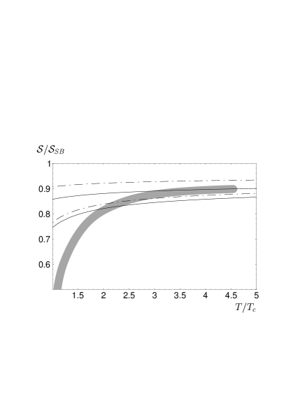
Figure 11: Comparison of results from approximately self-consistent thermodynamics based on the HTL propagator and a next-to-leading approximation (NLA) using the analogue of (147) for the asymptotic gluon mass correction (142) with lattice data from Boyd:1996bx . The gray band gives roughly the lattice data with their errors. The analytical results are given with two boundaries corresponding to a variation of the $\overline{\mbox{MS}}$ renormalization scale $\bar{\mu}$ from $\pi T$ to $4\pi T$

An optimistic conclusion one could draw from this is that the transition to gluonic and quark quasi-particles is able to absorb a large part of the strong elementary interaction into the spectral properties of the former, and that, at least in infrared-safe situations, these quasi-particles have comparatively weak residual interactions even in QCD at temperatures a few times above the transition temperature.

Let me recall that even in the infrared-unsafe case of NLO corrections to the Debye mass, the self-consistent NLO result (115) using a phenomenological magnetic mass gives the qualitatively correct result of a substantially increased electric mass, while underestimating the magnitude of the increase by a factor of 3 when compared to lattice simulations of chromoelectrostatic propagators.

7 Conclusions

Let us summarize the findings that are of specific interest to a perturbative formulation of non-Abelian gauge theories at finite temperature and/or density:

The leading-order results for self-energies and vertices in a high-temperature/density expansion, the so-called hard thermal (dense) loops, form a gauge-invariant and gauge-independent effective action, which is the basis for a systematic perturbative expansion in powers of $g$ (rather than $g^{2}$), as long as one does not run into the perturbative barrier formed by the completely non-perturbative self-interacting chromomagnetostatic modes.

Beyond leading order, gauge dependences appear in all Green functions of the fundamental fields. In particular the propagators which are expected to carry information on gluonic or fermionic quasi-particles depend on gauge-fixing parameters. The gauge dependence identities that we have discussed above imply, however, that under certain conditions the location of the singularities which define the dispersion laws of these quasi-particles are gauge-independent, though not e.g. residues or even the type of the singularities, which need not be simple poles.

Already at NLO, screening lengths and damping constants are logarithmically infrared sensitive to the nonperturbative magnetostatic sector, with the exception of zero 3-momentum. Infrared-safe quantities are also the real corrections to the dispersion laws, which in the case of longitudinal plasmons (and also of the plasmino branch of fermions) lead to a finite 3-momentum range, and, at its upper end, to space-like phase velocities. In the case of transverse gluonic quasiparticles and the normal branch of fermionic ones, the NLO corrections play an important role in self-consistent formulations of thermodynamics (the equation of state).

Particularly in QCD, one faces the problem that corrections to LO results are rather large for almost all values of the coupling of interest. However, we have seen indications that this poor convergence of thermal perturbation theory may be overcome in approximately self-consistent reformulations. Where those can be implemented, the picture of weakly interacting quasi-particles even in strong interactions seems to have some support from comparison with lattice data (where the latter are available), and may remain valid down to a few times the deconfinement phase transition temperature. This picture, being primarily set up in real Minkowski space, is complementary to lattice or dimensional reduction formulations, and allows (analytical) calculations from first principles also where lattice gauge theory calculations are not (yet) feasible. Its potentials, in particular when combined with results from other nonperturbative approaches, are, in my opinion, not yet fully explored.

References

- (1) A. Abada, O. Azi: Phys. Lett. B463, 117 (1999)
- (2) A. Abada, O. Azi, K. Benchallal: Phys. Lett. B425, 158 (1998)
- (3) L. F. Abbott: Nucl. Phys. B185, 189 (1981)
- (4) T. Altherr, E. Petitgirard, T. del Rio Gaztelurrutia: Phys. Rev. D47, 703 (1993)
- (5) J. O. Andersen, E. Braaten, M. Strickland: Phys. Rev. Lett. 83, 2139 (1999)
- (6) J. O. Andersen, E. Braaten, M. Strickland: Phys. Rev. D61, 014017 (2000)
- (7) J. O. Andersen, E. Braaten, M. Strickland: Phys. Rev. D61, 074016 (2000)
- (8) J. O. Andersen, E. Braaten, M. Strickland: Phys. Rev. D63, 105008 (2001)
- (9) P. Arnold, O. Espinosa: Phys. Rev. D47, 3546 (1993)
- (10) P. Arnold, L. G. Yaffe: Phys. Rev. D52, 7208 (1995)
- (11) P. Arnold, C.-X. Zhai: Phys. Rev. D50, 7603 (1994)
- (12) P. Arnold, C.-X. Zhai: Phys. Rev. D51, 1906 (1995)
- (13) P. Aurenche, F. Gelis, R. Kobes, E. Petitgirard: Phys. Rev. D54, 5274 (1996)
- (14) P. Aurenche, F. Gelis, R. Kobes, E. Petitgirard: Z. Phys. C75, 315 (1997)
- (15) R. Baier, O. K. Kalashnikov: Phys. Lett. B328, 450 (1994)
- (16) R. Baier, G. Kunstatter, D. Schiff: Nucl. Phys. B388, 287 (1992)
- (17) R. Baier, G. Kunstatter, D. Schiff: Phys. Rev. D45, 4381 (1992)
- (18) R. Baier, S. Peigné, D. Schiff: Z. Phys. C62, 337 (1994)
- (19) P. M. Bakshi, K. T. Mahanthappa: J. Math. Phys. 4, 1 (1963)
- (20) C. W. Bernard: Phys. Rev. D9, 3312 (1974)
- (21) J. P. Blaizot, E. Iancu: Phys. Rev. Lett. 70, 3376 (1993)
- (22) J. P. Blaizot, E. Iancu: Nucl. Phys. B417, 608 (1994)
- (23) J.-P. Blaizot, E. Iancu: Phys. Rev. Lett. 76, 3080 (1996)
- (24) J.-P. Blaizot, E. Iancu: Phys. Rev. D55, 973 (1997)
- (25) J.-P. Blaizot, E. Iancu: Phys. Rev. D56, 7877 (1997)
- (26) J.-P. Blaizot, E. Iancu: The quark-gluon plasma: Collective dynamics and hard thermal loops, hep-ph/0101103 (2001)
- (27) J.-P. Blaizot, E. Iancu, R. R. Parwani: Phys. Rev. D52, 2543 (1995)
- (28) J. P. Blaizot, E. Iancu, A. Rebhan: Phys. Rev. Lett. 83, 2906 (1999)
- (29) J. P. Blaizot, E. Iancu, A. Rebhan: Phys. Lett. B470, 181 (1999)
- (30) J. P. Blaizot, E. Iancu, A. Rebhan: Phys. Rev. D63, 065003 (2001)
- (31) N. N. Bogoliubov, D. V. Shirkov: Introduction to the theory of quantized fields (Interscience Publishers, New York, 1959)
- (32) G. Boyd, et al.: Nucl. Phys. B469, 419 (1996)
- (33) E. Braaten, A. Nieto: Phys. Rev. Lett. 73, 2402 (1994)
- (34) E. Braaten, A. Nieto: Phys. Rev. Lett. 74, 3530 (1995)
- (35) E. Braaten, A. Nieto: Phys. Rev. D53, 3421 (1996)
- (36) E. Braaten, R. D. Pisarski: Phys. Rev. D42, 2156 (1990)
- (37) E. Braaten, R. D. Pisarski: Nucl. Phys. B339, 310 (1990)
- (38) E. Braaten, R. D. Pisarski: Phys. Rev. Lett. 64, 1338 (1990)
- (39) E. Braaten, R. D. Pisarski: Nucl. Phys. B337, 569 (1990)
- (40) E. Braaten, R. D. Pisarski: Phys. Rev. D46, 1829 (1992)
- (41) E. Braaten, R. D. Pisarski: Phys. Rev. D45, 1827 (1992)
- (42) C. P. Burgess, A. L. Marini: Phys. Rev. D45, 17 (1992)
- (43) S. Chiku, T. Hatsuda: Phys. Rev. D58, 076001 (1998)
- (44) J. M. Cornwall, W.-S. Hou, J. E. King: Phys. Lett. B153, 173 (1985)
- (45) A. Cucchieri, F. Karsch, P. Petreczky: Phys. Lett. B497, 80 (2001)
- (46) A. Cucchieri, F. Karsch, P. Petreczky: Propagators and dimensional reduction of hot SU(2) gauge theory, hep-lat/0103009 (2001)
- (47) B. S. DeWitt: Phys. Rev. 162, 1195 (1967)
- (48) M. Dirks, A. Niegawa, K. Okano: Phys. Lett. B461, 131 (1999)
- (49) L. Dolan, R. Jackiw: Phys. Rev. D9, 3320 (1974)
- (50) I. T. Drummond, R. R. Horgan, P. V. Landshoff, A. Rebhan: Nucl. Phys. B524, 579 (1998)
- (51) I. T. Drummond, R. R. Horgan, P. V. Landshoff, A. Rebhan: Phys. Lett. B460, 197 (1999)
- (52) R. Efraty, V. P. Nair: Phys. Rev. Lett. 68, 2891 (1992)
- (53) R. Efraty, V. P. Nair: Phys. Rev. D47, 5601 (1993)
- (54) F. Flechsig: Nucl. Phys. B547, 239 (1999)
- (55) F. Flechsig, A. K. Rebhan: Nucl. Phys. B464, 279 (1996)
- (56) F. Flechsig, A. K. Rebhan, H. Schulz: Phys. Rev. D52, 2994 (1995)
- (57) F. Flechsig, H. Schulz: Phys. Lett. B349, 504 (1995)
- (58) E. S. Fradkin: Proc. Lebedev Inst. 29, 1 (1965)
- (59) J. Frenkel, J. C. Taylor: Nucl. Phys. B334, 199 (1990)
- (60) J. Frenkel, J. C. Taylor: Nucl. Phys. B374, 156 (1992)
- (61) T. Furusawa, K. Kikkawa: Phys. Lett. B128, 218 (1983)
- (62) F. Gelis: Phys. Lett. B455, 205 (1999)
- (63) M. Gell-Mann, K. A. Brueckner: Phys.Rev. 106, 364 (1957)
- (64) D. J. Gross, R. D. Pisarski, L. G. Yaffe: Rev. Mod. Phys. 53, 43 (1981)
- (65) T. H. Hansson, I. Zahed: Nucl. Phys. B292, 725 (1987)
- (66) H. Hata, T. Kugo: Phys. Rev. D21, 3333 (1980)
- (67) U. Heinz, K. Kajantie, T. Toimela: Ann. Phys. 176, 218 (1987)
- (68) U. M. Heller, F. Karsch, J. Rank: Phys. Rev. D57, 1438 (1998)
- (69) W. Israel: Physica 106A, 204 (1981)
- (70) K. A. James: Z. Phys. C48, 169 (1990)
- (71) K. A. James, P. V. Landshoff: Phys. Lett. B251, 167 (1990)
- (72) K. Kajantie, J. Kapusta: Phys. Lett. B110, 299 (1982)
- (73) K. Kajantie, J. Kapusta: Ann. Phys. 160, 477 (1985)
- (74) K. Kajantie, et al.: Phys. Rev. Lett. 79, 3130 (1997)
- (75) O. K. Kalashnikov, V. V. Klimov: Sov. J. Nucl. Phys. 31, 699 (1980)
- (76) J. I. Kapusta: Finite-temperature field theory (Cambridge University Press, Cambridge, UK, 1989)
- (77) F. Karsch, A. Patkós, P. Petreczky: Phys. Lett. B401, 69 (1997)
- (78) L. V. Keldysh: Zh. Eksp. Teor. Fiz. 47, 1515 (1964)
- (79) P. F. Kelly, Q. Liu, C. Lucchesi, C. Manuel: Phys. Rev. D50, 4209 (1994)
- (80) V. V. Klimov: Sov. J. Nucl. Phys. 33, 934 (1981)
- (81) R. Kobes, G. Kunstatter, K. Mak: Phys. Rev. D45, 4632 (1992)
- (82) R. Kobes, G. Kunstatter, A. Rebhan: Phys. Rev. Lett. 64, 2992 (1990)
- (83) R. Kobes, G. Kunstatter, A. Rebhan: Nucl. Phys. B355, 1 (1991)
- (84) U. Kraemmer, M. Kreuzer, A. Rebhan: Ann. Phys. 201, 223 (1990)
- (85) U. Kraemmer, A. K. Rebhan, H. Schulz: Ann. Phys. 238, 286 (1995)
- (86) T. Kugo, I. Ojima: Phys. Lett. B73, 459 (1978)
- (87) T. Kugo, I. Ojima: Prog. Theor. Phys. 61, 644 (1979)
- (88) M. Laine, O. Philipsen: Nucl. Phys. B523, 267 (1998)
- (89) M. Laine, O. Philipsen: Phys. Lett. B459, 259 (1999)
- (90) P. V. Landshoff, A. Rebhan: Nucl. Phys. B383, 607 (1992)
- (91) P. V. Landshoff, A. Rebhan: Nucl. Phys. B410, 23 (1993)
- (92) N. P. Landsman, C. G. van Weert: Phys. Rept. 145, 141 (1987)
- (93) M. Le Bellac: Thermal Field Theory (Cambridge University Press, Cambridge, UK, 1996)
- (94) V. V. Lebedev, A. V. Smilga: Ann. Phys. 202, 229 (1990)
- (95) V. V. Lebedev, A. V. Smilga: Phys. Lett. B253, 231 (1991)
- (96) A. D. Linde: Phys. Lett. B96, 289 (1980)
- (97) T. Matsubara: Prog. Theor. Phys. 14, 351 (1955)
- (98) H. Matsumoto, Y. Nakano, H. Umezawa: Phys. Rev. D28, 1931 (1983)
- (99) H. Matsumoto, Y. Nakano, H. Umezawa: J. Math. Phys. 25, 3076 (1984)
- (100) L. D. McLerran, B. Svetitsky: Phys. Rev. D24, 450 (1981)
- (101) S. Nadkarni: Phys. Rev. D33, 3738 (1986)
- (102) S. Nadkarni: Phys. Rev. Lett. 61, 396 (1988)
- (103) V. P. Nair: Phys. Rev. D48, 3432 (1993)
- (104) A. Niegawa: Phys. Rev. D40, 1199 (1989)
- (105) S. Peigné, E. Pilon, D. Schiff: Z. Phys. C60, 455 (1993)
- (106) S. Peigné, S. M. H. Wong: Phys. Lett. B346, 322 (1995)
- (107) R. D. Pisarski: Nucl. Phys. A498, 423C (1989)
- (108) R. D. Pisarski: Phys. Rev. Lett. 63, 1129 (1989)
- (109) R. D. Pisarski: Phys. Rev. D47, 5589 (1993)
- (110) A. M. Polyakov: Phys. Lett. B72, 477 (1978)
- (111) K. Rajagopal, E. Shuster: Phys. Rev. D62, 085007 (2000)
- (112) A. Rebhan: Nucl. Phys. B288, 832 (1987)
- (113) A. Rebhan: Phys. Rev. D46, 482 (1992)
- (114) A. Rebhan: Phys. Rev. D46, 4779 (1992)
- (115) A. K. Rebhan: Phys. Rev. D48, 3967 (1993)
- (116) A. K. Rebhan: Nucl. Phys. B430, 319 (1994)
- (117) H. Schulz: Nucl. Phys. B413, 353 (1994)
- (118) J. Schwinger: J. Math. Phys. 2, 407 (1961)
- (119) V. P. Silin, V. N. Ursov: Sov. Phys. - Lebedev Inst. Rep. 5, 43 (1988)
- (120) J. C. Taylor, S. M. H. Wong: Nucl. Phys. B346, 115 (1990)
- (121) T. Toimela: Z. Phys. C27, 289 (1985)
- (122) V. N. Tsytovich: Sov. Phys. (JETP) 13, 1249 (1961)
- (123) G. A. Vilkovisky: Nucl. Phys. B234, 125 (1984)
- (124) H. A. Weldon: Phys. Rev. D26, 1394 (1982)
- (125) H. A. Weldon: Phys. Rev. D40, 2410 (1989)
- (126) C.-X. Zhai, B. Kastening: Phys. Rev. D52, 7232 (1995)