ILL-(TH)-01-02
hep-ph/0105042
The Standard Model on a D-brane

We present a consistent string theory model which reproduces the Standard Model, consisting of a $D3$-brane at a simple orbifold singularity. We study some simple features of the phenomenology of the model. We find that the scale of stringy physics must be in the multi-TeV range. There are natural hierarchies in the fermion spectrum and there are several possible experimental signatures of the model.

1 Introduction

A common thread in recent new proposals for physics beyond the Standard Model is the realization of the gauge theory on a brane. In string theory terms, this is presumably a D-brane. In this note, we will study a remarkably conservative realization of the Standard Model in a fully consistent string background. The local geometry is (a deformation of) the orbifold ${\mathbb{R}}^{4}\times{\mathbb{C}}^{3}/\Gamma$ with the brane extended along the ${\mathbb{R}}^{4}$. $\Gamma$ is a particular non-Abelian discrete subgroup of $SU(3)$.

There are several interesting features present. First, there is a natural hierarchy between the masses of leptons and quarks, because superpotential lepton Yukawa couplings are forbidden by continuous gauge symmetries. We find, however, that it is possible to achieve a realistic lepton mass spectrum through Kähler potential terms after supersymmetry breaking. Assuming that these nonrenormalizable terms are generated (at tree level) at the string scale, the string scale must be in the multi-TeV range. We will not consider the global geometry off the D-brane in detail here, but it should be noted that this geometry must give rise to the TeV range string scale as well as supersymmetry breaking. We will parametrize this breaking through effective spurion couplings in the Kähler potential. Secondly, there are two additional gauged $U(1)$ symmetries that are broken only at the weak scale. The phenomenology of these symmetries deserves further study, but their presence does not seem to be in conflict with experimental results.

2 The Orbifold Model

Consider a $D3$-brane at an isolated orbifold point in ${\mathbb{C}}^{3}/\Gamma$, where $\Gamma=\Delta_{27}$, one of the non-Abelian discrete subgroups of $SU(3)$. As such, the resulting gauge theory has $N=1$ supersymmetry. The group is one of the $\Delta_{3n^{2}}$ series, defined by the short exact sequence

$$0\rightarrow{\mathbb{Z}}_{n}\times{\mathbb{Z}}_{n}\rightarrow\Delta_{3n^{2}}\rightarrow{\mathbb{Z}}_{3}\rightarrow 0.$$ (1)

They are generated by three elements $e_{1},e_{2},e_{3}$ whose action on ${\mathbb{C}}^{3}$ is given by

$$e_{1}: (z_{1},z_{2},z_{3})\rightarrow(\omega_{n}z_{1},\omega_{n}^{-1}z_{2},z_{3}),$$

$$e_{2}: (z_{1},z_{2},z_{3})\rightarrow(z_{1},\omega_{n}z_{2},\omega_{n}^{-1}z_{3}),$$ (2)

$$e_{3}: (z_{1},z_{2},z_{3})\rightarrow(z_{3},z_{1},z_{2}),$$

where $\omega_{n}$ is an $n$-th root of unity. The quivers [1] of the $\Delta_{3n^{2}}$ groups are discussed in Refs. [2, 3, 4, 5, 6]. For the case $n=3$ that we are interested in, the quiver is as shown in Figure 1.

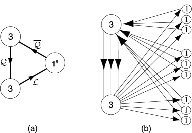
Figure 1: Two views of the quiver diagram of the $\Delta_{27}$ singularity.

The gauge group is $\left(U(3)_{+}\times U(3)_{-}\times U(1)^{9}\right)/U(1)$, and the matter fields transform in the representations ${\cal Q}_{i}=({\bf 3}_{+},\overline{{\bf 3}}_{-},0)$, ${\cal L}_{a}=({\bf 1}_{0},{\bf 3}_{+},-_{a})$, and $\overline{{\cal Q}}_{a}=(\overline{{\bf 3}}_{-},{\bf 1}_{0},+_{a})$, where the index $a$ runs over the nine $U(1)$’s and $i=1,\ldots,3$. The plus and minus subscripts denote the $U(1)$ charge under the decomposition $U(3)\sim SU(3)\times U(1)$. Each of the fields ${\cal L}_{a}$ and $\overline{{\cal Q}}_{a}$ are charged under only one of the nine $U(1)$’s. We will identify the $SU(3)$ subgroup of $U(3)_{+}$ with the color group and $SU(2)_{W}$ is embedded in the $U(3)_{-}$ group. The orbifold theory comes with a renormalizable superpotential generated at string tree-level of the form

$$W_{0}=\sum_{ia}\lambda_{ia}{\cal Q}_{i}{\cal L}_{a}\overline{{\cal Q}}_{a},$$ (3)

where the $\lambda_{ia}$ are couplings of order one at the string scale. We will study this superpotential in detail in what follows.

The orbifold has a number of moduli that we will exploit. There are two issues to be addressed: first, at the orbifold point (i.e. all moduli vevs are zero), the gauge couplings of the various group factors are related to one another. However, there are closed string moduli whose vevs shift the values of the various gauge couplings, and so allowing for this, we may set the couplings as needed. A second issue is that we wish to break some of the gauge symmetry: the $U(3)_{W}$ should be broken to $SU(2)_{W}$, and at least some of the $U(1)$’s removed. For the former, there are moduli corresponding to Fayet-Iliopoulos (FI) terms $\int d^{4}\theta\,r_{a}V_{a}$ for the $U(1)$’s. The resulting $D$-term equations are

$$r_{a}-\langle{{\cal L}_{a}^{\dagger}{\cal L}_{a}}\rangle+\langle{\overline{{\cal Q}}_{a}^{\dagger}\overline{{\cal Q}}_{a}}\rangle=0,$$ (4)

and thus there are vacua where $\langle{{\cal L}_{a}}\rangle\neq 0$. We will suppose that six of the nine vevs are non-zero. For clarity however, we will consider only three such vevs. This is sufficient to display the structure of the non-Abelian symmetry breaking pattern, and the inclusion of additional vevs will be accounted for later. Thus for now, we will suppose that three of the FI terms are non-zero and positive, $r_{1,2,3}>0$. Then the solutions $\langle{{\cal L}_{1,2,3}}\rangle\neq 0$ may be chosen to break $U(3)_{W}\times U(1)^{3}$ to $SU(2)_{W}\times U(1)_{0}$; $U(3)_{c}$ and the remaining six $U(1)$’s are unbroken by these three vevs. Note that under this breaking pattern, we may write (for $i=1,2,3$)

$$\begin{array}[]{ccclc}{\cal Q}_{i}&\to&Q_{i}&,&q_{i}\\ {\cal L}_{1,i}&\to&L_{i}&,&g_{i}\\ {\cal L}_{2,i}&\to&H_{i}&,&\overline{e}_{i}\\ {\cal L}_{3,i}&\to&\overline{H}_{i}&,&\overline{\nu}_{i}\end{array}$$ (5)

and we now make the identification

$$\overline{{\cal Q}}_{1,i}\to\overline{q}_{i},\ \ \ \ \overline{{\cal Q}}_{2,i}\to\overline{u}_{i},\ \ \ \ \overline{{\cal Q}}_{3,i}\to\overline{d}_{i}.$$ (6)

The notation is that of the Standard Model, apart from the superfields $q,\overline{q},g$. The fields $g_{i}$ are those that have vacuum expectation values. The $q_{j},\overline{q}_{j}$ have a mass of order $\lambda_{ij}\langle{g}\rangle_{i}$ and may be integrated out. Thus, we are left with the superfields of the three generation Standard Model, including neutrino singlets, with six Higgs doublet superfields. With this notation, the superpotential may be written

$$W=\sum_{ij}\left\{a_{ij}\left[Q_{i}H_{j}+q_{i}\overline{e}_{j}\right]\overline{u}_{j}+b_{ij}\left[Q_{i}\overline{H}_{j}+q_{i}\overline{\nu}_{j}\right]\overline{d}_{j}+c_{ij}\left[Q_{i}L_{j}+q_{i}{g_{j}}\right]\overline{q}_{j}\right\},$$ (7)

and in the broken phase becomes (unitary gauge)

$$W_{\rm eff}=\sum_{ij}\left\{a_{ij}H_{j}Q_{i}\overline{u}_{j}+b_{ij}\overline{H}_{j}Q_{i}\overline{d}_{j}-\tilde{a}_{ijk}Q_{i}\overline{u}_{k}L_{j}\overline{e}_{k}-\tilde{b}_{ijk}Q_{i}\overline{d}_{k}L_{j}\overline{\nu}_{k}\right\}.$$ (8)

We note that quark Yukawa couplings are present at tree level, but lepton Yukawas are not. In addition, there are no $\mu$ terms, as all quadratic terms are forbidden by gauge symmetries.

Now, there are additional vevs that could be turned on without further breaking the Standard Model gauge group. In the notation presented here, these are the three sneutrinos $\overline{\nu}_{j}$. These vevs have several virtues, primarily in that they break additional $U(1)$ symmetries, but also that they are necessary, as we will see later, for realistic fermion masses. The one thing that should be noted here is that if $\langle{\overline{\nu}}\rangle\neq 0$, then there are some field redefinitions that need to be done (e.g., in eq. (8) it can be seen that $L$ mixes with $\overline{H}$; there is also mixing with massive gauginos because of $SU(3)_{-}$ breaking).

3 Anomalies and the Fate of the $U(1)$’s

Let us discuss the unbroken gauge group in some detail. At the orbifold point there are ten $U(1)$’s. We find that there are the following non-zero gauge anomalies

$$U(3)_{\pm}U(3)_{\pm}U(1)_{\mp}: \mp 3\sqrt{3},$$

$$U(3)_{\pm}U(3)_{\pm}U(1)_{a}: \pm\sqrt{3},$$ (9)

$$U(1)_{a}U(1)_{a}U(1)_{\pm}: \mp 3\sqrt{3}.$$

There are no gravitational or mixed anomalies. The generalized Green-Schwarz mechanism (involving the NSNS B-field as well as twisted moduli)[8, 9, 1, 10] will serve to cancel these anomalies and consequently will break some of the $U(1)$’s. The generators of the broken $U(1)$’s are $3Y_{\pm}\mp\sum_{a}Y_{a}$. Since the $U(1)$ generated by $Y_{+}+Y_{-}+\sum_{a}Y_{a}$ decouples, we can conclude that all surviving generators are orthogonal to $Y_{\pm}$ as well as $\sum_{a}Y_{a}$. Note also that since baryon number may be identified with $U(1)_{+}$, there are no perturbative baryon number violating processes such as proton decay, as the global symmetry survives the Green-Schwarz mechanism; see also [11] where the same mechanism was realized in a different model.

Now, if we consider the $g$ and $\overline{\nu}$ vevs, there is an unbroken $U(1)$ generator which we call $Q_{0}$; this is a linear combination of $Q_{8-}$ (the diagonal generator of $SU(3)_{-}$) and six of the nine $U(1)$’s:

$$Q_{0}=\sqrt{6}Q_{8-}-2\sum_{j}(Q_{1,j}+Q_{3,j}).$$ (10)

This can be mixed with a linear combination of the $Q_{2,j}$’s as long as we take a non-anomalous combination. Thus, we identify the hypercharge generator

$$Y=-\left[Q_{0}+4\sum_{i=1}^{3}\left(Q_{2,i}\right)\right]/6.$$ (11)

The $U(1)$ charges in the low energy theory are tabulated below.

$$\begin{array}[]{|c||r|r|r|r|r|}\hline\cr&U(1)_{0}&U(1)_{1}&U(1)_{2}&U(1)_{3}\\ \hline\cr\hline\cr Q&-1&0&0&0\\ \hline\cr\overline{u}&0&0&1&0\\ \hline\cr\overline{d}&-2&0&0&1\\ \hline\cr L&3&-1&0&0\\ \hline\cr\overline{e}&-2&0&-1&0\\ \hline\cr\overline{\nu}&0&0&0&-1\\ \hline\cr H&1&0&-1&0\\ \hline\cr\overline{H}&3&0&0&-1\\ \hline\cr g&0&-1&0&0\\ \hline\cr q&2&0&0&0\\ \hline\cr\overline{q}&-2&1&0&0\\ \hline\cr\end{array}$$ (12)

There are two other unbroken non-anomalous $U(1)$’s present other than hypercharge. We can take these to be $Q_{2,1}-Q_{2,3}$ and $Q_{2,2}-Q_{2,3}$. Under these two symmetries, only $\overline{u}_{j},\overline{e}_{j}$ and $H_{j}$ are charged, as can be seen by looking at the table. We will comment later on the possibly interesting phenomenology associated with these extra $U(1)$ symmetries, which are broken at the weak scale.

4 Mass Spectrum, Couplings and Supersymmetry
Breaking

From the superpotential, eq. (8), we see that the quark sector has standard Yukawa couplings giving rise to supersymmetric mass terms

$$(m_{u})_{ij}=a_{ij}\langle{H_{j}}\rangle,\ \ \ \ \ \ (m_{d})_{ij}=b_{ij}\langle{\overline{H}_{j}}\rangle.$$ (13)

There are no Yukawa couplings present for the leptons, a consequence of the gauged $U(1)$ symmetries of the orbifold. We regard this as a strong feature of the model: the lepton masses are hierarchically suppressed compared to quark masses. We need to demonstrate of course that lepton masses can be generated. Because of the symmetries, the lepton masses must be generated through Kähler potential terms, as follows. There will be terms of the general form

$$K\supset\frac{1}{M^{2}}\alpha_{ab}({\cal L}_{a}^{\dagger}{\cal L}_{b})({\cal L}^{\dagger}_{b}{\cal L}_{a})+\frac{1}{M^{2}}\alpha^{\prime}_{ab}({\cal L}_{a}^{\dagger}{\cal L}_{a})({\cal L}^{\dagger}_{b}{\cal L}_{b}).$$ (14)

In particular, we will find terms

$$\alpha_{ij}g_{i}^{\dagger}\overline{e}_{j}H_{j}^{\dagger}L_{i}+\beta_{ij}g_{i}^{\dagger}\overline{\nu}_{j}\overline{H}^{\dagger}_{j}L_{i}$$ (15)

which give rise to charged lepton fermion masses of the form

$$(m_{L})_{ij}\sim\alpha_{ij}\frac{F_{g_{i}}^{*}}{M^{2}}\langle{H^{*}_{j}}\rangle$$ (16)

and neutrino Dirac masses

$$(m_{D})_{ij}\sim\beta_{ij}\frac{F_{g_{i}}^{*}}{M^{2}}\langle{\overline{H}^{*}_{j}}\rangle.$$ (17)

From these equations it is clear that the generation of lepton Yukawas are intimately tied with the supersymmetry breaking scale and each of them is hierarchically suppressed.

Supersymmetry may be broken in a variety of ways in brane models. We will take an agnostic approach, and simply write the effects of supersymmetry breaking in terms of spurion couplings. For example, we will take the Kähler potential to contain terms

$$K=\ldots+\frac{1}{M}S\sum\phi_{i}^{\dagger}\phi_{i}+\frac{1}{M^{2}}\Psi^{\dagger}\Psi\phi_{i}^{\dagger}\phi_{i}+\ldots,$$ (18)

where the $\phi_{i}$ are any of the open string modes. The spurions $S$ and $\Psi$ may very well be closed string modes, which we would expect to couple universally to the open string modes. We will make the assumption that $\langle{\Psi}\rangle\sim\theta^{2}F\sim\langle{S}\rangle$, so that $m_{susy}\sim F/M$. The scale $M$ is some high energy scale, which we identify with the string scale. Note that with the Kähler potential given, we find that open string fields may have $F$-terms of the form

$$F_{i}\sim\frac{F\langle{\phi_{i}}\rangle}{M}\sim m_{susy}\langle{\phi_{i}}\rangle.$$ (19)

Under these conditions the lepton masses are suppressed by a factor $m_{susy}\langle{g}\rangle/M^{2}$ according to (19). For this reason $M$ cannot be too far above the supersymmetry breaking scale $m_{susy}$. A possible scenario is where $M\sim$ 10 TeV, $\langle{g}\rangle\sim\langle{\overline{\nu}}\rangle\sim$ 1 TeV, $m_{susy}\sim$ 3 TeV. Of course, in order to obtain a realistic spectrum, the neutrino masses must be suppressed compared to the charged leptons. By the same mechanism, there are also neutrino Majorana masses of the form

$$\gamma_{ij}\frac{F_{\overline{\nu}_{i}}^{*}\langle{\overline{\nu}^{*}_{j}}\rangle}{M^{2}}$$ (20)

Comparing to the Dirac masses, we see that these are larger, and thus a seesaw can occur. Roughly, we have

$$\frac{m_{\nu}}{m_{L}}\sim\frac{\beta^{2}}{\alpha\gamma}\frac{\langle{H}\rangle\langle{g}\rangle}{\langle{\overline{\nu}}\rangle^{2}}\left(\frac{\langle{\overline{H}}\rangle}{\langle{H}\rangle}\right)^{2}.$$ (21)

The simplest way that the mass hierarchy between up and down type quarks may be obtained is to take $\langle{\overline{H}}\rangle<\langle{H}\rangle$ (large $\tan\beta$) and we see that the light neutrino masses are suppressed by two powers of $\tan\beta$. This is probably not sufficient, but note that there are several other mechanisms available here to suppress neutrino masses. First, there may be small differences in coupling constants, and possibly a difference between $\langle{g}\rangle$ and $\langle{\overline{\nu}}\rangle$. As well, since there are six Higgs doublets, there may be a hierarchy of vevs which could further suppress low generation neutrino masses. We conclude that there is ample parameter space to obtain a realistic lepton mass and mixing spectrum.

All superpartners receive diagonal supersymmetry breaking masses of order $m_{susy}$, since the scalar masses coming from (18) are universal. There are also off-diagonal masses which would come about through Kähler potential terms of the form

$$K\supset\frac{1}{M^{2}}\alpha_{ij,a}({\cal Q}^{\dagger}_{i}{\cal Q}_{j})({\cal L}^{\dagger}_{a}{\cal L}_{a})+\beta_{ab}(\overline{{\cal Q}}^{\dagger}_{a}\overline{{\cal Q}}_{a})({\cal L}^{\dagger}_{b}{\cal L}_{b})+\gamma_{ab}(\overline{{\cal Q}}^{\dagger}_{a}\overline{{\cal Q}}_{b})({\cal L}^{\dagger}_{a}{\cal L}_{b}).$$ (22)

Thus, there are off-diagonal scalar masses, for example

$$(m_{Q}^{2})_{ij}\sim\frac{\alpha_{ij,a}|F_{a}|^{2}}{M^{2}}\sim\frac{\alpha_{ij,a}|\langle{g_{a}}\rangle|^{2}}{M^{2}}m_{susy}^{2}.$$ (23)

As a result, there is some suppression here of flavor changing neutral currents. We have not done a complete analysis, but it appears that they may be at or below experimental limits.

Notice also that each of the right-handed quarks couples to a different Higgs multiplet. Hence one can keep all couplings of the same order of magnitude and produce the mass hierarchy between generations by having a hierarchy of vevs. Also, the CKM matrix may turn out to be nearly diagonal because of approximate discrete symmetries that can appear near the orbifold point. This same discrete symmetry might account for the hierarchy between the generations.

5 Discussion

We have presented here a consistent string model giving rise in the low energy limit to a gauge theory which closely resembles the Standard Model. The phenomenology of the model is rich. Lepton masses are hierarchically suppressed compared to quark masses, and it appears, at least at the level of analysis done here, that a realistic spectrum is possible. An important aspect of the phenomenology is that we must arrange that the string scale is low, thus the Planck mass in four dimensions can be attributed to large extra dimensions [12, 13] or a Randall-Sundrum type model [14]. A possible scenario is where $M\sim$ 10 TeV, $\langle{g}\rangle\sim\langle{\overline{\nu}}\rangle\sim$ 1 TeV, $m_{susy}\sim$ 3 TeV. The model possesses six Higgs fields, a pair for each generation, and thus there is some flexibility in the fermion spectrum. We have not dealt with the details of the Higgs spectrum; several of these may be heavy because of supersymmetry breaking effects, there is mixing with sleptons and $SU(3)_{-}$ breaking removes one linear combination from the low energy spectrum. The spectrum of neutrino masses is also an interesting feature—it would be interesting to explore this further in light of present experiments. There are several additional aspects of the phenomenology that deserve more careful consideration. These include flavor changing neutral currents, and the presence of relatively light extra gauge bosons. These symmetries are broken at the weak scale by Higgs vevs, but it should be noted that these gauge bosons do not have weak-style couplings, and hence the experimental constraints are not immediately apparent.

Acknowledgments: Discussions with S. Willenbrock are gratefully acknowledged. Supported in part by U.S. Department of Energy, grant DE-FG02-91ER40677. VJ is supported by a GAANN fellowship from the U.S. Department of Education, grant 1533616.

References

• [1] M.Β R. Douglas and G.Β Moore, β€œD-branes, Quivers, and ALE Instantons,” hep-th/9603167.
• [2] B.Β R. Greene, C.Β I. Lazaroiu, and M.Β Raugas, β€œD-branes on nonabelian threefold quotient singularities,” Nucl. Phys. B553 (1999) 711–749, hep-th/9811201.
• [3] T.Β Muto, β€œD-branes on three-dimensional nonabelian orbifolds,” JHEP 02 (1999) 008, hep-th/9811258.
• [4] T.Β Muto, β€œBrane configurations for three-dimensional nonabelian orbifolds,” hep-th/9905230.
• [5] A.Β Hanany and Y.-H. He, β€œNon-Abelian finite gauge theories,” JHEP 02 (1999) 013, hep-th/9811183.
• [6] D.Β Berenstein, V.Β Jejjala, and R.Β G. Leigh, β€œD-branes on singularities: New quivers from old,” hep-th/0012050.
• [7] G.Β Aldazabal, L.Β E. Ibanez, F.Β Quevedo, and A.Β M. Uranga, β€œD-branes at singularities: A bottom-up approach to the string embedding of the standard model,” JHEP 08 (2000) 002, hep-th/0005067.
• [8] M.Β B. Green and J.Β H. Schwarz, β€œAnomaly Cancellation in Supersymmetric D=10 Gauge Theory and Superstring Theory,” Phys. Lett. B149 (1984) 117–122.M.Β B. Green and J.Β H. Schwarz, β€œThe Hexagon Gauge Anomaly in Type I Superstring Theory,” Nucl. Phys. B255 (1985) 93–114. M.Β B. Green, J.Β H. Schwarz, and P.Β C. West, β€œAnomaly Free Chiral Theories in Six Dimensions,” Nucl. Phys. B254 (1985) 327–348.
• [9] M.Β B. Green, J.Β H. Schwarz, and E.Β Witten, β€œSuperstring Theory. Vol. 2: Loop Amplitudes, Anomalies and Phenomenology,”. Cambridge, Uk: Univ. Pr. (1987) 596 P. (Cambridge Monographs On Mathematical Physics).
• [10] M.Β Berkooz, R.Β G. Leigh, J.Β Polchinski, J.Β H. Schwarz, N.Β Seiberg, and E.Β Witten, β€œAnomalies, Dualities, and Topology of D=6 N=1 Superstring Vacua,” Nucl. Phys. B475 (1996) 115–148, hep-th/9605184.
• [11] I.Β Antoniadis, E.Β Kiritsis, and T.Β N. Tomaras, β€œA D-brane alternative to unification,” Phys. Lett. B486 (2000) 186–193, hep-ph/0004214.
• [12] N.Β Arkani-Hamed, S.Β Dimopoulos, and G.Β Dvali, β€œThe hierarchy problem and new dimensions at a millimeter,” Phys. Lett. B429 (1998) 263–272, hep-ph/9803315.
• [13] I.Β Antoniadis, N.Β Arkani-Hamed, S.Β Dimopoulos, and G.Β Dvali, β€œNew dimensions at a millimeter to a Fermi and superstrings at a TeV,” Phys. Lett. B436 (1998) 257–263, hep-ph/9804398.
• [14] L.Β Randall and R.Β Sundrum, β€œAn alternative to compactification,” Phys. Rev. Lett. 83 (1999) 4690–4693, hep-th/9906064.