Abstract

We resum Sudakov threshold enhancements in heavy quark hadroproduction for single-heavy quark inclusive and pair-inclusive kinematics. We expand these resummed results and derive analytical finite-order cross sections through next-to-next-to-leading order. This involves the construction of next-to-leading order matching conditions in color space. For the scale dependent terms we derive exact results using renormalization group methods. We study the effects of scale variations, scheme and kinematics choice on the partonic and hadronic cross sections, and provide estimates for top and bottom quark production cross sections.

1 Introduction

Long- and short-distance dynamics in inclusive hadronic hard-scattering cross sections are factorized in Quantum Chromodynamics (QCD) into universal, non-perturbative parton distribution functions and fragmentation functions, and perturbatively calculable hard scattering functions. Remnants of long-distance dynamics in a hard scattering function can, however, become large in regions of phase space near partonic threshold and dominate higher order corrections. Such Sudakov corrections assume the form of distributions that are singular at partonic threshold. Threshold resummation organizes these double-logarithmic corrections to all orders, thereby extending the predictive power of QCD to these phase space regions.

Early on [1, 2], the organization of such corrections to arbitrary logarithmic accuracy was achieved for the Drell-Yan cross section. An equivalent level of understanding for general QCD processes with more complex color structures at the Born level has been achieved more recently [3, 4, 5, 6, 7, 8]. The resummation of Sudakov corrections in such processes to next-to-leading logarithmic (NLL) accuracy requires understanding how these structures mix under soft gluon radiation. Many NLL-resummed cross sections have been calculated: heavy quark hadro- [4, 5, 8, 9, 10, 11, 12] and electroproduction [13, 14], dijet production [6, 7], single-jet production [15], Higgs production [16], prompt photon production [12, 17, 18, 19, 20] and hadroproduction of electroweak bosons [21]. For a recent review see Ref. [22]. The formalism of Refs. [3, 4, 5, 6, 7] and the one of Ref. [8] both allow arbitrary logarithmic accuracy. Processes involving Born-level two-particle scattering may be described in either single-particle inclusive or pair-inclusive kinematics. NLL resummation was initially performed in pair-inclusive kinematics [4, 5, 6, 7] and later extended to single-particle kinematics [12, 17].

Resummed cross sections constitute an approximate sum of the complete perturbative expansion if, at each order, the Sudakov corrections dominate. The numerical evaluation of resummed cross sections requires a prescription to handle infrared renormalon singularities. Resummed cross sections may also be expanded to provide estimates of finite higher order corrections which do not suffer from renormalon problems. In this paper we shall employ the resummed cross sections in the latter fashion: as generating functionals of approximate perturbation theory.

Resummed results for heavy quark production at leading logarithmic accuracy have been presented some time ago [24, 25, 26, 27, 28, 29]. In our paper we expand the NLL resummed cross sections presented in Refs. [4, 5, 12] and derive complete analytic expressions through next-to-next-to-leading order (NNLO) for double-differential heavy quark cross sections in two different kinematics: heavy quark pair-inclusive and single-heavy quark inclusive. To achieve next-to-next-to-leading logarithmic (NNLL) accuracy we include color-coherence effects and contributions due to soft radiation from one-loop virtual graphs via matching conditions.

Our paper is organized as follows. In section 2 we discuss both types of kinematics and their singular functions. Section 3 describes the construction of the resummed cross sections. In section 4 we expand the resummed cross section to NLO and NNLO and present analytical NNLL double-differential cross sections at each order, with both types of kinematics, in the gluon-gluon ($gg$) and quark-antiquark ($q\overline{q}$) channels. We numerically study the inclusive partonic and hadronic cross sections in sections 5 and 6 respectively. Our conclusions are presented in section 7. Appendix A contains the NLO matching terms for pair-inclusive kinematics. In appendix B we collect all our explicit expressions for the NLO and NNLO differential cross sections.

A companion study [30], also addressing third and fourth order corrections, contributions from subleading logarithms, and some differential distributions, already featuring some of the second order results for inclusive cross sections derived in this paper, was recently presented by one of us.

2 Kinematics and cross sections

The kinematics of inclusive heavy quark hadroproduction depend on which final state momenta are reconstructed. In threshold resummation this kinematics choice manifests itself at next-to-leading logarithmic level [12]. We discuss two types of near-elastic kinematics in heavy quark hadroproduction, one-particle inclusive (1PI) and pair-invariant mass (PIM) kinematics.

2.1 One-particle inclusive (1PI) kinematics

Heavy quark hadroproduction in 1PI kinematics is defined by

$$h_{1}(P_{1})+\,h_{2}(P_{2}) \longrightarrow {\rm{Q}}(p_{1})+\,X[{\overline{\rm{Q}}}](p_{X})\,,$$ (1)

where $h_{1}$ and $h_{2}$ are hadrons, $X[\overline{\rm{Q}}]$ denotes any allowed hadronic final state containing at least the heavy antiquark, and ${\rm{Q}}(p_{1})$ is the identified heavy quark with mass $m$. The hadronic invariants in this reaction are

$$S=(P_{1}+P_{2})^{2}\quad,\quad T_{1}=(P_{2}-p_{1})^{2}-m^{2}\quad,\quad U_{1}=(P_{1}-p_{1})^{2}-m^{2}\,,$$ (2)

and

$$S_{4}=S+T_{1}+U_{1}\,,$$ (3)

where $S_{4}$ is a measure of the inelasticity of the hadronic reaction (1). Near threshold, reaction (1) is dominated by the partonic subprocesses

$$q(k_{1})+\,{\overline{q}}(k_{2}) \longrightarrow {\rm{Q}}(p_{1})+\,X^{\prime}[{\overline{\rm{Q}}}](p_{2}^{\prime})\,,$$ (4)

$$g(k_{1})+\,g(k_{2}) \longrightarrow {\rm{Q}}(p_{1})+\,X^{\prime}[{\overline{\rm{Q}}}](p_{2}^{\prime})\,.$$ (5)

If $X^{\prime}[{\overline{\rm{Q}}}](p_{2}^{\prime})={\overline{\rm{Q}}}(\bar{p}_{2})$, the reaction is at partonic threshold and the heavy antiquark has momentum $\bar{p}_{2}$. Note that threshold production does not mean that the heavy quarks are produced at rest. The $qg$ and $\overline{q}g$ channels contribute at one order higher in $\alpha_{s}$ than the reactions (4) and (5). The partonic invariants corresponding to (2) are

$$s\,=\,(k_{1}+k_{2})^{2}\,,\hskip 28.45274ptt_{1}\,=\,(k_{2}-p_{1})^{2}-m^{2}\,,\hskip 28.45274ptu_{1}\,=\,(k_{1}-p_{1})^{2}-m^{2}\,.$$ (6)

The invariant $s_{4}=(p^{\prime}_{2})^{2}-m^{2}$ which measures the inelasticity of the partonic reactions (4) and (5) is related to the other partonic invariants by

$$s_{4} = s+t_{1}+u_{1}\,.$$ (7)

The inclusive partonic cross section may be calculated from

$$\sigma_{ij}(s,m^{2}) = \int\limits_{s(1-\beta)/2}^{s(1+\beta)/2}\,d(-t_{1})\int\limits_{0}^{s_{4}^{\rm max}}\,ds_{4}\,\,\,\frac{d^{2}\sigma_{ij}(s,t_{1},s_{4})}{dt_{1}\,ds_{4}}\,$$ (8)

where $\beta=\sqrt{1-4m^{2}/s}$ and

$$s_{4}^{\rm max} = s+t_{1}+\frac{sm^{2}}{t_{1}}\,.$$ (9)

The recoil momentum $p_{2}^{\prime}$ may be split into the momentum at threshold, $\bar{p}_{2}$, and the momentum of any additional radiation above threshold, $k$, i.e. $p_{2}^{\prime}=\bar{p}_{2}+k$. Then, when $k^{2}$ is small, we can define a dimensionless weight $w_{\rm\scriptstyle 1PI}$ [3] that measures the distance from threshold in 1PI kinematics which can in turn be expressed in terms of a vector $\zeta_{\rm\scriptstyle 1PI}^{\mu}$:

$$w_{\rm\scriptstyle 1PI}={s_{4}\over m^{2}}\simeq{2\bar{p}_{2}\cdot k\over m^{2}}\equiv{2\zeta_{\rm\scriptstyle 1PI}\cdot k\over m}\,.$$ (10)

Ref. [33] contains an exact NLO treatment of this kinematics at the parton and hadron levels.

2.2 Pair-invariant mass (PIM) kinematics

Heavy quark hadroproduction in pair-invariant mass kinematics is defined by

$$h_{1}(P_{1})+\,h_{2}(P_{2}) \longrightarrow {\rm{Q}}{\overline{\rm{Q}}}(p^{\prime})+\,X(p_{X})\,.$$ (11)

At the parton level, the important reactions are

$$q(k_{1})+\,{\overline{q}}(k_{2}) \longrightarrow {\rm{Q}}{\overline{\rm{Q}}}(p^{\prime})+\,X^{\prime}(k)\,,$$ (12)

$$g(k_{1})+\,g(k_{2}) \longrightarrow {\rm{Q}}{\overline{\rm{Q}}}(p^{\prime})+\,X^{\prime}(k)\,,$$ (13)

where $p^{\prime 2}=M^{2}$ is the pair-mass squared. If $X^{\prime}(k)=0$, the reaction is at partonic threshold with $M^{2}=s$. Then

$$t_{1} = -\frac{M^{2}}{2}\left(1-\beta_{M}\,{\rm{cos}}\theta\right)\,,$$

$$u_{1} = -\frac{M^{2}}{2}\left(1+\beta_{M}\,{\rm{cos}}\theta\right)\,$$ (14)

where $\beta_{M}=\sqrt{1-4m^{2}/M^{2}}$ and $\theta$ is the scattering angle in the parton center-of-mass frame. In PIM kinematics, the inclusive partonic cross section may be calculated from

$$\sigma_{ij}(s,m^{2}) = \int\limits_{s(1-\beta)/2}^{s(1+\beta)/2}\,d(-t_{1})\int\limits_{M^{2}_{\rm min}}^{s}\,dM^{2}\,\,\,\frac{d^{2}\sigma_{ij}(s,M^{2},t_{1})}{dM^{2}\,dt_{1}}\,.$$ (15)

with

$$M^{2}_{\rm min}=\frac{-m^{2}}{(t_{1}/s)^{2}+(t_{1}/s)}\,.$$ (16)

The weight $w_{\rm\scriptstyle PIM}$ measures the inelasticity in PIM kinematics,

$$w_{\rm\scriptstyle PIM}=1-z={s-M^{2}\over s}\simeq{2\bar{p}^{\prime}\cdot k\over s}\equiv{2\zeta_{\rm\scriptstyle PIM}\cdot k\over\sqrt{s}}\,,$$ (17)

where $z\equiv M^{2}/s$. Equation (17) defines the vector $\zeta_{\rm\scriptstyle PIM}^{\mu}$ in terms of the heavy quark pair momentum at threshold (indicated by the bar). An exact NLO treatment of this kinematics at the parton and hadron levels may be found in Ref. [34].

2.3 Inclusive cross section

The inclusive hadronic cross section is obtained by convoluting the inclusive partonic cross sections, Eqs. (8) and (15), with a parton flux factor $\Phi_{ij}$,

$$\Phi_{ij}(\tau,\mu^{2}) = \tau\,\,\int\limits_{0}^{1}dx_{1}\,\,\int\limits_{0}^{1}dx_{2}\,\,\delta(x_{1}x_{2}-\tau)\,\,\phi_{i/h_{1}}(x_{1},\mu^{2})\,\phi_{j/h_{2}}(x_{2},\mu^{2})\,,$$ (18)

where $\phi_{i/h}(x,\mu^{2})$ is the density of partons of flavor $i$ in hadron $h$ carrying a fraction $x$ of the initial hadron $h$ momentum, at factorization scale $\mu$. Then

$$\sigma_{h_{1}h_{2}}(S,m^{2}) = \sum\limits_{i,j=q,{\overline{q}},g}\,\,\int\limits_{4m^{2}/S}^{1}\,\frac{d\tau}{\tau}\,\,\Phi_{ij}(\tau,\mu^{2})\,\,\sigma_{ij}(\tau S,m^{2},\mu^{2})\,$$

$$= \sum\limits_{i,j=q,{\overline{q}},g}\,\,\int_{-\infty}^{\log_{10}(S/4m^{2}-1)}d\log_{10}\eta\,\frac{\eta}{1+\eta}\ln(10)\,\Phi_{ij}(\eta,\mu^{2})\,\,\sigma_{ij}(\eta,m^{2},\mu^{2})\,$$

where

$$\eta=\frac{s}{4m^{2}}-1\,=\,\frac{\tau S}{4m^{2}}-1\,.$$ (20)

The sum is over all massless parton flavors. The second equality in Eq. (2.3) facilitates interpretation of the figures in section 5.

2.4 Singular functions

The double-differential hadronic cross section for reactions (1) and (11), $d^{2}\sigma_{h_{1}h_{2}}/dV\,dW$, enjoys the factorization [35]

$$S^{2}\,\frac{d^{2}\sigma_{h_{1}h_{2}}(S,V,W)}{dV\,dW} = \sum_{i,j=q,\overline{q},g}\,\int\limits_{x_{1}^{-}}^{1}\frac{dx_{1}}{x_{1}}\,\int\limits_{x_{2}^{-}}^{1}\frac{dx_{2}}{x_{2}}\,\phi_{i/h_{1}}(x_{1},\mu^{2})\,\phi_{j/h_{2}}(x_{2},\mu^{2})\,\,$$ (21)

$$\times\,\,\omega_{ij}(w_{K},s,t_{1},u_{1},m^{2},\mu^{2},\alpha_{s}(\mu))\;+{\cal O}\left(\frac{\Lambda^{2}}{m^{2}}\right)\;,$$

where $\omega_{ij}$ is the partonic cross section, or hard scattering function, whose dependence on kinematics is indicated by the weight $w_{K}$ with $K=(\mathrm{1PI,PIM})$. The variables $V$ and $W$ represent either 1PI or PIM kinematic variables such as the transverse momentum and rapidity of either a single heavy quark or the heavy quark pair, respectively. The parton momentum fractions $x_{1}$ and $x_{2}$ have lower limits $x_{1}^{-}$ and $x_{2}^{-}$ which depend on $V$ and $W$.

We shall resum the higher order logarithmic contributions to $\omega_{ij}$ that are singular at threshold. The arguments of these logarithms are the weights $w_{K}$. Thus, the 1PI singular functions are plus distributions in $s_{4}$,

$$\left[{\ln^{l}(s_{4}/m^{2})\over s_{4}}\right]_{+}=\lim_{\Delta\rightarrow 0}\Bigg{\{}{\ln^{l}(s_{4}/m^{2})\over s_{4}}\theta(s_{4}-\Delta)+\frac{1}{l+1}\ln^{l+1}\Big{(}{\Delta\over m^{2}}\Big{)}\,\delta({s_{4}})\Bigg{\}}\,,$$ (22)

while the PIM singular functions are plus distributions in $1-z$

$$\left[{\ln^{l}(1-z)\over 1-z}\right]_{+}=\lim_{\delta\rightarrow 0}\Bigg{\{}{\ln^{l}(1-z)\over 1-z}\theta(1-z-\delta)+\frac{1}{l+1}\ln^{l+1}(\delta)\,\delta({1-z})\Bigg{\}}\,.$$ (23)

These singular functions yield finite large results when convoluted with smooth but rapidly changing functions such as parton densities. Note that we have normalized the 1PI functions to have mass dimension $-2$. Because our paper deals mostly with finite order cross sections, we denote corrections as leading logarithmic (LL) if $l=2i+1$ at order $O(\alpha^{i+3}_{s}),\;i=0,1,\ldots$, as next-to-leading logarithmic (NLL) if $l=2i$, etc.

It is often convenient to work in moment space, defined by the Laplace transform with respect to $w_{K}$

$${\tilde{f}}(N)=\int\limits_{0}^{\infty}dw_{K}\,e^{-Nw_{K}}f(w_{K})\,.$$ (24)

The upper limit of this integral is not very important, and may be set to 1, where $\ln w_{K}=0$. Under Laplace transformations, the plus distributions in Eqs. (22) and (23) become linear combinations of $\ln^{k}(\tilde{N})$ with $k\leq l+1$ and $\tilde{N}=N\exp(\gamma_{E})$ where $\gamma_{E}$ is the Euler constant. The precise correspondence to second order can be found in Ref. [2], and through fourth order in Ref. [30]. We shall almost always talk about logarithmic accuracy in momentum space. Occasionally in the following we denote in moment space leading logarithmic corrections at order $O(\alpha^{i+2}_{s}),\;i=1,2,\ldots$ to correspond to $l=2i$, NLL ones to $l=2i-1$ etc. Although the Laplace transformation of the $l$’th plus distribution generates lower powers of $\ln N$ besides $\ln^{l+1}N$, there should be no confusion in practice.

We work in axial gauge, $n\cdot A=0$, with the gauge vector chosen as $n^{\mu}=\zeta_{K}^{\mu}$. The implicit renormalization scheme is that of Ref. [36] and $m$ is a pole mass. The renormalization scale $\mu_{R}$ is assumed to be equal to the factorization scale $\mu$, except where explicitly indicated otherwise. The scale dependence of the coupling constant is controlled by the QCD $\beta$-function

$$\mu\frac{d}{d\mu}\,\frac{\alpha_{s}(\mu)}{\pi}=\beta(\alpha_{s}(\mu))=-2b_{2}\left(\frac{\alpha_{s}(\mu)}{\pi}\right)^{2}-2b_{3}\left(\frac{\alpha_{s}(\mu)}{\pi}\right)^{3}-\dots\,,$$ (25)

where $b_{2}=(11C_{A}-2n_{f})/12$, and $b_{3}=(34C_{A}^{2}-2n_{f}(3C_{F}+5C_{A}))/48$.

3 Resummed cross sections

Here we describe the threshold resummation of the heavy quark hadroproduction cross section in PIM [4, 5] and 1PI [12] kinematics. Both resummations can be presented simultaneously using the methods and results of Refs. [3, 4, 5, 6, 7, 12].

3.1 Refactorization

The resummation of the singular functions in Eqs. (22) and (23) in the perturbative expansion of $\omega_{ij}$ rests upon the refactorization of $\omega_{ij}$ into separate functions of the jet-like, soft, and off-shell quanta that contribute to its quantum corrections. This refactorization, valid in the threshold region of phase space, is pictured in Fig. 1.

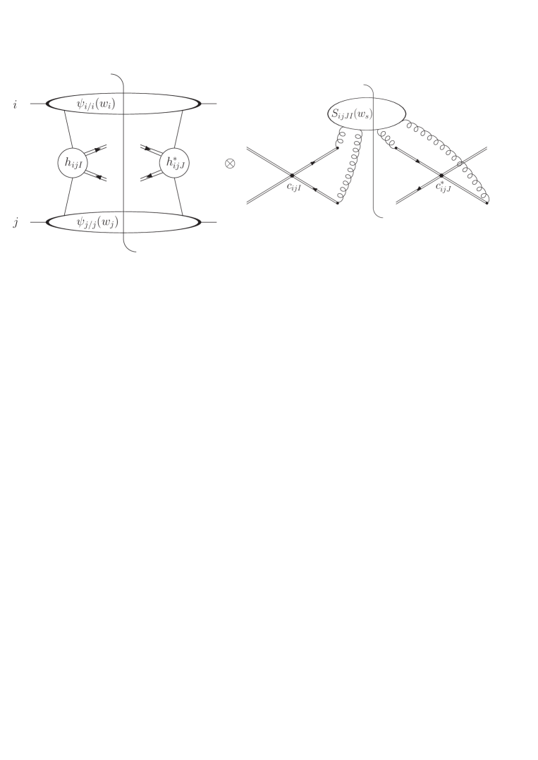
Figure 1: Refactorized form of heavy quark partonic cross section near threshold.

Each of the functions $\psi$, $h$, and $S$ organizes large corrections corresponding to a particular region of phase space. The meaning of the $I,J$ indices will be given shortly and the coefficients $c_{ij\,I}$ are given below in Eq. (3.2). Factorizations of this type have been discussed earlier for deep-inelastic scattering and Drell-Yan production [1], heavy quark hadro- and electroproduction [4, 5, 8, 13], dijet [6] and Higgs [16] production, and single-particle/jet inclusive cross sections [12, 21]. They may be generalized to include recoil effects [37].

Figure 1 indicates that each factorized function depends on its own weight function [3]. In essence, the choice of working in 1PI or PIM kinematics depends on how the total weight $w_{K}$ is constructed from the individual contributions of each weight function [6, 12]:

$${\rm PIM:} \qquad\qquad w_{\rm\scriptstyle PIM}\,=\,w_{i}+w_{j}+w_{s}$$ (26)

$${\rm 1PI:} \qquad\qquad w_{\rm\scriptstyle 1PI}\,=\,w_{i}\left(\frac{-u_{1}}{m^{2}}\right)+w_{j}\left(\frac{-t_{1}}{m^{2}}\right)+w_{s}\,.$$ (27)

In the case of 1PI kinematics it is convenient to define

$${\rm 1PI:} \qquad\qquad N_{u}=N\left(\frac{-u_{1}}{m^{2}}\right),\qquad N_{t}=N\left(\frac{-t_{1}}{m^{2}}\right)\,.$$ (28)

In both kinematics, the moments of the $ij$ partonic cross section, Eqs. (4), (5), (12), and (13), can be written in refactorized form, up to ${\cal O}(1/N)$ corrections, as [4, 5, 6, 12]

$$\tilde{\omega}_{ij}(N,s,t_{1},u_{1},m^{2},\mu^{2},\alpha_{s}(\mu))\; = h^{*}_{ij\,J}(\zeta_{K},m^{2},\mu^{2})\;{\tilde{S}}_{ij\,JI}\!\left({m\over N\mu},\zeta_{K}\right)h_{ij\,I}(\zeta_{K},m^{2},\mu^{2})\;$$ (29)

$$\times\,\left[{{\tilde{\psi}}_{i/i}(N_{u},k_{1}\cdot\zeta_{K}/\mu)\,{\tilde{\psi}}_{j/j}(N_{t},k_{2}\cdot\zeta_{K}/\mu)\over{\tilde{\phi}}_{i/i}(N_{u},\mu)\,{\tilde{\phi}}_{j/j}(N_{t},\mu)}\right]\,.$$

The indices $I$ and $J$ take values in the color-tensor space spanned by the invariant tensors that combine the SU(3) representations of the external partons at threshold into a singlet. The vector $\zeta_{K}^{\mu}$ defines the kinematics, see section 2. The “incoming-jet functions” ${\tilde{\psi}}_{i/i}$ describe the dynamics of partons moving collinearly to the incoming parton $i$. The distributions ${\tilde{\phi}}_{i/i}$ are defined at fixed light-cone momentum while the functions ${\tilde{\psi}}_{i/i}$ are defined at fixed $k_{i}\cdot\zeta_{K}$. The (real) ${\tilde{\psi}}_{i/i}$ functions include all leading and some next-to-leading singular functions and are diagonal in color-tensor space. The function ${\tilde{S}}_{ij\,JI}$, a Hermitian matrix in color-tensor space, summarizes the dynamics of soft gluons that are not collinear to the incoming partons and contains the remaining next-to-leading contributions. Note that (next-to-leading) singularities associated with soft radiation from the outgoing heavy quarks are included in ${\tilde{S}}_{ij\,JI}$ [4, 5]. Finally, the Hermitian matrix $H_{ijIJ}\equiv h_{ijI}h^{*}_{ijJ}$ incorporates the effects of far off-shell partons and contains no singular functions.

The jet and soft functions in Eq. (29) can each be represented as operator matrix elements [4, 5, 6, 7, 12]. The refactorization of the cross section in Eq. (29) can in fact be seen as a separation of near-threshold degrees of freedom into distinct effective field theories [3, 4, 5]. In each effective theory a resummation of the singular functions may be performed via appropriate evolution equations. The resummed cross section is composed of contributions from all these effective theories which must be matched together properly, at a specified scale and to a certain order in perturbation theory. In this paper we match to NLO, leading to NNLL accuracy in our finite order expansions. Our matching scale is the heavy quark mass $m$. The matching procedure is described in section 4.

In the following we describe the resummation of the jet and soft functions. Most of these steps have been discussed previously in the literature [4, 5, 6, 12] so that our description is brief.

3.2 Resummed Jet and Soft Functions

The (exponentiated) $N$ dependence of the ratio ${\tilde{\psi}}_{i/i}/{\tilde{\phi}}_{i/i}$ in Eq. (29) follows from its factorization properties [1, 3]. The function ${\tilde{\psi}}_{i/i}$ obeys, beside a renormalization group equation, an evolution equation governing the energy dependence, expressed as gauge-dependence [1, 3, 38, 39]. Solving these equations leads to the resummed form of this ratio. The function $\psi$ has been defined in PIM kinematics for $i=q$ [1] and $g$ [6] with the 1PI equivalents given in Refs. [13, 12]. The resummation of Sudakov logarithms in 1PI kinematics was verified [13] to trace those in PIM kinematics [1]. Expressed in terms of $w_{i}$, the ${\tilde{\psi}}_{i/i}$ are the same in PIM and 1PI kinematics.

The resummed ratio ${\tilde{\psi}}_{i/i}/{\tilde{\phi}}_{i/i}$ is

$$\ln{\tilde{\psi}_{i/i}\left(N,2k_{i}\cdot\zeta_{K}/\mu\right)\over\tilde{\phi}_{i/i}(N,\mu)}\Big{|}_{\mu=2k_{i}\cdot\zeta_{K}} = \tilde{E}_{i}\left(N,2k_{i}\cdot\zeta_{K}\right)\,,$$ (30)

with the $\overline{\rm MS}$ exponent

$$\tilde{E}_{i}\left(N,2k_{i}\cdot\zeta_{K}\right) = \int\limits^{\infty}_{0}dw\,\frac{(1-e^{-Nw})}{w}\;\Bigg{\{}\int\limits^{1}_{w^{2}}\frac{d\lambda}{\lambda}A_{i}\left[\alpha_{s}(\sqrt{\lambda}\,2k_{i}\cdot\zeta_{K})\right]$$

$$\mbox{}+\frac{1}{2}\nu^{i}\left[\alpha_{s}\left(w\,2k_{i}\cdot\zeta_{K}\right)\right]\,\Bigg{\}}\,.$$

The functions $A_{i}$ and $\nu^{i}$ differ by color factors for $i=q$ and $g$ so that

$$A_{q}(\alpha_{s}) = {\alpha_{s}\over\pi}C_{F}+\left({\alpha_{s}\over\pi}\right)^{2}\left(\frac{1}{2}C_{F}\,K\right)+\ldots,\hskip 14.22636ptA_{g}(\alpha_{s})\;=\;{\alpha_{s}\over\pi}C_{A}+\left({\alpha_{s}\over\pi}\right)^{2}\left(\frac{1}{2}C_{A}\,K\right)+\ldots,$$

$$\nu^{q}\left(\alpha_{s}\right) = \frac{\alpha_{s}}{\pi}(2C_{F})+\ldots,\hskip 99.58464pt\nu^{g}(\alpha_{s})\;=\;\frac{\alpha_{s}}{\pi}(2C_{A})+\ldots,$$ (32)

with $K=C_{A}\;\left({67/18}-{\pi^{2}/6}\right)-{5n_{f}/9}$ [40].

To incorporate the effects of scale changes in finite-order $\alpha_{s}$ expansions, we note that the ratio ${\tilde{\psi}}_{i/i}/{\tilde{\phi}}_{i/i}$ transforms under renormalization scale, $\mu_{R}$, and factorization scale, $\mu$, as

$$\mu_{R}\frac{d}{d\mu_{R}}\ln{\tilde{\psi}_{i/i}\left(N,2k_{i}\cdot\zeta_{K}/\mu_{R}\right)\over\tilde{\phi}_{i/i}(N,\mu)} = \gamma_{\psi_{i}}\;=\;2\gamma_{i}\left(\alpha_{s}(\mu_{R})\right)\,,$$ (33)

$$\mu\frac{d}{d\mu}\ln{\tilde{\psi}_{i/i}\left(N,2k_{i}\cdot\zeta_{K}/\mu_{R}\right)\over\tilde{\phi}_{i/i}(N,\mu)} = -2\gamma_{i/i}\left(N,\alpha_{s}(\mu)\right)\,,$$ (34)

where $\gamma_{i}$ and $2\gamma_{i/i}$ are, respectively, the anomalous dimension of the quantum field $i$ and of the operator whose matrix element represents [41, 42] the $\overline{\rm MS}$-density ${\tilde{\phi}}_{i/i}$. The anomalous dimension for the renormalization scale dependence of $\tilde{\psi}_{i/i}$ [6] in Eq. (33) does not depend on the moment $N$ because the ultraviolet (UV) divergences of $\tilde{\psi}_{i/i}$ are only due to wavefunction renormalization of parton $i$. Hence $\gamma_{\psi_{i}}=2\gamma_{i}$ where $\gamma_{i}$ is calculated in the axial gauge. The anomalous dimension $\gamma_{i/i}$ controlling the factorization scale dependence does depend on $N$. The axial gauge anomalous dimensions are (neglecting ${\cal O}(1/N)$ terms)

$$\gamma_{q}\left(\alpha_{s}\right) = \frac{3}{4}\,C_{F}\,\frac{\alpha_{s}}{\pi}+\ldots\,,$$ (35)

$$\gamma_{q/q}\left(N,\alpha_{s}\right) = -\frac{\alpha_{s}}{\pi}\left(C_{F}\ln N-\frac{3}{4}\,C_{F}\,\right)-\left(\frac{\alpha_{s}}{\pi}\right)^{2}\left(\frac{1}{2}C_{F}K\ln N\right)+\ldots\,,$$ (36)

$$\gamma_{g}\left(\alpha_{s}\right) = b_{2}\,\frac{\alpha_{s}}{\pi}+\ldots\,,$$ (37)

$$\gamma_{g/g}\left(N,\alpha_{s}\right) = -\frac{\alpha_{s}}{\pi}\Biggl{(}C_{A}\ln N-b_{2}\Biggr{)}-\left(\frac{\alpha_{s}}{\pi}\right)^{2}\left(\frac{1}{2}C_{A}K\ln N\right)+\ldots\,,$$ (38)

where $b_{2}$ is given below Eq. (25) and $K$ is given below Eq. (32).

The composite operator [7] that defines ${\tilde{S}}_{ij\,JI}$ contains UV divergences beyond the self energies of its external legs. An additional renormalization removes these extra divergences. However, the product $H_{ijIJ}{\tilde{S}}_{ijJI}$ has no UV divergencies beyond those taken into account by the renormalization of the elementary fields and couplings of the theory, because the renormalization-group invariant cross section and this product only differ by the functions ${\tilde{\psi}}_{i/i}$ which are renormalized as if they were (the “square” of) elementary fields (33). Hence the extra UV divergencies of ${\tilde{S}}_{ijJI}$ are balanced by similar ones in $H_{ijIJ}$. Therefore, the unrenormalized expressions ${\tilde{S}}_{ijJI}^{\rm bare}$ and $H_{ijIJ}^{\rm bare}$ renormalize multiplicatively [4, 5, 6]

$$H^{\rm{bare}}_{ij\,IJ} = Z_{i}^{-1}\,Z_{j}^{-1}\,\Bigl{(}Z_{ij\,S}\Bigr{)}_{IK}^{-1}H_{ij\,KL}\left(Z_{ij\,S}^{{}^{\dagger}}\right)_{LJ}^{-1}\,,$$ (39)

$${\tilde{S}}^{\rm{bare}}_{ij\,JI} = \left(Z_{ij\,S}^{{}^{\dagger}}\right)_{JK}{\tilde{S}}_{ij\,KL}\Bigl{(}Z_{ij\,S}\Bigr{)}_{LI}\,.$$ (40)

The factors $Z_{i}$ denote the renormalization constants of the external fields $i=q,\bar{q},g$. For a given parton pair $ij$, the $(Z_{ij\,S})_{IJ}$ constitute a matrix, in color-tensor space, of renormalization constants for the overall renormalization of the soft function. Note that $(Z_{ij\,S})_{IJ}$ also includes the wave function renormalization of the external heavy quark legs.

Equation (40) leads directly to a renormalization group equation for the matrix $\tilde{S}_{ijJI}$ [4, 5, 6]

$$\mu_{R}\frac{d}{d\mu_{R}}\,{\tilde{S}}_{ij\,JI} = -\Gamma^{ij\,^{\dagger}}_{S,JK}\,{\tilde{S}}_{ij\,KI}-{\tilde{S}}_{ij\,JK}\,\Gamma^{ij}_{S,KI}\,.$$ (41)

The soft anomalous dimension matrix $\Gamma^{ij}_{S,IJ}$ is obtained from the renormalization constants $(Z_{S})_{IJ}$, computed in $d=4-\epsilon$ dimensions, by [43]

$$\Gamma^{ij}_{S,IJ}=-{g_{s}\over 2}{\partial\over\partial g_{s}}{\rm Res_{\epsilon\rightarrow 0}}(Z_{ij\,S})_{IJ}(\alpha_{s},\epsilon)\,.$$ (42)

with $g_{s}^{2}=4\pi\alpha_{s}$. The solution of Eq. (41) is in general expressed in terms of path-ordered exponentials [4, 5, 6], see below.

An explicit expression for $\Gamma^{ij}_{S,IJ}$ requires a choice of basis tensors in color-tensor space. We choose an $s$-channel singlet-octet basis

$$(c_{q\overline{q}\,I})_{mnkl} = \left(\delta_{mn}\delta_{kl}\,,(T^{c}_{F})_{nm}\,(T^{c}_{F})_{kl}\right),$$

$$(c_{gg\,I})_{abkl} = \left(\delta_{ab}\delta_{kl}\,,d_{abc}(T^{c}_{F})_{kl}\,,{\rm{i}}f_{abc}(T^{c}_{F})_{kl}\right)\,,$$ (43)

where $T^{c}_{F}$ are the SU(3) generators in the fundamental representation, where the indices $m,n,k,l$ take values. The indices $a,b,c$ are adjoint indices while $d_{abc}$ and $f_{abc}$ are the totally symmetric and antisymmetric SU(3) invariant tensors, respectively. In this basis, the one-loop soft anomalous dimension matrix for the $q\bar{q}$ process is [4, 5, 22]

$$\Gamma^{q\bar{q}}_{S}=\left[\begin{array}[]{cc}\Gamma^{q\bar{q}}_{11}&\Gamma^{q\bar{q}}_{12}\\ \Gamma^{q\bar{q}}_{21}&\Gamma^{q\bar{q}}_{22}\end{array}\right]\,,$$ (44)

with matrix elements

$$\Gamma^{q\bar{q}}_{11} = -\frac{\alpha_{s}}{\pi}C_{F}\,[L_{\beta}+\ln(2\sqrt{\nu_{1}\nu_{2}})+\pi i]\,,$$

$$\Gamma^{q\bar{q}}_{21} = \frac{2\alpha_{s}}{\pi}\ln\left(\frac{u_{1}}{t_{1}}\right)\,,$$

$$\Gamma^{q\bar{q}}_{12} = \frac{\alpha_{s}}{\pi}\frac{C_{F}}{C_{A}}\ln\left(\frac{u_{1}}{t_{1}}\right)\,,$$

$$\Gamma^{q\bar{q}}_{22} = \frac{\alpha_{s}}{\pi}\left\{C_{F}\left[4\ln\left(\frac{u_{1}}{t_{1}}\right)-\ln(2\sqrt{\nu_{1}\nu_{2}})-L_{\beta}-\pi i\right]\right.$$ (45)

$$\left.{}+\frac{C_{A}}{2}\left[-3\ln\left(\frac{u_{1}}{t_{1}}\right)-\ln\left(\frac{m^{2}s}{t_{1}u_{1}}\right)+L_{\beta}+\pi i\right]\right\}\,.$$

The function $L_{\beta}$ is defined as

$$L_{\beta}=\frac{1-2m^{2}/s}{\beta}\left(\ln\frac{1-\beta}{1+\beta}+\pi i\right)\,.$$ (46)

The variables $\nu_{i},\,i=1,2$ are

$$\nu_{i}=\frac{2(k_{i}\cdot\zeta_{K})^{2}}{s}\,.$$ (47)

The one-loop soft anomalous dimension matrix for the $gg$ process [5, 22] can be written as

$$\Gamma^{gg}_{S}=\left[\begin{array}[]{ccc}\Gamma^{gg}_{11}&0&\frac{1}{2}\Gamma^{gg}_{31}\vspace{2mm}\\ 0&\Gamma^{gg}_{22}&\frac{N_{c}}{4}\Gamma^{gg}_{31}\vspace{2mm}\\ \Gamma^{gg}_{31}&\frac{N_{c}^{2}-4}{4N_{c}}\Gamma^{gg}_{31}&\Gamma^{gg}_{22}\end{array}\right]\,,$$ (48)

where the three independent matrix elements are

$$\Gamma^{gg}_{11} = \frac{\alpha_{s}}{\pi}\left[-C_{F}(L_{\beta}+1)+C_{A}\left(-\frac{1}{2}\ln\left({4\nu_{1}\nu_{2}}\right)+1-\pi i\right)\right],$$ (49)

$$\Gamma^{gg}_{31} = \frac{2\alpha_{s}}{\pi}\ln\left(\frac{u_{1}}{t_{1}}\right)\,,$$

$$\Gamma^{gg}_{22} = \frac{\alpha_{s}}{\pi}\left\{-C_{F}(L_{\beta}+1)+\frac{C_{A}}{2}\left[-\ln\left(4\nu_{1}\nu_{2}\right)+2+\ln\left(\frac{t_{1}u_{1}}{m^{2}s}\right)+L_{\beta}-\pi i\right]\right\}.$$

Note that we did not absorb the function $\nu^{i}$ of Eq. (3.2) into $\Gamma_{S}$.

Combining the solution of Eq. (41) with the resummed jet functions and the hard function, and using matrix notation for $H_{ij}$ and ${\tilde{S}}_{ij}$, the full resummed partonic cross section is

$$\tilde{\omega}^{\rm res}_{ij}(N,s,t_{1},u_{1},m^{2},\mu^{2},\alpha_{s}(\mu))\,=\,{\rm Tr}\Bigg{\{}H_{ij}(\zeta_{K},m^{2},m^{2})$$ (50)

$$\times{\rm\bar{P}}\exp\left[\int_{m}^{m/N}{d\mu^{\prime}\over\mu^{\prime}}(\Gamma^{ij}_{S})^{{}^{\dagger}}\left(\alpha_{s}(\mu^{\prime})\right)\right]{\tilde{S}}_{ij}\!\left(1,\zeta_{K}\right){\rm P}\exp\left[\int_{m}^{m/N}{d\mu^{\prime}\over\mu^{\prime}}\Gamma^{ij}_{S}\left(\alpha_{s}(\mu^{\prime})\right)\right]\Bigg{\}}$$

$$\times\exp\left(\tilde{E}_{i}(N_{u},\mu,\mu_{R})\right)\,\exp\left(\tilde{E}_{j}(N_{t},\mu,\mu_{R})\right)\,\,\exp\Bigg{\{}2\,\int\limits_{\mu_{R}}^{m}{d\mu^{\prime}\over\mu^{\prime}}\,\,\Bigl{(}\gamma_{i}\left(\alpha_{s}(\mu^{\prime})\right)+\gamma_{j}\left(\alpha_{s}(\mu^{\prime})\right)\Bigr{)}\Bigg{\}}\,,$$

where the trace is in color-tensor space, and $\rm P$ refers to path-ordering in $\mu^{\prime}$ such that $\Gamma_{S}^{ij}(\alpha_{s}(m))$ is ordered to the far right while $\Gamma_{S}^{ij}(\alpha_{s}(m/N))$ is ordered to the far left. The operation $\rm\bar{P}$ orders in the opposite way. The exponential $\exp(\tilde{E}_{i})$ is given by

$$\exp(\tilde{E}_{i}(N_{u},\mu,\mu_{R})) = \exp\Bigg{\{}\tilde{E}_{i}\Big{(}N_{u},2k_{i}\cdot\zeta_{K}\Big{)}\Bigg{\}}$$

$$\hskip 8.53581pt\times\exp\Bigg{\{}-2\int\limits_{\mu_{R}}^{2k_{i}\cdot\zeta_{K}}{d\mu^{\prime}\over\mu^{\prime}}\gamma_{i}\left(\alpha_{s}(\mu^{\prime})\right)+2\int\limits_{\mu}^{2k_{i}\cdot\zeta_{K}}{d\mu^{\prime}\over\mu^{\prime}}\gamma_{i/i}\Big{(}N_{u},\alpha_{s}(\mu^{\prime})\Big{)}\Bigg{\}}\,.$$

The exponential $\exp(\tilde{E}_{j})$ is identical except for obvious relabelling. In Eq. (50) we used the renormalization group behaviour, derived from Eqs. (39) and (40), of the product $H_{ij\,IJ}{\tilde{S}}_{ij\,JI}$

$$\mu_{R}\frac{d}{d\mu_{R}}\ln\left[H_{ij\,IJ}(\mu_{R}){\tilde{S}}_{ij\,JI}\!\left(N,\mu_{R}\right)\right] = -2\gamma_{i}\left(\alpha_{s}(\mu_{R})\right)-2\gamma_{j}\left(\alpha_{s}(\mu_{R})\right)\,,$$ (52)

where we have only indicated the $\mu_{R}$ and $N$ dependence. Notice that all $\mu_{R}$ dependence cancels in Eq. (50).

So far, the results have all been given in the $\overline{\rm MS}$-scheme. The $q\overline{q}$ results can also be presented in the DIS scheme, in which the function $\tilde{E}_{q}$ of Eq. (3.2) is

$$\tilde{E}_{q}\left(N,2k_{i}\cdot\zeta_{K}\right)\Biggr{|}_{\rm{DIS}} = \tilde{E}_{q}\left(N,2k_{i}\cdot\zeta_{K}\right)\Biggr{|}_{\rm{\overline{\rm MS}}}+\int\limits^{\infty}_{0}dw\,\frac{(1-e^{-Nw})}{w}\;\Bigg{\{}-\int\limits^{1}_{w}\frac{d\lambda}{\lambda}A_{q}\left[\alpha_{s}(\sqrt{\lambda s})\right]$$ (53)

$$\hskip 128.0374pt\mbox{}{}+g^{{\rm DIS}}_{q}\left[\alpha_{s}(\sqrt{ws})\right]\,\Bigg{\}}\,,$$

with

$$g^{{\rm DIS}}_{q}\left(\alpha_{s}\right)=-\frac{3}{4}\,C_{F}\frac{\alpha_{s}}{\pi}+\ldots\,.$$ (54)

In some cases, e.g. for the unexpanded resummed cross section, it is preferable to diagonalize the matrix $\Gamma^{ij}_{S,IJ}$ [7, 11, 22, 44] by a change of basis in color-tensor space,

$$\Gamma_{R,S}=R^{-1}\,\Gamma_{S}\,R\,,$$ (55)

written in matrix notation with $\Gamma_{R,S}$ diagonal. The channel labels have been suppressed. The columns of the matrix $R$ are the eigenvectors of $\Gamma_{S}$. This leads to ordinary exponentials in the solution of Eq. (41), rather than path-ordered ones. The elements on the diagonal are the (complex) eigenvalues $\lambda_{I}$. In the new basis, indicated by the subscript $R$, the matrices ${\tilde{S}}$ and $H$ are

$${\tilde{S}}_{R}\,=\,R^{{}^{\dagger}}{\tilde{S}}R\,,\,\,\,\,\,\,H_{R}\,=\,R^{-1}H\left(R^{-1}\right)^{{}^{\dagger}}\,,$$ (56)

again in matrix notation. Eq. (41) then becomes

$$\mu\frac{d}{d\mu}\,{\tilde{S}}_{R,JI} = -\left(\lambda_{I}+\lambda^{*}_{J}\right){\tilde{S}}_{R,JI}\,.$$ (57)

The matrix $R_{q{\overline{q}}}$ is given in Refs. [11, 22] while $R_{gg}$ appears in Ref. [22]. The solution of Eq. (57) is

$${\tilde{S}}_{R,JI}\!\left({m\over N\mu},\zeta_{K}\right)\! = \!{\tilde{S}}_{R,JI}\!\left(1,\zeta_{K}\right)\;\exp\left[\,\int\limits_{\mu}^{m/N}{d\mu^{\prime}\over\mu^{\prime}}\!\Bigl{\{}\lambda_{I}(\alpha_{s}(\mu^{\prime}))+\lambda^{*}_{J}(\alpha_{s}(\mu^{\prime}))\Bigr{\}}\right]\,\,\,\,\,\,\,$$ (58)

so that (reinstating the channel labels)

$$\tilde{\omega}^{\rm res}_{ij}(N,s,t_{1},u_{1},m^{2},\mu^{2},\alpha_{s}(\mu))\,=\,\sum\limits_{I,J}\,\,H_{R,ij\,IJ}(\zeta_{K},m^{2},m^{2})$$ (59)

$$\times{\tilde{S}}_{R,ij\,JI}\!\left(1,\zeta_{K}\right)\;\exp\Big{\{}{\tilde{E}_{ij\,JI}}\Big{\}}\,\,\exp\Bigg{[}2\,\int\limits_{\mu}^{m}{d\mu^{\prime}\over\mu^{\prime}}\,\,\Bigl{\{}\gamma_{i}\left(\alpha_{s}(\mu^{\prime})\right)+\gamma_{j}\left(\alpha_{s}(\mu^{\prime})\right)\Bigr{\}}\Bigg{]}\,.$$

The exponential in Eq. (59) carrying color-tensor indices is

$$\exp(\tilde{E}_{ij\,JI}) = \exp(\tilde{E}_{i}(N_{u},\mu,\mu_{R}))\,\exp(\tilde{E}_{j}(N_{t},\mu,\mu_{R}))\,$$

$$\hskip 28.45274pt\times\,\exp\left[\,\int\limits_{m}^{m/N}{d\mu^{\prime}\over\mu^{\prime}}\Bigl{\{}\lambda_{I}(\alpha_{s}(\mu^{\prime}))+\lambda^{*}_{J}(\alpha_{s}(\mu^{\prime}))\Bigr{\}}\right]\,,$$

with $\exp(\tilde{E}_{i})$ and $\exp(\tilde{E}_{j})$ given in Eq. (3.2). We derived the bulk of our subsequent results in both bases.

4 NNLL-NNLO expansions for partonic cross sections

In this section we derive analytical expressions for partonic double-differential heavy quark cross sections up to NNLO by expanding the resummed cross section of the previous section. We concentrate here on the derivation; our explicit results are collected in the appendices. We obtain expressions for both 1PI and PIM kinematics and in both $\overline{\rm MS}$ and DIS factorization schemes. Our aim is NNLL accuracy, as defined in section 2.4, including the scale dependent sector where we distinguish between the renormalization scale $\mu_{R}$ and mass factorization scale $\mu$. This means that for coefficients of $\ln^{i}(\mu^{2}/m^{2})$ or $\ln^{i}(\mu_{R}^{2}/m^{2})$ we include the most singular plus distribution and the two next-most-singular ones.

To achieve NNLL accuracy we must derive NLO matching conditions for certain functions in the resummed cross section, Eq. (50). To this end we expand the factors in this equation and identify order by order the perturbative coefficients of the functions in Eq. (50). The coefficients can in part be explicitly computed and in part inferred by matching to exact NLO results.

4.1 Expansions

Let us expand each factor in Eq. (50) in powers of $\alpha_{s}$. We set $\mu_{R}=m$ here because Eq. (50) is independent of $\mu_{R}$, leading to a cross section expansion in $\alpha_{s}(m)$ which can easily be changed back to $\alpha_{s}(\mu_{R})$. Neglecting $1/N$ terms, the two-loop expansion of $\exp(\tilde{E}_{i})$ may be written as

$$\exp(\tilde{E}_{i}(N_{u},\mu,m))\simeq 1+\frac{\alpha_{s}}{\pi}\left(\sum_{k=0}^{2}C^{i,(1)}_{k}\ln^{k}(N_{u})\right)+\left(\frac{\alpha_{s}}{\pi}\right)^{2}\left(\sum_{k=0}^{4}C^{i,(2)}_{k}\ln^{k}(N_{u})\right)+\ldots$$ (61)

The coefficients $C^{i,(n)}_{k}$ can be computed from the results in section 3. To NNLL accuracy they are

$$C^{i,(1)}_{2} = A_{i}^{(1)},\qquad C^{i,(1)}_{1}=\frac{1}{2}\kappa_{i}+A_{i}^{(1)}l_{\mu},\qquad C^{i,(1)}_{0}=\zeta_{2}C^{i,(1)}_{2}-d_{i}l_{\mu}\,,$$

$$C^{i,(2)}_{4} = \frac{1}{2}\left(A_{i}^{(1)}\right)^{2},\qquad C^{i,(2)}_{3}=\frac{2}{3}b_{2}A_{i}^{(1)}+\frac{1}{2}\kappa_{i}A_{i}^{(1)}+\left(A_{i}^{(1)}\right)^{2}l_{\mu}\,,$$

$$C^{i,(2)}_{2} = A_{i}^{(2)}+\zeta_{2}\left(A_{i}^{(1)}\right)^{2}+\frac{1}{8}\left(\kappa_{i}\right)^{2}+\frac{1}{2}b_{2}\kappa_{i}+\frac{1}{2}\left(A_{i}^{(1)}\right)^{2}l_{\mu}^{2}$$

$$+\mbox{}\frac{1}{2}A_{i}^{(1)}\kappa_{i}l_{\mu}-d_{i}A_{i}^{(1)}l_{\mu}\,,$$

$$C^{i,(2)}_{1} = \left(\zeta_{2}\left(A_{i}^{(1)}\right)^{2}-\frac{1}{2}d_{i}\kappa_{i}+A_{i}^{(2)}\right)l_{\mu}+\left(-\frac{1}{2}b_{2}A_{i}^{(1)}-d_{i}A_{i}^{(1)}\right)l_{\mu}^{2}\,,$$

$$C^{i,(2)}_{0} = \left(\frac{1}{2}b_{2}d_{i}+\frac{1}{2}d_{i}^{2}\right)l_{\mu}^{2}\,,$$ (62)

where we have used the notation

$$\kappa_{i} = \nu^{i,(1)}-2\nu^{i,(1)}\ln\left(\frac{\sqrt{2\nu_{i}s}}{m}\right),\qquad l_{\mu}=\ln\left(\frac{\mu^{2}}{m^{2}}\right)\,,$$

$$d_{q} = \frac{3}{4}C_{F},\qquad d_{g}=b_{2}\,,$$ (63)

and where $A_{i}^{(n)}$ and $\nu^{i,(n)}$ are the coefficients of $(\alpha_{s}/\pi)^{n}$ in the expansion of the functions $A_{i}$ and $\nu^{i}$ in Eq. (32). The two-loop expansion of the path-ordered exponential in Eq. (50) reads

$${\rm P}\exp\left[\int_{m}^{m/N}{d\mu^{\prime}\over\mu^{\prime}}\Gamma_{S}^{ij}\left(\alpha_{s}(\mu^{\prime})\right)\right]_{IJ}\,=\,\delta_{IJ}-\frac{\alpha_{s}(m)}{\pi}\,\ln(N)\Gamma^{ij\,(1)}_{S,IJ}$$ (64)

$$+ \left(\frac{\alpha_{s}(m)}{\pi}\right)^{2}\,\left[\frac{1}{2}\ln^{2}(N)\left[\Gamma^{ij\,(1)}_{S}\times\Gamma^{ij\,(1)}_{S}\right]_{IJ}\,-\,b_{2}\,\ln^{2}(N)\Gamma^{ij\,(1)}_{S,IJ}\right]+\ldots\,,\quad\quad$$

where $\Gamma^{ij\,(1)}_{S}$ is the coefficient of $\alpha_{s}/\pi$ in the one-loop soft anomalous dimensions of Eqs. (44) and (48). The $\bar{\rm P}$ ordered exponential is identical to ${\cal O}(\alpha_{s}^{2})$ up to replacing $\Gamma_{S}$ by $\Gamma_{S}^{{}^{\dagger}}$. The matrices $H_{ij\,IJ}(t_{1},u_{1},m^{2},m^{2})$ and ${\tilde{S}}_{ij\,IJ}\!\left(1,\zeta_{K},\beta_{i},\beta_{j}\right)$ expand to one loop as

$$H_{ij\,IJ} = H^{(0)}_{ij\,IJ}+\frac{\alpha_{s}}{\pi}H^{(1)}_{ij\,IJ}\,,$$

$${\tilde{S}}_{ij\,IJ} = {\tilde{S}}^{(0)}_{ij\,IJ}+\frac{\alpha_{s}}{\pi}{\tilde{S}}^{(1)}_{ij\,IJ}\,.$$ (65)

Let us for the moment choose PIM kinematics by putting $N_{t}=N_{u}=N$. We substitute Eqs. (61), (64), and (4.1) into Eq. (50), finding the moment space expression for the NNLL-NNLO expanded cross section:

$${\tilde{\omega}}_{ij}^{\rm NNLO}(N,s,t_{1},u_{1},m^{2},\mu^{2},\alpha_{s}(\mu))\,=\,{\rm Tr}\left\{H^{(0)}_{ij}{\tilde{S}}^{(0)}_{ij}\right\}$$ (66)

$$+\,\frac{\alpha_{s}}{\pi}\,\Biggl{[}\left((C^{i,(1)}_{2}+C^{j,(1)}_{2})\ln^{2}(N)+(C^{i,(1)}_{1}+C^{j,(1)}_{1})\ln(N)\right)\,{\rm Tr}\left\{H^{(0)}_{ij}{\tilde{S}}^{(0)}_{ij}\right\}$$

$$\hskip 42.67912pt-\ln(N)\,{\rm Tr}\left\{H^{(0)}_{ij}\left(\Gamma^{ij\,(1)}_{S}\right)^{{}^{\dagger}}{\tilde{S}}^{(0)}_{ij}+H^{(0)}_{ij}{\tilde{S}}^{(0)}_{ij}\Gamma^{ij\,(1)}_{S}\right\}$$

$$\hskip 42.67912pt+\,{\rm Tr}\left\{H^{(0)}_{ij}{\tilde{S}}^{(1)}+H^{(1)}{\tilde{S}}^{(0)}_{ij}\right\}+(C^{i,(1)}_{0}+C^{j,(1)}_{0}){\rm Tr}\left\{H^{(0)}_{ij}{\tilde{S}}^{(0)}_{ij}\right\}\Biggr{]}$$

$$+\,\left(\frac{\alpha_{s}}{\pi}\right)^{2}\,\Biggl{[}\Bigg{(}\left(C^{i,(2)}_{4}+C^{j,(2)}_{4}+C^{i,(1)}_{2}C^{j,(1)}_{2}\right)\ln^{4}(N)$$

$$\hskip 14.22636pt+\left(C^{i,(2)}_{3}+C^{j,(2)}_{3}+C^{i,(1)}_{1}C^{j,(1)}_{2}+C^{i,(1)}_{2}C^{j,(1)}_{1}\right)\Bigg{)}\ln^{3}(N)\,{\rm Tr}\left\{H^{(0)}_{ij}{\tilde{S}}^{(0)}_{ij}\right\}$$

$$\hskip 14.22636pt-\left(C^{i,(1)}_{2}+C^{j,(1)}_{2}\right)\ln^{3}(N)\,{\rm Tr}\left\{H^{(0)}_{ij}\left(\Gamma^{ij\,(1)}_{S}\right)^{{}^{\dagger}}{\tilde{S}}^{(0)}_{ij}+H^{(0)}_{ij}{\tilde{S}}^{(0)}_{ij}\Gamma^{ij\,(1)}_{S}\right\}$$

$$\hskip 14.22636pt+\,\ln^{2}(N)\,\left(C^{i,(2)}_{2}+C^{j,(2)}_{2}+\sum_{k=0}^{2}C^{i,(1)}_{k}C^{j,(1)}_{2-k}\right){\rm Tr}\left\{H^{(0)}_{ij}{\tilde{S}}^{(0)}_{ij}\right\}$$

$$\hskip 14.22636pt-(b_{2}+C^{i,(1)}_{1}+C^{j,(1)}_{1})\ln^{2}(N)\,{\rm Tr}\left\{H^{(0)}_{ij}\left(\Gamma^{ij\,(1)}_{S}\right)^{{}^{\dagger}}{\tilde{S}}^{(0)}_{ij}+H^{(0)}_{ij}{\tilde{S}}^{(0)}_{ij}\Gamma^{ij\,(1)}_{S}\right\}$$

$$\hskip 14.22636pt+\,(C^{i,(1)}_{2}+C^{j,(1)}_{2})\ln^{2}(N)\,{\rm Tr}\left\{H^{(0)}_{ij}{\tilde{S}}^{(1)}_{ij}+H^{(1)}_{ij}{\tilde{S}}^{(0)}_{ij}\right\}$$

$$\hskip 14.22636pt+\ln^{2}(N)\,{\rm Tr}\Biggl{\{}\frac{1}{2}H^{(0)}_{ij}\left(\Gamma^{ij\,(1)}_{S}\right)^{{}^{\dagger}}\left(\Gamma^{ij\,(1)}_{S}\right)^{{}^{\dagger}}{\tilde{S}}^{(0)}_{ij}+H^{(0)}_{ij}\left(\Gamma^{ij\,(1)}_{S}\right)^{{}^{\dagger}}{\tilde{S}}^{(0)}_{ij}\Gamma^{ij\,(1)}_{S}$$

$$\hskip 14.22636pt+\frac{1}{2}H^{(0)}_{ij}{\tilde{S}}^{(0)}_{ij}\Gamma^{ij\,(1)}_{S}\Gamma^{ij\,(1)}_{S}\Biggr{\}}\Biggr{]}\,.$$

With 1PI kinematics we use Eq. (28) and expand $\ln(N_{u})=\ln(N)+\ln(-u_{1}/m^{2})$ etc. To transform from moment to momentum space we use results given in the appendices of Refs. [2, 13, 30]. Note that we do not keep subleading terms in our expansions when we invert to momentum space [30].

4.2 Matching

We can identify the functions we must determine from Eq. (66).

The coefficients $C_{k}^{i,(n)}$ are given in Eq. (4.1). The matrices $\Gamma^{ij\,(1)}_{IJ}$ are given in Eqs. (45) and (49). The remaining unknowns are

$$S^{(0)}_{ij\,IJ}\,\,,\;\;H^{(0)}_{ij\,IJ}\,,\;\;{\rm Tr}\left\{H^{(0)}_{ij}{\tilde{S}}^{(1)}_{ij}+H^{(1)}_{ij}{\tilde{S}}^{(0)}_{ij}\right\}\,.$$ (67)

The leading-order soft function ${\tilde{S}}_{IJ}^{(0)}$ is simply

$$\tilde{S}^{(0)}_{ij\,IJ} = {\rm{tr}}\left(c^{{{}^{\dagger}}}_{I}\,c_{J}\right)\,,$$ (68)

where $\{c_{I}\}$ is our basis in color-tensor space. Recall that we have chosen the $s$-channel singlet-octet basis, Eq. (3.2). Note that $\tilde{S}^{(0)}={S}^{(0)}$. The lowest-order hard function $H^{(0)}_{ij\,IJ}=h_{ij\,I}^{(0)}h^{*(0)}_{ij\,J}$ is calculated by projecting the lowest order amplitude ${\cal A}_{ij}$ onto this color basis:

$$h_{ij\,I}^{(0)}\,=\,\left(\tilde{S}^{(0)}_{ij}\right)^{-1}_{IK}\,{\rm{tr}}\left(c^{{{}^{\dagger}}}_{K}\,{\cal A}_{ij}\right)\,,\,\,\,\,\,\,\,\,\,h^{*(0)}_{ij\,J}\,=\,{\rm{tr}}\left({\cal A}_{ij}^{{{}^{\dagger}}}\,c_{K}\right)\,\left(\tilde{S}^{(0)}_{ij}\right)^{-1}_{KJ}\,,$$ (69)

where the trace acts in ordinary color space. Note that at this stage the function $h^{(0)}_{ij\,I}$ may still depend on all other quantum numbers of the process under consideration, such as Lorentz-spinor and spin degrees of freedom. We are however not interested here in spin-dependent observables and we trace over all remaining degrees of freedom. The matrix $H^{(0)}_{ij\,IJ}$ is real and symmetric but may have zero eigenvalues if the Born process does not span the full color-tensor space, as is the case for the $q\bar{q}$ channel. For the $q{\overline{q}}$ channel [11] the results are

$$\tilde{S}^{(0)}_{q{\overline{q}}\,IJ} = \left(\begin{array}[]{cc}N_{c}^{2}&0\\[4.30554pt] 0&\displaystyle\frac{N_{c}^{2}-1}{4}\end{array}\right)\,,\hskip 56.9055ptH^{(0)}_{q{\overline{q}}\,IJ}\,=\,\left(\begin{array}[]{cc}0&0\\ 0&H_{q{\overline{q}}\,22}^{(0)}\end{array}\right)\,,$$ (74)

with $H_{q{\overline{q}}\,22}^{(0)}$ given by

$$H^{(0)}_{q{\overline{q}}\,22}(m,m)\; = \frac{2\pi\,\alpha_{s}^{2}(m)}{N_{c}^{2}}\,\left(\frac{t_{1}^{2}+u_{1}^{2}}{s^{2}}+\frac{2m^{2}}{s}\right)\,.$$ (75)

The lowest-order results are kinematics-independent. For the $gg$ channel we find

$$\tilde{S}^{(0)}_{gg\,IJ} = \left(\begin{array}[]{ccc}N_{c}(N_{c}^{2}-1)&0&0\\[4.30554pt] 0&\displaystyle(N_{c}^{2}-1)\frac{N_{c}^{2}-4}{2N_{c}}&0\\[4.30554pt] 0&0&\displaystyle\frac{1}{2}N_{c}(N_{c}^{2}-1)\end{array}\right)\,,$$ (79)

$$H^{(0)}_{gg\,IJ} = \left(\begin{array}[]{ccc}H^{(0)}_{gg\,11}&N_{c}H^{(0)}_{gg\,11}&H^{(0)}_{gg\,13}\\[4.30554pt] N_{c}H^{(0)}_{gg\,11}&N_{c}^{2}H^{(0)}_{gg\,11}&N_{c}H^{(0)}_{gg\,13}\\[4.30554pt] H^{(0)}_{gg\,13}&N_{c}H^{(0)}_{gg\,13}&H^{(0)}_{gg\,33}\end{array}\right)\,,$$ (83)

where

$$H^{(0)}_{gg\,11}(m,m)\; = \frac{\pi\alpha_{s}^{2}(m)}{2N_{c}^{2}(N_{c}^{2}-1)^{2}}B_{gg}\,,$$ (84)

$$H^{(0)}_{gg\,13}(m,m)\; = \frac{\pi\alpha_{s}^{2}(m)}{2N_{c}(N_{c}^{2}-1)^{2}}B_{gg}\frac{t_{1}^{2}-u_{1}^{2}}{s^{2}}\,,$$ (85)

$$H^{(0)}_{gg\,33}(m,m)\; = \frac{\pi\alpha_{s}^{2}(m)}{2(N_{c}^{2}-1)^{2}}B_{gg}\left(2\frac{t_{1}^{2}+u_{1}^{2}}{s^{2}}-1\right)\,,$$ (86)

and

$$B_{gg} = \frac{u_{1}}{t_{1}}+\frac{t_{1}}{u_{1}}+\frac{4sm^{2}}{t_{1}u_{1}}\left(1-\frac{sm^{2}}{t_{1}u_{1}}\right)\,.$$ (87)

It now remains to determine

$${\rm Tr}\left\{H^{(0)}_{ij}{\tilde{S}}^{(1)}_{ij}+H^{(1)}_{ij}{\tilde{S}}^{(0)}_{ij}\right\}\,.$$ (88)

We do this by matching. The necessary matching conditions can be inferred by comparing the expansion in Eq. (66) to exact results for the partonic cross section.

At lowest order, the matching condition is

$$\tilde{\omega}^{\rm LO}_{ij}(N,s,t_{1},u_{1},m^{2},\mu^{2},\alpha_{s}(\mu))=H^{(0)}_{ij\,IJ}\,\,\tilde{S}^{(0)}_{ij\,JI}\,.$$ (89)

It is straightforward to check that this condition is fulfilled by our results for $\tilde{S}^{(0)}_{ij\,IJ}$ and $H^{(0)}_{ij\,IJ}$. Neglecting $1/N$ terms, and choosing the case $K=\mathrm{PIM}$ for the moment, we have at NLO the matching condition

$$\frac{\alpha_{s}}{\pi}\,\tilde{T}_{ij\,K}^{(1)}\equiv{\rm Tr}\left\{H^{(0)}_{ij}{\tilde{S}}^{(1)}_{ij}+H^{(1)}_{ij}{\tilde{S}}^{(0)}_{ij}\right\}\,=\,\tilde{\omega}^{\rm NLO}_{ij}(N,s,t_{1},u_{1},m^{2},\mu^{2},\alpha_{s}(\mu))$$ (90)

$$-\,\frac{\alpha_{s}}{\pi}\,\Biggl{[}\left((C^{i,(1)}_{2}+C^{j,(1)}_{2})\ln^{2}(N)+(C^{i,(1)}_{1}+C^{j,(1)}_{1})\ln(N)\right)\,{\rm Tr}\left\{H^{(0)}_{ij}{\tilde{S}}^{(0)}_{ij}\right\}$$

$$\hskip 14.22636pt-\ln(N)\,{\rm Tr}\left\{H^{(0)}_{ij}\left(\Gamma^{ij\,(1)}_{S}\right)^{{}^{\dagger}}{\tilde{S}}^{(0)}_{ij}+H^{(0)}_{ij}{\tilde{S}}^{(0)}_{ij}\Gamma^{ij\,(1)}_{S}\right\}+(C^{i,(1)}_{0}+C^{j,(1)}_{0}){\rm Tr}\left\{H^{(0)}_{ij}{\tilde{S}}^{(0)}_{ij}\right\}\Biggr{]}\,.$$

Let us discuss this equation. To begin, the first term on the right hand side may be determined from the exact results in Refs. [32, 33, 34], converted to moment space. To NNLL accuracy this term consists of all terms in the differential one-loop partonic cross sections that either diverge logarithmically or are constant.

The constant terms consist, first of all, of the virtual graph contributions. In addition there is the soft-gluon contribution from the radiative graphs. The virtual contribution is kinematics independent but the soft gluon one is not because what is defined as soft differs for 1PI and PIM kinematics. The respective criteria are $s_{4}<\Delta$ and $1-z<\delta$, with $\Delta$ and $\delta$ defined in Eqs. (22) and (23). The virtual graphs contain various divergences. The ultraviolet ones are cancelled by renormalization of the QCD coupling constant and the heavy quark mass, for both kinematics in the scheme of Ref. [36]. Infrared divergences are cancelled by adding the virtual and soft contributions, so that only collinear divergences remain. These must be subtracted via mass factorization. The corresponding subtraction terms in general involve convolutions of Altarelli-Parisi splitting functions [45] with the lowest order cross section. However, we must mass factorize only with the soft plus virtual parts of these splitting functions. These depend on kinematics, see e.g. Eqs. (6.8) and (6.13) in [32]. What remains at NLO after mass factorization can now be categorized as terms multiplying $\ln^{i}(\Delta/m^{2})$ or $\ln^{i}(\delta)$, $i=1,2$, and other terms. The logarithms $\ln(\Delta/m^{2})$ or $\ln(\delta)$ should be completed to plus-distributions via Eqs. (22) and (23). The final result of these procedures, in moment space, is what constitutes the first term on the right hand side of the equals sign in Eq. (90). The other terms on the right hand side merely subtract all terms containing the singular functions in Eq. (22) or (23).

For 1PI kinematics there is a slight subtlety, related to the use of $N_{t}$ and $N_{u}$ in Eq. (28). Expanding $\ln(N_{t})=\ln(N)+\ln(-t_{1}/m^{2})$ (and $\ln(N_{u})$ likewise) leads to extra terms containing $\ln(-t_{1}/m^{2})$ and $\ln(-u_{1}/m^{2})$ but not $\ln(N)$ and one must be careful in accounting for such terms.

We can now obtain specific results for the matching terms in momentum space. At NLO, $T_{ij\,K}^{(1)}$ on the left hand side of Eq. (90) for 1PI kinematics,

$$T^{(1)}_{ij\,\rm\scriptstyle 1PI}(s,t_{1},u_{1})\equiv\hat{T}^{(1)}_{ij\,\rm\scriptstyle 1PI}(s,t_{1},u_{1})\,\delta(s_{4})\,,$$ (91)

is the expression for $s^{2}d^{2}\sigma^{(1),{\rm S+V}}_{ij}(s,t_{1},u_{1})/dt_{1}\,du_{1}$ given by Eq. (4.7) of Ref. [33] for $ij=q\overline{q}$, and Eq. (6.19) of Ref. [32] for $ij=gg$, modified by removing a factor $\alpha_{s}/\pi$ as well as all terms containing $\ln^{2}(\Delta/m^{2})$ or $\ln(\Delta/m^{2})$ and terms containing $\ln(\mu/m)$ or $\ln(\mu_{R}/m)$. The definition of the hatted symbol in Eq. (91) makes the delta function explicit and is useful when we present the two-loop results.

In PIM kinematics the NLO matching terms may be determined as follows. We start from the above 1PI results and modify those parts that are kinematics dependent. From our discussion following Eq. (90), it is clear that these are only the soft contributions and the mass factorization subtraction terms. We shall label these terms by the superscript ${\rm S\!+\!MF}$. The soft contributions to the PIM NLO cross sections can be computed using the results of Ref. [34]. As mentioned in the above, we mass-factorize these results with only the soft plus virtual part of the splitting functions in PIM kinematics. The same procedure is done for the 1PI case using the results of Refs. [32, 33]. For channel $ij$ we then compute the $\overline{\rm MS}$ quantity

$$\Delta_{ij}^{(1)}(M^{2},{\rm{cos}}\theta)=s\frac{d^{2}\sigma^{(1),{\rm S+MF}}_{ij}(s,M^{2},{\rm{cos}}\theta)}{dM^{2}\,d{\rm{cos}}\theta}\,-\,\frac{\beta}{2}s^{2}\frac{d^{2}\sigma^{(1),{\rm S+MF}}_{ij}(s,t_{1},u_{1})}{dt_{1}\,du_{1}}\Biggr{|}_{\rm PIM}\,$$ (92)

where the subscript PIM on the second term on the right hand side indicates that for $t_{1},u_{1}$ one must use the expressions in Eq. (2.2). Note that we may replace $\beta_{M}$ by $\beta$ to the accuracy at which we are working in this paper, and we shall do so for all following results. Explicit expressions for the terms on the right hand side of Eq. (92) can be found in appendix A. Then the PIM equivalent of Eq. (91) is, accounting for an overall jacobian factor originating from the definition of the cross section,

$$T^{(1)}_{ij\,\rm\scriptstyle PIM}(M^{2},{\rm{cos}}\theta)\equiv\hat{T}^{(1)}_{ij\,\rm\scriptstyle PIM}(M^{2},{\rm{cos}}\theta)\delta(1-z)=\frac{\beta}{2}T^{(1)}_{ij\,\rm\scriptstyle 1PI}(s,t_{1},u_{1})\Biggr{|}_{\rm PIM}+\Delta_{ij}^{(1)}(M^{2},{\rm{cos}}\theta)\,.$$ (93)

Note that terms containing renormalization and factorization scale dependence can be easily included by expanding the corresponding scale dependent exponentials in Eq. (50) and adjusting the coefficients in Eq. (66) correspondingly. Alternatively, the scale dependence can be constructed using renormalization group methods, which we do in the next section.

Changing to the DIS scheme at NNLL for the $q\overline{q}$ channel involves using Eq. (53) rather than Eq. (3.2) in the expansion, Eq. (61), and extra constant terms at NLO as given in appendix B.

Because of their length, we have collected all our results in appendix B. In the next section we perform a numerical study of the results obtained in this section for the inclusive partonic cross sections.

5 Scaling functions

It is convenient to express the inclusive partonic cross sections in terms of dimensionless scaling functions $f^{(k,l)}_{ij}$ that depend only on $\eta$, defined in Eq. (20), as

$$\sigma_{ij}(s,m^{2},\mu^{2}) = \frac{\alpha_{s}^{2}(\mu)}{m^{2}}\sum\limits_{k=0}^{\infty}\,\,\left(4\pi\alpha_{s}(\mu)\right)^{k}\sum\limits_{l=0}^{k}\,\,f^{(k,l)}_{ij}(\eta)\,\,\ln^{l}\left(\frac{\mu^{2}}{m^{2}}\right)\,.$$ (94)

We derive LL, NLL, and NNLL approximations to $f^{(k,l)}_{ij}(\eta)$ for both the $q{\overline{q}}$ and $gg$ channels using the results of the previous section, via Eqs. (8) and (15). Where possible we will compare with exact results. We also examine the results for the $q{\overline{q}}$ channel in the DIS scheme. Of course, a complete comparison between the DIS and ${\overline{\rm{MS}}}$ schemes also requires the use of DIS parton densities, as discussed in the next section.

We begin by showing the scaling functions $f^{(k,0)}_{ij}(\eta),k=0,1,2$, in both 1PI and PIM kinematics. In Fig. 2 we present the $q\overline{q}$ Born and $\overline{\rm MS}$ NLO results for the scaling functions $f^{(0,0)}_{q{\overline{q}}}$ and $f^{(1,0)}_{q{\overline{q}}}$, respectively. A comparison shows that, in the case of $f^{(1,0)}_{q{\overline{q}}}$, the LL approximations already reproduce the exact curve quite well in both kinematics [24], but the NLL approximations agree much better with the exact results to larger $\eta$. Adding the NNLL corrections, numerically dominated by the negative contributions from gluon exchange between final state heavy quarks (Coulomb terms), leads to excellent agreement with the exact curve over a large range of $\eta$. Such progressive improvement was also observed, for 1PI kinematics, in Ref. [46] where the absolute threshold limit was taken. We also see that, while the LL approximations in 1PI and PIM kinematics differ and under- or overestimate the true result, the NLL approximations in both kinematics agree better with each other, and even more so at NNLL, at least for $\eta\;\raisebox{-1.72218pt}{\hbox to0.0pt{$\sim$\hss}}\raisebox{1.72218pt}{$<$}\;0.1$. To summarize the one loop results in this channel, differences due to kinematics choice decrease as the logarithmic accuracy increases.

The same conclusions hold for the NLO scaling function in the $gg$ channel, $f^{(1,0)}_{gg}$, shown in Fig. 3. The Coulomb terms are positive here. At large $\eta$, the agreement between the 1PI and PIM results is not as good as in the $q{\overline{q}}$ channel: the 1PI results at NNLL remain positive while the PIM ones are negative.

Figure 2: (a) The $\eta$-dependence of the scaling functions $f^{(k,0)}_{q{\overline{q}}}(\eta),\;k=0,1$ in the ${\overline{\rm{MS}}}$-scheme and 1PI kinematics. We show the exact results for $f^{(k,0)}_{q{\overline{q}}},\;k=0,1$ (solid lines), the LL approximation to $f^{(1,0)}_{q{\overline{q}}}$ (dotted line), the NLL approximation to $f^{(1,0)}_{q{\overline{q}}}$ (dashed line) and the NNLL approximation to $f^{(1,0)}_{q{\overline{q}}}$ (dashed-dotted line). (b) The same as (a) in PIM kinematics. The spaced-dotted curve corresponds to the approximation involving the leading two powers of $\ln(\beta)$.

Figure 3: (a) The $\eta$-dependence of the scaling functions $f^{(k,0)}_{gg}(\eta),\;k=0,1$ in 1PI kinematics. We show the exact results for $f^{(k,0)}_{gg},\;k=0,1$ (solid lines), the LL approximation to $f^{(1,0)}_{gg}$ (dotted line), the NLL approximation to $f^{(1,0)}_{gg}$ (dashed line) and the the NNLL approximation to $f^{(1,0)}_{gg}$ (dashed-dotted line). (b) The same as (a) in PIM kinematics. The spaced-dotted curve corresponds to the approximation involving the leading two powers of $\ln(\beta)$.

In Figs. 4 and 5, we show the NNLO scaling functions $f^{(2,0)}_{q{\overline{q}}}$ and $f^{(2,0)}_{gg}$ for both kinematics. Again, the LL approximations differ but there is good agreement between 1PI and PIM kinematics at NLL accuracy. We also display the NNLL approximations for $f^{(2,0)}_{q{\overline{q}}}$ and $f^{(2,0)}_{gg}$, presently the best estimates for these functions, at least for $\eta\;\raisebox{-1.72218pt}{\hbox to0.0pt{$\sim$\hss}}\raisebox{1.72218pt}{$<$}1$, since exact calculations are not yet available. Near threshold, the NNLL approximations show some deviation from the NLL approximation due to interplay between the one-loop LL contributions and the one-loop Coulomb terms. Note that while the $q\overline{q}$ channel shows relatively good agreement between the two kinematics at large $\eta$, the $gg$ results are quite different since the 1PI results are positive while the PIM results are negative.

We have also calculated the behavior of the scaling functions $f^{(k,0)}_{ij}(\eta),k=1,2,$ in the threshold limit $s\rightarrow 4m^{2}$, keeping only terms that grow as $\ln(\beta)$ to next-to-leading accuracy. The resulting expressions are given in appendix B.5, and shown in Figs. 2(b), 3(b), 4(b) and 5(b). They agree fairly well with the NLL PIM results.

In general, comparison of the exact and approximate results in the various channels and kinematics in Figs. 2 and 3 indicates the range of $\eta$ values over which we expect the threshold approximation to be valid. The large-$\eta$ behaviour of the scaling functions, furthest away from threshold, may be approximated by the methods of Ref. [47, 48, 49, 50]. However, the behavior of the scaling functions in the intermediate region, $1\;\raisebox{-1.72218pt}{\hbox to0.0pt{$\sim$\hss}}\raisebox{1.72218pt}{$<$}\;\eta\;\raisebox{-1.72218pt}{\hbox to0.0pt{$\sim$\hss}}\raisebox{1.72218pt}{$<$}\;10$, can only be determined by exact computation.

Figure 4: (a) The $\eta$-dependence of the scaling function $f^{(2,0)}_{q{\overline{q}}}(\eta)$ in the ${\overline{\rm{MS}}}$-scheme and 1PI kinematics. We show the LL approximation (dotted line), the NLL approximation (dashed line) and the NNLL approximation (dashed-dotted line). (b) The same as (a) in PIM kinematics. The spaced-dotted curve corresponds to the approximation involving the leading two powers of $\ln(\beta)$.

Figure 5: (a) The $\eta$-dependence of the scaling function $f^{(2,0)}_{gg}(\eta)$ in 1PI kinematics. We show the LL approximation (dotted line), the NLL approximation (dashed line) and the NNLL approximation (dashed-dotted line). (b) The same as (a) in PIM kinematics. The spaced-dotted curve corresponds to the approximation involving the leading two powers of $\ln(\beta)$.

We now check if the $q{\overline{q}}$ ${\overline{\rm{MS}}}$ results are mirrored in the DIS scheme. Since the scaling functions in the two schemes differ already at LL, the higher-order scaling functions will be quite different numerically. Of course, this difference should be compensated in principle by the parton densities for the scheme-independent hadronic cross section.

Figures 6 and 7 show the functions $f^{(1,0)}_{q\overline{q}}$ and $f^{(2,0)}_{q\overline{q}}$ in the DIS scheme. We see again, as in Figs. 2 and 4, that the exact $f^{(1,0)}_{q\overline{q}}$ results are best approximated at small $\eta$ by the NNLL calculations in both kinematics while the LL and NLL calculations either over- or underestimate the exact calculation. The $\overline{\rm MS}$ results generally trace the exact curves somewhat better than those in the DIS scheme. In particular, for the DIS scaling function $f^{(1,0)}_{q{\overline{q}}}$, only the NNLL approximations provide good agreement with the exact curve for both 1PI and PIM kinematics over a large range in $\eta$. This can be traced to the large delta-function terms in the scheme-changing functions in Eqs. (B.1) and (B.3).

Figure 6: (a) The $\eta$-dependence of the scaling function $f^{(1,0)}_{q{\overline{q}}}(\eta)$ in the DIS-scheme and 1PI kinematics. We show the exact result (solid line), the LL approximation (dotted line), the NLL approximation (dashed line) and the NNLL approximation (dashed-dotted line). (b) The same as (a) in PIM kinematics.

Figure 7: (a) The $\eta$-dependence of the scaling function $f^{(2,0)}_{q{\overline{q}}}(\eta)$ in the DIS-scheme and 1PI kinematics. We show the LL approximation (dotted line), the NLL approximation (dashed line) and the NNLL approximation (dashed-dotted line). (b) The same as (a) in PIM kinematics.

We next discuss the functions controlling the scale dependence. They can be determined exactly at NLO and NNLO using renormalization group methods. The exact $f^{(1,0)}_{ij}$ are required to construct $f^{(2,1)}_{ij}$ and $f^{(2,2)}_{ij}$. We neglect flavor mixing terms which are of order $1/N$, where $N$ is the moment variable. We checked that at Tevatron energies the error due to this approximation is less than $1\%$ at NNLO. In this way we obtain

$$f^{(1,1)}_{q{\overline{q}}} = \frac{1}{4\pi^{2}}\left[2b_{2}\,f^{(0,0)}_{q{\overline{q}}}-f^{(0,0)}_{q{\overline{q}}}\otimes P_{qq}^{(0)}\right]\,,$$ (95)

$$f^{(2,1)}_{q{\overline{q}}} \simeq \frac{1}{(4\pi^{2})^{2}}\left[2b_{3}\,f^{(0,0)}_{q{\overline{q}}}-f^{(0,0)}_{q{\overline{q}}}\otimes P_{qq}^{(1)}\right]\,+\frac{1}{4\pi^{2}}\left[3b_{2}\,f^{(1,0)}_{q{\overline{q}}}-f^{(1,0)}_{q{\overline{q}}}\otimes P_{qq}^{(0)}\right]\,,$$ (96)

$$f^{(2,2)}_{q{\overline{q}}} \simeq \frac{1}{(4\pi^{2})^{2}}\left[3b_{2}^{2}\,f^{(0,0)}_{q{\overline{q}}}-\frac{5}{2}b_{2}\,f^{(0,0)}_{q{\overline{q}}}\otimes P_{qq}^{(0)}+\frac{1}{2}f^{(0,0)}_{q{\overline{q}}}\otimes P_{qq}^{(0,0)}\right]\,,$$ (97)

$$f^{(1,1)}_{gg} = \frac{1}{4\pi^{2}}\left[2b_{2}\,f^{(0,0)}_{gg}-f^{(0,0)}_{gg}\otimes P_{gg}^{(0)}\right]\,,$$ (98)

$$f^{(2,1)}_{gg} \simeq \frac{1}{(4\pi^{2})^{2}}\left[2b_{3}\,f^{(0,0)}_{gg}-f^{(0,0)}_{gg}\otimes P_{gg}^{(1)}\right]\,+\frac{1}{4\pi^{2}}\left[3b_{2}\,f^{(1,0)}_{gg}-f^{(1,0)}_{gg}\otimes P_{gg}^{(0)}\right]\,,$$ (99)

$$f^{(2,2)}_{gg} \simeq \frac{1}{(4\pi^{2})^{2}}\left[3b_{2}^{2}\,f^{(0,0)}_{gg}-\frac{5}{2}b_{2}\,f^{(0,0)}_{gg}\otimes P_{gg}^{(0)}+\frac{1}{2}f^{(0,0)}_{gg}\otimes P_{gg}^{(0,0)}\right]\,,$$ (100)

where $P_{qq}^{(0)}$, $P_{gg}^{(0)}$ and $P_{qq}^{(1)}$, $P_{gg}^{(1)}$ are the one- and two-loop splitting functions [51, 41, 52], and $\simeq$ indicates the neglect of flavor-mixing terms. The convolutions involving a scaling function $f^{(i,0)}_{ij}$ are defined as

$$\left(f^{(i,0)}_{pk}\otimes P_{p^{\prime}k}^{(j)}\right)(\eta(x)) \equiv \int\limits_{4m^{2}/s}^{1}\,dz\,\,f^{(i,0)}_{pk}\left(\eta(xz)\right)\,P_{p^{\prime}k}^{(j)}(z)\,$$ (101)

with $\eta(x)=xs/(4m^{2})-1$. The standard convolution of two splitting functions, $P_{qq}^{(0,0)}$ and $P_{gg}^{(0,0)}$, in Eqs. (97) and (100) are

$$P_{ii}^{(0,0)}(x) \equiv \int\limits_{0}^{1}\,dx_{1}\,\int\limits_{0}^{1}\,dx_{2}\,\delta(x-x_{1}x_{2})P_{ii}^{(0)}(x_{1})P_{ii}^{(0)}(x_{2})\,,$$ (102)

with $i=q,g$. Equations (95) and (98) naturally agree with the results for $f^{(1,1)}_{q{\overline{q}}}$ and $f^{(1,1)}_{gg}$ in Ref. [31]. We have also checked that the above results agree to NNLL with the expressions in appendix B when integrated as in Eqs. (8) and (15). Note that in appendix B we have also given results for terms in the differential NNLO functions controlling the scale dependence beyond NNLL accuracy, thus deriving all the soft plus virtual terms in these functions. The exact hard terms are calculated only for the integrated cross section as above.

We begin by showing the scale-changing scaling functions in the $q\overline{q}$ channel and $\overline{\rm MS}$ scheme, comparing 1PI and PIM kinematics. In Fig. 8 we show $f^{(1,1)}_{q{\overline{q}}}$ and note that the PIM LL approximation reproduces the exact curve somewhat better than the 1PI LL aproximation. The NLL approximations agree better, even for larger $\eta$.

Figure 8: (a) The $\eta$-dependence of the scaling function $f^{(1,1)}_{q{\overline{q}}}(\eta)$ in 1PI kinematics. We show the exact result (solid line), the LL approximation (dotted line) and the NLL approximation (dashed line). (b) The same as (a) in PIM kinematics.

Figure 9: (a) The $\eta$-dependence of the scaling functions $f^{(2,1)}_{q{\overline{q}}}(\eta)$ (${\overline{\rm{MS}}}$-scheme) and $f^{(2,1)}_{q{\overline{q}}}(\eta)$ in 1PI kinematics. We show the exact results (solid lines), the LL approximations (dotted lines), the NLL approximations (dashed lines) and the NNLL approximations (dashed-dotted lines). (b) The same as (a) in PIM kinematics.

In Fig. 9 we show the NNLO scaling functions $f^{(2,1)}_{q{\overline{q}}}$ and $f^{(2,2)}_{q{\overline{q}}}$. We compare the exact curves calculated from Eqs. (96) and (97) with our LL, NLL, and NNLL approximations. Again we see that the NNLL approximations provide a remarkably good description of the exact results, both in shape and magnitude. The NNLL curves for 1PI and PIM kinematics are in very good agreement with each other, i.e. ambiguities from the kinematics choice are very mild. Similar conclusions hold for the $gg$ scaling functions $f^{(1,1)}_{gg}$, $f^{(2,1)}_{gg}$, and $f^{(2,2)}_{gg}$, shown in Figs. 10 and 11. Note however that also here the NNLL 1PI and PIM results for $f^{(2,1)}_{gg}$ differ at large $\eta$. The PIM NNLL scaling function differs significantly from the exact result.

Figure 10: (a) The $\eta$-dependence of the scaling function $f^{(1,1)}_{gg}(\eta)$ in 1PI kinematics. We show the exact result (solid line), the LL approximation (dotted line) and the NLL approximation (dashed line). (b) The same as (a) in PIM kinematics; LL and NLL approximation coincide here.

Figure 11: (a) The $\eta$-dependence of the scaling function $f^{(2,l)}_{gg}(\eta),\;l=1,2$ in 1PI kinematics. We show the exact results (solid lines), the LL approximations (dotted lines), the NLL approximations (dashed lines) and the NNLL approximations (dashed-dotted lines). (b) The same as (a) in PIM kinematics.

For completeness, we also display the NNLO scaling functions $f^{(2,1)}_{q{\overline{q}}}$ and $f^{(2,2)}_{q{\overline{q}}}$ in the DIS scheme. The NLL approximations roughly trace the exact curve. The (percentage-wise) large difference between the NLL approximation and the exact curve close to threshold may be attributed to the large constants in the one-loop scheme-changing functions in Eqs. (B.1) and (B.3) that interfere with the one-loop LL terms. These are accounted for at NNLL accuracy, as Fig. 12 demonstrates. However, the NNLL results for $f^{(2,1)}_{q{\overline{q}}}$ differ more significantly between the two kinematic choices than their $\overline{\rm MS}$ counterparts.

Figure 12: (a) The $\eta$-dependence of the scaling function $f^{(2,1)}_{q{\overline{q}}}(\eta)$ in the DIS-scheme and 1PI kinematics. We show the exact result (solid line), the LL approximation (dotted line), the NLL approximation (dashed line) and the NNLL approximation (dashed-dotted line). (b) The same as (a) in PIM kinematics.

6 Hadronic cross sections

In the previous section we examined the quality of our threshold approximations at the parton level. Here we assess these approximations at the hadron level for inclusive top quark production at the Fermilab Tevatron and bottom quark production at HERA-B. The inclusive hadronic cross section is the convolution, Eq. (2.3), of parton distribution functions with the partonic cross section, expressed in terms of the scaling functions, Eq. (94). To facilitate the understanding of the results in this section in terms of those of the previous section, we plot the flux factors $\Phi_{ij}(\eta,\mu^{2})$, Eq. (18), for the above cases in Fig. 13. They show which $\eta$ values receive the most weight in the convolution integral. In our numerical studies we use the two-loop expression of $\alpha_{s}$ and the CTEQ5M ($\overline{\rm MS}$ scheme) or CTEQ5D (DIS scheme) parametrizations of the parton distributions [53] not only for the NLO results, but also for the NNLO (NNLO parton distributions are not yet available) and LO results. Thus in this section we keep the nonperturbative part of our results fixed when studying the effect of increasing the perturbative order of our partonic cross sections. For top quark production at the Tevatron and bottom quark production at HERA-B the calculations probe the moderate to large $x$ region where the parton distributions are well known, see Fig. 13. We use five and four active flavors respectively for these cases and fix $\mu_{R}=\mu$.

Figure 13: (a) The $q\overline{q}$ parton flux factor $\ln(10)\eta/(1+\eta)\Phi_{q{\overline{q}}}$ (see Eq. (2.3)) for the CTEQ5M parametrization at the Tevatron (upper three curves, $\sqrt{S}=1.8$ TeV and $m=175$ GeV) and for HERA-B (lower three curves $\sqrt{S}=41.6$ GeV and $m=4.75$ GeV). We show results for $\mu=m$ (solid curves), $\mu=m/2$ (dotted curves), and $\mu=2m$ (dashed curves). (b) Same as (a) for the $gg$ parton flux factor $\ln(10)\eta/(1+\eta)\Phi_{gg}$. Now the upper set of curves correspond to HERA-B and the lower set to the Tevatron.

Except where specified otherwise we have multiplied the non-exact scaling functions at NLO and NNLO with a damping factor $1/\sqrt{1+\eta}$, as in Ref. [54] in order to lessen the influence of the large $\eta$ region of the scaling functions where threshold logarithms become less dominant and we lose some theoretical control. Figure 14 demonstrates that this factor indeed damps the large $\eta$ region of the NNLO scaling functions $f^{(2,0)}_{ij}$, while leaving the small and medium $\eta$ regions unaffected. The effect of the damping factor will also be made explicit in the tables.

Figure 14: (a) The $\eta$-dependence of the scaling functions $f^{(2,0)}_{q{\overline{q}}}(\eta)$ in the ${\overline{\rm{MS}}}$ scheme with and without the damping factor $1/\sqrt{1+\eta}$. We show the NNLL approximation to $f^{(2,0)}_{q{\overline{q}}}$ in 1PI/PIM kinematics without the factor $1/\sqrt{1+\eta}$ (upper/lower dashed-dotted lines) and with the factor $1/\sqrt{1+\eta}$ (upper/lower boundary of shaded region). The shaded region indicates the residual uncertainty for $f^{(2,0)}_{q{\overline{q}}}$ due to a particular kinematics choice. (b) The same as (a) for $f^{(2,0)}_{gg}(\eta)$.

6.1 Results for $t\bar{t}$ production at the Tevatron

We first discuss top quark production at the Tevatron in proton-antiproton collisions. (For a review of the data see Refs. [55, 56].) We give results for both Run I ($\sqrt{S}=1.8$ TeV) and Run II ($\sqrt{S}=2.0$ TeV). At the Tevatron, top quarks are mainly produced in pairs. With a top quark mass of $175$ GeV, the dominant production channel is $q\bar{q}$ annihilation, constituting about 90% of the total cross section at the Born level for $\sqrt{S}=1.8$ TeV, with the $gg$ channel making up the remainder. The NLO corrections in the $q\bar{q}$ channel are moderate, of the order of 20%, whereas those in the $gg$ channel are more than 80% so that the $gg$ channel gains significance at NLO. These large corrections originate predominantly from the threshold region. Figure 13 shows that the range $0.1\;\raisebox{-1.72218pt}{\hbox to0.0pt{$\sim$\hss}}\raisebox{1.72218pt}{$<$}\;\eta\;\raisebox{-1.72218pt}{\hbox to0.0pt{$\sim$\hss}}\raisebox{1.72218pt}{$<$}\;2$ contributes the most. At still higher orders, this trend continues: the relative corrections to the $gg$ channel are larger than those for the $q{\bar{q}}$ channel, as we shall see. This is due to the larger color factors in the analytical expressions for the corrections for the $gg$ channel. As we mentioned earlier, the $qg$ and $\bar{q}g$ channels give negligible contributions to the total cross section and are not considered here.

We begin by comparing $\overline{\rm MS}$ results in 1PI and PIM kinematics, including only the $q\bar{q}$ channel in Eq. (2.3), at $\sqrt{S}=1.8$ TeV. In Fig. 15 we show the Born cross section and the exact and approximate NLO corrections, the latter at both NLL and NNLL accuracy, for $\mu=m$ in the range $150<m<200$ GeV. We see that our NLO 1PI approximations are a little larger than the exact result while the NLO-NNLL approximation in PIM kinematics is indistinguishable from the exact answer. The corrections are about 20–30% in the mass range shown. In Fig. 16 we give the equivalent results for the $gg$ channel. Here the 1PI approximations agree with the exact result better than the PIM ones.

Figure 17(a) displays the approximate $q{\bar{q}}$ NNLO corrections at NLL and NNLL accuracy for $\mu=m$ as a function of the top quark mass in a direct comparison of the 1PI and PIM results. The shaded area indicates the kinematics ambiguity at NNLL, about 0.6 pb at $m=175$ GeV. The figure shows that the NNLL ambiguity is larger than the NLL one. (Thus the small size of the NLL kinematics ambiguity seems somewhat accidental.) Figure 17(b) shows similar results for the $gg$ channel.

Figure 15: (a) The $q\bar{q}$ channel contribution to the top quark cross section at the Tevatron with $\sqrt{S}=1.8$ TeV and $\mu=m$ in the $\overline{\rm MS}$ scheme. We show the Born term (upper solid line), the exact NLO corrections (lower solid line) and the 1PI approximate NLL (dashed line) and NNLL (dashed-dotted line) one-loop corrections. (b) The same as (a) in PIM kinematics.

Figure 16: (a) The $gg$ channel contribution to the top quark cross section at the Tevatron with $\sqrt{S}=1.8$ TeV and $\mu=m$ in the $\overline{\rm MS}$ scheme. We show the Born term (upper solid line), the exact NLO corrections (lower solid line) and the 1PI approximate NLL (dashed line) and NNLL (dashed-dotted line) one-loop corrections. (b) The same as (a) in PIM kinematics.

Figure 17: (a) The $q\bar{q}$ channel two-loop corrections to the top quark cross section at the Tevatron with $\sqrt{S}=1.8$ TeV and $\mu=m$ in the $\overline{\rm MS}$ scheme. We show the 1PI approximate NLL (upper dashed line) and NNLL (upper boundary of shaded region) two-loop corrections and the PIM approximate NLL (lower dashed line) and NNLL (lower boundary of shaded region) two-loop corrections. (b) The same as (a) for the $gg$ channel two-loop corrections.

For completeness, we show the corresponding results for the $q\bar{q}$ channel in the DIS scheme in Figs. 18 and 19. Again PIM kinematics approximates the exact results somewhat better than 1PI kinematics at NLO-NNLL. We see that the NNLL-NNLO kinematics ambiguity in Fig. 19, again indicated by the shaded region, is greatly reduced compared to the $\overline{\rm MS}$ case, Fig. 17(a). It should however be kept in mind that, in the DIS scheme, the parton densities absorb large threshold logarithms which are not properly accounted for at NNLO if one uses NLO parton distributions as in Fig. 19. Therefore it seems likely that the DIS scheme kinematics ambiguity is somewhat underestimated in Fig. 19.

Figure 18: (a) The $q\bar{q}$ channel contribution to the top quark cross section at the Tevatron with $\sqrt{S}=1.8$ TeV and $\mu=m$ in the DIS scheme. We show the Born term (upper solid line), the exact NLO corrections (lower solid line) and the 1PI approximate NLL (dashed line) and NNLL (dashed-dotted line) one-loop corrections. (b) The same as (a) in PIM kinematics.

Figure 19: The $q\bar{q}$ channel contribution to the top quark cross section at the Tevatron with $\sqrt{S}=1.8$ TeV and $\mu=m$ in the DIS scheme. We show the 1PI approximate NLL (upper dashed line) and NNLL (lower boundary of shaded region) two-loop corrections and the PIM approximate NLL (lower dashed line) and NNLL (upper boundary of shaded region) two-loop corrections.

In Fig. 20 the sum of the $q\bar{q}$ and $gg$ channels in the $\overline{\rm MS}$ scheme is shown as a function of the top quark mass. We display the exact NLO cross section and the approximate NNLO cross section, which is the sum of the exact NLO cross section and the NNLL-NNLO corrections. We show results for $\mu=m/2,m$, and $2m$. We see that the NNLO cross section is uniformly larger than the exact NLO one, although less so in PIM kinematics, and that the scale dependence of the NNLO cross section is considerably reduced relative to NLO. Comparing Figs. 20(a) and (b) we observe that the kinematics ambiguity is larger than the scale uncertainty.

Figure 20: (a) The top quark cross section at the Tevatron with $\sqrt{S}=1.8$ TeV for the sum of the $q\bar{q}$ and $gg$ channels in the $\overline{\rm MS}$ scheme. We show the exact NLO cross section for $\mu=m$ (solid line), $m/2$ (upper dotted line), and $2m$ (lower dotted line), and the 1PI approximate NNLL-NNLO cross section for $\mu=m$ (dashed-dotted line), $m/2$ (upper dashed line), and $2m$ (lower dashed line). (b) The same as (a) in PIM kinematics.

We now turn to a more detailed study of the scale dependence of the inclusive $\overline{\rm MS}$ top cross section. We show the sum of the $q\bar{q}$ and $gg$ channels in Fig. 21 at $\sqrt{S}=1.8$ TeV and $m=$175 GeV at several orders and to different accuracies. The Born and NLO results shown are exact. One of the NNLO curves is constructed by adding the contributions from the NNLL approximate two-loop scaling functions $f^{(2,l)}_{ij},\,l=0,1,2$, to the exact NLO results, the other by adding instead the exact $f^{(2,1)}_{ij}$ and $f^{(2,2)}_{ij}$ functions to the approximate $f^{(2,0)}_{ij}$, thus making the changes to the partonic cross section when changing $\mu$ exact. The differences between these two NNLO curves are due to subleading terms and represent, for each kinematics, the corresponding ambiguity in the scale dependence. At very small $\mu$ the contributions of the terms involving $f^{(2,1)}_{ij}$ and $f^{(2,2)}_{ij}$ are much larger that the contribution from $f^{(2,0)}_{ij}$. The sizable difference between the two NNLO curves in Fig. 21(a) is in fact mainly due to the difference between the exact and NNLL 1PI results for $f^{(2,1)}_{q\overline{q}}$ at medium and large $\eta$ in Fig. 9(a). Even if we include all soft plus virtual terms in the approximate 1PI $f^{(2,1)}_{q\overline{q}}$, as derived in appendix B, there is still a sizeable difference from the exact result. Therefore this difference stems mainly from the hard, i.e. ${\cal O}(1/N)$, terms in $f^{(2,1)}_{q\overline{q}}$.

The NNLO differences in PIM kinematics are much smaller than in 1PI kinematics, in correspondence with the good agreement of the exact and NNLL PIM results for $f^{(2,1)}_{q\overline{q}}$ over all relevant $\eta$, as shown in Fig. 21(b).

Figure 21: (a) The $\mu$-dependence of the top quark cross section at the Tevatron with $\sqrt{S}=1.8$ TeV and $m=175$ GeV for the sum of the $q\bar{q}$ and $gg$ channels in the $\overline{\rm MS}$ scheme. We show the Born (upper solid line at small $\mu/m$) and the exact NLO (lower solid line at small $\mu/m$) cross sections, the 1PI approximate NNLL-NNLO cross section (dashed line) and the NNLO estimate with only $f^{(2,0)}_{q{\overline{q}}}$ and $f^{(2,0)}_{gg}$ NNLL approximate (dashed-dotted line). (b) The same as (a) in PIM kinematics.

Next, in view of the upgrade in energy for the Tevatron from $\sqrt{S}=1.8$ to 2.0 TeV, we investigate the $\sqrt{S}$ dependence of the top quark production cross section. In Fig. 22 we present the inclusive cross section for the sum of the $q\bar{q}$ and $gg$ channels in the $\overline{\rm MS}$ scheme at NLO and NNLO as a function of $\sqrt{S}$. The NNLO curves result from adding the NNLL NNLO corrections to the exact NLO cross section. We have normalized all calculations to the value of the exact NLO cross section at $\mu=m$. Comparing 1PI and PIM kinematics we find that at lower energies, where the $q\bar{q}$ channel is dominant, the NNLO results are 10-30% larger than at NLO in both kinematics. As $\sqrt{S}$ increases, the $gg$ channel, with its larger corrections, grows in importance. The cross sections are also more sensitive to the large $\eta$ behavior of the scaling functions. This leads to large kinematics differences at energies above 5 TeV although the scale uncertainties remain small. In PIM kinematics this is due to $f^{(2,0)}_{gg}$ which is large and negative for $\eta>0.1$ at NNLL, thus reducing the NNLO results relative to the exact NLO cross section.

Figure 22: (a) The top quark cross section with $m=175$ GeV at $p{\bar{p}}$ colliders for the sum of the $q\bar{q}$ and $gg$ channels in the $\overline{\rm MS}$ scheme as a function of $\sqrt{S}$ normalized to the exact NLO cross section at $\mu=m$. We show the ratios of the exact NLO cross sections for $\mu=m$ (solid line), $m/2$ (upper dotted line), and $2m$ (lower dotted line), and the ratios of the 1PI approximate NNLL-NNLO cross sections for $\mu=m$ (dashed-dotted line), $m/2$ (upper dashed line), and $2m$ (lower dashed line). (b) The same as (a) in PIM kinematics.

We now present the values of the NLO and NNLO total $\overline{\rm MS}$ cross sections for top quark production at the Tevatron with $\sqrt{S}=1.8$ TeV and 2.0 TeV for $m=175$ GeV and $\mu=m$, $m/2$, and $2m$ in Tables 1 and 2. They detail the effects of both multiplying the approximate scaling functions $f^{(2,k)}_{ij},\,k=0,1,2$, with the damping factor $1/\sqrt{1+\eta}$ and using the approximate or exact (Eqs. (95)–(100)) scaling functions $f^{(2,1)}_{ij}$ and $f^{(2,2)}_{ij}$ on the NNLO results. Note that all NNLO results in the figures correspond to the option AP+DF, except in Fig. 21 where we also show NNLO results corresponding to the EX+DF choice (dash-dotted lines). Comparing the NNLO and NLO cross sections in the tables shows that the NNLO corrections are much smaller in PIM kinematics than in 1PI kinematics, as already shown in Figs. 22(a) and (b).

$\sqrt{S}=1.8$ TeV
	$\mu=m/2$	$\mu=m$	$\mu=2m$
NLO	5.39	5.16	4.61
NNLO (1PI)
AP	6.27	6.32	6.12
AP+DF	6.19	6.22	5.97
EX	6.91	6.32	5.84
EX+DF	6.73	6.22	5.78
NNLO (PIM)
AP	5.37	5.35	5.26
AP+DF	5.45	5.45	5.29
EX	5.18	5.35	5.26
EX+DF	5.36	5.45	5.31

Table 1: The hadronic $t\overline{t}$ production cross sections in pb for $p\overline{p}$ collisions in the $\overline{\rm MS}$ scheme with $\sqrt{S}=1.8$ TeV and $m=175$ GeV, for $\mu=m,m/2$, and $2m$. The labelling of the NNLO results corresponds to with or without the damping factor (DF) $1/\sqrt{1+\eta}$, and using exact (EX) or NNLL approximate (AP) scaling functions $f^{(2,1)}_{ij}$ and $f^{(2,2)}_{ij}$.

$\sqrt{S}=2.0$ TeV
	$\mu=m/2$	$\mu=m$	$\mu=2m$
NLO	7.37	7.10	6.36
NNLO (1PI)
AP	8.58	8.71	8.46
AP+DF	8.47	8.56	8.24
EX	9.47	8.71	8.06
EX+DF	9.21	8.56	7.97
NNLO (PIM)
AP	7.27	7.27	7.17
AP+DF	7.40	7.43	7.24
EX	6.88	7.27	7.20
EX+DF	7.20	7.43	7.29

Table 2: The hadronic $t\overline{t}$ production cross sections in pb for $p\overline{p}$ collisions in the $\overline{\rm MS}$ scheme with $\sqrt{S}=2.0$ TeV and $m=175$ GeV, for $\mu=m,m/2$, and $2m$. The labelling of the NNLO results corresponds to with or without the damping factor (DF) $1/\sqrt{1+\eta}$, and using exact (EX) or NNLL approximate (AP) scaling functions $f^{(2,1)}_{ij}$ and $f^{(2,2)}_{ij}$.

We see that for the top cross section the effect of the damping factor is rather small. We also note that the use of exact $f^{(2,1)}_{ij}$ and $f^{(2,2)}_{ij}$ affects the $\mu=m/2$ case the most. The difference between the exact and approximate calculation is larger for 1PI than PIM kinematics, as can also be observed in Fig. 21.

We note that AP results in 1PI kinematics were also presented in Ref. [30]. There are some small numerical differences with the results in this paper stemming mainly from using slightly different analytical expressions, all equivalent at threshold. To be specific, the expressions $t_{1}^{2}+u_{1}^{2}$ and $s^{2}-2t_{1}u_{1}$ are equivalent at threshold and either choice can be made in our NNLO expansions. Different choices produce slightly different numerical results away from threshold and the variation in these results represents a small but inherent uncertainty in the cross sections.

Let us finally comment on the applicability of our results for top quark production at the LHC where $\sqrt{S}=14$ TeV. At this $pp$ collider the $gg$ channel is dominant (about 90% of the total) because only sea quarks contribute to the antiquark distributions in the $q\bar{q}$ channel. Although top production at these energies is far from the hadronic threshold region, it might be close enough to partonic threshold for threshold resummation to be relevant since the gluon flux may favor small values of $s=x_{1}x_{2}S\ll S$ (see the discussion in Refs. [57, 58]). Fig. 23 indeed confirms this, but also shows that the hadronic cross section is sensitive to the high-energy behaviour of the scaling functions. Thus, estimates of the inclusive top cross section at the LHC based on the threshold approximation alone are unreliable.

Figure 23: (a) The $q\overline{q}$ parton flux factor, $\ln(10)\eta/(1+\eta)\Phi_{q{\overline{q}}}$, for the CTEQ5M parametrization at the LHC ($\sqrt{S}=14$ TeV and $m=175$ GeV). We show results for $\mu=m$ (solid curve), $\mu=m/2$ (dotted curve), and $\mu=2m$ (dashed curve). (b) Same as (a) for the $gg$ parton flux factor, $\ln(10)\eta/(1+\eta)\Phi_{gg}$.

6.2 Results for $b\bar{b}$ production at HERA-B

In this section we present the inclusive cross section for bottom quark production at fixed-target $pp$ experiments, in particular, the HERA-B experiment. The energy of the proton beam at HERA-B is 920 GeV so that $\sqrt{S}=41.6$ GeV. Here the $gg$ channel is dominant (about 70% of the total cross section), with the $q\bar{q}$ channel contributing the remainder. The $gq$ and $g\bar{q}$ channels are again negligible, of the order of a few percent. Figure 13 shows that the $\eta\;\raisebox{-1.72218pt}{\hbox to0.0pt{$\sim$\hss}}\raisebox{1.72218pt}{$<$}\;1$ region is dominant in the convolution with the parton densities, Eq. (2.3).

In Fig. 24 we present our NLO and NNLL-NNLO results for the $b$ quark production cross section in fixed-target $pp$ interactions as a function of beam energy in the range 200-1200 GeV$/c$ with $m=4.75$ GeV. Comparing 1PI and PIM kinematics we find that, particularly at high energies, the NNLO predictions are different. Again, this can be attributed to increased sensitivity to the high-energy asymptotics of the scaling functions.

Figure 24: (a) The total $\overline{\rm MS}$ bottom quark cross section at fixed-target $pp$ experiments with $m=4.75$ GeV. We show the exact NLO cross section for $\mu=m$ (solid line), $m/2$ (upper dotted line), and $2m$ (lower dotted line), and the NNLL-NNLO cross section for $\mu=m$ (dashed-dotted line), $m/2$ (upper dashed line), and $2m$ (lower dashed line). (b) The same as (a) in PIM kinematics.

$\sqrt{S}=41.6$ GeV
	$\mu=m/2$	$\mu=m$	$\mu=2m$
NLO	31.1	17.8	9.7
NNLO (1PI)
AP	77.1	39.1	21.9
AP+DF	72.2	37.2	20.8
EX	91.1	39.1	20.8
EX+DF	80.7	37.2	20.3
NNLO (PIM)
AP	18.1	19.0	14.0
AP+DF	27.3	21.8	14.7
EX	-19.8	19.0	15.6
EX+DF	-2.5	21.8	16.2

Table 3: The hadronic $b\overline{b}$ production cross sections in nb at HERA-B in the $\overline{\rm MS}$ scheme with $\sqrt{S}=41.6$ GeV and $m=4.75$ GeV for $\mu=m,m/2$, and $2m$. The labelling of the NNLO results corresponds to with or without the damping factor (DF) $1/\sqrt{1+\eta}$, and using exact (EX) or NNLL approximate (AP) scaling functions $f^{(2,1)}_{ij}$ and $f^{(2,2)}_{ij}$.

In Table 3 we list the NLO and NNLO inclusive $b$ quark production cross sections. We show the effects of both using the damping factor $1/\sqrt{1+\eta}$ and the approximate or exact (Eqs. (95)–(100)) scaling functions $f^{(2,1)}_{ij}$ and $f^{(2,2)}_{ij}$ on the NNLO results.

We observe that the damping factor has a significant effect at small scales. The use of exact scaling functions also has a dramatic effect since it causes the NNLO bottom cross section in PIM kinematics to become negative at $\mu=m/2$. The 1PI inclusive cross section at NNLO is significantly larger than the PIM cross section. Only the PIM NNLO results show a significant reduction in scale dependence. Note also that for most options the scale uncertainty is larger than the kinematics ambiguity. In general, we see that the theoretical control over this cross section is still rather poor.

7 Conclusions

In this paper we have resummed threshold enhancements to double-differential heavy quark hadroproduction cross sections, both in single-particle inclusive and pair-invariant mass kinematics and in the $q\bar{q}$ and $gg$ production channels. We used these resummed expressions to construct analytic approximations for the heavy quark cross sections up to NNLO, including the first three powers (NNLL) of the large logarithms. This involved including color-coherence effects and soft radiation attached to all the one-loop virtual corrections, the contribution of which we determined via matching conditions. We derived exact results for the scale-dependent terms at NNLO using renormalization group methods.

We examined the magnitude of the NNLO correction to the inclusive cross section at the parton and hadron levels and studied its variations due to kinematics choice, factorization scheme choice, and changes in the renormalization/factorization scale for top quark production at the Tevatron and bottom quark production at HERA-B. We found that the scale dependence of the cross section after including the NNLO correction is typically substantially reduced, as expected on general grounds [59, 60].

We now provide what are, in our judgement, reasonable values of the approximate NNLO top cross section at 1.8 and 2.0 TeV and the approximate NNLO bottom cross section at 41.6 GeV. These values, based on a combination of the results and their uncertainties, are obtained in the following procedure. For each energy, we take the AP+DF results for each kinematics choice, given in the tables in section 6. The scale uncertainty for 1PI or PIM is given by the maximum and minimum values of the cross sections in each row. The central value of the cross section is the average of the $\mu=m$ values in 1PI and PIM kinematics. Two errors are assigned to the resulting cross section. The first is due to the kinematics-induced ambiguity and is the difference between the central value and the $\mu=m$ values obtained in 1PI and PIM kinematics alone. The second is the weighted average of the scale uncertainties in the two kinematics, giving more weight to smaller scale uncertainties. Thus we obtain the following NNLO top production cross sections at the Tevatron,

$$\sigma_{t\bar{t}}(1.8\,\mathrm{TeV})=5.8\pm 0.4\pm 0.1\;\;\mathrm{pb}\,,$$ (103)

and

$$\sigma_{t\bar{t}}(2.0\,\mathrm{TeV})=8.0\pm 0.6\pm 0.1\;\;\mathrm{pb}\,.$$ (104)

The HERA-B cross section to NNLO is

$$\sigma_{b\bar{b}}(41.6\,\mathrm{GeV})=30\pm 8\pm 10\;\;\mathrm{nb}\,.$$ (105)

Recall that the first set of errors indicates the kinematics ambiguity while the second is an estimate of the scale uncertainty. Note that the scale uncertainty is considerably smaller than the kinematics uncertainty for top production. There are other sources of uncertainties in the total cross section such as parton distribution function uncertainties [61, 62, 63, 64, 65], ambiguities in the analytical expressions near threshold, as discussed in the previous section, and contributions from subleading logarithms [30]. Contributions from even higher orders may also be significant [30]. Due to the relative large uncertainties in the cross section we give one less significant figure in our combined results than in the tables of the previous section.

We note that the central values for the cross sections do not change at all for top production and change only slightly for bottom production if we use any of the other options in the tables. The kinematics uncertainty also changes only slightly for the other options. The scale uncertainty is increased substantially, however, if we use the EX or EX+DF options. The combined results presented here reflect our subjective judgment - more unbiased results are presented in section 6.

In conclusion, we have provided, using soft gluon resummation techniques, improved finite-order perturbative estimates for heavy quark production along with their uncertainties. We hope that our results will thereby allow more meaningful comparisons with measurements.

Acknowledgments

We would like to thank S. Catani, V. Del Duca, J. Owens, J. Smith, G. Sterman, and A. Waldron for fruitful discussions. The work of N.K. is supported in part by the U.S. Department of Energy. The work of E.L. is supported by the Foundation for Fundamental Research of Matter (FOM) and the National Organization for Scientific Research (NWO). The work of S.M. is supported by BMBF under grant BMBF-05HT9VKA and by DFG under contract FOR 264/2-1. The work of R.V. is supported in part by the Division of Nuclear Physics of the Office of High Energy and Nuclear Physics of the U.S. Department of Energy under Contract No. DE-AC-03-76SF00098.

A NNLL matching terms for PIM kinematics

Here we collect the terms required for NLO matching in PIM kinematics. We first define the Born functions that occur in these terms. Recall that in our notation the superscript $(n)$ indicates the power, $(\alpha_{s}(\mu_{R})/\pi)^{n}$, in the expansion of the corresponding quantity.

The $q{\overline{q}}$ channel 1PI Born function is

$$F^{\rm{Born}}_{q\overline{q}}(s,t_{1},u_{1}) = \pi\,\alpha_{s}^{2}(\mu_{R})\,\frac{C_{F}}{N_{c}}\,\left(\frac{t_{1}^{2}+u_{1}^{2}}{s^{2}}+\frac{2m^{2}}{s}\right)\,.$$ (A.1)

The PIM Born function is

$$F^{\rm{Born}}_{q\overline{q}}(s,M^{2},{\rm{cos}}\theta) = \frac{\beta}{2}F^{\rm{Born}}_{q\overline{q}}(s,t_{1},u_{1})|_{\rm\scriptstyle PIM}\,,$$ (A.2)

where the subscript PIM indicates that the expressions for $t_{1}$ and $u_{1}$ in Eq. (2.2) should be used with $\beta_{M}$ replaced by $\beta$.

The $gg$ channel 1PI Born function is

$$F^{\rm{Born}}_{gg}(s,t_{1},u_{1}) = \frac{\alpha_{s}^{2}(\mu_{R})\,\pi}{2(N_{c}^{2}-1)^{2}}\,B_{gg}\,\left[C_{O}\left(1-\frac{2t_{1}u_{1}}{s^{2}}\right)-C_{K}\right]\,,$$ (A.3)

$$B_{gg} = \frac{u_{1}}{t_{1}}+\frac{t_{1}}{u_{1}}+\frac{4sm^{2}}{t_{1}u_{1}}\left(1-\frac{sm^{2}}{t_{1}u_{1}}\right)\,.$$ (A.4)

The color factors $C_{O},C_{K}$ and, for later use, $C_{\rm{QED}}$, are defined as

$$C_{O}\,=\,N_{c}(N_{c}^{2}-1)\,,\,\,\,\,\,\,\,C_{K}\,=\,\frac{N_{c}^{2}-1}{N_{c}}\,,\,\,\,\,\,\,\,C_{\rm{QED}}\,=\,\frac{N_{c}^{4}-1}{N_{c}^{2}}\,.$$ (A.5)

The PIM Born function is

$$F^{\rm{Born}}_{gg}(s,M^{2},{\rm{cos}}\theta) = \frac{\beta}{2}F^{\rm{Born}}_{gg}(s,t_{1},u_{1})|_{\rm\scriptstyle PIM}\,.$$ (A.6)

We again indicate that the expressions in Eq. (2.2) should be used for $t_{1}$ and $u_{1}$ with $\beta_{M}$ replaced by $\beta$. We also define for PIM kinematics

$$B^{\prime}_{gg}=\frac{\beta}{2}B_{gg}\,.$$ (A.7)

Let us now turn to the one-loop ${\rm S+MF}$ cross sections, as defined in section 4. The $\overline{\rm MS}$ scheme 1PI $q\overline{q}$ result is

$$s^{2}\frac{d^{2}\sigma^{(1),{\rm S+MF}}_{q\overline{q}}(s,t_{1},u_{1})}{dt_{1}\,du_{1}}\,=\,F^{\rm{Born}}_{q\overline{q}}(s,t_{1},u_{1})\,\,\delta(s_{4})\,$$

$$\hskip 22.76219pt\times\,\Biggl{[}\left(C_{F}-\frac{C_{A}}{2}\right)\frac{1-2m^{2}/s}{\beta}\left\{2\,{\rm Li}_{2}(x)+2\,{\rm Li}_{2}(-x)+2\ln(x)\ln(1-x^{2})-\ln^{2}(x)-\zeta_{2}\right\}$$

$$\hskip 34.1433pt+\,C_{F}\Biggl{\{}1-{3\over 2}\zeta_{2}+4\ln(x)\ln\left(\frac{t_{1}}{u_{1}}\right)+4{\rm Li}_{2}\left(1-\frac{u_{1}}{xt_{1}}\right)-4{\rm Li}_{2}\left(1-\frac{t_{1}}{xu_{1}}\right)$$

$$\hskip 34.1433pt+{\rm Li}_{2}\left(1-\frac{sm^{2}}{t_{1}u_{1}}\right)+{1\over 2}\ln^{2}\left(\frac{sm^{2}}{t_{1}u_{1}}\right)-{\rm Re}L_{\beta}\Biggr{\}}$$

$$\hskip 34.1433pt+\,{1\over 2}C_{A}\Biggl{\{}-3\ln(x)\ln\left(\frac{t_{1}}{u_{1}}\right)-{1\over 2}\ln^{2}x-3{\rm Li}_{2}\left(1-\frac{u_{1}}{xt_{1}}\right)+3{\rm Li}_{2}\left(1-\frac{t_{1}}{xu_{1}}\right)$$

$$\hskip 34.1433pt-{\rm Li}_{2}\left(1-\frac{sm^{2}}{t_{1}u_{1}}\right)-{1\over 2}\ln^{2}\left(\frac{sm^{2}}{t_{1}u_{1}}\right)+{1\over 2}\ln^{2}\left(\frac{t_{1}}{u_{1}}\right)\Biggr{\}}\Biggr{]}\,$$

with $x\equiv(1-\beta)/(1+\beta)$. The $\overline{\rm MS}$ scheme PIM $q\overline{q}$ result is

$$s\frac{d^{2}\sigma^{(1),{\rm S+MF}}_{q\overline{q}}(s,M^{2},{\rm{cos}}\theta)}{dM^{2}\,d{\rm{cos}}\theta}\,=\,\frac{1}{s}F^{\rm{Born}}_{q\overline{q}}(s,M^{2},{\rm{cos}}\theta)\,\delta(1-z)\,$$

$$\hskip 22.76219pt\times\,\Biggl{[}\left(C_{F}-\frac{C_{A}}{2}\right)\frac{1-2m^{2}/s}{\beta}\Biggl{\{}-{\rm Li}_{2}\left(\frac{2\beta}{1+\beta}\right)+{\rm Li}_{2}\left(\frac{-2\beta}{1-\beta}\right)-\ln(x)\ln\left(\frac{s}{m^{2}}\right)\Biggr{\}}$$

$$\hskip 34.1433pt+C_{F}\Biggl{\{}-\frac{1}{\beta}\ln(x)-\frac{3}{2}\zeta_{2}-4\ln\left(\frac{t_{1}}{u_{1}}\right)\ln\left(\frac{s}{m^{2}}\right)-\ln\left(\frac{s}{m^{2}}\right)+4{\rm Li}_{2}\left(1-\frac{2t_{1}}{s(1-\beta)}\right)$$

$$\hskip 34.1433pt+4{\rm Li}_{2}\left(1-\frac{2t_{1}}{s(1+\beta)}\right)-4{\rm Li}_{2}\left(1-\frac{2u_{1}}{s(1-\beta)}\right)-4{\rm Li}_{2}\left(1-\frac{2u_{1}}{s(1+\beta)}\right)$$

$$\hskip 34.1433pt+4\ln\left(\frac{-2t_{1}}{s(1+\beta)}\right)\ln\left(\frac{-2t_{1}}{s(1-\beta)}\right)-4\ln\left(\frac{-2u_{1}}{s(1+\beta)}\right)\ln\left(\frac{-2u_{1}}{s(1-\beta)}\right)+\frac{1}{2}\ln^{2}\left(\frac{s}{m^{2}}\right)\Biggr{\}}$$

$$\hskip 34.1433pt+C_{A}\,\Biggl{\{}\frac{1}{4}\ln^{2}(x)+2\ln\left(\frac{-t_{1}}{m^{2}}\right)\ln\left(\frac{s}{m^{2}}\right)-\ln\left(\frac{-u_{1}}{m^{2}}\right)\ln\left(\frac{s}{m^{2}}\right)-2\,{\rm Li}_{2}\left(1-\frac{2t_{1}}{s(1-\beta)}\right)$$

$$\hskip 34.1433pt-2\,{\rm Li}_{2}\left(1-\frac{2t_{1}}{s(1+\beta)}\right)+{\rm Li}_{2}\left(1-\frac{2u_{1}}{s(1-\beta)}\right)+{\rm Li}_{2}\left(1-\frac{2u_{1}}{s(1+\beta)}\right)$$

$$\hskip 34.1433pt+\ln\left(\frac{-2u_{1}}{s(1+\beta)}\right)\ln\left(\frac{-2u_{1}}{s(1-\beta)}\right)-2\ln\left(\frac{-2t_{1}}{s(1+\beta)}\right)\ln\left(\frac{-2t_{1}}{s(1-\beta)}\right)-\frac{1}{2}\ln^{2}\left(\frac{s}{m^{2}}\right)\Biggr{\}}\Biggr{]}\,.$$

The $\overline{\rm MS}$ scheme 1PI $gg$ result is

$$s^{2}\frac{d^{2}\sigma^{(1),{\rm S+MF}}_{gg}(s,t_{1},u_{1})}{dt_{1}\,du_{1}}\,=\,\frac{\alpha_{s}^{2}(\mu_{R})\pi}{2(N_{c}^{2}-1)^{2}}B_{gg}\,\delta(s_{4})\,$$

$$\hskip 22.76219pt\times\,\Biggl{[}{1\over 2}\left(C_{\rm QED}-N_{c}C_{K}\left(1-\frac{2t_{1}u_{1}}{s^{2}}\right)\right)\frac{1-2m^{2}/s}{\beta}\left\{2\,{\rm Li}_{2}(x)+2\,{\rm Li}_{2}(-x)\right.$$

$$\hskip 51.21495pt\left.+2\ln(x)\ln(1-x^{2})-\ln^{2}(x)-\zeta_{2}\right\}+{1\over 2}C_{\rm QED}\left\{1-{\rm Re}L_{\beta}\right\}$$

$$\hskip 34.1433pt+{1\over 2}N_{c}C_{O}\Biggl{\{}\left(1-\frac{2t_{1}u_{1}}{s^{2}}\right)\left(1-{\rm Re}L_{\beta}-3\zeta_{2}-{1\over 2}\ln^{2}(x)+{1\over 2}\ln^{2}\left(\frac{t_{1}}{u_{1}}\right)+{\rm Li}_{2}\left(1-\frac{sm^{2}}{t_{1}u_{1}}\right)\right.$$

$$\hskip 51.21495pt\left.+{1\over 2}\ln^{2}\left(\frac{sm^{2}}{t_{1}u_{1}}\right)\right)+\frac{(t_{1}^{2}-u_{1}^{2})}{s^{2}}\left(\ln(x)\ln\left(\frac{t_{1}}{u_{1}}\right)+{\rm Li}_{2}\left(1-\frac{u_{1}}{xt_{1}}\right)-{\rm Li}_{2}\left(1-\frac{t_{1}}{xu_{1}}\right)\right)\Biggr{\}}$$

$$\hskip 34.1433pt+{1\over 2}N_{c}C_{K}\Biggl{\{}-2+2{\rm Re}L_{\beta}+3\zeta_{2}+\ln^{2}(x)-\ln^{2}\left(\frac{t_{1}}{u_{1}}\right)-\left(1-\frac{2t_{1}u_{1}}{s^{2}}\right)\left(1-{\rm Re}L_{\beta}\right)\Biggr{\}}\Biggr{]}\,.$$

The $\overline{\rm MS}$ scheme PIM $gg$ result is

$$s\frac{d^{2}\sigma^{(1),{\rm S+MF}}_{gg}(s,M^{2},{\rm{cos}}\theta)}{dM^{2}\,d{\rm{cos}}\theta}\,=\,\frac{1}{s}\frac{\alpha_{s}^{2}(\mu_{R})\pi}{2(N_{c}^{2}-1)^{2}}B^{\prime}_{gg}\,\delta(1-z)\,$$

$$\hskip 22.76219pt\times\,\Biggl{[}{1\over 2}\left(C_{\rm QED}-N_{c}C_{K}\left(1-\frac{2t_{1}u_{1}}{s^{2}}\right)\right)\frac{1-2m^{2}/s}{\beta}\Biggl{\{}-{\rm Li}_{2}\left(\frac{2\beta}{1+\beta}\right)+{\rm Li}_{2}\left(\frac{-2\beta}{1-\beta}\right)$$

$$\hskip 34.1433pt-\ln(x)\ln\left(\frac{s}{m^{2}}\right)\Biggr{\}}+\frac{1}{2}C_{\rm QED}\,\Biggl{(}-\frac{1}{\beta}\ln x-\ln\left(\frac{s}{m^{2}}\right)\Biggr{)}$$

$$\hskip 34.1433pt+\frac{1}{2}N_{c}C_{O}\,\Biggl{\{}\left(1-2\frac{t_{1}u_{1}}{s^{2}}\right)\Biggl{(}-\frac{1}{\beta}\ln(x)-3\zeta_{2}+\frac{1}{2}\ln^{2}(x)+\ln\left(\frac{t_{1}u_{1}}{m^{4}}\right)\ln\left(\frac{s}{m^{2}}\right)$$

$$\hskip 34.1433pt-\ln\left(\frac{s}{m^{2}}\right)\Biggr{)}-\frac{(t_{1}^{2}-u_{1}^{2})}{s^{2}}\ln\left(\frac{t_{1}}{u_{1}}\right)\ln\left(\frac{s}{m^{2}}\right)-2\frac{u_{1}^{2}}{s^{2}}{\rm Li}_{2}\left(1-\frac{2t_{1}}{s(1-\beta)}\right)$$

$$\hskip 34.1433pt-2\frac{u_{1}^{2}}{s^{2}}{\rm Li}_{2}\left(1-\frac{2t_{1}}{s(1+\beta)}\right)-2\frac{t_{1}^{2}}{s^{2}}{\rm Li}_{2}\left(1-\frac{2u_{1}}{s(1-\beta)}\right)-2\frac{t_{1}^{2}}{s^{2}}{\rm Li}_{2}\left(1-\frac{2u_{1}}{s(1+\beta)}\right)$$

$$\hskip 34.1433pt-2\frac{u_{1}^{2}}{s^{2}}\ln\left(\frac{-2t_{1}}{s(1+\beta)}\right)\ln\left(\frac{-2t_{1}}{s(1-\beta)}\right)-2\frac{t_{1}^{2}}{s^{2}}\ln\left(\frac{-2u_{1}}{s(1+\beta)}\right)\ln\left(\frac{-2u_{1}}{s(1-\beta)}\right)\Biggr{\}}$$

$$\hskip 34.1433pt+\frac{1}{2}N_{c}C_{K}\,\Biggl{\{}2\frac{1}{\beta}\ln(x)+3\zeta_{2}-\ln^{2}(x)-2\ln\left(\frac{t_{1}u_{1}}{m^{4}}\right)\ln\left(\frac{s}{m^{2}}\right)+2\ln\left(\frac{s}{m^{2}}\right)+\ln^{2}\left(\frac{s}{m^{2}}\right)$$

$$\hskip 34.1433pt+2\,{\rm Li}_{2}\left(1-\frac{2t_{1}}{s(1-\beta)}\right)+2\,{\rm Li}_{2}\left(1-\frac{2t_{1}}{s(1+\beta)}\right)+2\,{\rm Li}_{2}\left(1-\frac{2u_{1}}{s(1-\beta)}\right)$$

$$\hskip 34.1433pt+2\,{\rm Li}_{2}\left(1-\frac{2u_{1}}{s(1+\beta)}\right)+2\ln\left(\frac{-2t_{1}}{s(1+\beta)}\right)\ln\left(\frac{-2t_{1}}{s(1-\beta)}\right)$$

$$\hskip 34.1433pt+2\ln\left(\frac{-2u_{1}}{s(1+\beta)}\right)\ln\left(\frac{-2u_{1}}{s(1-\beta)}\right)+\left(1-2\frac{t_{1}u_{1}}{s^{2}}\right)\left(\frac{1}{\beta}\ln(x)+\ln\left(\frac{s}{m^{2}}\right)\right)\Biggr{\}}\Biggr{]}\,.$$

B NNLL differential partonic heavy quark cross sections to NNLO

In this appendix we collect all our results for the NNLL-NNLO differential partonic heavy quark cross sections. We first make some general observations. The NLO 1PI results agree with those in Refs. [32, 33, 54]. The NLO PIM results are consistent with Ref. [34]. The $q{\overline{q}}$ channel results contain terms that are antisymmetric under $t_{1},u_{1}$ interchange, a consequence of charge conjugation asymmetry of the initial state. The $gg$ channel results are symmetric under $t_{1}\leftrightarrow u_{1}$. In the $q{\overline{q}}$ channel the Born function factors out as a whole for LL and NLL terms. In the $gg$ channel the Born function function factors out as a whole only for LL terms. We also use the notation that the superscript $(n)$ denotes the coefficient of $(\alpha_{s}(\mu_{R})/\pi)^{n}$ in the expansion of the corresponding quantity.

B.1 The $q{\overline{q}}$ channel in 1PI kinematics

In the $q{\bar{q}}$ channel, Eq. (4), the Born cross section is

$$s^{2}\frac{d^{2}\sigma^{(0)}_{q\overline{q}}(s,t_{1},u_{1})}{dt_{1}\,du_{1}}=\omega^{(0)}_{q\overline{q}}(s,t_{1},u_{1}) = \delta(s+t_{1}+u_{1})\,F^{\rm{Born}}_{q\overline{q}}(s,t_{1},u_{1})\,$$ (B.1)

with $F^{\rm{Born}}_{q\overline{q}}(s,t_{1},u_{1})$ given in Eq. (A.1). The $\overline{\rm MS}$ one-loop NNLL corrections are

$$s^{2}\frac{d^{2}\sigma^{(1)}_{q\overline{q}}(s,t_{1},u_{1})}{dt_{1}\,du_{1}}=\omega^{(1)}_{q\overline{q}}(s_{4},s,t_{1},u_{1})\,=\,F^{\rm{Born}}_{q\overline{q}}(s,t_{1},u_{1})\,\,$$

$$\hskip 22.76219pt\times\,\Biggl{[}\,4C_{F}\,\left[{\ln(s_{4}/m^{2})\over s_{4}}\right]_{+}$$

$$\hskip 34.1433pt{}+\left[1\over s_{4}\right]_{+}\Biggl{\{}2C_{F}\,\left(4\ln\left(\frac{u_{1}}{t_{1}}\right)+\ln\left(\frac{sm^{2}}{t_{1}u_{1}}\right)-{\rm{Re}}L_{\beta}-1-\ln\left(\frac{\mu^{2}}{m^{2}}\right)\right)$$

$$\hskip 62.59605pt+\,C_{A}\left(-3\ln\left(\frac{u_{1}}{t_{1}}\right)-\ln\left(\frac{sm^{2}}{t_{1}u_{1}}\right)+{\rm{Re}}L_{\beta}\right)\Biggr{\}}$$

$$\hskip 8.53581pt{}+\,\delta(s_{4})\,\Biggl{\{}C_{F}\,\ln\left(\frac{\mu^{2}}{m^{2}}\right)\Biggl{(}\ln\left(\frac{t_{1}u_{1}}{m^{4}}\right)-\frac{3}{2}\Biggr{)}+2\ln\left(\frac{\mu_{R}^{2}}{m^{2}}\right)b_{2}\Biggr{\}}\Biggr{]}+\,\,T^{(1)}_{q\overline{q}\,\rm\scriptstyle 1PI}(s,t_{1},u_{1})\,.$$

The $\overline{\rm MS}$ two-loop NLL corrections are

$$s^{2}\frac{d^{2}\sigma^{(2)}_{q\overline{q}}(s,t_{1},u_{1})}{dt_{1}\,du_{1}}=\omega^{(2)}_{q\overline{q}}(s_{4},s,t_{1},u_{1})\,=\,F^{\rm{Born}}_{q\overline{q}}(s,t_{1},u_{1})\,\,$$

$$\hskip 22.76219pt\times\,\Biggl{[}\,8C_{F}^{2}\,\left[{\ln^{3}(s_{4}/m^{2})\over s_{4}}\right]_{+}\,$$

$$\hskip 34.1433pt{}+\left[{\ln^{2}(s_{4}/m^{2})\over s_{4}}\right]_{+}\Biggl{\{}12C_{F}^{2}\left(4\ln\left(\frac{u_{1}}{t_{1}}\right)+\ln\left(\frac{sm^{2}}{t_{1}u_{1}}\right)-{\rm{Re}}L_{\beta}-1\right.$$

$$\hskip 59.75078pt\left.{}-\ln\left(\frac{\mu^{2}}{m^{2}}\right)\right)-4C_{F}b_{2}+6C_{A}C_{F}\left(-3\ln\left(\frac{u_{1}}{t_{1}}\right)-\ln\left(\frac{sm^{2}}{t_{1}u_{1}}\right)+{\rm{Re}}L_{\beta}\right)\Biggr{\}}$$

$$\hskip 34.1433pt+\left[{\ln(s_{4}/m^{2})\over s_{4}}\right]_{+}\Biggl{\{}4C_{F}^{2}\ln\left(\frac{\mu^{2}}{m^{2}}\right)\Biggl{(}\ln\left(\frac{t_{1}u_{1}}{m^{4}}\right)$$

$$\hskip 59.75078pt\left.{}-8\ln\left(\frac{u_{1}}{t_{1}}\right)-2\ln\left(\frac{sm^{2}}{t_{1}u_{1}}\right)+2{\rm{Re}}L_{\beta}+\frac{1}{2}+\ln\left(\frac{\mu^{2}}{m^{2}}\right)\right)+12\ln\left(\frac{\mu_{R}^{2}}{m^{2}}\right)C_{F}b_{2}$$

$$\hskip 59.75078pt{}+4C_{A}C_{F}\ln\left(\frac{\mu^{2}}{m^{2}}\right)\left(3\ln\left(\frac{u_{1}}{t_{1}}\right)+\ln\left(\frac{sm^{2}}{t_{1}u_{1}}\right)-{\rm{Re}}L_{\beta}\right)\Biggr{\}}$$

$$\hskip 34.1433pt{}+\left[{1\over s_{4}}\right]_{+}\ln\left(\frac{\mu^{2}}{m^{2}}\right)\Biggl{\{}\ln\left(\frac{\mu^{2}}{m^{2}}\right)\Biggl{(}C_{F}b_{2}+3C_{F}^{2}-2C_{F}^{2}\ln\left(\frac{t_{1}u_{1}}{m^{4}}\right)\Biggr{)}{}-6\ln\left(\frac{\mu_{R}^{2}}{m^{2}}\right)C_{F}b_{2}\Biggr{\}}\Biggr{]}\,.$$

To achieve NNLL accuracy one must add

$$2\,C_{F}\,\hat{T}^{(1)}_{q\overline{q}\,\rm\scriptstyle 1PI}(s,t_{1},u_{1})\Biggl{\{}2\left[{\ln(s_{4}/m^{2})\over s_{4}}\right]_{+}-\left[{1\over s_{4}}\right]_{+}\ln\left(\frac{\mu^{2}}{m^{2}}\right)\Biggr{\}}\,+\,F^{\rm{Born}}_{q\overline{q}}(s,t_{1},u_{1})$$

$$\hskip 17.07164pt\times\,\Biggl{[}\left[{\ln(s_{4}/m^{2})\over s_{4}}\right]_{+}\Biggl{\{}2C_{F}K+4C_{F}b_{2}\ln\left(\frac{t_{1}u_{1}}{m^{4}}\right)-16C_{F}^{2}\zeta_{2}+4C_{F}^{2}\ln^{2}\left(\frac{t_{1}u_{1}}{m^{4}}\right)$$

$$\hskip 59.75078pt-8C_{F}\left({\rm{Re}}\Gamma^{(1)}_{22}-C_{F}+C_{F}\ln\left(2\sqrt{\nu_{1}\nu_{2}}\frac{s}{m^{2}}\right)\right)\left(\ln\left(\frac{t_{1}u_{1}}{m^{4}}\right)+\frac{1}{2C_{F}}b_{2}\right)$$

$$\hskip 59.75078pt{}+4\Gamma^{(1)}_{12}\Gamma^{(1)}_{21}{}+4\left({\rm{Re}}\Gamma^{(1)}_{22}-C_{F}+C_{F}\ln\left(2\sqrt{\nu_{1}\nu_{2}}\frac{s}{m^{2}}\right)\right)^{2}\Biggr{\}}\,$$

$$\hskip 34.1433pt+\left[{1\over s_{4}}\right]_{+}\ln\left(\frac{\mu^{2}}{m^{2}}\right)\Biggl{\{}-C_{F}K+8C_{F}^{2}\zeta_{2}+3C_{F}^{2}\ln\left(\frac{t_{1}u_{1}}{m^{4}}\right)-2C_{F}^{2}\ln^{2}\left(\frac{t_{1}u_{1}}{m^{4}}\right)$$

$$\hskip 59.75078pt-3C_{F}\left({\rm{Re}}\Gamma^{(1)}_{22}-C_{F}+C_{F}\ln\left(2\sqrt{\nu_{1}\nu_{2}}\frac{s}{m^{2}}\right)\right)$$

$$\hskip 59.75078pt+2C_{F}\ln\left(\frac{t_{1}u_{1}}{m^{4}}\right)\left({\rm{Re}}\Gamma^{(1)}_{22}-C_{F}+C_{F}\ln\left(2\sqrt{\nu_{1}\nu_{2}}\frac{s}{m^{2}}\right)\right)\Biggr{\}}$$

$$\hskip 34.1433pt+\left[{1\over s_{4}}\right]_{+}\ln\left(\frac{\mu_{R}^{2}}{m^{2}}\right)\Biggl{\{}6b_{2}\left({\rm{Re}}\Gamma^{(1)}_{22}-C_{F}+C_{F}\ln\left(2\sqrt{\nu_{1}\nu_{2}}\frac{s}{m^{2}}\right)\right)-6C_{F}b_{2}\ln\left(\frac{t_{1}u_{1}}{m^{4}}\right)\Biggr{\}}$$

$$\hskip 34.1433pt+\delta(s_{4})\Biggl{\{}\ln^{2}\left(\frac{\mu^{2}}{m^{2}}\right)\Biggl{(}-2C_{F}^{2}\zeta_{2}+\frac{3}{4}C_{F}b_{2}+\frac{9}{8}C_{F}^{2}-\frac{1}{2}C_{F}b_{2}\ln\left(\frac{t_{1}u_{1}}{m^{4}}\right)-\frac{3}{2}C_{F}^{2}\ln\left(\frac{t_{1}u_{1}}{m^{4}}\right)$$

$$\hskip 59.75078pt+\frac{1}{2}C_{F}^{2}\ln^{2}\left(\frac{t_{1}u_{1}}{m^{4}}\right)\Biggr{)}+\ln\left(\frac{\mu_{R}^{2}}{m^{2}}\right)\ln\left(\frac{\mu^{2}}{m^{2}}\right)\Biggl{(}-\frac{9}{2}C_{F}b_{2}+3C_{F}b_{2}\ln\left(\frac{t_{1}u_{1}}{m^{4}}\right)\Biggr{)}$$

$$\hskip 59.75078pt+3b_{2}^{2}\ln^{2}\left(\frac{\mu_{R}^{2}}{m^{2}}\right)\Biggr{\}}\Biggr{]}\,$$ (B.4)

where we suppressed the $q\overline{q}$ channel label on the soft anomalous dimension matrix elements.

We note that at NNLL accuracy we have derived all NNLO soft plus virtual terms involving the scale, except for $\delta(s_{4})$ terms involving single logarithms of the scale. We can go beyond NNLL accuracy and also derive these terms in the partonic cross section by requiring that the scale dependence in the hadronic cross section cancel out. These terms are

$$F^{\rm{Born}}_{q\overline{q}}(s,t_{1},u_{1})\delta(s_{4})\left\{\ln\left(\frac{\mu_{R}^{2}}{m^{2}}\right)\left[\frac{b_{3}}{128}+\frac{3}{16}b_{2}{\hat{T^{\prime}}}^{(1)}_{q{\bar{q}}\,\rm 1PI}(s,t_{1},u_{1})\right]\right.$$

$${}+\ln\left(\frac{\mu_{F}^{2}}{m^{2}}\right)\left[-8C_{F}^{2}\zeta_{3}+4C_{F}\zeta_{2}\left({\rm Re}{\Gamma}_{22}^{(1)}-C_{F}+C_{F}\ln(2\sqrt{\nu_{1}\nu_{2}})-C_{F}\ln\left(\frac{t_{1}u_{1}}{sm^{2}}\right)\right)\right.$$ (B.5)

$$\hskip 56.9055pt\left.\left.{}+C_{F}\left(\ln\left(\frac{t_{1}u_{1}}{m^{4}}\right)-\frac{3}{2}\right){\hat{T^{\prime}}}^{(1)}_{q{\bar{q}}\,\rm 1PI}(s,t_{1},u_{1})+\frac{1}{2}C_{F}K\ln\left(\frac{t_{1}u_{1}}{m^{4}}\right)\right]\right\}\,,$$

with ${\hat{T^{\prime}}}^{(1)}_{q{\bar{q}}\,\rm 1PI}(s,t_{1},u_{1})={\hat{T}}^{(1)}_{q{\bar{q}}\,\rm 1PI}(s,t_{1},u_{1})/F^{\rm{Born}}_{q\overline{q}}(s,t_{1},u_{1})$. We have checked that these results are consistent with the exact expressions in Eq. (96) and with the expansion of the resummed cross section beyond NNLL accuracy as discussed in Ref. [30].

The DIS one-loop NNLL corrections are

$$s^{2}\frac{d^{2}\sigma^{(1)}_{q\overline{q}}(s,t_{1},u_{1})}{dt_{1}\,du_{1}}\Biggr{|}_{\rm{DIS}}\,=\,s^{2}\frac{d^{2}\sigma^{(1)}_{q\overline{q}}(s,t_{1},u_{1})}{dt_{1}\,du_{1}}\Biggr{|}_{\overline{\rm MS}}\,+F^{\rm{Born}}_{q\overline{q}}(s,t_{1},u_{1})\,\,$$

$$\hskip 14.22636pt\times\,\Biggl{[}\,{}-2C_{F}\,\left[{\ln(s_{4}/m^{2})\over s_{4}}\right]_{+}+C_{F}\,\left[1\over s_{4}\right]_{+}\Biggl{\{}\ln\left(\frac{t_{1}u_{1}}{m^{4}}\right)+\frac{3}{2}\Biggr{\}}$$

$$\hskip 14.22636pt+C_{F}\,\delta(s_{4})\,\Biggl{\{}-\frac{1}{2}\ln^{2}\left(\frac{t_{1}u_{1}}{m^{4}}\right)-\frac{3}{4}\ln\left(\frac{t_{1}u_{1}}{m^{4}}\right)+\ln\left(\frac{-t_{1}}{m^{2}}\right)\ln\left(\frac{-u_{1}}{m^{2}}\right)+\frac{9}{2}+2\zeta_{2}\Biggr{\}}\Biggr{]}\,.$$

The DIS two-loop NLL corrections are

$$s^{2}\frac{d^{2}\sigma^{(2)}_{q\overline{q}}(s,t_{1},u_{1})}{dt_{1}\,du_{1}}\Biggr{|}_{\rm{DIS}}\,=\,s^{2}\frac{d^{2}\sigma^{(2)}_{q\overline{q}}(s,t_{1},u_{1})}{dt_{1}\,du_{1}}\Biggr{|}_{\overline{\rm MS}}\,+F^{\rm{Born}}_{q\overline{q}}(s,t_{1},u_{1})\,\,$$

$$\hskip 22.76219pt\times\,\Biggl{[}\,{}-6C_{F}^{2}\left[{\ln^{3}(s_{4}/m^{2})\over s_{4}}\right]_{+}$$

$$\hskip 34.1433pt+\left[{\ln^{2}(s_{4}/m^{2})\over s_{4}}\right]_{+}\Biggl{\{}6C_{F}^{2}\,\left(\frac{1}{2}\ln\left(\frac{t_{1}u_{1}}{m^{4}}\right)-4\ln\left(\frac{u_{1}}{t_{1}}\right)-\ln\left(\frac{sm^{2}}{t_{1}u_{1}}\right)+{\rm{Re}}L_{\beta}+\frac{21}{12}\right.$$

$$\hskip 62.59605pt\left.{}+\ln\left(\frac{\mu^{2}}{m^{2}}\right)\right)+C_{F}b_{2}{}+3C_{A}C_{F}\,\left(3\ln\left(\frac{u_{1}}{t_{1}}\right)+\ln\left(\frac{sm^{2}}{t_{1}u_{1}}\right)-{\rm{Re}}L_{\beta}\right)\Biggr{\}}$$

$$\hskip 34.1433pt+\left[{\ln(s_{4}/m^{2})\over s_{4}}\right]_{+}\Biggl{\{}\ln\left(\frac{\mu^{2}}{m^{2}}\right)\Biggl{(}-6C_{F}^{2}\,\ln\left(\frac{t_{1}u_{1}}{m^{4}}\right)-3C_{F}^{2}\Biggr{)}{}-6\ln\left(\frac{\mu_{R}^{2}}{m^{2}}\right)C_{F}\,b_{2}\Biggr{\}}\Biggr{]}\,.$$

To achieve NNLL accuracy for the DIS scheme at two loops we have to add to the NNLL $\overline{\rm MS}$ terms

$$s^{2}\frac{d^{2}\sigma^{(2)}_{q\overline{q}}(s,t_{1},u_{1})}{dt_{1}\,du_{1}}\Biggr{|}_{\rm{DIS}}^{\rm NNLL\;terms}\,=\,s^{2}\frac{d^{2}\sigma^{(2)}_{q\overline{q}}(s,t_{1},u_{1})}{dt_{1}\,du_{1}}\Biggr{|}_{\overline{\rm MS}}^{\rm NNLL\;terms}\,$$

$${}-2\,C_{F}\,{\hat{T}}^{(1)}_{q\overline{q}\,\rm\scriptstyle 1PI}(s,t_{1},u_{1})\Biggr{|}_{\overline{\rm MS}}\left[{\ln(s_{4}/m^{2})\over s_{4}}\right]_{+}\,+\,F^{\rm{Born}}_{q\overline{q}}(s,t_{1},u_{1})\,$$

$$\times\,\Biggl{[}\left[{\ln(s_{4}/m^{2})\over s_{4}}\right]_{+}\,\Biggl{\{}{}-C_{F}K+4C_{F}\left({\rm{Re}}\Gamma^{(1)}_{22}-C_{F}+C_{F}\ln\left(2\sqrt{\nu_{1}\nu_{2}}\frac{s}{m^{2}}\right)\right)\left(\ln\left(\frac{t_{1}u_{1}}{m^{4}}\right)+\frac{3}{2}\right)$$

$$\hskip 17.07164pt{}-C_{F}b_{2}\ln\left(\frac{t_{1}u_{1}}{m^{4}}\right)+2C_{F}b_{2}\ln\left(\frac{s}{m^{2}}\right)-\frac{3}{2}C_{F}b_{2}+16C_{F}^{2}\zeta_{2}-4C_{F}^{2}\ln^{2}\left(\frac{t_{1}u_{1}}{m^{4}}\right)$$

$$\hskip 17.07164pt{}-\frac{9}{2}C_{F}^{2}\ln\left(\frac{t_{1}u_{1}}{m^{4}}\right)+2C_{F}^{2}\ln\left(\frac{-t_{1}}{m^{2}}\right)\ln\left(\frac{-u_{1}}{m^{2}}\right)+\frac{45}{4}C_{F}^{2}\Biggr{\}}$$

$$+\left[{1\over s_{4}}\right]_{+}\,\Biggl{\{}\Biggl{(}-8C_{F}^{2}\zeta_{2}-\frac{45}{4}C_{F}^{2}+2C_{F}^{2}\ln^{2}\left(\frac{t_{1}u_{1}}{m^{4}}\right)-2C_{F}^{2}\ln\left(\frac{-t_{1}}{m^{2}}\right)\ln\left(\frac{-u_{1}}{m^{2}}\right)$$

$$\hskip 17.07164pt{}+\frac{3}{2}C_{F}^{2}\ln\left(\frac{t_{1}u_{1}}{m^{4}}\right)\Biggr{)}\ln\left(\frac{\mu^{2}}{m^{2}}\right)+\Biggl{(}\frac{9}{2}C_{F}b_{2}+3C_{F}b_{2}\ln\left(\frac{t_{1}u_{1}}{m^{4}}\right)\Biggr{)}\ln\left(\frac{\mu_{R}^{2}}{m^{2}}\right)\Biggr{\}}\Biggr{]}\,.$$

B.2 The $gg$ channel in 1PI kinematics

In the $gg$ channel, Eq. (5), the Born cross section is

$$s^{2}\frac{d^{2}\sigma^{(0)}_{gg}(s,t_{1},u_{1})}{dt_{1}\,du_{1}}=\omega^{(0)}_{gg}(s,t_{1},u_{1}) = \delta(s+t_{1}+u_{1})\,F^{\rm{Born}}_{gg}(s,t_{1},u_{1})\,$$ (B.9)

with $F^{\rm{Born}}_{gg}(s,t_{1},u_{1})$ given in Eq. (A.3). The $\overline{\rm MS}$ one-loop NNLL corrections are

$$s^{2}\frac{d^{2}\sigma^{(1)}_{gg}(s,t_{1},u_{1})}{dt_{1}\,du_{1}}=\omega^{(1)}_{gg}(s_{4},s,t_{1},u_{1})$$

$$\,= \Biggl{[}\,4N_{c}\,\left[{\ln(s_{4}/m^{2})\over s_{4}}\right]_{+}\,F^{\rm{Born}}_{gg}(s,t_{1},u_{1})\,$$

$$\hskip 17.07164pt{}+\left[1\over s_{4}\right]_{+}\Biggl{\{}\frac{\alpha_{s}^{2}(\mu_{R})\,\pi}{2(N_{c}^{2}-1)^{2}}\,B_{gg}\,\Biggl{(}N_{c}C_{O}\left\{\left(\ln\left(\frac{sm^{2}}{t_{1}u_{1}}\right)-1\,\right)\left(1-\frac{2t_{1}u_{1}}{s^{2}}\right)\right.$$

$$\hskip 51.21495pt\left.{}+\ln\left(\frac{u_{1}}{t_{1}}\right)\frac{(t_{1}^{2}-u_{1}^{2})}{s^{2}}\right\}+N_{c}C_{K}\left\{({\rm{Re}}L_{\beta}+1)\left(1-\frac{2t_{1}u_{1}}{s^{2}}\right)+2\,\right\}$$

$$\hskip 51.21495pt{}-C_{\rm{QED}}\left({\rm{Re}}L_{\beta}+1\right)\Biggr{)}-2N_{c}\,F^{\rm{Born}}_{gg}(s,t_{1},u_{1})\,\ln\left(\frac{\mu^{2}}{m^{2}}\right)\Biggr{\}}$$

$$\hskip 17.07164pt{}+\,\delta(s_{4})\,F^{\rm{Born}}_{gg}(s,t_{1},u_{1})\,\Biggl{\{}N_{c}\,\ln\left(\frac{\mu^{2}}{m^{2}}\right)\ln\left(\frac{t_{1}u_{1}}{m^{4}}\right)+2\ln\left(\frac{\mu_{R}^{2}}{\mu^{2}}\right)b_{2}\Biggr{\}}\Biggr{]}{}+\,T^{(1)}_{gg\,\rm\scriptstyle 1PI}(s,t_{1},u_{1})\,.$$

The $\overline{\rm MS}$ two-loop NLL corrections are

$$s^{2}\frac{d^{2}\sigma^{(2)}_{gg}(s,t_{1},u_{1})}{dt_{1}\,du_{1}}=\omega^{(2)}_{gg}(s_{4},s,t_{1},u_{1})$$

$$\,= \Biggl{[}\,8N_{c}^{2}\,\left[{\ln^{3}(s_{4}/m^{2})\over s_{4}}\right]_{+}\,F^{\rm{Born}}_{gg}(s,t_{1},u_{1})\,+\left[{\ln^{2}(s_{4}/m^{2})\over s_{4}}\right]_{+}\Biggl{\{}\frac{\alpha_{s}^{2}(\mu_{R})\,\pi}{2(N_{c}^{2}-1)^{2}}\,B_{gg}\,6N_{c}$$

$$\hskip 48.36967pt\times\,\Biggl{(}N_{c}C_{O}\left\{\left(\ln\left(\frac{sm^{2}}{t_{1}u_{1}}\right)-1\,\right)\left(1-\frac{2t_{1}u_{1}}{s^{2}}\right)+\,\ln\left(\frac{u_{1}}{t_{1}}\right)\frac{(t_{1}^{2}-u_{1}^{2})}{s^{2}}\right\}$$

$$\hskip 59.75078pt{}+N_{c}\,C_{K}\Biggl{\{}({\rm{Re}}L_{\beta}+1)\left(1-\frac{2t_{1}u_{1}}{s^{2}}\right)+2\,\Biggr{\}}-C_{\rm{QED}}\left({\rm{Re}}L_{\beta}+1\right)\Biggr{)}$$

$$\hskip 59.75078pt{}-F^{\rm{Born}}_{gg}(s,t_{1},u_{1})\,\left(12N_{c}^{2}\ln\left(\frac{\mu^{2}}{m^{2}}\right)+4b_{2}N_{c}\right)\Biggr{\}}$$

$$\hskip 34.1433pt{}+\left[{\ln(s_{4}/m^{2})\over s_{4}}\right]_{+}\Biggl{\{}\frac{\alpha_{s}^{2}(\mu_{R})\,\pi}{2(N_{c}^{2}-1)^{2}}\,B_{gg}\,\ln\left(\frac{\mu^{2}}{m^{2}}\right)4N_{c}\Biggl{(}N_{c}\,C_{O}\ln\left(\frac{u_{1}}{t_{1}}\right)\frac{(u_{1}^{2}-t_{1}^{2})}{s^{2}}$$

$$\hskip 59.75078pt{}-N_{c}\,C_{K}\left\{({\rm{Re}}L_{\beta}+1)\left(1-\frac{2t_{1}u_{1}}{s^{2}}\right)+\ln\left(\frac{sm^{2}}{t_{1}u_{1}}\right)+1\right\}$$

$$\hskip 59.75078pt{}+C_{\rm{QED}}\left({\rm{Re}}L_{\beta}+1\right)\Biggr{)}+4N_{c}\,F^{\rm{Born}}_{gg}(s,t_{1},u_{1})\,\ln\left(\frac{\mu^{2}}{m^{2}}\right)\Biggl{(}N_{c}\,\ln\left(\frac{t_{1}u_{1}}{m^{4}}\right)$$

$$\hskip 59.75078pt{}-N_{c}\,\ln\left(\frac{sm^{2}}{t_{1}u_{1}}\right)-2b_{2}+N_{c}+N_{c}\,\ln\left(\frac{\mu^{2}}{m^{2}}\right)\Biggr{)}$$

$$\hskip 59.75078pt{}+12N_{c}\,F^{\rm{Born}}_{gg}(s,t_{1},u_{1})\,\ln\left(\frac{\mu_{R}^{2}}{m^{2}}\right)b_{2}\Biggr{\}}$$

$$\hskip 34.1433pt+\,\left[{1\over s_{4}}\right]_{+}\,F^{\rm{Born}}_{gg}(s,t_{1},u_{1})\,\ln\left(\frac{\mu^{2}}{m^{2}}\right)\Biggl{\{}\ln\left(\frac{\mu^{2}}{m^{2}}\right)\Biggl{(}-2N_{c}^{2}\,\ln\left(\frac{t_{1}u_{1}}{m^{4}}\right)$$

$$\hskip 59.75078pt{}+5b_{2}N_{c}\Biggr{)}-6\ln\left(\frac{\mu_{R}^{2}}{m^{2}}\right)b_{2}N_{c}\Biggr{\}}\Biggr{]}\,.$$

To achieve NNLL accuracy one must add

$$2\,C_{A}\,\hat{T}^{(1)}_{gg\,\rm\scriptstyle 1PI}(s,t_{1},u_{1})\Biggl{\{}2\left[{\ln(s_{4}/m^{2})\over s_{4}}\right]_{+}-\left[{1\over s_{4}}\right]_{+}\ln\left(\frac{\mu^{2}}{m^{2}}\right)\Biggr{\}}$$ (B.12)

$$\,+\,\left[{\ln(s_{4}/m^{2})\over s_{4}}\right]_{+}\,\Biggl{(}\,F^{\rm{Born}}_{gg}(s,t_{1},u_{1})\,\Biggl{\{}{}-16N_{c}^{2}\zeta_{2}+2N_{c}K+4N_{c}^{2}\ln^{2}\left(\frac{t_{1}u_{1}}{m^{4}}\right)$$

$$\hskip 28.45274pt{}+4N_{c}b_{2}\ln\left(\frac{t_{1}u_{1}}{m^{4}}\right)\Biggr{\}}$$

$$\hskip 17.07164pt{}+\frac{\alpha_{s}^{2}(\mu_{R})\pi}{2(N_{c}^{2}-1)}\,B_{gg}\,\left(1-\frac{2t_{1}u_{1}}{s^{2}}\right)\Biggl{\{}\left(N_{c}+\frac{1}{4}N_{c}^{3}\right)\left(\Gamma^{(1)}_{31}\right)^{2}$$

$$\hskip 28.45274pt{}-8N_{c}^{2}\left({\rm{Re}}\Gamma^{(1)}_{22}-C_{A}+C_{A}\ln\left(2\sqrt{\nu_{1}\nu_{2}}\frac{s}{m^{2}}\right)\right)\left(\ln\left(\frac{t_{1}u_{1}}{m^{4}}\right)+\frac{1}{2N_{c}}b_{2}\right)$$

$$\hskip 28.45274pt{}+4N_{c}\left({\rm{Re}}\Gamma^{(1)}_{22}-C_{A}+C_{A}\ln\left(2\sqrt{\nu_{1}\nu_{2}}\frac{s}{m^{2}}\right)\right)^{2}\Biggr{\}}$$

$$\hskip 17.07164pt{}+\frac{\alpha_{s}^{2}(\mu_{R})\pi}{2(N_{c}^{2}-1)}\,B_{gg}\,\frac{(t_{1}^{2}-u_{1}^{2})}{s^{2}}\Biggl{\{}4\left({\rm{Re}}\Gamma^{(1)}_{11}-C_{A}+C_{A}\ln\left(2\sqrt{\nu_{1}\nu_{2}}\frac{s}{m^{2}}\right)\right)\Gamma^{(1)}_{31}$$

$$\hskip 28.45274pt{}+2\left(N_{c}^{2}-2\right)\Gamma^{(1)}_{31}\left({\rm{Re}}\Gamma^{(1)}_{22}-C_{A}+C_{A}\ln\left(2\sqrt{\nu_{1}\nu_{2}}\frac{s}{m^{2}}\right)\right)$$

$$\hskip 28.45274pt{}-2N_{c}^{3}\Gamma^{(1)}_{31}\left(\ln\left(\frac{t_{1}u_{1}}{m^{4}}\right)+\frac{1}{2N_{c}}b_{2}\right)\Biggr{\}}$$

$$\hskip 17.07164pt{}+\frac{\alpha_{s}^{2}(\mu_{R})\pi}{2(N_{c}^{2}-1)}\,B_{gg}\,\Biggl{\{}-\frac{N_{c}}{2}\left(\Gamma^{(1)}_{31}\right)^{2}+4\frac{1}{N_{c}}\left({\rm{Re}}\Gamma^{(1)}_{11}-C_{A}+C_{A}\ln\left(2\sqrt{\nu_{1}\nu_{2}}\frac{s}{m^{2}}\right)\right)^{2}$$

$$\hskip 28.45274pt{}-8\left({\rm{Re}}\Gamma^{(1)}_{11}-C_{A}+C_{A}\ln\left(2\sqrt{\nu_{1}\nu_{2}}\frac{s}{m^{2}}\right)\right)\left(\ln\left(\frac{t_{1}u_{1}}{m^{4}}\right)+\frac{1}{2N_{c}}b_{2}\right)$$

$$\hskip 28.45274pt{}+16\left({\rm{Re}}\Gamma^{(1)}_{22}-C_{A}+C_{A}\ln\left(2\sqrt{\nu_{1}\nu_{2}}\frac{s}{m^{2}}\right)\right)\left(\ln\left(\frac{t_{1}u_{1}}{m^{4}}\right)+\frac{1}{2N_{c}}b_{2}\right)$$

$$\hskip 28.45274pt{}-8\frac{1}{N_{c}}\left({\rm{Re}}\Gamma^{(1)}_{22}-C_{A}+C_{A}\ln\left(2\sqrt{\nu_{1}\nu_{2}}\frac{s}{m^{2}}\right)\right)^{2}\Biggr{\}}\Biggl{)}$$

$$+\left[{1\over s_{4}}\right]_{+}\Biggl{(}F^{\rm{Born}}_{gg}(s,t_{1},u_{1})\Biggl{\{}\ln\left(\frac{\mu^{2}}{m^{2}}\right)\Biggl{(}-N_{c}K+8N_{c}^{2}\zeta_{2}+4N_{c}b_{2}\ln\left(\frac{t_{1}u_{1}}{m^{4}}\right)$$

$$\hskip 59.75078pt-2N_{c}^{2}\ln^{2}\left(\frac{t_{1}u_{1}}{m^{4}}\right)\Biggr{)}-6N_{c}b_{2}\ln\left(\frac{t_{1}u_{1}}{m^{4}}\right)\ln\left(\frac{\mu_{R}^{2}}{m^{2}}\right)\Biggr{\}}$$

$$\hskip 17.07164pt+\frac{\alpha_{s}^{2}(\mu_{R})\pi}{2(N_{c}^{2}-1)}\,B_{gg}\,\left(1-\frac{2t_{1}u_{1}}{s^{2}}\right)\Biggl{\{}6\ln\left(\frac{\mu_{R}^{2}}{m^{2}}\right)+4\Biggl{(}\frac{1}{2}\frac{N_{c}}{b_{2}}\ln\left(\frac{t_{1}u_{1}}{m^{4}}\right)-1\Biggr{)}\ln\left(\frac{\mu^{2}}{m^{2}}\right)\Biggr{\}}N_{c}b_{2}$$

$$\hskip 59.75078pt\times\left({\rm{Re}}\Gamma^{(1)}_{22}-C_{A}+C_{A}\ln\left(2\sqrt{\nu_{1}\nu_{2}}\frac{s}{m^{2}}\right)\right)$$

$$\hskip 17.07164pt+\frac{\alpha_{s}^{2}(\mu_{R})\pi}{2(N_{c}^{2}-1)}\,B_{gg}\,\frac{(t_{1}^{2}-u_{1}^{2})}{s^{2}}\Biggl{\{}\frac{3}{2}\ln\left(\frac{\mu_{R}^{2}}{m^{2}}\right)+\Biggl{(}\frac{1}{2}\frac{N_{c}}{b_{2}}\ln\left(\frac{t_{1}u_{1}}{m^{4}}\right)-1\Biggr{)}\ln\left(\frac{\mu^{2}}{m^{2}}\right)\Biggr{\}}N_{c}^{2}b_{2}\Gamma^{(1)}_{31}$$

$$\hskip 17.07164pt+\frac{\alpha_{s}^{2}(\mu_{R})\pi}{2(N_{c}^{2}-1)}\,B_{gg}\,\Biggl{\{}6\ln\left(\frac{\mu_{R}^{2}}{m^{2}}\right)+4\Biggl{(}\frac{1}{2}\frac{N_{c}}{b_{2}}\ln\left(\frac{t_{1}u_{1}}{m^{4}}\right)-1\Biggr{)}\ln\left(\frac{\mu^{2}}{m^{2}}\right)\Biggr{\}}\frac{b_{2}}{N_{c}}$$

$$\hskip 59.75078pt\times\Biggl{\{}\left({\rm{Re}}\Gamma^{(1)}_{11}-C_{A}+C_{A}\ln\left(2\sqrt{\nu_{1}\nu_{2}}\frac{s}{m^{2}}\right)\right)$$

$$\hskip 59.75078pt-2\left({\rm{Re}}\Gamma^{(1)}_{22}-C_{A}+C_{A}\ln\left(2\sqrt{\nu_{1}\nu_{2}}\frac{s}{m^{2}}\right)\right)\Biggr{\}}\Biggr{)}$$

$$+\delta(s_{4})F^{\rm{Born}}_{gg}(s,t_{1},u_{1})\,\Biggl{\{}\Biggl{(}-2\zeta_{2}N_{c}^{2}-\frac{5}{2}N_{c}b_{2}\ln\left(\frac{t_{1}u_{1}}{m^{4}}\right)+\frac{1}{2}N_{c}^{2}\ln^{2}\left(\frac{t_{1}u_{1}}{m^{4}}\right)\Biggr{)}\ln^{2}\left(\frac{\mu^{2}}{m^{2}}\right)$$

$$\hskip 59.75078pt+3N_{c}b_{2}\ln\left(\frac{t_{1}u_{1}}{m^{4}}\right)\ln\left(\frac{\mu^{2}}{m^{2}}\right)\ln\left(\frac{\mu_{R}^{2}}{m^{2}}\right)+3b_{2}^{2}\ln^{2}\left(\frac{\mu_{R}^{2}}{\mu^{2}}\right)\Biggr{\}}\,,$$ (B.13)

where we suppressed the $gg$ channel label on the soft anomalous dimension matrix elements.

As we discussed in the previous subsection, we can also derive the NNLO $\delta(s_{4})$ terms involving single logarithms of the scale. These terms are

$$F^{\rm Born}_{gg}(s,t_{1},u_{1})\delta(s_{4})\left\{\ln\left(\frac{\mu_{F}^{2}}{m^{2}}\right)\left[-8\zeta_{3}C_{A}^{2}+\left(C_{A}\ln\left(\frac{t_{1}u_{1}}{m^{4}}\right)-\frac{b_{2}}{8}\right){\hat{T^{\prime}}}^{(1)}_{gg\,\rm 1PI}(s,t_{1},u_{1})+C_{A}\frac{K}{2}\ln\left(\frac{t_{1}u_{1}}{m^{4}}\right)\right]\right.$$

$$\hskip 71.13188pt\left.{}+\ln\left(\frac{\mu_{R}^{2}}{m^{2}}\right)\left[\frac{b_{3}}{128}+\frac{3}{16}b_{2}{\hat{T^{\prime}}}^{(1)}_{gg\,\rm 1PI}(s,t_{1},u_{1})\right]\right\}$$

$${}+\frac{\alpha_{s}^{2}(\mu_{R})\pi}{(N_{c}^{2}-1)^{2}}B_{gg}\ln\left(\frac{\mu_{F}^{2}}{m^{2}}\right)2C_{A}\zeta_{2}\,\delta(s_{4})\left\{N_{c}(N_{c}^{2}-1)\frac{(t_{1}^{2}+u_{1}^{2})}{s^{2}}\left[\left(-C_{F}+\frac{C_{A}}{2}\right){\rm Re}L_{\beta}\right.\right.$$

$$\hskip 128.0374pt\left.{}+\frac{C_{A}}{2}\ln\left(\frac{m^{2}s}{t_{1}u_{1}}\right)-C_{F}\right]+\frac{(N_{c}^{2}-1)}{N_{c}}(C_{F}-C_{A}){\rm Re}L_{\beta}$$

$$\hskip 128.0374pt\left.{}+C_{F}\frac{(N_{c}^{2}-1)}{N_{c}}+\frac{N_{c}^{2}}{2}(N_{c}^{2}-1)\ln\left(\frac{u_{1}}{t_{1}}\right)\frac{(t_{1}^{2}-u_{1}^{2})}{s^{2}}\right\}\,,$$ (B.14)

with ${\hat{T^{\prime}}}^{(1)}_{gg\,\rm 1PI}(s,t_{1},u_{1})={\hat{T}}^{(1)}_{gg\,\rm 1PI}(s,t_{1},u_{1})/F^{\rm{Born}}_{gg}(s,t_{1},u_{1})$. We have checked that these results are consistent with the exact expressions in Eq. (99) and with the expansion of the resummed cross section beyond NNLL accuracy.

B.3 The $q{\overline{q}}$ channel in PIM kinematics

In the $q{\overline{q}}$ channel, Eq. (12), the Born cross section is

$$s\frac{d^{2}\sigma^{(0)}_{q\overline{q}}(s,M^{2},{\rm{cos}}\theta)}{dM^{2}\,d{\rm{cos}}\theta}=\frac{\beta}{2}\omega^{(0)}_{q\overline{q}}(s,t_{1},u_{1})|_{\rm\scriptstyle PIM} = \frac{1}{s}\delta(1-z)\,F^{\rm{Born}}_{q\overline{q}}(s,M^{2},{\rm{cos}}\theta)\,$$ (B.15)

with $F^{\rm{Born}}_{q\overline{q}}(s,M^{2},{\rm{cos}}\theta)$ defined in Eq. (A.2).

The $\overline{\rm MS}$ one-loop NNLL corrections are

$$s\frac{d^{2}\sigma^{(1)}_{q\overline{q}}(s,M^{2},{\rm{cos}}\theta)}{dM^{2}\,d{\rm{cos}}\theta}=\omega^{(1)}_{q\overline{q}}(1-z,s,M^{2},{\rm{cos}}\theta)=\frac{\beta}{2}\omega^{(1)}_{q\overline{q}}(s_{4},s,t_{1},u_{1})|_{\rm\scriptstyle PIM}\,$$

$$\hskip 22.76219pt\,=\,\frac{1}{s}F^{\rm{Born}}_{q\overline{q}}(s,M^{2},{\rm{cos}}\theta))\,$$

$$\hskip 22.76219pt\times\,\Biggl{[}\,4C_{F}\,\left[{\ln(1-z)\over 1-z}\right]_{+}$$

$$\hskip 34.1433pt{}+\left[1\over 1-z\right]_{+}\Biggl{\{}2C_{F}\,\left(4\ln\left(\frac{u_{1}}{t_{1}}\right)+\ln\left(\frac{s}{m^{2}}\right)-{\rm{Re}}L_{\beta}-1-\ln\left(\frac{\mu^{2}}{m^{2}}\right)\right)$$

$$\hskip 62.59605pt+\,C_{A}\left(-3\ln\left(\frac{u_{1}}{t_{1}}\right)-\ln\left(\frac{sm^{2}}{t_{1}u_{1}}\right)+{\rm{Re}}L_{\beta}\right)\Biggr{\}}$$

$$\hskip 36.98857pt{}+\,\delta(1-z)\,\Biggl{\{}-\frac{3}{2}\ln\left(\frac{\mu^{2}}{m^{2}}\right)C_{F}+2\ln\left(\frac{\mu_{R}^{2}}{m^{2}}\right)b_{2}\Biggr{\}}\Biggr{]}\,$$

$$\hskip 36.98857pt+\,\,T^{(1)}_{q\overline{q}\,\rm\scriptstyle PIM}(M^{2},\cos\theta).$$

The $\overline{\rm MS}$ two-loop NLL corrections are

$$s\frac{d^{2}\sigma^{(2)}_{q\overline{q}}(s,M^{2},{\rm{cos}}\theta)}{dM^{2}\,d{\rm{cos}}\theta}=\omega^{(2)}_{q\overline{q}}(1-z,s,M^{2},{\rm{cos}}\theta)=\frac{\beta}{2}\omega^{(2)}_{q\overline{q}}(s_{4},s,t_{1},u_{1})|_{\rm\scriptstyle PIM}\,$$

$$\hskip 22.76219pt\,=\,\frac{1}{s}F^{\rm{Born}}_{q\overline{q}}(s,M^{2},{\rm{cos}}\theta)\,$$

$$\hskip 22.76219pt\times\,\Biggl{[}\,8C_{F}^{2}\,\left[{\ln^{3}(1-z)\over 1-z}\right]_{+}\,$$

$$\hskip 34.1433pt{}+\left[{\ln^{2}(1-z)\over 1-z}\right]_{+}\Biggl{\{}12C_{F}^{2}\left(4\ln\left(\frac{u_{1}}{t_{1}}\right)+\ln\left(\frac{s}{m^{2}}\right)-{\rm{Re}}L_{\beta}-1\right.$$

$$\hskip 59.75078pt\left.{}-\ln\left(\frac{\mu^{2}}{m^{2}}\right)\right)-4C_{F}b_{2}+6C_{A}C_{F}\left(-3\ln\left(\frac{u_{1}}{t_{1}}\right)-\ln\left(\frac{sm^{2}}{t_{1}u_{1}}\right)+{\rm{Re}}L_{\beta}\right)\Biggr{\}}$$

$$\hskip 34.1433pt{}+\left[{\ln(1-z)\over 1-z}\right]_{+}\!\Biggl{\{}4C_{F}^{2}\ln\left(\frac{\mu^{2}}{m^{2}}\right)\!\Biggl{(}-8\ln\left(\frac{u_{1}}{t_{1}}\right)-2\ln\left(\frac{s}{m^{2}}\right)+2{\rm{Re}}L_{\beta}+\frac{1}{2}+\ln\left(\frac{\mu^{2}}{m^{2}}\right)\Biggr{)}$$

$$\hskip 59.75078pt{}+12\ln\left(\frac{\mu_{R}^{2}}{m^{2}}\right)C_{F}b_{2}+4C_{A}C_{F}\ln\left(\frac{\mu^{2}}{m^{2}}\right)\left(3\ln\left(\frac{u_{1}}{t_{1}}\right)+\ln\left(\frac{sm^{2}}{t_{1}u_{1}}\right)-{\rm{Re}}L_{\beta}\right)\Biggr{\}}$$

$$\hskip 34.1433pt{}+\left[{1\over 1-z}\right]_{+}\ln\left(\frac{\mu^{2}}{m^{2}}\right)\Biggl{\{}\ln\left(\frac{\mu^{2}}{m^{2}}\right)\Biggl{(}C_{F}b_{2}+3C_{F}^{2}\Biggr{)}-6\ln\left(\frac{\mu_{R}^{2}}{m^{2}}\right)C_{F}b_{2}\Biggr{\}}\Biggr{]}\,.$$

To achieve NNLL accuracy to two-loops one must add

$$2C_{F}\,\hat{T}^{(1)}_{q\overline{q}\,\rm\scriptstyle PIM}(M^{2},{\rm{cos}}\theta)\Biggl{\{}2\left[{\ln(1-z)\over 1-z}\right]_{+}-\left[{1\over 1-z}\right]_{+}\ln\left(\frac{\mu^{2}}{m^{2}}\right)\Biggr{\}}\,+\,\frac{1}{s}F^{\rm{Born}}_{q\overline{q}}(s,M^{2},{\rm{cos}}\theta)\,$$

$$\hskip 14.22636pt\times\,\Biggl{[}\left[{\ln(1-z)\over 1-z}\right]_{+}\Biggl{\{}2C_{F}K-16C_{F}^{2}\zeta_{2}-4\left({\rm{Re}}\Gamma^{(1)}_{22}-C_{F}+C_{F}\ln\left(2\sqrt{\nu_{1}\nu_{2}}\frac{s}{m^{2}}\right)\right)b_{2}$$

$$\hskip 51.21495pt+4\Gamma^{(1)}_{12}\Gamma^{(1)}_{21}{}+4\left({\rm{Re}}\Gamma^{(1)}_{22}-C_{F}+C_{F}\ln\left(2\sqrt{\nu_{1}\nu_{2}}\frac{s}{m^{2}}\right)\right)^{2}\Biggr{\}}$$

$$\hskip 25.60747pt+\left[{1\over 1-z}\right]_{+}\ln\left(\frac{\mu^{2}}{m^{2}}\right)\Biggl{\{}-C_{F}K+8C_{F}^{2}\zeta_{2}-3C_{F}\left({\rm{Re}}\Gamma^{(1)}_{22}-C_{F}+C_{F}\ln\left(2\sqrt{\nu_{1}\nu_{2}}\frac{s}{m^{2}}\right)\right)\Biggr{\}}$$

$$\hskip 25.60747pt+\left[{1\over 1-z}\right]_{+}\ln\left(\frac{\mu_{R}^{2}}{m^{2}}\right)\Biggl{\{}6b_{2}\left({\rm{Re}}\Gamma^{(1)}_{22}-C_{F}+C_{F}\ln\left(2\sqrt{\nu_{1}\nu_{2}}\frac{s}{m^{2}}\right)\right)\Biggr{\}}$$

$$\hskip 25.60747pt+\delta(1-z)\Biggl{\{}\ln^{2}\left(\frac{\mu^{2}}{m^{2}}\right)\Biggl{(}-2C_{F}^{2}\zeta_{2}+\frac{3}{4}C_{F}b_{2}+\frac{9}{8}C_{F}^{2}\Biggr{)}-\frac{9}{2}C_{F}b_{2}\ln\left(\frac{\mu_{R}^{2}}{m^{2}}\right)\ln\left(\frac{\mu^{2}}{m^{2}}\right)$$

$$\hskip 51.21495pt+3b_{2}^{2}\ln^{2}\left(\frac{\mu_{R}^{2}}{m^{2}}\right)\Biggr{\}}\Biggr{]}\,.$$ (B.18)

As for 1PI kinematics, we note that at NNLL accuracy we have derived all NNLO soft plus virtual terms involving the scale, except for $\delta(1-z)$ terms involving single logarithms of the scale. We can go beyond NNLL accuracy and derive these terms in the partonic cross section by requiring that the scale dependence in the hadronic cross section cancel out. These terms are

$$\frac{1}{s}F^{\rm{Born}}_{q\overline{q}}(s,M^{2},{\rm{cos}}\theta)\delta(1-z)\left\{\ln\left(\frac{\mu_{R}^{2}}{m^{2}}\right)\left[\frac{b_{3}}{128}+\frac{3}{16}b_{2}{\hat{T^{\prime}}}^{(1)}_{q{\bar{q}}\,\rm PIM}(M^{2},{\rm{cos}}\theta)\right]\right.$$

$$\left.{}+\ln\left(\frac{\mu_{F}^{2}}{m^{2}}\right)\left[-8C_{F}^{2}\zeta_{3}+4C_{F}\zeta_{2}\left({\rm Re}\Gamma_{22}^{(1)}-C_{F}+C_{F}\ln\left(2\sqrt{\nu_{1}\nu_{2}}\frac{s}{m^{2}}\right)\right)-\frac{3}{2}C_{F}{\hat{T^{\prime}}}^{(1)}_{q{\bar{q}}\,\rm PIM}(M^{2},{\rm{cos}}\theta)\right]\right\}\,,$$

with ${\hat{T^{\prime}}}^{(1)}_{q{\bar{q}}\,\rm PIM}(M^{2},{\rm{cos}}\theta)=s\,{\hat{T}}^{(1)}_{q{\bar{q}}\,\rm PIM}(M^{2},{\rm{cos}}\theta)/F^{\rm{Born}}_{q\overline{q}}(s,M^{2},{\rm{cos}}\theta)$. Again, we have checked that these results are consistent with Eq. (96) and with the expansion of the resummed cross section beyond NNLL accuracy.

The DIS one-loop NNLL corrections are

$$s\frac{d^{2}\sigma^{(1)}_{q\overline{q}}(s,M^{2},{\rm{cos}}\theta)}{dM^{2}\,d{\rm{cos}}\theta}\Biggr{|}_{\rm{DIS}} = s\frac{d^{2}\sigma^{(1)}_{q\overline{q}}(s,M^{2},{\rm{cos}}\theta)}{dM^{2}\,d{\rm{cos}}\theta}\Biggr{|}_{\overline{\rm MS}}\,+\frac{1}{s}F^{\rm{Born}}_{q\overline{q}}(s,M^{2},{\rm{cos}}\theta)\,\,$$

$$\times\,\Biggl{[}\,{}-2C_{F}\,\left[{\ln(1-z)\over 1-z}\right]_{+}+\frac{3}{2}C_{F}\,\left[1\over 1-z\right]_{+}+C_{F}\,\delta(1-z)\,\left(\frac{9}{2}+2\zeta_{2}\right)\Biggr{]}\,.$$

The DIS two-loop NLL corrections are

$$s\frac{d^{2}\sigma^{(2)}_{q\overline{q}}(s,M^{2},{\rm{cos}}\theta)}{dM^{2}\,d{\rm{cos}}\theta}\Biggr{|}_{\rm{DIS}}\,=\,s\frac{d^{2}\sigma^{(2)}_{q\overline{q}}(s,M^{2},{\rm{cos}}\theta)}{dM^{2}\,d{\rm{cos}}\theta}\Biggr{|}_{\overline{\rm MS}}\,+\frac{1}{s}F^{\rm{Born}}_{q\overline{q}}(s,M^{2},{\rm{cos}}\theta)\,\,$$

$$\hskip 22.76219pt\times\,\Biggl{[}\,{}-6C_{F}^{2}\left[{\ln^{3}(1-z)\over 1-z}\right]_{+}$$

$$\hskip 34.1433pt{}+\left[{\ln^{2}(1-z)\over 1-z}\right]_{+}\Biggl{\{}6C_{F}^{2}\left(\frac{21}{12}+{\rm{Re}}L_{\beta}-4\ln\left(\frac{u_{1}}{t_{1}}\right)-\ln\left(\frac{s}{m^{2}}\right)+\ln\left(\frac{\mu^{2}}{m^{2}}\right)\right)$$

$$\hskip 62.59605pt+\,C_{F}b_{2}+\,3C_{A}C_{F}\,\left(3\ln\left(\frac{u_{1}}{t_{1}}\right)+\ln\left(\frac{sm^{2}}{t_{1}u_{1}}\right)-{\rm{Re}}L_{\beta}\right)\Biggr{\}}$$

$$\hskip 34.1433pt{}+\left[{\ln(1-z)\over 1-z}\right]_{+}\Biggl{\{}-3\ln\left(\frac{\mu^{2}}{m^{2}}\right)C_{F}^{2}-6\ln\left(\frac{\mu_{R}^{2}}{m^{2}}\right)C_{F}\,b_{2}\Biggr{\}}\Biggr{]}\,.$$

To achieve NNLL accuracy for the DIS scheme at two loops we have to add to the NNLL $\overline{\rm MS}$ terms

$$s\frac{d^{2}\sigma^{(2)}_{q\overline{q}}(s,M^{2},{\rm{cos}}\theta)}{dM^{2}\,d{\rm{cos}}\theta}\Biggr{|}_{\rm{DIS}}^{\rm NNLL\;terms}\,=\,s\frac{d^{2}\sigma^{(2)}_{q\overline{q}}(s,M^{2},{\rm{cos}}\theta)}{dM^{2}\,d{\rm{cos}}\theta}\Biggr{|}_{\overline{\rm MS}}^{\rm NNLL\;terms}\,$$

$${}-2\,C_{F}\,{\hat{T}}^{(1)}_{q\overline{q}\,\rm\scriptstyle PIM}(M^{2},{\rm{cos}}\theta)\Biggr{|}_{\overline{\rm MS}}\left[{\ln(1-z)\over 1-z}\right]_{+}\,+\,\frac{1}{s}F^{\rm{Born}}_{q\overline{q}}(s,M^{2},{\rm{cos}}\theta)\,$$

$$\hskip 17.07164pt\times\,\Biggl{[}\left[{\ln(1-z)\over 1-z}\right]_{+}\,\Biggl{\{}{}-C_{F}K+6C_{F}\left({\rm{Re}}\Gamma^{(1)}_{22}-C_{F}+C_{F}\ln\left(2\sqrt{\nu_{1}\nu_{2}}\frac{s}{m^{2}}\right)\right)$$

$$\hskip 59.75078pt{}-\frac{3}{2}C_{F}b_{2}+2C_{F}b_{2}\ln\left(\frac{s}{m^{2}}\right)+16C_{F}^{2}\zeta_{2}+\frac{45}{4}C_{F}^{2}\Biggr{\}}$$

$$\hskip 34.1433pt+\left[{1\over 1-z}\right]_{+}\,\Biggl{\{}\Biggl{(}-8C_{F}^{2}\zeta_{2}-\frac{45}{4}C_{F}^{2}\Biggr{)}\ln\left(\frac{\mu^{2}}{m^{2}}\right)+\frac{9}{2}C_{F}b_{2}\ln\left(\frac{\mu_{R}^{2}}{m^{2}}\right)\Biggr{\}}\Biggr{]}\,.$$

B.4 The $gg$ channel in PIM kinematics

In the $gg$ channel, Eq. (13), the Born cross section is

$$s\frac{d^{2}\sigma^{(0)}_{gg}(s,M^{2},{\rm{cos}}\theta)}{dM^{2}\,d{\rm{cos}}\theta}=\frac{\beta}{2}\omega^{(0)}_{gg}(s,t_{1},u_{1})|_{\rm PIM} = \frac{1}{s}\delta(1-z)\,F^{\rm{Born}}_{gg}(s,M^{2},{\rm{cos}}\theta)\,$$ (B.23)

with $F^{\rm{Born}}_{gg}(s,M^{2},{\rm{cos}}\theta)$ defined in Eq. (A.6). The $\overline{\rm MS}$ one-loop NNLL corrections are

$$s\frac{d^{2}\sigma^{(1)}_{gg}(s,M^{2},{\rm{cos}}\theta)}{dM^{2}\,d{\rm{cos}}\theta}=\omega^{(1)}_{gg}(1-z,s,M^{2},{\rm{cos}}\theta)=\frac{\beta}{2}\omega^{(1)}_{gg}(s_{4},s,t_{1},u_{1})|_{\rm\scriptstyle PIM}\,$$

$$= \frac{1}{s}\Biggl{[}\,4N_{c}\,\left[{\ln(1-z)\over 1-z}\right]_{+}\,F^{\rm{Born}}_{gg}(s,M^{2},{\rm{cos}}\theta)\,$$

$$\hskip 34.1433pt{}+\left[{1\over 1-z}\right]_{+}\Biggl{\{}\frac{\alpha_{s}^{2}(\mu_{R})\,\pi}{2(N_{c}^{2}-1)^{2}}\,B^{\prime}_{gg}\,\Biggl{(}N_{c}C_{O}\left\{\left(2\ln\left(\frac{s}{m^{2}}\right)\right.\right.$$

$$\hskip 59.75078pt\left.\left.{}-\ln\left(\frac{sm^{2}}{t_{1}u_{1}}\right)-1\,\right)\left(1-\frac{2t_{1}u_{1}}{s^{2}}\right)+\ln\left(\frac{u_{1}}{t_{1}}\right)\frac{(t_{1}^{2}-u_{1}^{2})}{s^{2}}\right\}$$

$$\hskip 59.75078pt{}+N_{c}C_{K}\left\{({\rm{Re}}L_{\beta}+1)\left(1-\frac{2t_{1}u_{1}}{s^{2}}\right)-2\ln\left(\frac{t_{1}u_{1}}{m^{4}}\right)+2\,\right\}$$

$$\hskip 59.75078pt{}-C_{\rm{QED}}\left({\rm{Re}}L_{\beta}+1\right)\Biggr{)}-2N_{c}\,F^{\rm{Born}}_{gg}(s,M^{2},{\rm{cos}}\theta)\,\ln\left(\frac{\mu^{2}}{m^{2}}\right)\Biggr{\}}$$

$$\hskip 34.1433pt+\,\delta(1-z)\left\{2\,F^{\rm{Born}}_{gg}(s,M^{2},{\rm{cos}}\theta)\,\ln\left(\frac{\mu_{R}^{2}}{\mu^{2}}\right)b_{2}\right\}\Biggr{]}+T^{(1)}_{gg\,\rm\scriptstyle PIM}(M^{2},{\rm{cos}}\theta)\,.$$

The $\overline{\rm MS}$ two-loop NLL corrections are

$$s\frac{d^{2}\sigma^{(2)}_{gg}(s,M^{2},{\rm{cos}}\theta)}{dM^{2}\,d{\rm{cos}}\theta}=\omega^{(2)}_{gg}(1-z,s,M^{2},{\rm{cos}}\theta)=\frac{\beta}{2}\omega^{(2)}_{gg}(s_{4},s,t_{1},u_{1})|_{\rm\scriptstyle PIM}\,$$

$$= \frac{1}{s}\Biggl{[}\,8N_{c}^{2}\,\left[{\ln^{3}(1-z)\over 1-z}\right]_{+}\,F^{\rm{Born}}_{gg}(s,M^{2},{\rm{cos}}\theta)\,$$

$$\hskip 34.1433pt{}+\left[{\ln^{2}(1-z)\over 1-z}\right]_{+}\Biggl{\{}\frac{\alpha_{s}^{2}(\mu_{R})\,\pi}{2(N_{c}^{2}-1)^{2}}\,B^{\prime}_{gg}6N_{c}\,\Biggl{(}N_{c}C_{O}\left\{\left(2\,\ln\left(\frac{s}{m^{2}}\right)\right.\right.$$

$$\hskip 59.75078pt\left.\left.-\,\ln\left(\frac{sm^{2}}{t_{1}u_{1}}\right)-1\,\right)\left(1-\frac{2t_{1}u_{1}}{s^{2}}\right)+\,\ln\left(\frac{u_{1}}{t_{1}}\right)\frac{(t_{1}^{2}-u_{1}^{2})}{s^{2}}\right\}$$

$$\hskip 59.75078pt{}+N_{c}\,C_{K}\Biggl{\{}({\rm{Re}}L_{\beta}+1)\left(1-\frac{2t_{1}u_{1}}{s^{2}}\right){}-2\,\ln\left(\frac{t_{1}u_{1}}{m^{4}}\right)+2\,\Biggr{\}}-C_{\rm{QED}}\left({\rm{Re}}L_{\beta}+1\right)\Biggr{)}$$

$$\hskip 59.75078pt{}-F^{\rm{Born}}_{gg}(s,M^{2},{\rm{cos}}\theta)\,\left(12N_{c}^{2}\ln\left(\frac{\mu^{2}}{m^{2}}\right)+4b_{2}N_{c}\right)\Biggr{\}}$$

$$\hskip 34.1433pt{}+\left[{\ln(1-z)\over 1-z}\right]_{+}\Biggl{\{}\frac{\alpha_{s}^{2}(\mu_{R})\,\pi}{2(N_{c}^{2}-1)^{2}}\,B^{\prime}_{gg}\,\ln\left(\frac{\mu^{2}}{m^{2}}\right)4N_{c}\Biggl{(}N_{c}\,C_{O}\ln\left(\frac{u_{1}}{t_{1}}\right)\frac{(u_{1}^{2}-t_{1}^{2})}{s^{2}}$$

$$\hskip 59.75078pt{}-N_{c}\,C_{K}\left\{({\rm{Re}}L_{\beta}+1)\left(1-\frac{2t_{1}u_{1}}{s^{2}}\right)+\ln\left(\frac{sm^{2}}{t_{1}u_{1}}\right)+1\right\}$$

$$\hskip 59.75078pt{}+C_{\rm{QED}}\left({\rm{Re}}L_{\beta}+1\right)\Biggr{)}+4N_{c}\,F^{\rm{Born}}_{gg}(s,M^{2},{\rm{cos}}\theta)\,\ln\left(\frac{\mu^{2}}{m^{2}}\right)\Biggl{(}-2N_{c}\,\ln\left(\frac{s}{m^{2}}\right)$$

$$\hskip 59.75078pt{}+N_{c}\,\ln\left(\frac{sm^{2}}{t_{1}u_{1}}\right)-2b_{2}+N_{c}+N_{c}\,\ln\left(\frac{\mu^{2}}{m^{2}}\right)\Biggr{)}$$

$$\hskip 59.75078pt{}+12N_{c}\,F^{\rm{Born}}_{gg}(s,M^{2},{\rm{cos}}\theta)\,\ln\left(\frac{\mu_{R}^{2}}{m^{2}}\right)b_{2}\Biggr{\}}$$

$$\hskip 34.1433pt+\,\left[{1\over 1-z}\right]_{+}\,N_{c}\,F^{\rm{Born}}_{gg}(s,M^{2},{\rm{cos}}\theta)\,\ln\left(\frac{\mu^{2}}{m^{2}}\right)\Biggl{\{}5\ln\left(\frac{\mu^{2}}{m^{2}}\right)-6\ln\left(\frac{\mu_{R}^{2}}{m^{2}}\right)\Biggr{\}}b_{2}\,\Biggr{]}\,.$$

To achieve NNLL accuracy to two-loops one must add

$$2\,C_{A}\,\hat{T}^{(1)}_{gg\,\rm\scriptstyle PIM}(M^{2},{\rm{cos}}\theta)\Biggl{\{}2\left[{\ln(1-z)\over 1-z}\right]_{+}-\left[{1\over 1-z}\right]_{+}\ln\left(\frac{\mu^{2}}{m^{2}}\right)\Biggr{\}}$$

$$+\,\frac{1}{s}\left[{\ln(1-z)\over 1-z}\right]_{+}\,\Biggl{(}\,F^{\rm{Born}}_{gg}(s,M^{2},{\rm{cos}}\theta)\,(-16\zeta_{2}N_{c}^{2}+2N_{c}\,K)$$

$$\hskip 17.07164pt{}+\frac{\alpha_{s}^{2}(\mu_{R})\pi}{2(N_{c}^{2}-1)}\,B^{\prime}_{gg}\,\left(1-\frac{2t_{1}u_{1}}{s^{2}}\right)\Biggl{\{}\left(N_{c}+\frac{1}{4}N_{c}^{3}\right)\left(\Gamma^{(1)}_{31}\right)^{2}$$

$$\hskip 59.75078pt{}-4N_{c}b_{2}\left({\rm{Re}}\Gamma^{(1)}_{22}-C_{A}+C_{A}\ln\left(2\sqrt{\nu_{1}\nu_{2}}\frac{s}{m^{2}}\right)\right)$$

$$\hskip 59.75078pt{}+4N_{c}\left({\rm{Re}}\Gamma^{(1)}_{22}-C_{A}+C_{A}\ln\left(2\sqrt{\nu_{1}\nu_{2}}\frac{s}{m^{2}}\right)\right)^{2}\Biggr{\}}$$

$$\hskip 17.07164pt{}+\frac{\alpha_{s}^{2}(\mu_{R})\pi}{2(N_{c}^{2}-1)}\,B^{\prime}_{gg}\,\frac{(t_{1}^{2}-u_{1}^{2})}{s^{2}}\Biggl{\{}4\left({\rm{Re}}\Gamma^{(1)}_{11}-C_{A}+C_{A}\ln\left(2\sqrt{\nu_{1}\nu_{2}}\frac{s}{m^{2}}\right)\right)\Gamma^{(1)}_{31}$$

$$\hskip 59.75078pt{}+2(N_{c}^{2}-2)\Gamma^{(1)}_{31}\left({\rm{Re}}\Gamma^{(1)}_{22}-C_{A}+C_{A}\ln\left(2\sqrt{\nu_{1}\nu_{2}}\frac{s}{m^{2}}\right)\right)-N_{c}^{2}b_{2}\Gamma^{(1)}_{31}\Biggr{\}}$$

$$\hskip 17.07164pt{}+\frac{\alpha_{s}^{2}(\mu_{R})\pi}{2(N_{c}^{2}-1)}\,B^{\prime}_{gg}\,\Biggl{\{}-4\frac{1}{N_{c}}b_{2}\left({\rm{Re}}\Gamma^{(1)}_{11}-C_{A}+C_{A}\ln\left(2\sqrt{\nu_{1}\nu_{2}}\frac{s}{m^{2}}\right)\right)$$

$$\hskip 59.75078pt{}+4\frac{1}{N_{c}}\left({\rm{Re}}\Gamma^{(1)}_{11}-C_{A}+C_{A}\ln\left(2\sqrt{\nu_{1}\nu_{2}}\frac{s}{m^{2}}\right)\right)^{2}$$

$$\hskip 59.75078pt{}-\frac{N_{c}}{2}\left(\Gamma^{(1)}_{31}\right)^{2}+8\frac{1}{N_{c}}b_{2}\left({\rm{Re}}\Gamma^{(1)}_{22}-C_{A}+C_{A}\ln\left(2\sqrt{\nu_{1}\nu_{2}}\frac{s}{m^{2}}\right)\right)$$

$$\hskip 59.75078pt{}-8\frac{1}{N_{c}}\left({\rm{Re}}\Gamma^{(1)}_{22}-C_{A}+C_{A}\ln\left(2\sqrt{\nu_{1}\nu_{2}}\frac{s}{m^{2}}\right)\right)^{2}\Biggr{\}}\Biggr{)}$$

$$+\frac{1}{s}\left[{1\over 1-z}\right]_{+}\Biggl{(}F^{\rm{Born}}_{gg}(s,M^{2},{\rm{cos}}\theta)\ln\left(\frac{\mu^{2}}{m^{2}}\right)(-N_{c}K+8N_{c}^{2}\zeta_{2})$$

$$\hskip 17.07164pt+\frac{\alpha_{s}^{2}(\mu_{R})\pi}{2(N_{c}^{2}-1)}\,B^{\prime}_{gg}\,\left(1-\frac{2t_{1}u_{1}}{s^{2}}\right)\Biggl{\{}6\ln\left(\frac{\mu_{R}^{2}}{m^{2}}\right)-4\ln\left(\frac{\mu^{2}}{m^{2}}\right)\Biggr{\}}N_{c}b_{2}$$

$$\hskip 59.75078pt\times\left({\rm{Re}}\Gamma^{(1)}_{22}-C_{A}+C_{A}\ln\left(2\sqrt{\nu_{1}\nu_{2}}\frac{s}{m^{2}}\right)\right)$$

$$\hskip 17.07164pt+\frac{\alpha_{s}^{2}(\mu_{R})\pi}{2(N_{c}^{2}-1)}\,B^{\prime}_{gg}\,\frac{(t_{1}^{2}-u_{1}^{2})}{s^{2}}\Biggl{\{}\frac{3}{2}\ln\left(\frac{\mu_{R}^{2}}{m^{2}}\right)-\ln\left(\frac{\mu^{2}}{m^{2}}\right)\Biggr{\}}N_{c}^{2}b_{2}\Gamma^{(1)}_{31}$$

$$\hskip 17.07164pt+\frac{\alpha_{s}^{2}(\mu_{R})\pi}{2(N_{c}^{2}-1)}\,B^{\prime}_{gg}\,\Biggl{\{}6\ln\left(\frac{\mu_{R}^{2}}{m^{2}}\right)-4\ln\left(\frac{\mu^{2}}{m^{2}}\right)\Biggr{\}}\frac{b_{2}}{N_{c}}$$

$$\hskip 59.75078pt\times\Biggl{\{}\left({\rm{Re}}\Gamma^{(1)}_{11}-C_{A}+C_{A}\ln\left(2\sqrt{\nu_{1}\nu_{2}}\frac{s}{m^{2}}\right)\right)$$

$$\hskip 59.75078pt-2\left({\rm{Re}}\Gamma^{(1)}_{22}-C_{A}+C_{A}\ln\left(2\sqrt{\nu_{1}\nu_{2}}\frac{s}{m^{2}}\right)\right)\Biggr{\}}\Biggr{)}$$

$$+\frac{1}{s}\delta(1-z)F^{\rm{Born}}_{gg}(s,M^{2},{\rm{cos}}\theta)\,\Biggl{\{}-2\zeta_{2}N_{c}^{2}\ln^{2}\left(\frac{\mu^{2}}{m^{2}}\right)+3b_{2}^{2}\ln^{2}\left(\frac{\mu_{R}^{2}}{\mu^{2}}\right)\Biggr{\}}\,.$$ (B.26)

As we discussed in the previous subsection, we can also derive the NNLO $\delta(1-z)$ terms involving single logarithms of the scale. These terms are

$$\frac{1}{s}F^{\rm Born}_{gg}(s,M^{2},{\rm{cos}}\theta)\delta(1-z)\left\{\ln\left(\frac{\mu_{F}^{2}}{m^{2}}\right)\left[-8\zeta_{3}C_{A}^{2}-4C_{A}^{2}\zeta_{2}\ln\left(\frac{m^{2}}{s}\right)-\frac{b_{2}}{8}{\hat{T^{\prime}}}^{(1)}_{gg\,\rm PIM}(M^{2},{\rm{cos}}\theta)\right]\right.$$

$$\hskip 156.49014pt\left.{}+\ln\left(\frac{\mu_{R}^{2}}{m^{2}}\right)\left[\frac{b_{3}}{128}+\frac{3}{16}b_{2}{\hat{T^{\prime}}}^{(1)}_{gg\,\rm PIM}(M^{2},{\rm{cos}}\theta)\right]\right\}$$

$${}+\frac{\alpha_{s}^{2}\pi}{(N_{c}^{2}-1)^{2}}B^{\prime}_{gg}\ln\left(\frac{\mu_{F}^{2}}{m^{2}}\right)2C_{A}\zeta_{2}\,\delta(1-z)\left\{N_{c}(N_{c}^{2}-1)\frac{(t_{1}^{2}+u_{1}^{2})}{s^{2}}\left[\left(-C_{F}+\frac{C_{A}}{2}\right){\rm Re}L_{\beta}\right.\right.$$

$$\hskip 56.9055pt\left.{}+\frac{C_{A}}{2}\ln\left(\frac{t_{1}u_{1}}{m^{2}s}\right)-C_{F}\right]+\frac{(N_{c}^{2}-1)}{N_{c}}(C_{F}-C_{A}){\rm Re}L_{\beta}$$

$$\hskip 56.9055pt\left.{}-(N_{c}^{2}-1)\ln\left(\frac{t_{1}u_{1}}{m^{2}s}\right)+C_{F}\frac{(N_{c}^{2}-1)}{N_{c}}+\frac{N_{c}^{2}}{2}(N_{c}^{2}-1)\ln\left(\frac{u_{1}}{t_{1}}\right)\frac{(t_{1}^{2}-u_{1}^{2})}{s^{2}}\right\}\,,$$ (B.27)

with ${\hat{T^{\prime}}}^{(1)}_{gg\,\rm PIM}(M^{2},{\rm{cos}}\theta)=s\,{\hat{T}}^{(1)}_{gg\,\rm PIM}(M^{2},{\rm{cos}}\theta)/F^{\rm{Born}}_{gg}(s,M^{2},{\rm{cos}}\theta)$. Again, we have checked that these results are consistent with Eq. (99) and with the expansion of the resummed cross section beyond NNLL accuracy.

B.5 Results for $s\rightarrow 4m^{2}$

Here we present the scaling functions of section 5 up to two loops for the inclusive cross section for $s\rightarrow 4m^{2}$. They may be obtained from the results in sections B.1 to B.4 via Eqs. (8) and (15), keeping only terms that behave as $\ln(\beta)$. We checked that we find the same results for both kinematics. Our results are as follows.

For the $q\bar{q}$ channel in the ${\overline{\rm MS}}$ scheme

$$f^{(1,0)}_{q\overline{q}} = \frac{1}{4\pi^{2}}\,f^{(0,0)}_{q\overline{q}}\Biggr{\{}8C_{F}\,\ln^{2}\left(\beta\right)+\left(24C_{F}\ln(2)-16C_{F}-2C_{A}\right)\,\ln\left(\beta\right)\Biggr{\}}\,,$$ (B.28)

$$f^{(2,0)}_{q\overline{q}} = \frac{1}{16\pi^{4}}\,f^{(0,0)}_{q\overline{q}}\Biggr{\{}32C_{F}^{2}\,\ln^{4}\left(\beta\right)+\frac{16}{3}C_{F}\left(36C_{F}\ln(2)-24C_{F}-3C_{A}-2b_{2}\right)\,\ln^{3}\left(\beta\right)\Biggr{\}}\,,$$

while in the DIS scheme we have

$$f^{(1,0)}_{q\overline{q}} = \frac{1}{4\pi^{2}}\,f^{(0,0)}_{q\overline{q}}\Biggr{\{}4C_{F}\,\ln^{2}\left(\beta\right)+\left(16C_{F}\ln(2)-5C_{F}-2C_{A}\right)\,\ln\left(\beta\right)\Biggr{\}}\,,$$ (B.30)

$$f^{(2,0)}_{q\overline{q}} = \frac{1}{16\pi^{4}}\,f^{(0,0)}_{q\overline{q}}\Biggr{\{}8C_{F}^{2}\,\ln^{4}\left(\beta\right)+4C_{F}\left(16C_{F}\ln(2)-5C_{F}-2C_{A}-2b_{2}\right)\,\ln^{3}\left(\beta\right)\Biggr{\}}\,.$$

For the $gg$ channel we find

$$f^{(1,0)}_{gg} = \frac{1}{4\pi^{2}}\,f^{(0,0)}_{gg}\Biggr{\{}8C_{A}\,\ln^{2}\left(\beta\right)+\left(24C_{A}\ln(2)-18C_{A}+\frac{4C_{A}}{N_{c}^{2}-2}\right)\,\ln\left(\beta\right)\Biggr{\}}\,,$$ (B.32)

$$f^{(2,0)}_{gg} = \frac{1}{16\pi^{4}}\,f^{(0,0)}_{gg}\Biggr{\{}32C_{A}^{2}\,\ln^{4}\left(\beta\right)+\frac{16}{3}C_{A}\left(36C_{A}\ln(2)-27C_{A}-2b_{2}+\frac{6C_{A}}{N_{c}^{2}-2}\right)\,\ln^{3}\left(\beta\right)\Biggr{\}}\,.$$

References

• [1] G. Sterman, Nucl. Phys. B281, 310 (1987).
• [2] S. Catani and L. Trentadue, Nucl. Phys. B327, 323 (1989).
• [3] H. Contopanagos, E. Laenen, and G. Sterman, Nucl. Phys. B484, 303 (1997), hep-ph/9604313.
• [4] N. Kidonakis and G. Sterman, Phys. Lett. B387, 867 (1996).
• [5] N. Kidonakis and G. Sterman, Nucl. Phys. B505, 321 (1997), hep-ph/9705234.
• [6] N. Kidonakis, G. Oderda, and G. Sterman, Nucl. Phys. B525, 299 (1998), hep-ph/9801268.
• [7] N. Kidonakis, G. Oderda, and G. Sterman, Nucl. Phys. B531, 365 (1998), hep-ph/9803241.
• [8] R. Bonciani, S. Catani, M. L. Mangano, and P. Nason, Nucl. Phys. B529, 424 (1998), hep-ph/9801375.
• [9] N. Kidonakis, J. Smith, and R. Vogt, Phys. Rev. D56, 1553 (1997), hep-ph/9608343.
• [10] N. Kidonakis, Nucl. Phys. B (Proc. Suppl.) 64, 402 (1998), hep-ph/9708439.
• [11] N. Kidonakis and R. Vogt, Phys. Rev. D59, 074014 (1999), hep-ph/9806526.
• [12] E. Laenen, G. Oderda, and G. Sterman, Phys. Lett. B438, 173 (1998), hep-ph/9806467.
• [13] E. Laenen and S.-O. Moch, Phys. Rev. D59, 034027 (1999), hep-ph/9809550.
• [14] T. O. Eynck and S.-O. Moch, Phys. Lett. B495, 87 (2000), hep-ph/0008108.
• [15] N. Kidonakis and J. F. Owens, Phys. Rev. D 63, 054019 (2001), hep-ph/0007268.
• [16] M. Kramer, E. Laenen, and M. Spira, Nucl. Phys. B511, 523 (1998), hep-ph/9611272.
• [17] S. Catani, M. L. Mangano, and P. Nason, JHEP 07, 024 (1998), hep-ph/9806484.
• [18] S. Catani, M. L. Mangano, P. Nason, C. Oleari, and W. Vogelsang, JHEP 03, 025 (1999), hep-ph/9903436.
• [19] N. Kidonakis, Nucl. Phys. B (Proc. Suppl.) 79, 410 (1999), hep-ph/9905480.
• [20] N. Kidonakis and J. F. Owens, Phys. Rev. D61, 094004 (2000), hep-ph/9912388.
• [21] N. Kidonakis and V. Del Duca, Phys. Lett. B480, 87 (2000), hep-ph/9911460.
• [22] N. Kidonakis, Int. J. Mod. Phys. A15, 1245 (2000), hep-ph/9902484.
• [23] G. Sterman and W. Vogelsang, JHEP 02, 016 (2001), hep-ph/0011289.
• [24] E. Laenen, J. Smith, and W. L. van Neerven, Nucl. Phys. B369, 543 (1992).
• [25] N. Kidonakis and J. Smith, Phys. Rev. D 51, 6092 (1995), hep-ph/9502341.
• [26] E. L. Berger and H. Contopanagos, Phys. Rev. D 54, 3085 (1996), hep-ph/9603326.
• [27] S. Catani, M. L. Mangano, P. Nason, and L. Trentadue, Nucl. Phys. B 478, 273 (1996), hep-ph/9604351.
• [28] N. Kidonakis and J. Smith, Mod. Phys. Lett. A 11, 587 (1996), hep-ph/9606275.
• [29] E. L. Berger and H. Contopanagos, Phys. Rev. D 57, 253 (1998), hep-ph/9706206.
• [30] N. Kidonakis, hep-ph/0010002, Phys. Rev. D (in press).
• [31] P. Nason, S. Dawson, and R. K. Ellis, Nucl. Phys. B303, 607 (1988).
• [32] W. Beenakker, H. Kuijf, W. L. van Neerven, and J. Smith, Phys. Rev. D40, 54 (1989).
• [33] W. Beenakker, W. L. van Neerven, R. Meng, G. A. Schuler, and J. Smith, Nucl. Phys. B351, 507 (1991).
• [34] M. L. Mangano, P. Nason, and G. Ridolfi, Nucl. Phys. B373, 295 (1992).
• [35] J. C. Collins, D. E. Soper, and G. Sterman, in Perturbative Quantum Chromodynamics, A.H. Mueller ed., (World Scientific, Singapore, 1989), p.1.
• [36] J. Collins, F. Wilczek, and A. Zee, Phys. Rev. D18, 242 (1978).
• [37] E. Laenen, G. Sterman, and W. Vogelsang, Phys. Rev. Lett. 84, 4296 (2000), hep-ph/0002078.
• [38] J. C. Collins and D. E. Soper, Nucl. Phys. B193, 381 (1981).
• [39] H. nan Li, Phys. Lett. B454, 328 (1999), hep-ph/9812363.
• [40] J. Kodaira and L. Trentadue, Phys. Lett. 112B, 66 (1982).
• [41] G. Curci, W. Furmanski, and R. Petronzio, Nucl. Phys. B175, 27 (1980).
• [42] J. C. Collins and D. E. Soper, Nucl. Phys. B194, 445 (1982).
• [43] J. Botts and G. Sterman, Nucl. Phys. B325, 62 (1989).
• [44] N. Kidonakis, in Corfu ’98, JHEP Proceedings, hep-ph/9904507.
• [45] G. Altarelli and G. Parisi, Nucl. Phys. B126, 298 (1977).
• [46] N. Kidonakis and J. Smith, (1995), hep-ph/9506253.
• [47] R. K. Ellis and D. A. Ross, Nucl. Phys. B345, 79 (1990).
• [48] J. C. Collins and R. K. Ellis, Nucl. Phys. B360, 3 (1991).
• [49] S. Catani, M. Ciafaloni, and F. Hautmann, Phys. Lett. B242, 97 (1990).
• [50] S. Catani, M. Ciafaloni, and F. Hautmann, Nucl. Phys. B366, 135 (1991).
• [51] W. Furmanski and R. Petronzio, Phys. Lett. 97B, 437 (1980).
• [52] S. Moch and J. A. M. Vermaseren, Nucl. Phys. B573, 853 (2000), hep-ph/9912355.
• [53] CTEQ, H. L. Lai et al., Eur. Phys. J. C12, 375 (2000), hep-ph/9903282.
• [54] R. Meng, G. A. Schuler, J. Smith, and W. L. van Neerven, Nucl. Phys. B339, 325 (1990).
• [55] C. Campagnari and M. Franklin, Rev. Mod. Phys. 69, 137 (1997), hep-ex/9608003.
• [56] P. C. Bhat, H. Prosper, and S. S. Snyder, Int. J. Mod. Phys. A13, 5113 (1998), hep-ex/9809011.
• [57] S. Catani et al., hep-ph/0005025, CERN workshop on standard model physics (and more) at the LHC, 1999.
• [58] S. Catani et al., hep-ph/0005114, Summary report given at Workshop on Physics at TeV Colliders, Les Houches, France, June 1999.
• [59] G. Oderda, N. Kidonakis, and G. Sterman, in EPIC 1999, p. 377, hep-ph/9906338.
• [60] G. Sterman and W. Vogelsang, hep-ph/0002132.
• [61] S. Alekhin, Eur. Phys. J. C 10, 395 (1999), hep-ph/9611213.
• [62] M. Botje, Eur. Phys. J. C 14, 285 (2000), hep-ph/9912439.
• [63] D. Stump et al., hep-ph/0101051.
• [64] J. Pumplin et al., hep-ph/0101032.
• [65] W. T. Giele, S. A. Keller, and D. A. Kosower, hep-ph/0104052.