hep-ph/0105005

Muon Anomalous Magnetic Moment and $\tau\rightarrow\mu\gamma$
in a Realistic String-Inspired Model of Neutrino Masses

T. Blažek^∗ and S. F. King

Department of Physics and Astronomy, University of Southampton
Southampton, SO17 1BJ, U.K

Abstract

We discuss the lepton sector of a realistic string-inspired model based on the Pati-Salam $SU(4)\times SU(2)_{L}\times SU(2)_{R}$ gauge group supplemented by a $U(1)$ family symmetry. The model involves third family Yukawa unification, predicts large $\tan\beta\sim 50$, and describes all fermion masses and mixing angles, including approximate bi-maximal mixing in the neutrino sector. Atmospheric neutrino mixing is achieved via a large 23 entry in the neutrino Yukawa matrix which can have important phenomenological effects. We find that the recent BNL result on the muon ($g-2$) can be easily accommodated in a large portion of the SUSY parameter space of this model. Over this region of parameter space the model predicts a CP-even Higgs mass near 115 GeV, and a rate for $\tau\to\mu+\gamma$ which is close to its current experimental limit.

^∗On leave of absence from the Dept. of Theoretical Physics, Comenius Univ., Bratislava, Slovakia

Recently the BNL E821 Muon g-2 Collaboration has reported a precise measurement of the muon anomalous magnetic moment [1] $a_{\mu}(exp)=(g-2)/2$,

$$a_{\mu}(exp)=(11,659,202\pm 15)\times 10^{-10}.$$ (1)

When combined with the other four most recent measurements the world average of $a_{\mu}$ is now higher than the Standard Model (SM) prediction,

$$a_{\mu}(SM)=(11,659,160\pm 7)\times 10^{-10}$$ (2)

by $(43\pm 16)\times 10^{-10}$ which corresponds to a discrepancy of $2.6\sigma$. It is well known that Supersymmetry (SUSY) gives an additional contribution to $a_{\mu}(SM)$ which is dominated by the chargino exchange diagram and approximately given by

$$\Delta a_{\mu}(SUSY)\sim\frac{\alpha_{2}}{4\pi}\left(\frac{\mu M_{2}m_{\mu}^{2}}{M_{SUSY}^{4}}\right)\tan\beta$$ (3)

where $\alpha_{2}$ is the $SU(2)$ gauge coupling, $\mu$ is the SUSY Higgs mass parameter, $M_{2}$ is $SU(2)$ gaugino mass, $m_{\mu}$ is the muon mass, $M_{SUSY}$ represents the heaviest sparticle mass in the loop, and $\tan\beta$ is the ratio of Higgs vacuum expectation values (VEVs). Note that the sign of $\Delta a_{\mu}(SUSY)$ depends on the sign of $\mu$ (relative to $M_{2}$).

Well before the experimental result from BNL was published, it was realised that the additional SUSY contribution $\Delta a_{\mu}(SUSY)$ could be of the correct order of magnitude to be observed by E821 providing that $\tan\beta$ is sufficiently large, and the relevant superpartner masses $M_{SUSY}$ are not too large [2]. Since the reported result, there has been a blizzard of theoretical papers, showing how the result may be accomodated within SUSY in detail and for various models [3]. The general concensus of these recent studies is that numerically the additional SUSY contribution is sufficient to account for the discrepancy between the SM value and the experimental value, providing that $\tan\beta{\>{\buildrel{\scriptstyle>}\over{\scriptstyle\sim}}\>}10$ and $M_{SUSY}{\>{\buildrel{\scriptstyle<}\over{\scriptstyle\sim}}\>}500$ GeV, and of course that the sign of $\mu$ is positive.

Large $\tan\beta$ is also required in order to have a Higgs boson of mass 115 GeV [4] (where the LEP signal has a significance of $2.9\sigma$) and it is encouraging that both signals point in the same direction of large $\tan\beta$. It is even more encouraging that some well motivated unified models have long predicted that $\tan\beta$ is large. In particular models based on the gauge groups $SO(10)$ or the Pati-Salam group $SU(4)\otimes SU(2)_{L}\otimes SU(2)_{R}$ predict Yukawa unification which in turn implies $\hbox{$\tan\beta$}\sim 50$ [5, 6]. Is experiment giving us a hint that Nature favours one of these Yukawa unification models which predict large $\tan\beta$?

There is a further piece of experimental evidence in favour of these models, namely that they both contain gauged $SU(2)_{R}$ symmetry and hence they both predict three right-handed neutrinos and hence non-zero neutrino masses. Thus in these models neutrino masses are compulsory, and not optional as in $SU(5)$ for example. SuperKamiokande evidence for atmospheric neutrino oscillations [7] has taught us that neutrino masses are non-zero and furthermore that the 23 mixing angle is almost maximal. The evidence for solar neutrino oscillations is almost as strong, although the conclusions are more ambiguous [8]. A minimal interpretation of the atmospheric and solar data is to have a three neutrino hierarchy. A simple and natural interpretation of the data is single right-handed neutrino dominance (SRHND) [9]. In a large class of models, including those with SRHND, the large atmospheric mixing angle is due to large and equal couplings in the 23 and 33 entries of the Dirac neutrino Yukawa matrix (in the LR basis)

$$Y_{\nu}\sim\left(\begin{array}[]{ccc}0&0&0\\ 0&0&1\\ 0&0&1\end{array}\right)$$ (4)

corresponding to the dominant third right-handed neutrino coupling equally to the second and third lepton doublets. The see-saw mechanism yields a physical neutrino with a mass about $5\times 10^{-2}$ eV consistent with the SuperKamiokande observation providing the third right-handed neutrino mass is $M_{R3}\approx 3\times 10^{14}$ GeV [6].

The large off-diagonal Yukawa coupling in Eq.4 will have an important effect on the 23 block of the slepton doublet soft mass squared matrix $m_{L}^{2}$, when the renormalisation group equations (RGEs) are run down from $M_{GUT}$ to the mass scale of the third right-handed neutrino $M_{R3}$. In order to see this it is instructive to examine the RGEs for $m_{L}^{2}$,

$$\frac{dm_{L}^{2}}{dt} = \left(\frac{dm_{L}^{2}}{dt}\right)_{Y_{\nu}=0}$$ (5)

$$- \frac{1}{32\pi^{2}}\left[Y_{\nu}Y_{\nu}^{\dagger}m_{L}^{2}+m_{L}^{2}Y_{\nu}Y_{\nu}^{\dagger}+2Y_{\nu}m_{N}^{2}Y_{\nu}^{\dagger}+2(m_{H_{u}}^{2})Y_{\nu}Y_{\nu}^{\dagger}+2\tilde{A}_{\nu}\tilde{A}_{\nu}^{\dagger}\right]$$

where $m_{N}^{2}$, $m_{H_{u}}^{2}$ are the soft mass squareds of the right-handed sneutrinos and up-type Higgs doublet, $\tilde{A}_{\nu}$ is the soft trilinear mass parameter associated with the neutrino Yukawa coupling, and $t=\ln(M_{GUT}^{2}/\mu^{2})$, where $\mu$ is the $\bar{MS}$ scale. The first term on the right-hand side represents terms which do not depend on the neutrino Yukawa coupling. Assuming universal soft parameters at $M_{GUT}$, $m_{L}^{2}(0)=m_{N}^{2}(0)=m_{0}^{2}I$, where $I$ is the unit matrix, and $\tilde{A}_{\nu}(0)=AY_{\nu}$, we have

$$\frac{dm_{L}^{2}}{dt}=\left(\frac{dm_{L}^{2}}{dt}\right)_{Y_{\nu}=0}-\frac{(3m_{0}^{2}+A^{2})}{16\pi^{2}}\left[Y_{\nu}Y_{\nu}^{\dagger}\right]$$ (6)

where in the basis in which the charged lepton Yukawa couplings are diagonal, the first term on the right-hand side is diagonal. In running the RGEs between $M_{GUT}$ and $M_{R3}$ the neutrino Yukawa couplings lead to an approximate contribution to the slepton mass squared matrix of

$$\delta m_{L}^{2}\approx-\frac{1}{16\pi^{2}}\ln\left(\frac{M_{GUT}^{2}}{M_{R3}^{2}}\right)(3m_{0}^{2}+A^{2})\left[Y_{\nu}Y_{\nu}^{\dagger}\right]\approx-0.1(3m_{0}^{2}+A^{2})\left[Y_{\nu}Y_{\nu}^{\dagger}\right]$$ (7)

Using the SRHND form of the neutrino Yukawa matrix in Eq.4 we find

$$Y_{\nu}Y_{\nu}^{\dagger}\sim\left(\begin{array}[]{ccc}0&0&0\\ 0&1&1\\ 0&1&1\end{array}\right)$$ (8)

and according to Eq.7 the large neutrino Yukawa coupling in the 23 position will imply an off-diagonal 23 flavour violation in the slepton mass squared matrix which will be of order 5-10% of the diagonal soft mass squareds, and will be observable in the lepton flavour violating (LFV) process $\tau\to\mu+\gamma$ . In addition the 22 entry of the slepton mass squared matrix will receive a 5-10% correction which again is due to the large 23 neutrino Yukawa coupling, and is much larger than the usual correction due to the diagonal muon Yukawa coupling which is very small. The large 22 entry in Eq.8 will thus give a significant correction to the relation between the GUT scale soft mass parameters and the muon (g-2) estimates. The main purpose of the present paper is to explore these observable effects in the framework of a particular model which predicts Yukawa unification, and hence large $\tan\beta$, namely the string-inspired Pati-Salam model based on the gauge group $SU(4)\otimes SU(2)_{L}\otimes SU(2)_{R}$ [10].

For completeness we briefly review the string-inspired Pati-Salam model. As in $SO(10)$ the presence of the gauged $SU(2)_{R}$ predicts the existence of three right-handed neutrinos. However, unlike $SO(10)$, there is no Higgs doublet-triplet splitting problem since both Higgs doublets are unified into a single multiplet $h$. Heavy Higgs $H,\bar{H}$ are introduced in order to break the symmetry. The model leads to third family Yukawa unification, as in minimal $SO(10)$, and the phenomenology of this was recently discusssed [6]. Although the Pati-Salam gauge group is not unified at the field theory level, it readily emerges from string constructions either in the perturbative fermionic constructions [11], or in the more recent type I string constructions [12], unlike $SO(10)$ which typically requires large Higgs representations which do not arise from the simplest string constructions.

The Pati-Salam gauge group [10], supplemented by a $U(1)$ family symmetry, is

$$SU(4)\otimes SU(2)_{L}\otimes SU(2)_{R}\otimes U(1)$$ (9)

with left (L) and right (R) handed fermions transforming as $F_{L}\sim(4,2,1)$ and $F_{R}\sim({4},1,2)$ in the superfield multiplets

$${F^{i}_{L,R}}=\left(\begin{array}[]{cccc}{u}&{u}&{u}&{\nu}\\ {d}&{d}&{d}&{e^{-}}\end{array}\right)_{L,R}^{i}$$ (10)

The Higgs $h$ contains the two MSSM Higgs doublets and transforms as $h\sim(1,2,2)$

$$h=\left(\begin{array}[]{cc}{h_{1}}^{0}&{h_{2}}^{+}\\ {h_{1}}^{-}&{h_{2}}^{0}\end{array}\right)$$ (11)

The Higgs $H,\bar{H}$ transform as $H\sim(4,1,2)$, $\bar{H}\sim(\bar{4},1,2)$ and develop VEVs which break the Pati-Salam group, while $\theta,\bar{\theta}$ are Pati-Salam singlets and develop VEVs which break the $U(1)$ family symmetry.

$${H},\bar{H}=\left(\begin{array}[]{cccc}{u_{H}}&{u_{H}}&{u_{H}}&{\nu_{H}}\\ {d_{H}}&{d_{H}}&{d_{H}}&{e_{H}^{-}}\end{array}\right),\cdots$$ (12)

We assume for convenience that all symmetry breaking scales are at the GUT scale,

$$<H>=<\bar{H}>=<{\nu_{H}}>\sim M\sim 10^{16}GeV$$ (13)

$$<\theta>=<\bar{\theta}>\sim M\sim 10^{16}GeV$$ (14)

The fermion mass operators (responsible for Yukawa matrices $Y_{u}$,$Y_{d}$,$Y_{e}$,$Y_{\nu}$) are [13]:

$$(F^{i}_{L}\bar{F}^{j}_{R})h\left(\frac{H\bar{H}}{M^{2}}\right)^{n}\left(\frac{\theta}{M}\right)^{p}$$ (15)

The third family is assumed to have zero $U(1)$ charge, and the 33 operator is assumed to be the renormalisable operator with $n=p=0$ leading to Yukawa unification. The remaining operators have $n>0$ with varying group contractions involving $H\bar{H}$ leading to different Clebsch factors. The latter are responsible for vertical mass splittings within a generation. The mass splittings between different generations are described by operators with $p>0$ arising from different $U(1)$ charge assignments to the different families. The Majorana mass operators (responsible for $M_{RR}$) are [13]:

$$(\bar{F}^{i}_{R}\bar{F}^{j}_{R})\left(\frac{HH}{M^{2}}\right)\left(\frac{H\bar{H}}{M^{2}}\right)^{m}\left(\frac{\theta}{M}\right)^{q}.$$ (16)

We recently discussed [14] neutrino masses and mixing angles in the above string-inspired Pati-Salam model supplemented by a $U(1)$ flavour symmetry. We used the SRHND mechanism, which may be implemented in the 422 model by having a 23 operator with $p=0$ and $n=1$ where the Clebsch is non-zero in the neutrino direction, but zero for charged fermions. This results in a natural explanation for atmospheric neutrinos via a hierarchical mass spectrum. We specifically focused on the LMA MSW solution since this is slightly preferred by the most recent fits, and assuming this a particular model of high energy Yukawa matrices which gave a good fit to all quark and lepton masses and mixing angles was discussed [14]. The numerical values of the high energy Yukawa matrices in this example are reproduced in Table I. To study lepton flavour violation focusing on the effects of the large off-diagonal 23 entry in $Y_{\nu}$, in this study we have further suppressed the tiny entries ${Y_{e}}_{12}$, ${Y_{e}}_{13}$, and ${Y_{\nu}}_{13}$ compared to the values quoted in [14]. Note that with the suppression above the branching ratio $BR($$\mu\to e+\gamma$ $)$ stays well below the experimental limit, without substantially changing the predictions of fermion masses and mixing angles. This demonstrates that this channel is more model dependent than $\tau\to\mu+\gamma$ which is our main focus in this paper.

The neutrino Yukawa matrix in Table I has a similar structure to that discussed in Eq.4 and has large approximately equal 23 and 33 elements. Thus the Yukawa matrices in Table I are examples of the effect that leads to 5-10% corrections to the 23 block of the slepton mass squared matrix $m_{L}$ that we discussed previously. We now turn to a numerical discussion of these effects.

In our numerical analysis we have adopted a complete top-down approach [15]. At the GUT scale we kept $1/\alpha_{GUT}=24.5223$, $M_{GUT}=3.0278\times 10^{16}$GeV, $\epsilon_{3}\equiv(\alpha_{3}(M_{GUT})-\alpha_{GUT})/\alpha_{GUT}=-4.0568\%$, and the matrices in table I as fixed. Here $\alpha_{GUT}=\alpha_{2L}=\alpha_{1}$, and $\alpha_{3}=\alpha_{4}$. For simplicity, the soft scalar masses of the MSSM superfields were introduced at the same scale. Including the $D$ terms from the breaking of the Pati-Salam gauge group they read [6]

$$\begin{array}[]{lcl}\mbox{\rule[-11.38092pt]{0.0pt}{14.22636pt}}m_{Q}^{2}&=&m_{F_{L}}^{2}+g_{4}^{2}\,D^{2}\\ \mbox{\rule[-11.38092pt]{0.0pt}{14.22636pt}}m_{u_{R}}^{2}&=&m_{F_{R}}^{2}-(g_{4}^{2}-2g_{2R}^{2})\,D^{2}\\ \mbox{\rule[-11.38092pt]{0.0pt}{14.22636pt}}m_{d_{R}}^{2}&=&m_{F_{R}}^{2}-(g_{4}^{2}+2g_{2R}^{2})\,D^{2}\\ \mbox{\rule[-11.38092pt]{0.0pt}{14.22636pt}}m_{L}^{2}&=&m_{F_{L}}^{2}-3g_{4}^{2}\,D^{2}\\ \mbox{\rule[-11.38092pt]{0.0pt}{14.22636pt}}m_{e_{R}}^{2}&=&m_{F_{R}}^{2}+(3g_{4}^{2}-2g_{2R}^{2})\,D^{2}\\ \mbox{\rule[-11.38092pt]{0.0pt}{14.22636pt}}m_{\nu_{R}}^{2}&=&m_{F_{R}}^{2}+(3g_{4}^{2}+2g_{2R}^{2})\,D^{2}\\ \mbox{\rule[-11.38092pt]{0.0pt}{14.22636pt}}m_{H_{u}}^{2}&=&m_{h}^{2}-2g_{2R}^{2}\,D^{2}\\ \mbox{\rule[-11.38092pt]{0.0pt}{14.22636pt}}m_{H_{d}}^{2}&=&m_{h}^{2}+2g_{2R}^{2}\,D^{2}.\end{array}$$ (17)

In the numerical analysis we kept the equality between the two soft SUSY breaking scalar masses $m_{F_{L}}=m_{F_{R}}\equiv m_{F}$. Two-loop RGEs for the dimensionless couplings and one-loop RGEs for the dimensionful couplings were used to run all couplings down to the scale $M_{3R}$ where the heaviest right-handed neutrino decoupled from the RGEs. Similar steps were taken for the lighter $M_{2R}$ and $M_{1R}$ scales, and finally with all three right-handed neutrinos decoupled the solutions for the MSSM couplings were computed at the $Z$ scale. $m_{h}$ and $D$ in Eqs.17 were varied to optimize radiative electroweak symmetry breaking (REWSB), which was checked at one loop following the effective potential method in [16]. As $\tan\beta$ determines the Higgs bilinear parameter $B\mu$, there is a redundancy in our procedure since two input parameters, $m_{h}$ and $D$, determine one condition for the Higgs VEV of $246\,$GeV. This freedom was removed by favouring solutions with low $CP$ odd Higgs mass $m_{A^{0}}$ as a result of the observation that values of $m_{A^{0}}$ at the upper end of the range allowed by REWSB at a given $(m_{F},M_{1/2})$ point are correlated, through the choice of the $D$, with low values for the stau mass which then in turn push the branching ratio $BR($$\tau\to\mu+\gamma$ $)$ above the experimental limit. For this reason we introduced a mild penalty $\chi^{2}$ into our analysis to favour REWSB solutions with low values of $m_{A^{0}}$. This top-down approach enabled us to control the $\mu$ parameter as well as $\tan\beta$. We explored regions with $\mu$ low ($\mu=120$GeV) and high ($\mu=300$GeV) . As a reference point we kept $\tan\beta=50$, and the universal trilinear coupling $A=0$. An experimental lower bound on each sparticle mass was imposed. In particular, the most constraining are: the LEP limits on the charged SUSY masses ($m_{\tilde{\chi}^{\pm}},m_{\tilde{\tau}}>105$GeV), the CDF limit on the mass of the $CP$ odd Higgs state ($m_{A^{0}}>105$-$110\,$GeV, valid for $\tan\beta\approx 50$) [17], and the requirement that the lightest SUSY particle should be neutral.

The results are presented as plots in the $(m_{F},M_{1/2})$ plane. In figure 1 we show the best fit values for the quantities at the GUT scale which were varied to obtain the electroweak symmetry breaking. As explained in the previous paragraph these values are not unique, but preferred. We note that, clearly, the $D$ terms in Eqs.17 are just a fraction of the scalar mass $m_{F}$ while the scalar higgs mass parameter $m_{h}$ is generally found to be greater than $m_{F}$. The sharp turns in the contour lines of constant $D$ below $M_{1/2}\approx 400GeV$ result from the pseudoscalar Higgs mass $m_{A^{0}}$ reaching the experimental lower bound, as demonstrated on plots (c) and (d) in figure 2. The parameters $m_{h}$ and $D$ can still adapt to this change for $M_{1/2}<400GeV$. The allowed $(m_{F},M_{1/2})$ region is finally bounded from below because of the too low chargino mass. This bound is at $M_{1/2}\approx 280$GeV for $\mu=120$GeV, and $M_{1/2}\approx 140$GeV for $\mu=300$GeV. The region to the left of the contour lines is disallowed due to the stau lighter than any neutral SUSY particle.

In figure 2 we plot the spectrum of the two neutral Higgs bosons $h^{0}$ and $A^{0}$. For low $M_{1/2}$ their masses are degenerate while for higher values of $M_{1/2}$ the pseudoscalar Higgs becomes degenerate with the heavier of the two $CP$ even Higgs states. Our analysis shows that the mass of the lighter $CP$ even state is preferred to be in the range $112$–$117$GeV for soft SUSY masses below $1\,$TeV. The pseudoscalar mass is quite sensitive to the magnitude of the $D$ terms and, as was explained earlier, it was mildly pushed towards lower values as an additional condition on top of the REWSB conditions.

Figure 3 represents the main results of this study. It shows that the constraints from the recent BNL experiment are consistent with all other constraints imposed on the model. In fact, as shown in plots (a) and (b) the BNL $2\sigma$ region practically overlaps with the portion of the $(m_{F},M_{1/2})$ plane below $1\,$TeV allowed by the direct sparticle searches. As promised in the text after Eq.8 we also focused on the contribution to $a_{\mu}$ from the 22 entry in the slepton matrix in (7) generated by the large 23 entry in (4). In our numerical analysis the $\chi^{2}$ minimization procedure was extended to maximise this contribution. Nevertheless the maximum enhancement we found was on the level of 6%.

The large 23 entry in (4) makes an important contribution to the lepton flavour violating decay $\tau\to\mu+\gamma$ . Plots (c) and (d) present the contour lines obtained in the same analysis. The computed values should be compared to the experimental upper limit $BR($$\tau\to\mu+\gamma$ $)<1.1\times 10^{-6}$ at $90$% C.L.. These predictions are quite robust. In order to reduce this branching ratio below the experimental limit over the entire plane we found we had to vary all initial parameters to rather extreme values, including lowering $\tan\beta$ as much as by 10 and increasing the trilinear parameter $A$ into the TeV range.

In conclusion, we have discussed the lepton sector of a realistic string-inspired model based on the Pati-Salam $SU(4)\times SU(2)_{L}\times SU(2)_{R}$ gauge group supplemented by a $U(1)$ family symmetry. The model involves third family Yukawa unification, predicts large $\tan\beta\sim 50$, and describes all fermion masses and mixing angles, including approximate bi-maximal mixing in the neutrino sector. In particular atmospheric neutrino mixing is achieved via a large 23 entry in the neutrino Yukawa matrix which we have shown to have important phenomenological effects. We find that the recent BNL result on the muon ($g-2$) can be easily accommodated in a large portion of the SUSY parameter space of the model. Over this region of parameter space the model predicts a CP-even Higgs boson mass near 115 GeV, and a rate for $\tau\to\mu+\gamma$ which is close to the current experimental limit. We find it encouraging that all of these phenomenological features can be simultaneously accomodated within a simple string-inspired model such as the one considered in this study.

Acknowledgments
T.B. would like to thank R. Dermíšek for his help regarding the numerical procedure used in this analysis. S.K. thanks PPARC for a Senior Fellowship.

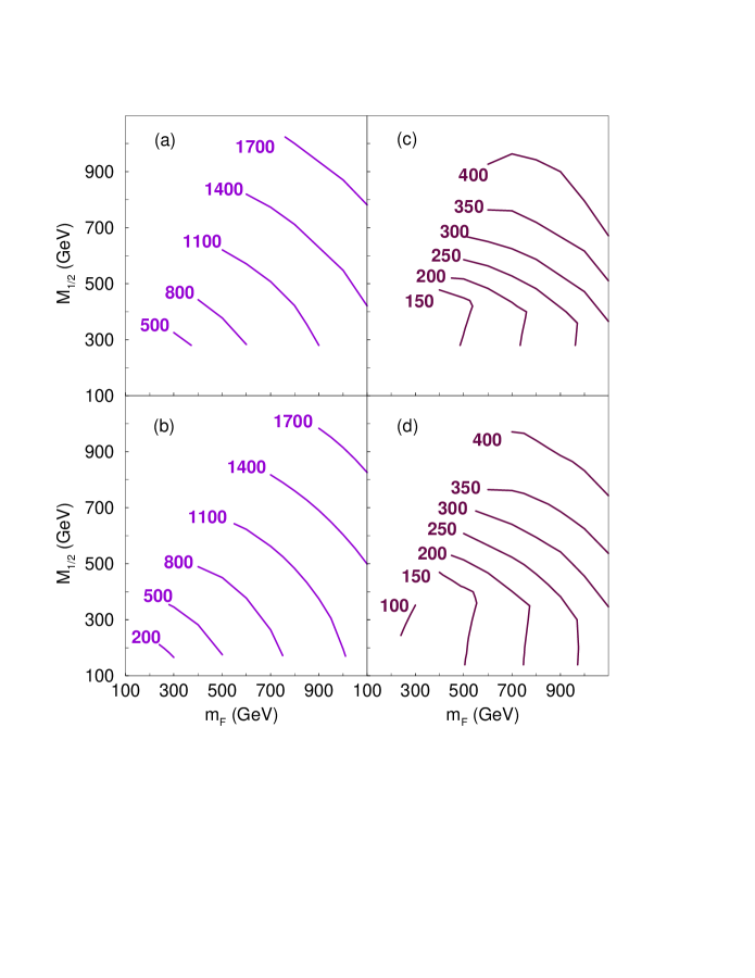
Figure 1: Contour lines of GUT scale parameters $m_{h}$ and $D$ determined by the condition of the radiative electroweak symmetry breaking, for two different values of $\mu$. (a) $m_{h}$, for $\mu=120$GeV.   (b) $m_{h}$, for $\mu=300$GeV.   (c) $D$, for $\mu=120$GeV.   (d) $D$, for $\mu=300$GeV.   Values in the plots are in GeV. In all plots $\tan\beta=50$, $A=0$, and $m_{F}=m_{F_{L}}=m_{F_{R}}$.

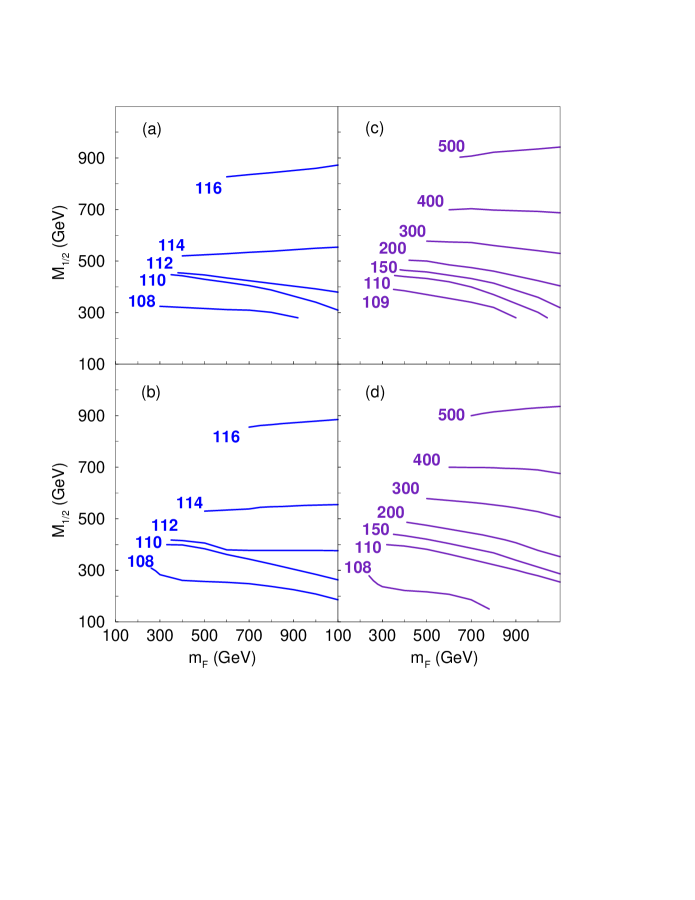
Figure 2: Contour lines of the light $CP$ even Higgs mass $m_{h^{0}}$ and pseudoscalar Higgs mass $m_{A^{0}}$, for two different values of $\mu$. (a) $m_{h^{0}}$, for $\mu=120$GeV.   (b) $m_{h^{0}}$, for $\mu=300$GeV.   (c) $m_{A^{0}}$, for $\mu=120$GeV.   (d) $m_{A^{0}}$, for $\mu=300$GeV.   Values in the plots are in GeV. In all plots $\tan\beta=50$, $A=0$, and $m_{F}=m_{F_{L}}=m_{F_{R}}$.

Figure 3: Contour lines of $\>\delta a_{\mu}({SUSY})\times 10^{10}$ and $\>BR$($\tau\to\mu+\gamma$ )$\times 10^{6}$, for two different values of $\mu$. (a) $\delta a_{\mu}({SUSY})\times 10^{10}$, for $\mu=120$GeV.   (b) $\delta a_{\mu}({SUSY})\times 10^{10}$, for $\mu=300$GeV.   (c) $BR$($\tau\to\mu+\gamma$ )$\times 10^{6}$, for $\mu=120$GeV.   (d) $BR$($\tau\to\mu+\gamma$ )$\times 10^{6}$, for $\mu=300$GeV.   In (a) and (b) the long-dashed curve marks the central value for $a_{\mu}$ not accounted for by the Standard Model, while the short-dashed curves mark the 2$\sigma$ limits of this quantity. The experimental upper limit on $\>BR$($\tau\to\mu+\gamma$ ) is $1.1\times 10^{6}$ [19]. In all plots $\tan\beta=50$, $A=0$, and $m_{F}=m_{F_{L}}=m_{F_{R}}$.

References

- [1] Muon g-2 Collaboration, H.N.Brown et al., hep-ex/0102017.
- [2] J. Lopez, D.V. Nanopoulos, and X. Wang, Phys. Rev. D49, 366 (1991); U. Chattopadhyay and P. Nath, Phys. Rev. D53, 1648 (1996); T. Moroi, Phys. Rev. D53, 6565 (1996); M. Carena, G.F. Giudice, and C.E.M. Wagner, Phys. Lett. B390, 234 (1997); T.Blažek, hep-ph/9912460.
-
[3]
L. Everett, G.L.Kane, S.Rigolin and L.Wang, hep-ph/0102145;
J.L.Feng and K.T.Matchev, hep-ph/0102146;
E.A.Baltz and P.Gondolo, hep-ph/0102147;
U.Chattopadhyay and P.Nath, hep-ph/0102157;
S.Komine, T.Moroi and M.Yamaguchi, hep-ph/0102204;
J.Hisano and K.Tobe, hep-ph/0102315;
J.Ellis, D.V.Nanopoulos and K.A.Olive, hep-ph/0102331;
R. Arnowitt, B. Dutta, B. Hu, and Y. Santoso, hep-ph/0102344. - [4] G.L.Kane, S.F.King and L.Wang, hep-ph/0010312.
- [5] S. F. King and Q. Shafi, Phys. Lett. B422, 135 (1998); T. Blažek, S. Raby, and K. Tobe, Phys. Rev. D62:055001 (2000).
- [6] S. F. King, M. Oliveira, Phys. Rev. D63:015010 (2001), hep-ph/0008183.
- [7] Y. Fukuda et al., Super-Kamiokande Collaboration, Phys. Lett. B433, 9 (1998); ibid. Phys. Lett. B436, 33 (1998); ibid. Phys. Rev. Lett. 81, 1562 (1998).
- [8] M. C. Gonzalez-Garcia and C. Peña-Garay, hep-ph/0009041.
- [9] S. F. King, Phys. Lett. B439, 350 (1998); S. F. King, Nucl. Phys. B562, 57 (1999); S. F. King, Nucl. Phys. B576, 85 (2000).
- [10] J. C. Pati, A. Salam, Phys. Rev. D10, 275 (1974).
- [11] I. Antoniadis and G. K. Leontaris, Phys. Lett. B216, 333 (1989); I. Antoniadis and G. K. Leontaris, and J. Rizos, Phys. Lett. B245, 161 (1990).
- [12] G. Shiu, S. H. H. Tye, Phys. Rev. D58, 106007 (1998).
-
[13]
S. F. King, Phys. Lett. B325, 129 (1994);
B. C. Allanach, S.F. King, Nucl. Phys. B456, 57 (1995);
B. C. Allanach, S. F. King, Nucl. Phys. B459, 75 (1996);
B. C. Allanach, S. F. King, G. K. Leontaris, S. Lola, Phys. Rev. D56, 2632 (1997); - [14] S.F.King and M.Oliveira, Phys. Rev. D63:095004 (2001), hep-ph/0009287.
- [15] T. Blažek, M. Carena, S. Raby and C.E.M. Wagner, Phys. Rev. D56, 6919 (1997).
- [16] M.Carena, J.R. Espinosa, M.Quiros and C. Wagner, Phys. Lett. B355, 209 (1995); M.Carena, M.Quiros and C. Wagner, Nucl. Phys. B461, 407 (1996); J.A. Casas, J.R. Espinosa, M. Quiros and A. Riotto, Nucl. Phys. B436, 3 (1995).
- [17] CDF coll., “Search for Neutral Supersymmetric Higgs Bosons in Collisions at TeV”, hep-ex/0010052.
- [18] R. Hempfling, Phys. Rev. D49, 6168 (1994). L. Hall, R. Ratazzi and U. Sarid, Phys. Rev. D50, 7048 (1994). M. Carena, M. Olechowski, S. Pokorski and C. Wagner, Nucl. Phys. B426, 269 (1994). T. Blažek, S. Raby, and S. Pokorski, Phys. Rev. D52, 4151 (1995).
- [19] J. Bartels et al. (Particle Data Group), Eur. Phys. J. C15, 1 (2000).