hep-ph/0105004

CERN–TH/2001-111

UMN–TH–2002/01, TPI–MINN–01/16

How Finely Tuned is Supersymmetric Dark Matter?

John Ellis¹ and Keith A. Olive^{1,2 1}TH Division, CERN, Geneva, Switzerland
²Theoretical Physics Institute, School of Physics and Astronomy,
University of Minnesota, Minneapolis, MN 55455, USA

Abstract

We introduce a quantification of the question in the title: the logarithmic sensitivity of the relic neutralino density $\Omega_{\chi}h^{2}$ to variations in input parameters such as the supersymmetric mass scales $m_{0},m_{1/2}$ and $A_{0}$, $\tan\beta$ and the top and bottom quark masses. In generic domains of the CMSSM parameter space with a relic density in the preferred range $0.1\leq\Omega_{\chi}h^{2}\leq 0.3$, the sensitivities to all these parameters are moderate, so an interesting amount of supersymetric dark matter is a natural and robust prediction. Within these domains, the accuracy in measuring the CMSSM and other input parameters at the LHC may enable the relic density to be predicted quite precisely. However, in the coannihilation regions, this might require more information on the supersymetric spectrum than the LHC is able to provide. There are also exceptional domains, such as those where direct-channel pole annihilation dominates, and in the ‘focus-point’ region, where the logarithmic sensitivity to the input parameters is greatly increased, and it would be more difficult to predict $\Omega_{\chi}h^{2}$ accurately.

CERN–TH/2001-111

May 2001

The annihilations of stable particles weighing $\mathrel{\hbox to0.0pt{\raise 2.15277pt\hbox{$<$}\hss}{\lower 2.15277pt\hbox{$\sim$}}}100$ TeV that were once in thermal equilibrium in the early Universe are able to produce a relic density comparable to the critical density. In particular, weakly-interacting stable particles weighing $\sim 1$ TeV may well have a cosmological density in the preferred range, if they were formerly in thermal equilibrium. An example is provided by the lightest supersymmetric particle, assumed to be the lightest neutralino $\chi$, which is expected to be stable in models with conserved $R$ parity [1]. For example, it is often remarked that supersymmetric dark matter ‘naturally’ has a relic density $\Omega_{\chi}h^{2}$ in the range $0.1\leq\Omega_{\chi}h^{2}\leq 0.3$ preferred by astrophysics and cosmology [2].

The TeV mass scale for supersymmetry is motivated independently by the hierarchy problem: how to make the small electroweak scale $m_{W}\ll m_{P}\sim 10^{19}$ GeV ‘natural’, without the need to fine-tune parameters at each order in perturbation theory [3]. This is possible if the supersymmetric partners of the Standard Model particles weigh $\mathrel{\hbox to0.0pt{\raise 2.15277pt\hbox{$<$}\hss}{\lower 2.15277pt\hbox{$\sim$}}}1$ TeV, but the amount of fine-tuning of supersymmetric parameters required to obtain the electroweak scale increases rapidly for sparticle masses $\gg 1$ TeV. In an attempt to quantify this, it was proposed [4, 5] to consider the logarithmic sensitivities of the electroweak scale to the supersymmetric model parameters $a_{i}$:

$$\Delta_{i}\equiv{a_{i}\over m_{W}}{\partial m_{W}\over\partial a_{i}}.$$ (1)

In the constrained MSSM (CMSSM) with universal soft supersymmetry-breaking parameters, the $a_{i}$ include the common scalar mass $m_{0}$, the common gaugino mass $m_{1/2}$, the common trilinear parameter $A_{0}$ at the GUT scale and the ratio of Higgs vev’s, $\tan\beta$, with the Higgs mixing parameter $\mu$ being determined (up to a sign) by the electroweak vacuum conditions. The measure (1) has been used, for example, to quantify the fine-tuning price imposed by the absence of sparticles at LEP [6]. The point has also been made that supersymmetric models with $0.1\leq\Omega_{\chi}h^{2}\leq 0.3$ tend to have small values of $\Delta\equiv{\rm Max}_{i}\Delta_{i}$ [7], establishing a link between (the absence of) hierarchical fine-tuning and good cosmology.

In this paper, we propose analogous measures of sensitivity to quantify the fine-tuning needed to obtain in the CMSSM a relic density $\Omega_{\chi}h^{2}$ in the range preferred by cosmology:

$$\Delta^{\Omega}_{i}\equiv{a_{i}\over\Omega_{\chi}}{\partial\Omega_{\chi}\over\partial a_{i}}.$$ (2)

The input parameters $a_{i}$ now include, along with the CMSSM parameters introduced above, the top- and bottom-quark masses, Standard Model parameters which are not so well known, and whose current uncertainties have important impacts on calculations of $\Omega_{\chi}h^{2}$. We also explore the accuracy to which measurements of the CMSSM parameters at the LHC might enable $\Omega_{\chi}h^{2}$ to be calculated [8].

In generic regions of the CMSSM parameter space, we find that the overall sensitivity

$$\Delta^{\Omega}\equiv\sqrt{\Sigma_{i}(\Delta^{\Omega}_{i})^{2}}$$ (3)

is relatively small: $\Delta^{\Omega}\mathrel{\hbox to0.0pt{\raise 2.15277pt\hbox{$<$}\hss}{\lower 2.15277pt\hbox{$\sim$}}}10$, implying that measurements of the input parameters at the 10 [1] % level will enable $\Omega_{\chi}h^{2}$ to be calculated to within a factor ${\cal O}(2)$ [${\cal O}(10\%)$]. The sensitivity $\Delta^{\Omega}$ is somewhat enhanced in the $\chi-{\tilde{\ell}}$ coannihilation region [9, 10], and here an accurate calculation of the relic density might not be possible with LHC measurements of the CMSSM parameters alone. There are also exceptional regions where the sensitivity of $\Delta^{\Omega}$ is greatly enhanced, notably at large $\tan\beta$ where there are ‘funnels’ in CMSSM parameter space due to rapid $\chi\chi\rightarrow H,A$ annihilation [11], and in the ‘focus-point’ region [12], where $\Delta^{\Omega}$ may rise to several hundred. In the focus-point region, there is extreme sensitivity to $m_{t}$: even if $m_{t}$ is measured at the 1 % level, $\Omega_{\chi}h^{2}$ may be uncertain by a large factor for any specific set of CMSSM parameters.

We start by outlining our procedure [11] for calculating the neutralino relic density $\Omega_{\chi}h^{2}$ and its sensitivity to the CMSSM parameters. As already mentioned, we consider as independent parameters the universal soft mass terms $m_{0},m_{1/2}$, the trilinear soft supersymmetry-breaking parameter $A_{0}$, and $\tan\beta$. We also assume unification of the gauge couplings at the GUT scale as an input into the renormalization-group calculations of the CMSSM parameters at the electroweak scale. The top- and bottom-quark masses are potentially important for the relic density calculations, particularly at large $\tan\beta$, and are relatively poorly known, so we also track the sensitivity of $\Omega_{\chi}h^{2}$ to their values. As defaults, we choose the running bottom-quark mass $m_{b}(m_{b})^{\overline{MS}}_{SM}=4.25$ GeV [13] and the top-quark pole mass $m_{t}=175$ GeV. However, for our calculations in the ‘focus-point’ region [12] we use $m_{t}=171$ GeV. This choice of $m_{t}$ allows us to display the focus-point region at values of $m_{0}$ between 1 and 2 TeV, for ease of comparison with [12]. If we had chosen $m_{t}=175$ GeV, our calculations would have located the focus-point region between 2 and 3 TeV.

More details of our code to evaluate $\Omega_{\chi}h^{2}$ are given in [11] and references therein, so here we note just a few relevant aspects. Calculations at small-to-moderate $\tan\beta\mathrel{\hbox to0.0pt{\raise 2.15277pt\hbox{$<$}\hss}{\lower 2.15277pt\hbox{$\sim$}}}25$ have no novel features, though we do recall the importance of including $\chi-{\tilde{\ell}}$ coannihilation processes at large $m_{1/2}$. As discussed in [11], several new coannihilation processes and diagrams become relevant at larger values of $\tan\beta$, which are included here. Also important at large $\tan\beta$ are direct-channel annihilation processes: $\chi\chi\rightarrow H,A$, where $H,A$ are the heavier neutral Higgs bosons in the CMSSM. Their treatment requires going beyond [14] the non-relativistic partial-wave expansion that is adequate elsewhere.

In order to calculate the sensitivities $\Delta^{\Omega}_{i}$ (2), we first define a grid in the $(m_{1/2},m_{0})$ plane for fixed $A_{0},\tan\beta,m_{t}$ and $m_{b}$, on which we compute the values of $\Omega_{\chi}h^{2}$. We then compute the differences in $\Omega_{\chi}h^{2}$ generated by small ($\mathrel{\hbox to0.0pt{\raise 2.15277pt\hbox{$<$}\hss}{\lower 2.15277pt\hbox{$\sim$}}}1$ %) changes in each of $m_{1/2},m_{0},A_{0},\tan\beta,m_{t}$ and $m_{b}$ individually. We then use these small finite differences to calculate the various sensitivities $\Delta^{\Omega}_{i}$ (2) and hence the overall sensitivity $\Delta^{\Omega}$ (3). Thus, obtaining our results is quite computation-intensive, with each of the $(m_{1/2},m_{0})$ planes that we show below requiring several times more CPU time than the calculations of $\Omega_{\chi}h^{2}$ shown previously [11]. For this reason, we have not increased the grid resolution sufficiently to clarify all the fluctuations (or small effects?) that we find in this analysis.

Fig. 1 displays the overall sensitivity $\Delta^{\Omega}$ (3) in the $(m_{1/2},m_{0})$ planes for four representative choices of the other CMSSM parameters. In each of these planes, the regions with relic density in the preferred range $0.1\leq\Omega_{\chi}h^{2}\leq 0.3$ are indicated by lighter shading, and the disallowed regions where the lightest supersymmetric particle is the ${\tilde{\tau}}_{1}$, rather than the lightest neutralino $\chi$, are shown by darker shading. In these figures, we show contours of constant values of the fine-tuning parmeter $\Delta^{\Omega}$. Contours of $\Delta^{\Omega}=3,30$, and 300 are shown by dashed (blue) curves of decreasing thickness. Contours of $\Delta^{\Omega}=10,100$, and 1000 are shown by solid (black) curves also of decreasing thickness. In Figure  1a, we show the two additional contours $\Delta^{\Omega}=1.5$ and 2, as dotted and dot-dashed curves respectively.

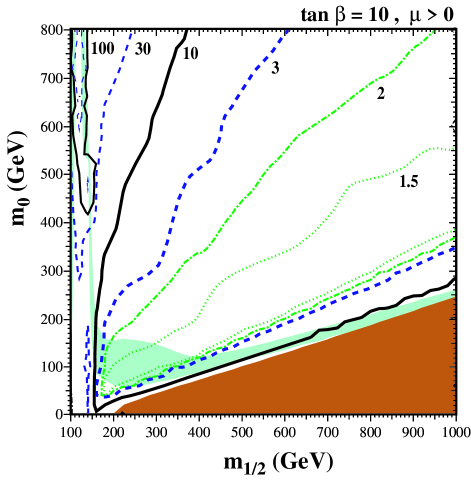
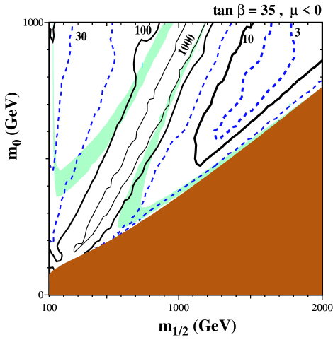
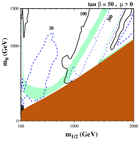
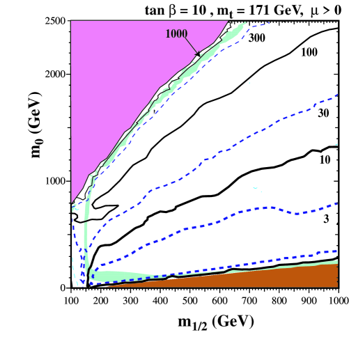
Figure 1: Contours of the total sensitivity $\Delta^{\Omega}$ in the $(m_{1/2},m_{0})$ planes for (a) $\tan\beta=10,\mu>0,m_{t}=175$ GeV, (b) $\tan\beta=35,\mu<0,m_{t}=175$ GeV, (c) $\tan\beta=50,\mu>0,m_{t}=175$ GeV, and (d) $\tan\beta=10,\mu>0,m_{t}=171$ GeV, all for $A_{0}=0$. The light (turquoise) shaded areas are the cosmologically preferred regions with $0.1\leq\Omega_{\chi}h^{2}\leq 0.3$. In the dark (brick red) shaded regions, the LSP is the charged ${\tilde{\tau}}_{1}$, so this region is excluded. In panel (d), the medium shaded (mauve) region is excluded by the electroweak vacuum conditions. The curves are contours of constant $\Delta^{\Omega}$, as described in the text.

Consider first panel (a), for $\tan\beta=10,A_{0}=0,\mu>0,m_{t}=175$ GeV and $m_{b}(m_{b})^{\overline{MS}}=4.25$ GeV. We see that, in a ‘generic’ domain of the $(m_{1/2},m_{0})$ plane for moderate values of $m_{0}/m_{1/2}$ in the approximate range 1/3 to 2, the overall sensitivity is also moderate: $\Delta^{\Omega}<10$. Indeed, there is a substantial domain of this $(m_{1/2},m_{0})$ plane where the sensitivity parameter $\Delta^{\Omega}<3$. Therefore, at least in this domain of parameter space, supersymmetric dark matter does not require fine tuning. We also note that the CMSSM value of $g_{\mu}-2$ is in good agreement [15] with the data [16] in this ‘generic’ domain at moderate $m_{0}/m_{1/2}$, as is the rate for $b\rightarrow s\gamma$ [17].

Moreover, the small magnitude of $\Delta^{\Omega}$ suggests that one might hope, with a % accuracy in the CMSSM parameters, to aim at a 10 % accuracy in calculating $\Omega_{\chi}h^{2}$. In this connection, we note that the preferred range $0.1\leq\Omega_{\chi}h^{2}\leq 0.3$ in this ‘generic’ domain requires moderate values $m_{1/2}\mathrel{\hbox to0.0pt{\raise 2.15277pt\hbox{$<$}\hss}{\lower 2.15277pt\hbox{$\sim$}}}400$ GeV and $m_{0}\mathrel{\hbox to0.0pt{\raise 2.15277pt\hbox{$<$}\hss}{\lower 2.15277pt\hbox{$\sim$}}}200$ GeV, where the LHC may be able to make detailed measurements of the sparticle spectrum and hence the CMSSM parameters [18]. We return later to a more careful consideration of the individual $\Delta^{\Omega}_{i}$ and the uncertainties in the corresponding $a_{i}$.

It is apparent in panel (a) of Fig. 1 that the overall sensitivity $\Delta^{\Omega}$ increases at both large and small values of $m_{0}/m_{1/2}$. The increase in $\Delta^{\Omega}$ at large $m_{0}/m_{1/2}$ is primarily due to the approach to the direct-channel $\chi\chi\rightarrow h$ pole. The enhanced annihilation cross section reduces the relic density to an acceptable level for finely tuned values of $m_{1/2}$, which is the reason $\Delta^{\Omega}$ takes on values in excess of 100 there. However, a close approach to this pole is forbidden by the LEP lower limits on the chargino mass $m_{\chi^{\pm}}$, and is also disfavoured by the LEP lower limit $m_{h}>113.5$ GeV [19], making this point somewhat moot.

The increase in $\Delta^{\Omega}$ close to a ray in the $(m_{1/2},m_{0})$ plane at small $m_{0}/m_{1/2}$ is due to the importance of coannihilation [9], whose significance varies with $m_{\tilde{\ell}}-m_{\chi}$ and hence the CMSSM parameters. However, we still find that $\Delta^{\Omega}<20$ in this coannihilation region, so the relic density does not require excessive fine-tuning in order to fall within the preferred range $0.1\leq\Omega_{\chi}h^{2}\leq 0.3$. On the other hand, the LHC may not be able to provide very detailed measurements of the sparticle spectrum in this region [20], so it may not facilitate a very accurate calculation of $\Omega_{\chi}h^{2}$. On the bright side, we note that this region does not agree well [15] with the value of $g_{\mu}-2$ reported recently [16].

We do not show $(m_{1/2},m_{0})$ planes for other low-to-moderate values of $\tan\beta\mathrel{\hbox to0.0pt{\raise 2.15277pt\hbox{$<$}\hss}{\lower 2.15277pt\hbox{$\sim$}}}25$, but simply remark that they are qualitatively similar to Fig. 1(a) for both signs of $\mu$. In particular, there are qualitatively similar zones where $\Delta^{\Omega}\mathrel{\hbox to0.0pt{\raise 2.15277pt\hbox{$<$}\hss}{\lower 2.15277pt\hbox{$\sim$}}}10$, or even $\mathrel{\hbox to0.0pt{\raise 2.15277pt\hbox{$<$}\hss}{\lower 2.15277pt\hbox{$\sim$}}}3$. These regions are also generally compatible with $g_{\mu}-2$ [16]. However, it should be remembered that the $b\rightarrow s\gamma$ constraint [17] (not shown here) excludes domains of small $m_{1/2}$ which increase as $\tan\beta$ increases, and are larger for $\mu<0$.

Panel (b) of Fig. 1 displays the $(m_{1/2},m_{0})$ plane for $\mu<0$ and $\tan\beta=35$, near the upper limit for which we find extensive regions of acceptable electroweak vacua for this sign of $\mu$ and our default choices of $m_{t}$ and $m_{b}$ [11]. We note that the sensitivity $\Delta^{\Omega}$ is generally higher than in panel (a) for $\tan\beta=10$, foreshadowing the breakdown of the electroweak vacuum conditions. We also see a ‘funnel’ at $m_{0}\sim m_{1/2}$, where the relic density varies rapidly, reflecting the importance of direct-channel $\chi\chi\rightarrow H,A$ pole annihilations, so that $\Delta^{\Omega}$ is large. Indeed, $\Delta^{\Omega}\sim 100$ in the cosmological funnel, and even exceeds 1000 deep in the pole region where the relic density is very small. The sensitivity measure $\Delta^{\Omega}$ is significantly larger than for $\tan\beta=10$ also at larger values of $m_{0}/m_{1/2}\sim 2$, reflecting the fact that the preferred range of $m_{0}$ increases relatively rapidly as $\tan\beta$ increases and the rapid-annihilation ‘funnel’ moves to higher $m_{0}\sim m_{1/2}$. The behaviour of $\Delta^{\Omega}$ in the coannihilation region of Fig. 1(b) is qualitatively similar to that in Fig. 1(a), whilst being somewhat more elevated. In the good cosmological region with low $m_{1/2}$, $\Delta^{\Omega}\mathrel{\raise 1.29167pt\hbox{$>$\kern-7.5pt\lower 4.30554pt\hbox{$\sim$}}}20$.

Panel (c) of Fig. 1 displays the case $\mu>0$ and $\tan\beta=50$, which is again close to the upper limit for which we find extensive regions of acceptable electroweak vacua for this sign of $\mu$ and our default choices of $m_{t}$ and $m_{b}$ [11]. Panel (c) has many qualitative features in common with panel (b), notably the very elevated values of $\Delta^{\Omega}$ around a rapid-annihilation ‘funnel’, and the somewhat elevated values of $\Delta^{\Omega}$ in the regions at higher and lower values of $m_{0}/m_{1/2}$.

Finally, panel (d) of Fig. 1 displays another case with $\mu>0$ and $\tan\beta=10$, this time for $m_{t}=171$ GeV. Its features are rather similar to those of panel (a) for $m_{0}\mathrel{\hbox to0.0pt{\raise 2.15277pt\hbox{$<$}\hss}{\lower 2.15277pt\hbox{$\sim$}}}800$ GeV, but now we also see the ‘focus-point’ region of acceptable $\Omega_{\chi}h^{2}$ for $m_{0}\mathrel{\hbox to0.0pt{\raise 2.15277pt\hbox{$>$}\hss}{\lower 2.15277pt\hbox{$\sim$}}}1000$ GeV . The ‘focus-point’ region adjoins the (mauve) shaded region where we do not find a consistent electroweak vacuum. The fact that the ‘focus-point’ region moves rapidly with a small change in $m_{t}$ largely explains the high values of the sensitivity parameter $\Delta^{\Omega}\sim 500$ in this region: analogous high sensitivity to $m_{t}$ can be seen in Fig. 9 of the second paper in [12] .

As an aid to better understanding of the origins of the variations in the overall sensitivity measure $\Delta^{\Omega}$ in Fig. 1, we display in Fig. 2 the values of all the individual $\Delta^{\Omega}_{i}$ along various illustrative slices through the CMSSM parameter space at constant $m_{0}$ or $m_{1/2}$. The vertical (pink) shaded strips in the panels of Fig. 2 show the regions where the relic density falls within the preferred range $0.1\leq\Omega_{\chi}h^{2}\leq 0.3$.

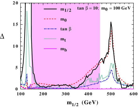
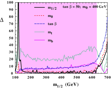
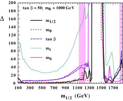
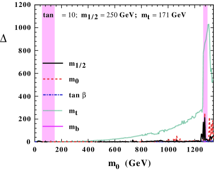
Figure 2: Fine-tuning sensitivities along illustrative slices through the CMSSM parameter space: for (a) $m_{0}=100$ GeV when $\tan\beta=10,\mu>0,m_{t}=175$ GeV, (b) $m_{0}=400$ GeV when $\tan\beta=50,\mu>0,m_{t}=175$ GeV, (c) $m_{0}=1000$ GeV when $\tan\beta=50,\mu>0,m_{t}=175$ GeV, and (d) for $m_{1/2}=250$ GeV when $\tan\beta=10,\mu>0,m_{t}=171$ GeV, all for $A_{0}=0$. The sensitivities $\Delta^{\Omega}_{i}$ to different input parameters are plotted using different line styles, as indicated. The sensitivity to $A_{0}$ is always negligible, and is not shown. The vertical (pink) shaded bands have $0.1\leq\Omega_{\chi}h^{2}\leq 0.3$.

Panel (a) of Fig. 2 is for $m_{0}=100$ GeV when $\tan\beta=10,\mu>0,A_{0}=0,m_{t}=175$ GeV and $m_{b}(m_{b})^{\overline{MS}}=4.25$ GeV, corresponding to a slice of Fig. 1(a). Looking first at the ‘generic’ region where $150$ GeV $\mathrel{\hbox to0.0pt{\raise 2.15277pt\hbox{$<$}\hss}{\lower 2.15277pt\hbox{$\sim$}}}m_{1/2}\mathrel{\hbox to0.0pt{\raise 2.15277pt\hbox{$<$}\hss}{\lower 2.15277pt\hbox{$\sim$}}}400$ GeV, we see that the dominant sensitivities $\Delta^{\Omega}_{i}$ are those to $m_{0}$ and $m_{1/2}$, both of which are close to unity. Next in importance is the sensitivity to $m_{t}$, which is ${\cal O}(1/2)$. Finally, the sensitivities to $\tan\beta,m_{b}(m_{b})^{\overline{MS}}$ and particularly $A_{0}$ are rather negligible in this domain. Clearly visible is a sharp increase in some of the $\Delta^{\Omega}_{i}$ for $m_{1/2}\mathrel{\hbox to0.0pt{\raise 2.15277pt\hbox{$<$}\hss}{\lower 2.15277pt\hbox{$\sim$}}}150$ GeV, dominated by jumps in the sensitivity to $m_{1/2}$ and $m_{t}$ as $m_{\chi}$ traverses the value $m_{h}/2$, and the rate of $\chi\chi\rightarrow h$ annihilation changes rapidly. However, as already mentioned, this pole region is not relevant to the dark matter issue, because it is excluded by the LEP constraint on $m_{\chi^{\pm}}$ and would, in any case, give a very suppressed relic density $\Omega_{\chi}h^{2}\ll 0.1$ in all but a very narrow strip in $m_{1/2}$. Also visible for $m_{1/2}\mathrel{\hbox to0.0pt{\raise 2.15277pt\hbox{$>$}\hss}{\lower 2.15277pt\hbox{$\sim$}}}400$ GeV are more gradual rises in some of the $\Delta^{\Omega}_{i}$ as $m_{\chi}-m_{\tilde{\tau}_{1}}\rightarrow 0^{-}$ in the coannihilation region [9], followed by falls in the disallowed domain where $m_{\chi}>m_{\tilde{\tau}_{1}}$. The sensitivities to $m_{0}$ and $m_{1/2}$ are the largest, and are very similar, as is to be expected because they are the key parameters controlling $m_{\chi}-m_{\tilde{\tau}_{1}}$. This behavior is easily understood when one takes into account the exponential sensitivity of coannihilation to $m_{\chi}-m_{\tilde{\tau}_{1}}$ and recongizes the strong dependence of $m_{\tilde{\tau}_{1}}$ on both $m_{1/2}$ and $m_{0}$ and $m_{\chi}$ on $m_{1/2}$. The sensitivity to $m_{t}$ arises from the renormalization-group equations used to determine the low-energy parameters in terms of the GUT-scale input parameters, and $\tan\beta$ also enters in the determination of the $m_{\chi}-m_{\tilde{\tau}_{1}}=0$ contour. We see that, even in this region, none of the individual $\Delta^{\Omega}_{i}$ exceeds 15, and recall that, as seen in Fig. 1(a), the combined $\Delta^{\Omega}\mathrel{\hbox to0.0pt{\raise 2.15277pt\hbox{$<$}\hss}{\lower 2.15277pt\hbox{$\sim$}}}20$ in the region of preferred relic density $0.1\leq\Omega_{\chi}h^{2}\leq 0.3$ for $\tan\beta=10$.

Panel (b) of Fig. 2 shows a slice at fixed $m_{0}=400$ GeV through Fig. 1(c), for $\tan\beta=50,\mu>0,A_{0}=0,m_{t}=175$ GeV and $m_{b}(m_{b})^{\overline{MS}}=4.25$ GeV. In the generic region where $m_{1/2}\mathrel{\hbox to0.0pt{\raise 2.15277pt\hbox{$<$}\hss}{\lower 2.15277pt\hbox{$\sim$}}}600$ GeV, which includes the range where $0.1\leq\Omega_{\chi}h^{2}\leq 0.3$, we see that the dominant sensitivity (between 20 and 30) is that to $m_{t}$, which is associated with the ‘squeezing’ of this region as the ‘funnel’ moves towards the vertical axis. Next in importance for $m_{1/2}\mathrel{\hbox to0.0pt{\raise 2.15277pt\hbox{$<$}\hss}{\lower 2.15277pt\hbox{$\sim$}}}600$ GeV are the sensitivities ($\mathrel{\hbox to0.0pt{\raise 2.15277pt\hbox{$<$}\hss}{\lower 2.15277pt\hbox{$\sim$}}}10$) to $\tan\beta$ and $m_{b}(m_{b})^{\overline{MS}}=4.25$ GeV, which also originate from their effects on the ‘funnel’. The sensitivities to $m_{0}$ and $m_{1/2}$ are much smaller, even comparable to those in panel (a), and the sensitivity to $A_{0}$ is negligible, as always for $A_{0}=0$. The region of high sensitivity when $m_{1/2}\mathrel{\hbox to0.0pt{\raise 2.15277pt\hbox{$<$}\hss}{\lower 2.15277pt\hbox{$\sim$}}}150$ GeV is actually excluded by the $b\rightarrow s\gamma$ constraint, which imposes $m_{1/2}\mathrel{\hbox to0.0pt{\raise 2.15277pt\hbox{$>$}\hss}{\lower 2.15277pt\hbox{$\sim$}}}300$ GeV for this value of $m_{0}$ and the other parameters.

Panel (c) of Fig. 2 shows a slice at fixed $m_{0}=1000$ GeV, again through Fig. 1(c), for $\tan\beta=50,\mu>0,A_{0}=0,m_{t}=175$ GeV and $m_{b}(m_{b})^{\overline{MS}}=4.25$ GeV. As also seen in Fig. 1(c), there are much narrower ranges of $m_{1/2}$ where $0.1\leq\Omega_{\chi}h^{2}\leq 0.3$: one on the left side of the rapid annihilation ‘funnel’, a much narrower region on the right side when $m_{1/2}\sim 1600$ GeV, that is not shown in Fig. 2(c), and another narrow region in the coannihilation region when $m_{1/2}\sim 1800$ GeV. The dominant sensitivity to the left of the ‘funnel’ is that to $m_{t}$, followed by those to $\tan\beta$ and $m_{b}$. These all increase as the ‘funnel’ is approached, reflecting its sensitivities to these parameters. In the coannihilation region of Fig. 2(c), the sensitivities to $\tan\beta,m_{0}$ and $m_{1/2}$ dominate as $m_{\tilde{\tau}_{1}}-m_{\chi}\rightarrow 0^{+}$, and are all more important than for $\tan\beta=10$, as shown in Fig. 2(a).

Finally, panel (d) of Fig. 2 shows a slice at fixed $m_{1/2}=250$ GeV through Fig. 1(d), for $\tan\beta=10,\mu>0,A_{0}=0,m_{t}=171$ GeV and $m_{b}(m_{b})^{\overline{MS}}=4.25$ GeV. This cuts through both the ‘focus-point’ region and the ‘generic’ domain, for which a different slice was shown in panel (a). The most noticeable feature is a strong growth in the sensitivity to $m_{t}$ as the ‘focus-point’ region is approached, with a maximum value $\Delta^{\Omega}_{m_{t}}\simeq 1000$: see also Fig. 9 of the second paper in [12]. We also note increased sensitivities to $m_{1/2}$ and $m_{0}$ in this region: $\Delta^{\Omega}_{m_{1/2},m_{0}}\simeq 200$, reflecting the narrowness of the ‘focus-point’ strip in the $(m_{1/2},m_{0})$ plane. The sensitivities in the ‘generic’ domain at smaller $m_{1/2}$ are invisible in this plot, but are very similar to those shown in Fig. 2(a), namely $\Delta^{\Omega}_{i}\mathrel{\hbox to0.0pt{\raise 2.15277pt\hbox{$<$}\hss}{\lower 2.15277pt\hbox{$\sim$}}}{\cal O}(1)$.

Finally, we consider what light this analysis casts on the accuracy with which LHC measurements might eventually enable $\Omega_{\chi}h^{2}$ to be calculated [8]. We assume that $\delta m_{t}/m_{t}=1\%$ in the LHC era, and that $\delta m_{b}/m_{b}=5\%$ [13] in all cases. Detailed studies of the precision with which a combination of LHC measurements could constrain CMSSM parameters have been made for a limited number of benchmark points [18, 21, 22, 23]. Unfortunately, these LHC benchmark points are now outdated, e.g., because the relic density is too high or because $m_{h}$ is too low, and they are often bad also for $g_{\mu}-2$ and/or $b\rightarrow s\gamma$. However, we select for our analysis two LHC points that yield $\Omega_{\chi}h^{2}<0.3$, and attempt to extract from them useful indicators for points that yield $\Omega_{\chi}h^{2}$ in the preferred range.

LHC Point 5: This is the LHC point for which the most detailed studies are available [18, 21, 22]. It has $\mu>0$ and the following values of the CMSSM parameters :

$$m_{0}=100~{}{\rm GeV},\;m_{1/2}=300~{}{\rm GeV},\;\tan\beta=2$$ (4)

corresponding, according to our calculations, to $\Omega_{\chi}h^{2}=0.22$ (within the preferred range) and $m_{h}\simeq 91$ GeV [24] (which is excluded by LEP). Moreover, though its value of $b\rightarrow s\gamma$ is satisfactory, its value of $g_{\mu}-2$ is too small. However, it may serve as a useful indicator. At this point, a number of spectroscopic measurements would have been possible at the LHC [18, 21, 22], and the errors in the LHC determinations of the numerical parameters were estimated to be:

$$\delta m_{0}=3.6~{}{\rm GeV},\;\delta m_{1/2}=5.0~{}{\rm GeV},\;\delta\tan\beta=0.18.$$ (5)

Extending our analysis of the $\Delta^{\Omega}_{i}$ to this specific extra case, we find the following sensitivities to parameters:

$$\Delta^{\Omega}_{m_{0}}=0.80,\;\Delta^{\Omega}_{m_{1/2}}=0.92,\;\Delta^{\Omega}_{\tan\beta}=0.07,\;\Delta^{\Omega}_{m_{t}}\simeq\Delta^{\Omega}_{m_{b}}\simeq 0.$$ (6)

Combining in quadrature the errors in (5) with the sensitivities (6) in the calculation of $\Omega_{\chi}h^{2}$, we estimate

$${\delta\Omega_{\chi}h^{2}\over\Omega_{\chi}h^{2}}\;\mathrel{\hbox to0.0pt{\raise 2.15277pt\hbox{$>$}\hss}{\lower 2.15277pt\hbox{$\sim$}}}\;{1\over 30};$$ (7)

where the inequality sign recalls that there are certainly other errors in the calculation of $\Omega_{\chi}h^{2}$, that may not be negligible. However, we infer from (7) that an accurate calculation of $\Omega_{\chi}h^{2}$ may be possible in ‘generic’ domains of the allowed CMSSM parameter space for moderate $\tan\beta$.

LHC Point 6: This [23] is the only LHC point with large $\tan\beta$. It has $\mu>0$ and the following values of the CMSSM parameters:

$$m_{0}=200~{}{\rm GeV},\;m_{1/2}=200~{}{\rm GeV},\;\tan\beta=45$$ (8)

corresponding, according to our calculations, to $\Omega_{\chi}h^{2}=0.045$ (below our preferred range, but not excluded) and $m_{h}=112$ GeV (which may be allowed by LEP when one allows for theoretical uncertainties). However, neither $b\rightarrow s\gamma$ nor $g_{\mu}-2$ are satisfactory for this point. The errors in the LHC determinations of the CMSSM parameters were estimated to be:

$$\delta m_{0}=29~{}{\rm GeV},\;\delta m_{1/2}=9~{}{\rm GeV},\;\delta\tan\beta=5.$$ (9)

In this case, we find that the parameter sensitivities are somehwat more elevated:

$$\Delta^{\Omega}_{m_{0}}=2.45,\;\Delta^{\Omega}_{m_{1/2}}=1.65,\;\Delta^{\Omega}_{\tan\beta}=-5.18,\;\Delta^{\Omega}_{m_{t}}=9.0,\;\Delta^{\Omega}_{m_{b}}=-3.51,$$ (10)

in view of which we conclude that

$${\delta\Omega_{\chi}h^{2}\over\Omega_{\chi}h^{2}}\;=\;{\cal O}(1)$$ (11)

in this case.

We note, moreover, that, for this value of $\tan\beta$, $\Omega_{\chi}h^{2}$ is large enough to be in the range preferred by cosmology only if larger values of $m_{0}$ and/or $m_{1/2}\mathrel{\hbox to0.0pt{\raise 2.15277pt\hbox{$>$}\hss}{\lower 2.15277pt\hbox{$\sim$}}}400$ GeV are chosen. We recall that LHC Points 1 and 2 had $m_{0}=m_{1/2}=400$ GeV [18], and that in these cases the limited LHC measurements did not provide any accuracy in the determination of $m_{0}$. (These points also had $\Omega_{\chi}h^{2}\mathrel{\hbox to0.0pt{\raise 2.15277pt\hbox{$>$}\hss}{\lower 2.15277pt\hbox{$\sim$}}}1.6$, acceptable $b\rightarrow s\gamma$ and unacceptable $g_{\mu}-2$.) We conclude from this discussion and (11) that an accurate calculation of $\Omega_{\chi}h^{2}$ may not be possible at large $\tan\beta$ using LHC data alone.

For the record, we recall that LHC Point 3 [18] had $m_{0}=200~{}{\rm GeV},m_{1/2}=100~{}{\rm GeV}$, $\tan\beta=2$ and $\mu<0$, leading to $m_{h}\sim 67$ GeV [24], which is far too small. This points also had $\Omega_{\chi}h^{2}\simeq 0.38$ (rather too high) and unacceptable $g_{\mu}-2$, though $b\rightarrow s\gamma$ was satisfactory. We do not discuss this point in detail, but note that, like at Point 5, $\Omega_{\chi}h^{2}$ could in principle be calculated quite accurately using LHC data. Finally, LHC Point 4 has $m_{0}=800~{}{\rm GeV},m_{1/2}=200~{}{\rm GeV},\tan\beta=10$, leading to $\Omega_{\chi}h^{2}=5.6$, rendering it uninteresting for this analysis. For completeness, we note that this point had $m_{h}\simeq 111$ GeV, acceptable $b\rightarrow s\gamma$ and unacceptable $g_{\mu}-2$. We also note that, although some sparticle measurements are possible in the coannihilation region [20], it seems unlikely that LHC measurements alone will constrain the CMSSM parameters sufficiently to enable $\Omega_{\chi}h^{2}$ to be calculated accurately.

To conclude: We have demonstrated in this paper that there are ‘generic’ domains of CMSSM parameter space at moderate $\tan\beta$ where the sensitivity $\Delta^{\Omega}$ of the relic density $\Omega_{\chi}h^{2}$ is rather small. Thus, obtaining $\Omega_{\chi}h^{2}$ in the range preferred by astrophysics and cosmology does not require ‘fine-tuning’ of the values of the CMSSM parameters. The sensitivity of $\Omega_{\chi}h^{2}$ to the CMSSM parameters is somewhat increased in the coannihilation region [9], but not to an alarming extent. It is also increased at large $\tan\beta$, particularly in the ‘funnel’ regions where rapid $\chi\chi\rightarrow H,A$ annihilations are important [11]. We also found large values of $\Delta^{\Omega}$ in the ‘focus-point’ region [12], where the CMSSM parameters and particularly $m_{t}$ must be adjusted for a given set of supersymmetric input parameters, if $\Omega_{\chi}h^{2}$ is to fall within the preferred range. The tracking of the individual sensitivities, $\Delta^{\Omega}_{i}$ clarifies which parameters must be measured and treated carefully in order to calculate $\Omega h^{2}$ reliably.

In the generic regions with low $\Delta^{\Omega}$, LHC measurements [18] may enable $\Omega_{\chi}h^{2}$ to be calculated accurately. It would be interesting to study how accurately the CMSSM parameters could be measured at a new set of benchmark points that respect the constraints imposed by LEP and other recent experiments [25], both at the LHC and with a possible linear $e^{+}e^{-}$ collider. As already mentioned, there are clearly cases where the LHC alone cannot determine the CMSSM parameters with sufficient precision to enable $\Omega_{\chi}h^{2}$ to be calculated accurately, and it would be interesting to see how a linear $e^{+}e^{-}$ collider could contribute. A successful, accurate calculation of $\Omega_{\chi}h^{2}$ on the basis of accelerator data would surely be the culmination of supersymmetric dark matter studies, making this a worthwhile objective to pursue.

Acknowledgments
The work of K.A.O. was partially supported by DOE grant DE–FG02–94ER–40823.

References

- [1] P. Fayet, Unification of the Fundamental Particle Interactions, eds. S. Ferrara, J. Ellis and P. van Nieuwenhuizen (Plenum, New York, 1980), p.587.
- [2] J. Ellis, J.S. Hagelin, D.V. Nanopoulos, K.A. Olive and M. Srednicki, Nucl. Phys. B238 (1984) 453; see also H. Goldberg, Phys. Rev. Lett. 50 (1983) 1419.
- [3] L. Maiani, Proceedings of the 1979 Gif-sur-Yvette Summer School On Particle Physics, 1; G. ’t Hooft, in Recent Developments in Gauge Theories, Proceedings of the Nato Advanced Study Institute, Cargese, 1979, eds. G. ’t Hooft et al., (Plenum Press, NY, 1980); E. Witten, Phys. Lett. B105 (1981) 267.
- [4] J. Ellis, K. Enqvist, D. V. Nanopoulos and F. Zwirner, Mod. Phys. Lett. A1 (1986) 57.
- [5] R. Barbieri and G. F. Giudice, Nucl. Phys. B306 (1988) 63.
- [6] P. H. Chankowski, J. Ellis and S. Pokorski, Phys. Lett. B423 (1998) 327; P. H. Chankowski, J. Ellis, M. Olechowski and S. Pokorski, Nucl. Phys. B544 (1999) 39.
- [7] P. H. Chankowski, J. Ellis, K. A. Olive and S. Pokorski, Phys. Lett. B452 (1999) 28.
- [8] M. Drees, Y. G. Kim, M. M. Nojiri, D. Toya, K. Hasuko and T. Kobayashi, Phys. Rev. D63 (2001) 035008.
- [9] J. Ellis, T. Falk and K. A. Olive, Phys. Lett. B444, 367 (1998); J. Ellis, T. Falk, K. A. Olive and M. Srednicki, Astropart. Phys. 13 (2000) 181.
- [10] M. E. Gómez, G. Lazarides and C. Pallis, Phys. Rev. D61, 123512 (2000) and Phys. Lett. B487, 313 (2000); R. Arnowitt, B. Dutta and Y. Santoso, hep-ph/0102181.
- [11] J. Ellis, T. Falk, G. Ganis, K. A. Olive and M. Srednicki, hep-ph/0102098.
- [12] J. L. Feng, K. T. Matchev and T. Moroi, Phys. Rev. Lett. 84 (2000) 2322 and Phys. Rev. D 61 (2000) 075005; J. L. Feng, K. T. Matchev and F. Wilczek, Phys. Lett. B482 (2000) 388 and Phys. Rev. D63 (2001) 045024.
- [13] Compare D.E. Groom et al., Euro. Phys. J. C15 (2000) 1, http://pdg.lbl.gov/.
- [14] K. Griest and D. Seckel, Phys. Rev. D43 (1991) 3191; P. Gondolo and G. Gelmini, Nucl. Phys. B360 (1991) 145.
- [15] J. Ellis, D. V. Nanopoulos and K. A. Olive, hep-ph/0102331; for other recent papers on the CMSSM interpretation of , see L. Everett, G. L. Kane, S. Rigolin and L. Wang, hep-ph/0102145; J. L. Feng and K. T. Matchev, hep-ph/0102146; E. A. Baltz and P. Gondolo, hep-ph/0102147; U. Chattopadhyay and P. Nath, hep-ph/0102157; S. Komine, T. Moroi and M. Yamaguchi, hep-ph/0102204; J. Hisano and K. Tobe, hep-ph/0102315. R. Arnowitt, B. Dutta, B. Hu and Y. Santoso, hep-ph/0102344; K. Choi, K. Hwang, S. K. Kang, K. Y. Lee and W. Y. Song, hep-ph/0103048; S. P. Martin and J. D. Wells, hep-ph/0103067; S. Komine, T. Moroi and M. Yamaguchi, hep-ph/0103182; H. Baer, C. Balazs, J. Ferrandis and X. Tata, hep-ph/0103280.
- [16] H. N. Brown et al., Muon Collaboration, Phys. Rev. Lett. 86 (2001) 2227.
- [17] CLEO Collaboration, M.S. Alam et al., Phys. Rev. Lett. 74 (1995) 2885 as updated in S. Ahmed et al., CLEO CONF 99-10; K. Abe et al., Belle Collaboration, hep-ex/0103042; C. Degrassi, P. Gambino and G. F. Giudice, JHEP 0012 (2000) 009; see also M. Carena, D. Garcia, U. Nierste and C. E. Wagner, hep-ph/0010003.
- [18] I. Hinchliffe, F. E. Paige, M. D. Shapiro, J. Soderqvist and W. Yao, Phys. Rev. D55 (1997) 5520; ATLAS Collaboration, Detector and Physics Performance Technical Design Report, http://atlasinfo.cern.ch/Atlas/GROUPS/PHYSICS/TDR/access.html.
-
[19]
ALEPH collaboration, R. Barate et al., Phys. Lett. B495
(2000) 1;
L3 collaboration, M. Acciarri et al., Phys. Lett. B495 (2000) 18;
DELPHI collaboration, P. Abreu et al., Phys. Lett. B 499 (2001) 23;
OPAL collaboration, G. Abbiendi et al., Phys. Lett. B499 (2001) 38.
For a preliminary compilation of the LEP data presented on Nov. 3rd, 2000, see:
P. Igo-Kemenes, for the LEP Higgs working group,
http://lephiggs.web.cern.ch/LEPHIGGS/talks/index.html. - [20] S. Abdullin and F. Charles, Nucl. Phys. B547 (1999) 60.
- [21] G. Polesello, L. Poggioli, E. Richter-Wa̧s and J. Söderqvist, ATLAS Internal Note PHYS-No-111 (1997).
- [22] H. Bachacou, I. Hinchliffe and F. E. Paige, Phys. Rev. B62 (2000) 015009.
- [23] I. Hinchliffe and F. E. Paige, Phys. Rev. D61 (2000) 095011.
- [24] For our numerical analysis, here we use the results of M. Carena, H. E. Haber, S. Heinemeyer, W. Hollik, C. E. Wagner and G. Weiglein, Nucl. Phys. B580 (2000) 29.
- [25] A proposal for new post-LEP benchmarks is now being prepared by M. Battaglia, A. de Roeck, F. Gianotti, K. Matchev, L. Pape, G. Wilson and the present authors.