Density Fluctuations and Primordial Black Hole Formation in Natural Double Inflation in Supergravity

Abstract

We investigate the recently proposed natural double inflation model in supergravity. Chaotic inflation first takes place by virtue of the Nambu-Goldstone-like shift symmetry. During chaotic inflation, an initial value of second inflation (new inflation) is set, which is adequately far from the local maximum of the potential due to the small linear term in the Kähler potential. Then, primordial fluctuations within the present horizon scale may be produced during both inflations. Primordial fluctuations responsible for anisotropies of the cosmic microwave background radiation and the large scale structure are produced during chaotic inflation, while fluctuations on smaller scales are produced during new inflation. Because of the peculiar nature of new inflation, they can become as large as $10^{-1}$-$10^{-2}$, which may lead to the formation of primordial black holes.

I Introduction

Inflation is the most attractive mechanism to generate primordial density fluctuations responsible for anisotropies of the cosmic microwave background radiation (CMB) and the large scale structure, in addition to solving the flatness and the horizon problem [2]. Realistic inflation models should be constructed in the context of the supersymmetric theory, especially, its local version, supergravity (SUGRA) [3] because supersymmetry (SUSY) guarantees the flatness of the inflaton against radiative corrections and gives a natural solution to the hierarchy problem between the inflationary scale and the electroweak scale [4].

New inflation [5] is very attractive in the context of SUGRA because it takes place at a low energy scale and naturally leads to a sufficiently low reheating temperature to avoid the overproduction of gravitinos. However, roughly speaking, new inflation has two severe problems [2]. One is the initial value problem: that is, the inflaton must be fine-tuned near the local maximum of the potential for sufficient inflation. The other is the flatness (longevity) problem: that is, why the universe lives so long beyond the Planck time. Asaka, Kawasaki, and the present author [6] found that, due to gravitationally suppressed interactions with particles in the thermal bath, the inflaton can dynamically go to the local maximum of its potential. However, the other problem still exists unless the universe is open at the beginning. Izawa, Kawasaki, and Yanagida [7] considered another type of inflation (called preinflation) which takes place before new inflation and drives the inflaton for new inflation dynamically toward the local maximum of its potential. If preinflation is chaotic inflation [8], the longevity problem is solved too.

It, however, is believed to be difficult to realize chaotic inflation in SUGRA. This is mainly because a scalar potential in minimal SUGRA has an exponential factor with the form $\exp(|\phi|^{2}/M_{G}^{2})$ so that any scalar field $\phi$ cannot take a value much larger than the reduced Planck scale $M_{G}\simeq 2.4\times 10^{18}$ GeV. Several supergravity chaotic inflation models were proposed by use of functional degrees of freedom of the Kähler potential in SUGRA [9, 10]. But, there are no symmetry reasons to have such proposed forms. Recently, Kawasaki, Yanagida, and the present author [11] proposed a natural model of chaotic inflation in SUGRA by use of the Nambu-Goldstone-like shift symmetry. Motivated by this model, Yokoyama and the present author [12] considered chaotic inflation followed by new inflation, where chaotic inflation first takes place around the Planck scale to solve the longevity problem and gives an adequate initial condition for new inflation. Thus double inflation has been proposed as a solution of initial condition problems of some types of inflation [7, 14]. (See Refs. [13, 14] for the initial value problem and its solution of hybrid inflation.)

On the other hand, double inflation is also motivated by observational results. One motivation is to reconcile predicted spectra with observations of the large scale structure [15]. It is known that a standard cold dark matter (CDM) model in a flat universe with a nearly scale-invariant spectrum cannot reproduce the observation of the large scale structure. Furthermore, the recent observations of anisotropies of the CMB by the BOOMERANG experiment [16] and MAXIMA experiment [17] found a relatively low second acoustic peak. Another motivation is to produce primordial black holes (PBHs) [18, 19, 20]. Massive compact halo objects (MACHOs) are observed through gravitational microlensing effects [21], which are a possible candidate of dark matter. Furthermore, PBHs evaporating now may be a source of antiproton flux observed by the BESS experiment [22] or responsible for short gamma ray bursts (GRBs) [23]. Though many double inflations have been considered, they are often discussed in a simple toy model with two massive scalar fields. However, a natural double inflation model in SUGRA is recently proposed [24], where there are no initial condition problems and the model parameters are natural in the ’t Hooft sense [25]. In this model, chaotic inflation takes place first of all, during which an initial value of new inflation is dynamically set due to the supergravity effects. It can be adequately far from the local maximum of the potential due to the small linear term of the inflaton in the Kähler potential. Therefore primordial density fluctuations responsible for the observable universe can be attributed to both inflations, that is, chaotic inflation produces primordial fluctuations on large cosmological scales and new inflation on smaller scales. The energy scale of new inflation becomes of the same order as the initial value of new inflation so that produced density fluctuations may become as large as the order of unity due to the peculiar nature of new inflation, which straightforwardly may lead to PBHs formation.

In this paper we minutely investigate the recently proposed natural double inflation model in supergravity, especially, primordial density fluctuations produced during inflation. Then, the PBHs formation is discussed.

II Model and dynamics

A Model

In this section we briefly review the double inflation model in supergravity proposed recently [24]. We introduce an inflaton chiral superfield $\Phi(x,\theta)$ and assume that the model, especially, Kähler potential $K(\Phi,\Phi^{\ast},\dots)$ is a function of $\Phi+\Phi^{\ast}$, which enables the imaginary part of the scalar component of the superfield $\Phi$ to take a value larger than the gravitational scale, and leads to chaotic inflation. Such a functional dependence of $K$ can be attributed to the Nambu-Goldstone-like symmetry introduced in Ref. [11]. We also introduce a spurion superfield $\Xi$ describing the breaking of the shift symmetry and extend the shift symmetry as follows,

$$\Phi \rightarrow \Phi+i~{}CM_{G},$$ (1)

$$\Xi \rightarrow \left(\frac{\Phi}{\Phi+i~{}CM_{G}}\right)^{2}\Xi,$$ (2)

where $C$ is a dimensionless real constant. Below, the reduced Planck scale $M_{G}$ is set to be unity. Under this shift symmetry, the combination $\Xi\Phi^{2}$ is invariant. Inserting the vacuum value into the spurion field, $\left\langle\Xi\right\rangle=\lambda$, softly breaks the above shift symmetry. Here, the parameter $\lambda$ is fixed with a value much smaller than unity representing the magnitude of breaking of the shift symmetry (2).

We further assume that in addition to the shift symmetry, the superpotential is invariant under the U$(1)_{R}$ symmetry because it prohibits a constant term in the superpotential. The above Kähler potential is invariant only if the $R$-charge of $\Phi$ is zero. Then, we are compelled to introduce another supermultiplet $X(x,\theta)$ with its $R$-charge equal to two, which allows the linear term $X$ in the superpotential. As shown in Ref. [24], for successful inflation, the absolute magnitude of the coefficient of the linear term $X$ must be at most of the order of $|\lambda|$, which is much smaller than unity. Therefore in order to suppress the linear term of $X$ in the superpotential, we introduce the $Z_{2}$ symmetry and a spurion field $\Pi$ with odd charge under the $Z_{2}$ symmetry and zero $R$-charge. The vacuum value $\left\langle\Pi\right\rangle=v$ softly breaks the $Z_{2}$ symmetry and suppress the linear term of $X$. Then, the general superpotential invariant under the shift, U$(1)_{R}$ and $Z_{2}$ symmetries is given by

$$W=\alpha_{1}\Pi X\left\{1+\alpha_{2}(\Xi\Phi^{2})^{2}+\cdots\right\}-\alpha_{3}X\left\{\Xi\Phi^{2}+\alpha_{4}(\Xi\Phi^{2})^{3}+\cdots\right\},$$ (3)

where we have assumed the $R$-charge of $\Xi$ vanish and $\Phi$, $X$, and $\Xi$ fields are odd under the $Z_{2}$ symmetry.(See table I in which charges for superfields are shown.) Here, $\alpha_{i}$ are complex constants of the order of unity.

After inserting vacuum values of spurion fields $\Xi$ and $\Pi$, the superpotential is given by

$$W=vX\left\{1+\alpha_{2}(\lambda\Phi^{2})^{2}+\cdots\right\}-X\left\{\lambda\Phi^{2}+\alpha_{4}(\lambda\Phi^{2})^{3}+\cdots\right\}.$$ (4)

Here, the complex constants $\alpha_{1}$ and $\alpha_{3}$ are renormalized into $v$ and $\lambda$. Though the above superpotential is not invariant under the shift and the $Z_{2}$ symmetries, the model is completely natural in the ’t Hooft’s sense [25] because we have enhanced symmetries in the limit $\lambda$ and $v\rightarrow 0$. As long as $|\Phi|\ll|\lambda|^{-1/2}$, higher order terms with $\alpha_{i}$ of the order of unity become irrelevant for the dynamics. Therefore we can safely omit them in the following discussion. After all, we use, in the following analysis, the superpotential,

$$W \simeq vX-\lambda X\Phi^{2}$$ (5)

$$= vX(1-g\Phi^{2}),$$ (6)

with $g\equiv\lambda/v$. Though, generally speaking, only a constant can become real by the use of the phase rotation of the $X$ field, below we set both constants $v$ and $\lambda$ ($g$) to be real for simplicity.

The Kähler potential neglecting a constant term and higher order terms is given by

$$K=v_{2}(\Phi+\Phi^{\ast})+\frac{1}{2}(\Phi+\Phi^{\ast})^{2}+XX^{\ast}.$$ (7)

Here $v_{2}\sim v$ is a real constant representing the breaking effect of the $Z_{2}$ symmetry. Here and hereafter, we use the same characters for scalar with those for corresponding supermultiplets.

B Dynamics

Now that the Kähler potential and the superpotential are specified, the Lagrangian density $L(\Phi,X)$ for the scalar fields $\Phi$ and $X$ is given by

$$L(\Phi,X)=\partial_{\mu}\Phi\partial^{\mu}\Phi^{\ast}+\partial_{\mu}X\partial^{\mu}X^{\ast}-V(\Phi,X).$$ (8)

The scalar potential $V$ of the chiral superfields $X(x,\theta)$ and $\Phi(x,\theta)$ in supergravity is given by

$$V=v^{2}e^{K}\left[\left|1-g\Phi^{2}\right|^{2}(1-|X|^{2}+|X|^{4})+|X|^{2}\left|-2g\Phi+(v_{2}+\Phi+\Phi^{\ast})(1-g\Phi^{2})\right|^{2}\right].$$ (9)

Now, we decompose the scalar field $\Phi$ into real and imaginary components,

$$\Phi=\frac{1}{\sqrt{2}}(\varphi+i\chi).$$ (10)

Then, the Lagrangian density $L(\varphi,\chi,X)$ is given by

$$L(\varphi,\chi,X)=\frac{1}{2}\partial_{\mu}\varphi\partial^{\mu}\varphi+\frac{1}{2}\partial_{\mu}\chi\partial^{\mu}\chi+\partial_{\mu}X\partial^{\mu}X^{*}-V(\varphi,\chi,X),$$ (11)

with the potential $V(\varphi,\chi,X)$ given by

$$V(\varphi,\chi,X) = v^{2}e^{-\frac{v_{2}^{2}}{2}}\exp\left\{\left(\varphi+\frac{v_{2}}{\sqrt{2}}\right)^{2}+|X|^{2}\right\}$$ (16)

$$\times\left\{~{}\left[1-g(\varphi^{2}-\chi^{2})+\frac{1}{4}~{}g^{2}(\varphi^{2}+\chi^{2})^{2}\right](1-|X|^{2}+|X|^{4})\right.$$

$$\hskip 14.22636pt+~{}|X|^{2}\left[~{}2g^{2}(\varphi^{2}+\chi^{2})\right.$$

$$\hskip 56.9055pt-(v_{2}+\sqrt{2}\varphi)\left\{\sqrt{2}~{}g\varphi\left[~{}2-g(\varphi^{2}-\chi^{2})~{}\right]-2\sqrt{2}~{}g^{2}\varphi\chi^{2}\right\}$$

$$\hskip 56.9055pt\left.\left.+(v_{2}+\sqrt{2}\varphi)^{2}\left\{1-g(\varphi^{2}-\chi^{2})+\frac{1}{4}~{}g^{2}~{}(\varphi^{2}+\chi^{2})^{2}\right\}~{}\right]~{}\right\}.$$

Because of the exponential factor, $\varphi$ and $X$ rapidly goes down to ${\cal O}(1)$. On the other hand, $\chi$ can take a value much larger than unity without costing exponentially large potential energy. Then the scalar potential is approximated as

$$V\simeq\lambda^{2}\left(\frac{\chi^{4}}{4}+2\chi^{2}|X|^{2}\right),$$ (17)

with $\lambda=gv$. Thus the term proportional to $\chi^{4}$ becomes dominant and chaotic inflation can take place. Then, using the slow-roll approximation, the $e$-fold number $\widetilde{N}$ during chaotic inflation is given by

$$\widetilde{N}\simeq\frac{\chi_{\widetilde{N}}^{2}}{8}.$$ (18)

The effective mass squared of $\varphi$, $m_{\varphi}^{2}$, during chaotic inflation becomes

$$m_{\varphi}^{2}\simeq\frac{\lambda^{2}}{2}\chi^{4}\simeq 6H^{2}\gg\frac{9}{4}H^{2},~{}~{}~{}~{}~{}~{}H^{2}\simeq\frac{\lambda^{2}}{12}\chi^{4},$$ (19)

where $H$ is the hubble parameter at that time. Therefore $\varphi$ oscillates rapidly around the minimum $\varphi_{min}$ so that its amplitude damps in proportion to $a^{-3/2}$ with $a$ being the scale factor. Here, the potential minimum for $\varphi$, $\varphi_{min}$, during chaotic inflation is given by

$$\varphi_{min}\simeq-v_{2}/\sqrt{2}.$$ (20)

Thus the initial value of the inflaton $\varphi$ of second inflation (new inflation) is set dynamically during chaotic inflation.

On the other hand, the mass squared of $X$, $m_{X}^{2}$, is dominated by

$$m_{X}^{2}\simeq 2\lambda^{2}\chi^{2}\simeq\frac{24}{\chi^{2}}H^{2},$$ (21)

which is much smaller than the hubble parameter squared until $\chi^{2}\sim 24$ so that $X$ also slow-rolls. In order to analyze the dynamics of $X$, we set $X$ to be real and positive making use of the freedom of the phase choice. In this regime classical equations of motion for $X$ and $\chi$ are given by

$$3H \dot{X} \simeq-m_{X}^{2}X,$$ (22)

$$3H \dot{\chi} \simeq-\lambda^{2}\chi^{3},$$ (23)

which leads to

$$\left(\frac{X}{X_{i}}\right)\simeq\left(\frac{\chi}{\chi_{i}}\right)^{2},$$ (24)

where $X_{i}$ and $\chi_{i}$ are the initial values of $X$ and $\chi$ fields. This relation holds actually if and only if quantum fluctuations are unimportant for both $\chi$ and $X$. First of all, for $\chi$, the comparison of the magnitude of quantum fluctuations and that of the classical evolution during one hubble time shows that quantum fluctuations become dominant if $\chi\gtrsim\lambda^{-1/6}$, when the universe enters the self-reproduction stage of eternal inflation [26, 27]. So, we consider only the regime with $\chi\ll\lambda^{-1/6}$, where the classical equation of motion Eq. (23) is valid. Next, we estimate the amplitude of quantum fluctuations for $X$, Using the Fokker-Planck equation for the statistical distribution function of $X$ based on the stochastic inflation method of Starobinsky [28], the root-mean-square (rms) of quantum fluctuations for $X$, $\left\langle\left(\Delta X\right)^{2}\right\rangle$, is given by [12]

$$\sqrt{\left\langle\left(\Delta X\right)^{2}\right\rangle}\simeq\frac{\lambda^{1/3}}{8\pi\sqrt{6}}~{}\chi^{2}.$$ (25)

On the other hand, using $X_{i}={\cal O}(1)$ and $\chi_{i}\sim\lambda^{-1/6}$, the classical value of $X$ becomes $X\sim\lambda^{1/3}\chi^{2}$. Thus, since $\lambda\ll 1$, the amplitude of $X$ becomes much smaller than unity by the time $\chi\simeq\sqrt{24}$, when the effective mass squared $m_{X}^{2}$ is comparable with $H^{2}$. Thereafter, $X$ rapidly oscillates around the origin and its amplitude damps in proportion to $a^{-3/2}$ even more. Thus our approximation that both $\varphi$ and $X$ are much smaller than unity is consistent throughout the chaotic inflation regime.

As $\chi$ becomes of order of unity, either the constant term $v^{2}$ or the term with $v^{2}g\chi^{2}$ becomes dominant. In the former case, small hybrid inflation takes place, which is followed by new inflation. Hence there is no break between chaotic and new inflation. On the other hand, in the latter case, $\chi$ rapidly oscillates around the origin until new inflation starts so that there is a break between them, though the scale factor grows twice at most. A little numerical calculation shows that if $g~{}\raisebox{-4.30554pt}{$\stackrel{{\scriptstyle\textstyle>}}{{\sim}}$}~{}1.1$, we have a break between chaotic and new inflation.

Next let us investigate when new inflation starts. The potential with $X\simeq 0$ is approximated as

$$V(\varphi,\chi,X\simeq 0) \simeq v^{2}e^{-\frac{v_{2}^{2}}{2}}\exp\left(\varphi+\frac{v_{2}}{\sqrt{2}}\right)^{2}$$ (27)

$$\times\left[\left(1-\frac{g}{2}\varphi^{2}\right)^{2}+\chi^{2}\left(g+\frac{g^{2}}{2}\varphi^{2}+\frac{g^{2}}{2}\chi^{2}\right)\right].$$

The global minima are given by $\varphi^{2}=2/g$ and $\chi=0$. The mass squared for $\varphi$, $m_{\varphi}^{2}$, reads

$$m_{\varphi}^{2}\simeq-(g-1)+(g+\frac{1}{2}g^{2})\chi^{2}.$$ (28)

Thus new inflation begins when $\chi\simeq\chi_{crit}$ given by

$$\chi_{crit}=\frac{2}{g}\sqrt{\frac{g-1}{g+2}}.$$ (29)

Once new inflation begins, $\chi$ rapidly goes to zero because the effective mass squared becomes $m_{\chi}^{2}\simeq 6gH^{2}\geq 6H^{2}$. Then, for $\chi\simeq 0$ and $X\ll 1$, the potential is given by

$$V(\varphi,\chi\simeq 0,X\ll 1)\sim v^{2}\left\{1-(g-1)\widetilde{\varphi}^{2}+2(g-1)^{2}\widetilde{\varphi}^{2}|X|^{2}+\cdots\right\},$$ (30)

where $\widetilde{\varphi}=\varphi-\varphi_{max}$ and $\varphi_{max}\equiv v_{2}/[\sqrt{2}(g-1)]$. Thus if $g\geq 1$ ($\lambda\geq v$), new inflation takes place and $\varphi$ rolls down slowly toward the vacuum expectation value $\eta=\sqrt{2/g}$.

Before new inflation starts, $\varphi$ stays at $\varphi_{min}$, which is different from $\varphi_{max}$. Then, the initial value of $\widetilde{\varphi}$, $\widetilde{\varphi}_{i}$ for new inflation is given by

$$\widetilde{\varphi}_{i}=-\frac{v_{2}}{\sqrt{2}}\frac{g}{g-1}.$$ (31)

On the other hand, the amplitude of quantum fluctuations of $\varphi$ is estimated as $\delta\varphi_{q}\sim v/(2\pi\sqrt{3})$. Using the fact that $g\geq 1$, we find that quantum fluctuations do not dominate the dynamics unless $v_{2}\ll v$.

The total $e$-folding number $N_{new}$ during new inflation is given by

$$N_{new}\simeq\frac{1}{2(g-1)}\ln\left|\frac{\sqrt{2}}{v_{2}}\frac{g-1}{g}\right|.$$ (32)

Then the total $e$-folding number $N$ is given by $N=\widetilde{N}+N_{new}$. We set $N_{\rm COBE}=60$ for simplicity, when the physical wavenumber of the mode ($k_{\rm COBE}$) corresponding to the Cosmic Background Explorer (COBE) scale exits the horizon, that is, $k_{\rm COBE}/(a_{(N=60)}H_{(N=60)})=1$.

In case $N_{new}\gtrsim 60$, primordial density fluctuations responsible for the observable universe are produced only during new inflation. Otherwise, chaotic inflation produces primordial fluctuations on large cosmological scales and new inflation on smaller scales. In this paper we consider only the latter case.

After new inflation, $\varphi$ oscillates around the global minimum $\eta$ and the universe is dominated by a coherent scalar-field oscillation of $\sigma\equiv\varphi-\eta$. Expanding the exponential factor $e^{v_{2}\varphi+\varphi^{2}}$ in $e^{K}$,

$$e^{v_{2}\varphi+\varphi^{2}}=e^{\eta^{2}}(1+2\eta\sigma+\cdots),$$ (33)

we find that $\sigma$ has gravitationally suppressed linear interactions with all scalar and spinor fields including minimal supersymmetric standard model (MSSM) particles. For example, let us consider the Yukawa superpotential $W=y_{i}D_{i}HS_{i}$ in MSSM, where $D_{i}$ and $S_{i}$ are doublet (singlet) superfields, $H$ is a Higgs superfield, and $y_{i}$ is a Yukawa coupling constant. Then the interaction Lagrangian is given by

$${\cal L}_{\rm int}\sim y_{i}^{2}\eta\sigma D_{i}^{2}S_{i}^{2}+\cdots,$$ (34)

which leads to the decay width $\Gamma$ given by

$$\Gamma\sim\sum_{i}y_{i}^{4}\eta^{2}m_{\sigma}^{3}.$$ (35)

Here $m_{\sigma}\simeq 2\sqrt{g_{R}}e^{\sqrt{2/g_{R}}}v$ is the mass of $\sigma$. Thus the reheating temperature $T_{R}$ is given by

$$T_{R}\sim 0.1\bar{y}\eta m_{\varphi}^{3/2},$$ (36)

where $\bar{y}=\sqrt{\sum_{i}y_{i}^{4}}$. Taking $\bar{y}\sim 1$, the reheating temperature $T_{R}$ is given by

$$T_{R}\sim v^{3/2}\lesssim\lambda^{3/2}.$$ (37)

As shown later, the upper bound of $\lambda$ is given by $\lambda<1.2\times 10^{-6}$. Hence the reheating temperature $T_{R}$ is constrained as

$$T_{R}\lesssim 10^{-9}\sim 10^{9}~{}{\rm GeV},$$ (38)

which is low enough to avoid the overproduction of gravitinos in a wide range of the gravitino mass [29].

III Density fluctuations and PBHs formation

A Density fluctuations

In this section we investigate primordial density fluctuations produced by this double inflation model. First of all we consider density fluctuations produced during chaotic inflation. As shown in the previous section, there are two effectively massless fields, $\chi$ and $X$, during chaotic inflation. Using Eq. (17) and adequate approximations, the metric perturbation in the longitudinal gauge $\Phi_{A}$ can be estimated as [30]

$$\Phi_{A} = -\frac{\dot{H}}{H^{2}}C_{1}-16\frac{X^{2}}{\chi^{2}}C_{2},$$ (39)

$$C_{1} = H\frac{\delta\chi}{\dot{\chi}},$$ (40)

$$C_{2} = H\left(\frac{\delta\chi}{\dot{\chi}}-\frac{\delta X}{\dot{X}}\right)\frac{2}{\chi^{2}},$$ (41)

where the dot represents time derivative, the term with $C_{1}$ corresponds to the growing adiabatic mode, and the term with $C_{2}$ the nondecaying isocurvature mode. You should notice that only $\chi$ contributes to growing adiabatic fluctuations. Then, with the fact that $X\ll 1$, the amplitude of curvature perturbation $\Phi_{A}$ on the comoving horizon scale at $\chi=\chi_{\widetilde{N}}$ is given by the standard one-field formula and reads

$$\Phi_{A}(\widetilde{N})\simeq\frac{f}{2\sqrt{3}\pi}\frac{\lambda\chi_{\widetilde{N}}^{3}}{8},$$ (42)

where $f=3/5~{}(2/3)$ in the matter (radiation) domination. If $N_{new}\lesssim 60$, the comoving scale corresponding to the COBE scale exits the horizon during chaotic inflation. Defining $\widetilde{N}_{\rm COBE}$ as the $e$-folding number during chaotic inflation, corresponding to the COBE scale, the COBE normalization requires $\Phi_{A}(\widetilde{N}_{\rm COBE})\simeq 3\times 10^{-5}$ [31]. Then the scale $\lambda$ is given by

$$\lambda\simeq 4.2\times 10^{-3}\chi_{\widetilde{N}_{\rm COBE}}^{-3}.$$ (43)

The spectral index $n_{s}$ is given by

$$n_{s}\simeq 1-\frac{3}{\widetilde{N}_{\rm COBE}}.$$ (44)

Since the COBE data shows $n_{s}=1.0\pm 0.2$ [31], $\widetilde{N}_{\rm COBE}\geq 15$, which leads to $\lambda<1.2\times 10^{-6}$.

Next let us discuss density fluctuations produced during new inflation. In this case, both $\widetilde{\varphi}$ and $X$ are effectively massless fields. As with the case of chaotic inflation, the metric perturbation in the longitudinal gauge $\Phi_{A}$ can be estimated as [30],

$$\Phi_{A} = -\frac{\dot{H}}{H^{2}}C_{1}-4(g-1)^{3}X^{2}\widetilde{\varphi}^{2}C_{2},$$ (45)

$$C_{1} = H\frac{\delta\widetilde{\varphi}}{\dot{\widetilde{\varphi}}},$$ (46)

$$C_{2} = H\left(\frac{\delta\widetilde{\varphi}}{\dot{\widetilde{\varphi}}}-\frac{\delta X}{\dot{X}}\right)2(g-1)\widetilde{\varphi}^{2}.$$ (47)

In this case, also, only $\widetilde{\varphi}$ contributes to growing adiabatic fluctuations. Then, with the fact that $X\ll 1$, the amplitude of curvature perturbation $\Phi_{A}$ on the comoving horizon scale at $\widetilde{\varphi}=\widetilde{\varphi}_{N}$ is given by

$$\Phi_{A}(N)\simeq\frac{f}{2\sqrt{3}\pi}\frac{v}{2(g-1)\widetilde{\varphi}_{N}}.$$ (48)

The spectral index $n_{s}$ of the density fluctuations is given by

$$n_{s}\simeq 1-4(g-1).$$ (49)

Here we relate the $e$-folding number $N<N_{new}$ with the comoving wave number $k$. Notice that the hubble parameter during new inflation is much smaller than that during the early stage of chaotic inflation [$\widetilde{N}={\cal O}(10)$]. Then, the $e$-folding number $N<N_{new}$ when the comoving wave number $k=k_{\rm COBE}~{}e^{(60-N^{\prime})}$ ($N_{\rm COBE}=60$) exits the horizon during new inflation is determined by

$$\frac{k_{\rm COBE}~{}e^{(60-N^{\prime})}}{a_{(N=60)}~{}e^{(60-N)}~{}H_{N}}=1.$$ (50)

Using $H_{N}\simeq v/\sqrt{3}$, $H_{(N=60)}\simeq\lambda\chi_{\widetilde{N}_{\rm COBE}}^{2}/(2\sqrt{3})$, and Eq. (18), the correspondence is given by

$$N = N^{\prime}+\ln\left(\frac{2}{g\chi_{\widetilde{N}_{\rm COBE}}^{2}}\right),$$ (51)

$$= N^{\prime}-\ln 4g\widetilde{N}_{\rm COBE}.$$ (52)

The deviation from the standard correspondence ($N=N^{\prime}$) is not negligible for $\widetilde{N}_{\rm COBE}={\cal O}(10)$.

You should also notice that $\widetilde{\varphi}\sim v_{2}$ at the beginning of new inflation. Then, since $v\sim v_{2}$, the amplitude of curvature perturbation $\Phi_{A}$ can become as large as the order unity, which may lead to PBHs formation.

Before discussing PBHs formation, let us comment on the case with a break between chaotic and new inflation. As shown before, we have such a break if $g\gtrsim 1.1$. In this case some of the comoving wave numbers which exit the horizon during chaotic inflation reenter the horizon and again exit during new inflation. Therefore, for such modes, we need to compare the amplitude of quantum fluctuations induced during chaotic and new inflation. Following the procedure as done in Ref. [20], we can easily show that fluctuations induced during chaotic inflation are a little less than newly induced fluctuations during new inflation. Thus we conclude that the fluctuations of $\varphi$ induced in chaotic inflation can be neglected when we estimate density fluctuations produced during new inflation.

B Primordial black holes formation

PBHs have been paid renewed attention to because they may explain the existence of massive compact halo objects (MACHOs) [21] and become a part of cold dark matter. Furthermore, PBHs are responsible for antiproton fluxes observed by the BESS experiments [22] or short gamma ray bursts [23].

Carr and Hawking first discussed PBHs formation and showed that in the radiation dominated universe, a black hole is formed soon after the perturbed region reenters the horizon if the amplitude of density fluctuations $\delta$ lies in the range $1/3\leq\delta\leq 1$ [32]. Then, the mass of produced PBHs $M_{BH}$ is roughly given by the horizon mass,

$$M_{BH}\simeq\frac{4\sqrt{3}\pi}{\sqrt{\rho}}\simeq 0.066M_{\odot}\left(\frac{T}{\rm GeV}\right)^{-2},$$ (53)

where $\rho$ and $T$ are the total energy density and the temperature of the universe at formation. The horizon scale at formation is related to the present cosmological scale $L$ by

$$L \simeq \frac{a(T_{0})}{a(T)}H^{-1}(T),$$ (54)

$$\simeq 6.4\times 10^{-8}{\rm Mpc}\left(\frac{T}{\rm GeV}\right)^{-1},\$$ (55)

with $T_{0}\simeq 2.7$ K the present temperature of the universe. The corresponding comoving wave number $k=2\pi/L$ is given by

$$k\simeq 1.0\times 10^{8}{\rm~{}Mpc}^{-1}\left(\frac{T}{\rm GeV}\right).\$$ (56)

Assuming Gaussian fluctuations, the mass fraction of produced PBHs ($\beta\equiv\rho_{BH}/\rho$) is given by

$$\delta(M) = \int^{1}_{1/3}\frac{1}{\sqrt{2\pi}\sigma(M)}\exp\left(-\frac{\delta^{2}}{2\sigma^{2}(M)}\right)d\delta,$$ (57)

$$\simeq \sigma(M)\exp\left(-\frac{1}{18\sigma^{2}(M)}\right),$$ (58)

where $\sigma(M)$ is the root mean square of mass variance evaluated at horizon crossing. Bullock and Primack [33] pointed out that the standard Gaussian assumptions may be inadequate because PBHs are formed at high density peaks so that the linear theory may be invalidated and non-Gaussianity may affect the abundance of PBHs significantly (see also [34]). However, for example, in the model adopted in [34], the root mean square of mass variance calculated in the standard Gaussian theory differs at most by the factor 1.5 from that calculated taking into account the non-Gaussian effects. The aim in this paper is just to demonstrate that our double inflation model straightforwardly leads to PBHs formation, and the concrete values of the parameters should not be taken seriously. Therefore, for our purpose, it is sufficient to assume that fluctuations are Gaussian distributed. The analysis of non-Gaussianity in a similar model as ours is done in Ref. [19].

Using the mass fraction $\beta$ at formation, the ratio of the present energy density $\rho_{BH}(M)$ of PBHs with the mass $M$ and the entropy density is given by

$$\frac{\rho_{BH}(M)}{s}\simeq\frac{3}{4}\beta(M)T,$$ (59)

which yields the normalized energy density,

$$\Omega_{BH}h^{-2} \simeq 2.1\times 10^{8}\beta\left(\frac{T}{\rm GeV}\right)$$ (60)

$$\simeq 5.4\times 10^{7}\beta\left(\frac{M}{M_{\odot}}\right)^{-1/2}$$ (61)

$$\simeq 2.1\beta\left(\frac{k}{\rm Mpc^{-1}}\right).$$ (62)

Then, MACHO PBHs with mass $\sim 0.1M_{\odot}$ are produced at the temperature given by

$$T\simeq 0.81{\rm~{}GeV},$$ (63)

which corresponds to

$$L \simeq 7.9\times 10^{-8}{\rm~{}Mpc},$$ (64)

$$k \simeq 8.1\times 10^{7}{\rm~{}Mpc^{-1}}.$$ (65)

As easily seen from Eq. (48), the fluctuations with the largest amplitude are produced at the onset of new inflation, which we identify with the formation time of PBHs. As shown later, the spectrum is so steep that the formation of the PBHs with smaller masses is suppressed strongly. From Eq. (65) we obtain $N^{\prime}_{new}\simeq 37$, which corresponds to

$$N_{new}\simeq 37-\ln 92g.$$ (66)

On the other hand, the present energy density $\Omega_{BH}h^{-2}\sim 0.25$ is explained if the mass fraction is given by

$$\beta\simeq 1.5\times 10^{-9},$$ (67)

which implies the mass variance $\sigma\simeq 0.056$ under the Gaussian approximation, corresponding to

$$\Phi_{A}\sim 0.04.$$ (68)

Taking into account Eqs. (66), (68), and the COBE normalization (43), MACHO PBHs are produced in this model if we take the parameters given by

$$\lambda \sim 1.3\times 10^{-6},$$ (69)

$$v \sim 1.1\times 10^{-6},$$ (70)

$$v_{2} \sim 0.93\times 10^{-6},$$ (71)

with $g=\lambda/v\simeq 1.2$.

As another example, let us consider PBHs responsible for antiproton fluxes observed by the BESS experiments [22] or short gamma ray bursts [23]. Such PBHs are evaporating now, which leads to the initial mass $M\sim 3\times 10^{-19}M_{\odot}$. Then, the temperature at formation is given by $T\simeq 4.7\times 10^{8}$ GeV corresponding to $L\simeq 1.4\times 10^{-16}$ Mpc and $k\simeq 4.7\times 10^{16}$ Mpc^-1. On the other hand, the abundance is given by $\Omega_{BH}h^{2}\simeq 2\times 10^{-9}$, which implies $\beta\simeq 2.0\times 10^{-26}$, $\sigma\simeq 0.032$, and $\Phi_{A}\simeq 0.002$. The PBHs satisfying the above conditions are produced if we take the parameters given by

$$\lambda \sim 5.8\times 10^{-7},$$ (72)

$$v \sim 3.9\times 10^{-7},$$ (73)

$$v_{2} \sim 5.2\times 10^{-6},$$ (74)

with $g=\lambda/v\simeq 1.5$. Note that in both cases, all parameters are of the same order. Also, the temperatures at formation are lower than the reheating temperature so our assumption that PBHs are formed in the radiation dominated universe is justified.

C Numerical calculations of density fluctuations

In this section we numerically calculate density fluctuations produced during double inflation in order to confirm the analytic results given above and show explicitly that density fluctuations which lead to PBHs are realized in our model. Our method of numerical calculations is based on Ref. [35].

We decompose multiscalar fields $\phi_{i}(\mbox{\boldmath${x}$},t)$ into the homogeneous mode $\overline{\phi_{i}}(t)$ and fluctuations $X_{i}(\mbox{\boldmath${x}$},t)$,

$$\phi_{i}(\mbox{\boldmath${x}$},t) = \overline{\phi_{i}}(t)+X_{i}(\mbox{\boldmath${x}$},t)$$ (75)

$$= \overline{\phi_{i}}(t)+\int\frac{d^{3}\mbox{\boldmath${k}$}}{(2\pi)^{3/2}}\left(\widetilde{X}_{i}(\mbox{\boldmath${k}$},t)e^{i\mbox{\boldmath${k}$}\cdot\mbox{\boldmath${x}$}}+\widetilde{X}^{\dagger}_{i}(\mbox{\boldmath${k}$},t)e^{-i\mbox{\boldmath${k}$}\cdot\mbox{\boldmath${x}$}}\right).$$ (76)

The metric is also expanded around the background metric,

$$g_{\mu\nu}(\mbox{\boldmath${x}$},t) = \overline{g}_{\mu\nu}(t)+y_{\mu\nu}(\mbox{\boldmath${x}$},t)$$ (77)

$$= \overline{g}_{\mu\nu}(t)+\int\frac{d^{3}\mbox{\boldmath${k}$}}{(2\pi)^{3/2}}\left(\widetilde{y}_{\mu\nu}(\mbox{\boldmath${k}$},t)e^{i\mbox{\boldmath${k}$}\cdot\mbox{\boldmath${x}$}}+\widetilde{y}^{\dagger}_{\mu\nu}(\mbox{\boldmath${k}$},t)e^{-i\mbox{\boldmath${k}$}\cdot\mbox{\boldmath${x}$}}\right).$$ (78)

Since fluctuations are generated quantum mechanically, we need to treat them as quantum Heisenberg operators. Defining creation and annihilation operators satisfying the canonical commutation relations $[\widehat{a}_{i}(\mbox{\boldmath${k}$}),\widehat{a}^{\dagger}_{j}(\mbox{\boldmath${k}$}^{\prime})]=\delta_{ij}\delta(\mbox{\boldmath${k}$}-\mbox{\boldmath${k}$}^{\prime})$, fluctuations are expanded over such operators:

$$\widetilde{X}_{i}(\mbox{\boldmath${k}$},t) = \sum_{j}\delta\varphi_{ij}(\mbox{\boldmath${k}$},t)\widehat{a}_{j}(\mbox{\boldmath${k}$}),$$ (79)

$$\widetilde{y}_{\mu\nu}(\mbox{\boldmath${k}$},t) = \sum_{i}h_{\mu\nu,i}(\mbox{\boldmath${k}$},t)\widehat{a}_{i}(\mbox{\boldmath${k}$}).$$ (80)

In particular, the metric perturbation in the longitudinal gauge is expanded as

$$\Phi_{A}(\mbox{\boldmath${x}$},t) = \int\frac{d^{3}\mbox{\boldmath${k}$}}{(2\pi)^{3/2}}\left(\Phi(\mbox{\boldmath${k}$},t)e^{i\mbox{\boldmath${k}$}\cdot\mbox{\boldmath${x}$}}+\Phi^{\dagger}(\mbox{\boldmath${k}$},t)e^{-i\mbox{\boldmath${k}$}\cdot\mbox{\boldmath${x}$}}\right),$$ (81)

$$\Phi(\mbox{\boldmath${k}$},t) = \sum_{i}\Phi_{i}(\mbox{\boldmath${k}$},t)\widehat{a}_{i}(\mbox{\boldmath${k}$}).$$ (82)

The equations of motion for the homogeneous mode are given by

$$\ddot{\overline{\phi}}_{i}+3H\dot{\overline{\phi}}_{i}+\frac{\partial V}{\partial{\overline{\phi_{i}}}}=0,$$ (83)

with the hubble constant $H$ given by

$$H^{2}=\frac{1}{3M_{G}^{2}}\left(V+\frac{1}{2}\sum_{i}\dot{\overline{\phi}}^{2}_{i}\right).$$ (84)

Here and hereafter we recover the reduced Planck scale $M_{G}$. The perturbed equations of motion in the longitudinal gauge are given by

$$\dot{\Phi_{i}}+H\Phi_{i} = \frac{1}{2M_{G}^{2}}\sum_{j}\dot{\overline{\phi}}_{i}\delta\varphi_{ij},$$ (85)

$$\ddot{\delta\varphi}_{ij}+3H\dot{\delta\varphi}_{ij}+\left(\frac{k^{2}}{a^{2}}+\frac{\partial^{2}V}{\partial{\overline{\phi_{i}}}^{2}}\right)\delta\varphi_{ij} = 4\dot{\overline{\phi}}_{i}\dot{\Phi}_{j}-2\frac{\partial V}{\partial{\overline{\phi_{i}}}}\Phi_{j}+\sum_{l\neq i}\frac{\partial^{2}V}{\partial{\overline{\phi_{i}}}\partial{\overline{\phi_{l}}}}\delta\varphi_{lj},$$ (86)

for arbitrary $i,j$. There is another convenient equation given by

$$\Phi_{i}=\sum_{j}\left[\left(-3H\dot{\overline{\phi}}_{j}-\frac{\partial V}{\partial{\overline{\phi_{j}}}}\right)\delta\varphi_{ji}-\dot{\overline{\phi}}_{j}\delta\varphi_{ji}\right]\biggl{/}\left(2M_{G}^{2}\frac{k^{2}}{a^{2}}-\sum_{j}\dot{\overline{\phi}}^{2}_{j}\right).$$ (87)

Before giving the initial conditions for $\delta\varphi_{ij}$ and $\Phi_{i}$, we determine the normalization of $\delta\varphi_{ij}$. The conjugate momentum of $X_{i}$ is given by $a^{3}\dot{X}_{i}$, which leads to the equal-time commutation relation $[X_{i}(\mbox{\boldmath${x}$},t),\dot{X}_{j}(\mbox{\boldmath${x}$}^{\prime},t)]=ia^{-3}(t)\delta_{ij}\delta(\mbox{\boldmath${x}$}-\mbox{\boldmath${x}$}^{\prime})$. Thus the Wronskian normalization conditions for $\delta\varphi_{ij}$ are given by

$$\sum_{j}(\delta\varphi_{ij}\dot{\delta\varphi}_{jl}^{\ast}-\delta\varphi_{ij}^{\ast}\dot{\delta\varphi}_{jl})=ia^{-3}\delta_{il}.$$ (88)

Then, we find the WKB solutions of Eq. (86) in the short wavelength approximation ($k/a\gg H$),

$$\delta\varphi_{ij}=\delta_{ij}\frac{1}{\sqrt{2k}a}\exp\left(-ik\int\frac{dt}{a}\right),$$ (89)

which give the initial conditions for $\delta\varphi_{ij}$. Differentiating these with respect to the cosmic time, we obtain the initial conditions for $\dot{\delta\varphi}_{ij}$,

$$\dot{\delta\varphi}_{ij}=\delta_{ij}\left(-i\sqrt{\frac{k}{2}}\frac{1}{a^{2}}-\frac{\dot{a}}{\sqrt{2k}a^{2}}\right)\exp\left(-ik\int\frac{dt}{a}\right).$$ (90)

Note that the exponent can be set to zero because the origin of the conformal time $\equiv\int dt/a$ is arbitrary. The initial conditions for $\Phi_{i}$ are derived from Eq. (87) by the use of those of $\delta\varphi_{ij}$ and $\dot{\delta\varphi}_{ij}$.

Since the vacuum expectation value of the squared of the operator $\Phi_{A}(\mbox{\boldmath${x}$},t)$ is given by

$$\left\langle 0|\Phi_{A}^{2}(\mbox{\boldmath${x}$},t)|0\right\rangle=\int\frac{d^{3}\mbox{\boldmath${k}$}}{(2\pi)^{3/2}}\sum_{i}|\Phi_{i}(\mbox{\boldmath${k}$},t)|^{2},$$ (91)

we define the primordial spectrum $k^{3/2}\Phi(\mbox{\boldmath${k}$})$ as

$$k^{3/2}\sqrt{\left\langle 0|\Phi^{2}(\mbox{\boldmath${k}$})|0\right\rangle/\delta(\mbox{\boldmath${0}$})}=k^{3/2}\sqrt{\sum_{i}|\Phi_{i}(\mbox{\boldmath${k}$})|^{2}}.$$ (92)

All quantities are normalized by the combination of $M_{G}$ and $H_{0}\equiv v/\sqrt{3}$. Concretely, $\widetilde{\phi}_{i}=\overline{\phi}_{i}/M_{G}$, $\widetilde{V}=V/(M_{G}^{2}H_{0}^{2})$, $\widetilde{t}=tH_{0}$, $\widetilde{\delta\varphi}_{ij}=\delta\varphi_{ij}H_{0}^{1/2}$, $\widetilde{\Phi}_{i}=\Phi_{i}M_{G}H_{0}^{1/2}$, and $\widetilde{k}=kH_{0}^{-1}$. Thus all terms except $k^{2}/a^{2}$ in the equations of motion become of the order of unity, which is essentially important for numerical calculations, avoiding rounded errors. Also, in order to confirm the results of our numerical calculations we compare the spectrum derived from the evolution equation (85) and that obtained from the constrained equation (87). Both spectra coincide up to the order of $10^{-8}$.

The spectra of primordial fluctuations for the cases of the MACHO PBHs and the BESS (GRBs) PBHs are depicted in Figs. 1 and 2. As is easily seen, the numerical results reproduce excellently analytic estimates, which is confirmed to be correct.

IV Discussion and conclusions

In this paper we have minutely investigated a natural double inflation model in SUGRA. By virtue of the shift symmetry, chaotic inflation can take place, during which the initial value of new inflation is set. The initial value of new inflation is adequately far from the local maximum of the potential so that primordial fluctuations within the present horizon scale are attributed to both inflations. That is, fluctuations responsible for the anisotropy of the CMB and the large scale structure are produced during chaotic inflation, while fluctuations on smaller scale are produced during new inflation. Due to the peculiar nature of new inflation, fluctuations on smaller scale are as large as of the order of unity, which may lead to PBHs formation. As examples we consider PBHs responsible for MACHOs and antiproton flux observed by the BESS experiment or short gamma ray bursts. We find that if we take reasonable values of parameters, such PBHs are produced in our double inflation model. To make sure, we also perform numerical calculations and confirm analytic estimates definitely.

Acknowledgments

M.Y. is grateful to T. Kanazawa, M. Kawasaki, F. Takahashi, and J. Yokoyama for discussions. M.Y. is partially supported by the Japanese Society for the Promotion of Science.

	$\Phi$	$X$	$\Xi$	$\Pi$
$Q_{R}$	0	2	0	0
$Z_{2}$	$-$	$-$	$-$	$-$

TABLE I.: The charges of various supermultiplets of U$(1)_{R}\times Z_{2}$.

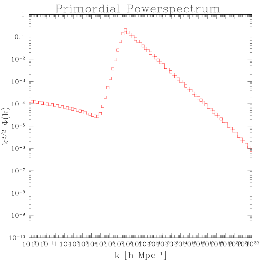
FIG. 1.: The spectrum of primordial fluctuations which produces the MACHO PBHs is depicted.

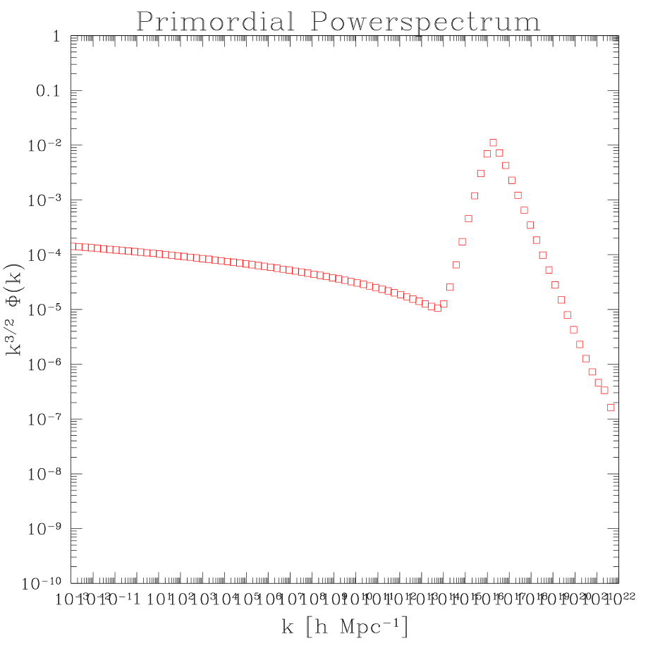
FIG. 2.: The spectrum of primordial fluctuations which produces the BESS (GRBs) PBHs is depicted.

REFERENCES

- [1]
- [2] See, for example, A. D. Linde, Particle Physics and Inflationary Cosmology (Harwood, Chur, Switzerland, 1990).
- [3] See, for a review, D. H. Lyth and A. Riotto, Phys. Rep. 314, 1 (1999).
- [4] See, for example, H. P. Nilles, Phys. Rep. 110, 1 (1984).
-
[5]
A. D. Linde,
Phys. Lett. 108B, 389 (1982);
A. Albrecht and P. J. Steinhardt, Phys. Rev. Lett. 48, 1220 (1982). - [6] T. Asaka, M. Kawasaki, and M. Yamaguchi, Phys. Rev. D 61, 027303 (2000).
- [7] K. I. Izawa, M. Kawasaki, and T. Yanagida, Phys. Lett. B 411, 249 (1997).
- [8] A. D. Linde, Phys. Lett. 129B, 177 (1983).
- [9] A. S. Goncharov and A. D. Linde, Phys. Lett. 139B, 27 (1984); Class. Quantum Grav. 1, L75 (1984).
- [10] H. Murayama, H, Suzuki, T. Yanagida, and J. Yokoyama, Phys. Rev. D 50, R2356 (1994).
- [11] M. Kawasaki, M. Yamaguchi, and T. Yanagida, Phys. Rev. Lett. 85, 3572 (2000); Phys. Rev. D 63, 103514 (2001).
- [12] M. Yamaguchi and J. Yokoyama, Phys. Rev. D 63, 043506 (2001).
- [13] G. Lazarides, C. Panagiotakopoulos, and N. D. Vlachos, Phys. Rev. D 54, 1369 (1996); G. Lazarides and N. D. Vlachos, ibid. 56, 4562 (1997); N. Tetradis, ibid. 57, 5997 (1998).
- [14] C. Panagiotakopoulos and N. Tetradis, Phys. Rev. D 59, 083502 (1999); G. Lazarides and N. Tetradis, ibid. 58, 123502 (1998).
-
[15]
L. A. Kofman, A. D. Linde, and A. A. Starobinsky,
Phys. Lett. 157B, 361 (1985);
J. Silk and M. S. Turner, Phys. Rev. D 35, 419 (1987);
D. Polarski and A. A. Starobinsky, Nucl. Phys. B385, 623 (1992);
P. Peter, D. Polarski, and A. A. Starobinsky, Phys. Rev. D 50, 4827 (1994);
S. Gottlöber, J. P. Mücket, and A. A. Starobinsky, Astrophys. J. 434, 417 (1994);
R. Kates, V. Müller, S. Gottlöber, J. P. Mücket, and J. Retzlaff, Mon. Not. R. Astron. Soc. 277, 1254 (1995);
D. Langlois, Phys. Rev. D 54, 2447 (1996); 59, 123512 (1999);
J. A. Adams, G. G. Ross, and S. Sarkar, Nucl. Phys. B503, 405 (1997);
J. Lesgourgues and D. Polarski, Phys. Rev. D 56, 6425 (1997);
J. Lesgourgues, D. Polarski, and A. A. Starobinsky, Mon. Not. R. Astron. Soc. 297, 769 (1998); M. Sakellariadou and N. Tetradis, hep-ph/9806461;
J. Lesgourgues, Phys. Lett. B 452, 15 (1999); Nucl. Phys. B582, 593 (2000);
T. Kanazawa, M. Kawasaki, N. Sugiyama, and T. Yanagida, Phys. Rev. D 61, 023517 (2000); astro-ph/0006445. -
[16]
P. de Bernardis et al.,
Nature (London) 404, 955 (2000);
A. E. Lange et al., Phys. Rev. D 63, 042001 (2001). -
[17]
S. Hanany et al.,
Astrophys. J. Lett. 545, L5 (2000);
A. Balbi et al., ibid. 545, 1 (2000). -
[18]
L. Randall, M. Soljacić, and A. H. Guth,
Nucl. Phys. B472, 377 (1996);
J. García-Bellido, A. D. Linde, and D. Wands, Phys. Rev. D 54, 6040 (1996). - [19] J. Yokoyama, Phys. Rev. D 58, 083510 (1998); 59, 107303 (1999).
-
[20]
M. Kawasaki, N. Sugiyama, and T. Yanagida,
Phys. Rev. D 57, 6050 (1998);
M. Kawasaki, and T. Yanagida, ibid. 59, 043512 (1999);
T. Kanazawa, M. Kawasaki, and T. Yanagida, Phys. Lett. B 482, 174 (2000). -
[21]
C. R. Alcock et al.,
Nature (London) 365, 621 (1993);
Phys. Rev. Lett. 74, 2867 (1995);
Astrophys. J. 486, 697 (1997);
E. Aubourg et al., Nature (London) 365, 623 (1993); Astron. Astrophys. 301, 1 (1995). - [22] K. Yoshimura et al., Phys. Rev. Lett. 75, 3792 (1995).
- [23] See, for example, D. B. Cline, C. Matthey, and S. Otwinowski, in Proceedings of the 14th IAP Colloquium (Frontieres, Paris, 1998), p. 374.
- [24] M. Yamaguchi, hep-ph/0103045.
- [25] G. ’t Hooft, in Recent Developments in Gauge Theories, edited by G. ’t Hooft et al. (Plenum, Cargèse, 1980).
- [26] A. D. Linde, Phys. Lett. B 175, 395 (1986); Mod. Phys. Lett. A 1, 81 (1986).
- [27] A. Vilenkin, Phys. Rev. D 27, 2848 (1983).
- [28] A. A. Starobinsky, in Current Topics in Field Theory, Quantum Gravity, and Strings, edited by H. J. de Vega and N. Sanchez, Lecture Notes in Physics Vol. 246 (Springer, Berlin, 1986), p. 107.
-
[29]
M. Yu. Khlopov and A. D. Linde,
Phys. Lett. 138B, 265 (1984);
J. Ellis, G. B. Gelmini, J. L. Lopez, D. V. Nanopoulos, and S. Sarker, Nucl. Phys. B373, 92 (1999);
M. Kawasaki and T. Moroi, Prog. Theor. Phys. 93, 879 (1995). - [30] D. Polarski and A. A. Starobinsky, Nucl. Phys. B385, 623 (1992); Phys. Rev. D 50, 6123 (1994); A. A. Starobinsky and J. Yokoyama, in Proceedings of the Fourth Workshop on General Relativity and Gravitation, edited by K. Nakao et al. (Kyoto University, Kyoto, 1994), p. 381.
- [31] C. L. Bennett et al., Astrophys. J. Lett. 464, L1 (1996).
- [32] B. J. Carr and S. W. Hawking, Mon. Not. R. Astron. Soc. 168, 399 (1974); B. J. Carr, Astrophys. J. 201, 1 (1975).
- [33] J. S. Bullock and J. R. Primack, Phys. Rev. D 55, 7423 (1997).
- [34] P. Ivanov, Phys. Rev. D 57, 7145 (1998).
- [35] D. S. Salopek, J. R. Bond, and J. M. Bardeen, Phys. Rev. D 40, 1753 (1989); J. Lesgourgues, Nucl. Phys. B582, 593 (2000); H. Suzuki, Master thesis, University of Tokyo, Japan, 1999.