Perfect Gauge Actions on
Anisotropic Lattices

Inauguraldissertation
der Philosophisch-naturwissenschaftlichen Fakultät
der Universität Bern

vorgelegt von

Philipp Rüfenacht

von Grosshöchstetten (BE)

Leiter der Arbeit: Prof. Dr. P. Hasenfratz Institut für theoretische Physik Universität Bern

Abstract and Summary

The theory of the strong interaction, Quantum Chromodynamics (QCD), may be studied using perturbation theory, the standard tool of quantum field theory, for high energies. Around 1 GeV, the scale of the hadronic world, however, the coupling constant is increased and perturbative methods fail. In this domain, Lattice QCD provides a systematic approach to the non-perturbative study of QCD. The theory is formulated on a discrete Euclidean space-time grid which non-perturbatively regularises QCD and allows for computer simulations of the theory using Monte Carlo methods.

The discretisation of the continuum action can be done in many different ways. Concerning the pure gauge sector of QCD, besides the standard discretisation, the Wilson action, there are several so-called improved actions which reduce artifacts coming from the discretisation. The most radical scheme of improving lattice actions, based on Wilson’s Renormalisation Group approach, has been suggested by Hasenfratz and Niedermayer, namely the creation of actions that are classically perfect, i.e. there are no lattice artifacts on the solutions of the lattice equations of motion.

In Lattice QCD, the energy of a physical state is measured studying the decay of correlators of creation and annihilation operators having an overlap with the state under consideration. If the state is heavy, these correlators decay very fast in time and one has to make sure that the temporal lattice spacing is small enough such that the signal of the correlator can be accurately traced over a few time slices before it disappears in the statistical noise. At the same time, one has to pay attention to choose the physical volume of the lattice large enough such that there are no significant finite-size effects. Both these requirements together lead to lattices with a large number of lattice sites, which means that it is computationally very expensive to perform the simulations. The obvious way out of this dilemma is to use a smaller lattice spacing in temporal direction compared to the spatial directions, i.e. using anisotropic lattices.

Anisotropic lattices have been widely used in the last few years. Studies comprising excited states of nucleons, heavy-quark bound states, heavy meson semi-leptonic decays, long range properties of the quark-antiquark potential as well as states composed purely of gluons (glueballs) or gluons and quarks (hybrids) have been performed, mainly using the standard Wilson discretisation of the anisotropic action or a mean-link and Symanzik improved anisotropic action. A classically perfect anisotropic action has still been absent.

It is thus the goal of this work to fill this gap, presenting a way of constructing classically perfect anisotropic gauge actions, building up on a recent parametrisation of the isotropic classically perfect action (FP action) that includes a rich structure of operators as it bases on plaquettes built from simple gauge links as well as from smeared links. The procedure leading to the anisotropic action is examined analytically on scalar fields as well as in the quadratic approximation for gauge fields. We then construct the $\xi=2$ action valid on coarse configurations occurring typically in Monte Carlo simulations. Its properties are studied performing measurements of the torelon dispersion relation (which serves as a means of determining the renormalisation of the bare (input) anisotropy), of the potential between a static quark and a static antiquark, of the deconfining phase transition and finally determining the spectrum of low-lying glueballs in pure gauge theory.

The feasibility of iterating the procedure, obtaining a classically perfect action with $\xi=4$, is briefly checked. Furthermore, we examine properties of the newly created anisotropic actions (as well as of the underlying isotropic action), such as autocorrelation times of different updates of the gauge configurations in the Monte Carlo simulation or the computational overhead of the classically perfect action compared to the widely-used mean-link and Symanzik improved action and to the standard Wilson gauge action.

It turns out that the construction of anisotropic classically perfect gauge actions is feasible. The iteration of the process yielding higher anisotropies seems to work as well. Measuring the renormalised anisotropy using the torelon dispersion relation turns out to be stable and unambiguous and shows that the renormalisation of the anisotropy is moderate and under good control. The measurements of the static quark-antiquark potential indicate that the violations of rotational symmetry are small if the (spatial) lattice is not exceptionally coarse. This shows that the parametrisation describes accurately the full action, which is known to have good properties concerning rotational symmetry. The study of the glueball spectrum is facilitated a lot due to the anisotropic nature of the action, even for (rather small) $\xi=2$. Reliable results, including continuum extrapolations, are obtained for glueball states having much larger mass than the highest-lying states that could have been resolved with the same amount of computational work using the isotropic action. However, the scaling properties of the glueball states, i.e. the behaviour of the measured energies as the lattice spacing is increased, seems to be rather unfavourable compared to the mean-link and Symanzik improved anisotropic action. Especially, this is the case for the lowest-lying scalar glueball which could be caused by the presence of a critical end point of a line of phase transitions in the fundamental-adjoint coupling plane assumed to define the continuum limit of a scalar field theory. Our action includes in its rich structure operators transforming according to the adjoint representation. If their coupling (which we do not control applying our method) lies in a certain region, the effect of the critical end-point on scalar quantities at certain lattice spacings (sometimes called the “scalar dip”) may even be enhanced compared to other (more standard) discretisations with purely fundamental operators. Concerning the cut-off effects observed in the glueball simulations, we have to add that other effects, such as effects due to the finite size of the lattices, may also be present and that this issue requires further study. Furthermore, the computational overhead of the classically perfect anisotropic action compared to the standard Wilson action and as well compared to the mean-link and Symanzik improved action is considerable and one has to weigh up the pros and cons carefully, if one is about to choose a gauge action for large-scale simulations.

Chapter 1 Introduction

This thesis covers work done in collaboration with Urs Wenger and Ferenc Niedermayer. Results already extensively discussed in Urs Wenger’s PhD thesis [1] that are necessary for the work presented here are briefly recapitulated. Parts of the results have already been published [2, 3, 4].

The aim of this Introduction is to motivate the work that has been done as well as to present the basic knowledge necessary for the subsequent Chapters.

1.1 Motivation

The most systematic approach to the non-perturbative study of QCD, the theory of strong interactions, is Lattice QCD (LQCD). The QCD action is discretised by putting the theory on a space-time lattice. As QCD, LQCD needs as input the quark masses and an overall scale. Then any Green’s function may be evaluated by taking averages of certain combinations of the lattice fields (measuring operators) on an ensemble of vacuum samples (lattice configurations). This allows the study of masses (spectroscopy) as well as the extraction of matrix elements. In contrast to the experiment, parameters such as quark masses, boundary conditions or sources may be arbitrarily varied in LQCD, which allows a wide range of studies to be contrasted with experimental results.

In order to measure the energies of states in LQCD, one studies the decay in time of correlators of respective operators. Thus the distance between lattice sites has to be small enough such that the signal of the correlators may be traced along several time-slices of the lattice before it disappears in the statistical noise. On the other hand, however, the physical size of the whole lattice has to be large enough such that there are no significant finite-size effects. Both these requirements together lead to lattices with a large number of lattice sites that are computationally expensive.

The obvious way out of this dilemma is the use of anisotropic lattices, whose spatial lattice spacing $a_{s}$, the distance between two neighbouring lattice sites in spatial direction, is larger than $a_{t}$, the one in temporal direction. The anisotropy or aspect ratio is conventionally denoted by $\xi=a_{s}/a_{t}$.

Anisotropic lattices have been widely used for studying heavy states in gauge theory for the last few years. For measurements in quenched QCD see e.g. [5] for $N^{*}$ masses, [6, 7, 8] for heavy quarkonia using relativistic heavy quarks, [9, 10, 11, 12, 13, 14] for heavy quarkonia including heavy hybrid states composed of quarks and glue or [15, 16] for heavy-light mesons employing NRQCD. Another work [17] has studied heavy meson semi-leptonic decays using NRQCD. Studies in pure $SU(3)$ gauge theory have mainly examined glueballs [18, 19, 20]. The study of string-breaking using static quarks in the adjoint representation [21] employed an anisotropic action to be able to have large spatial separations of the sources on a lattice with a moderate number of lattice sites. Other studies of static potentials including higher representations comprise works like [22, 23, 24, 25]. Anisotropic lattices have been also used to study (quenched) QCD at finite temperature [26, 27, 28, 29, 30] as the fine lattice in temporal direction allows for a fine variation of $T=1/(a_{t}N_{t})$ without the need of having to increase the number of spatial lattice sites. A study of the autocorrelation of spatial and temporal $SU(3)$ gauge operators on anisotropic lattices has been performed in [31]. Perturbative properties of improved anisotropic gauge and fermion actions, e.g. the dependence of the couplings $g_{s}$ and $g_{t}$ on $\xi$ as well as the ratio between the renormalised and the bare anisotropy $\eta=\xi_{\text{R}}/\xi_{0}$, have been studied in [32, 33, 34, 35]. Matching parameters for the study of matrix elements (mainly for heavy meson semi-leptonic decays) have been calculated in [36].

The discretisation of the continuum theory leads to cut-off effects (or lattice artifacts) in the results obtained on the lattice. These effects grow as the lattice spacing $a$ is increased (i.e. as the lattice gets more and more different from the continuum). As simulations using anisotropic actions are carried out on lattices where the spatial lattice is rather coarse — in order not to have too large cut-off effects it is advantageous to use improved discretisations of the continuum action suppressing such artifacts. Whereas it has been common to use improved anisotropic gauge actions for some years, above all in glueball simulations, the most radical concept of improving actions, the construction of classically perfect actions, has never been applied to this subject. It is thus the goal of this work to construct anisotropic classically perfect gauge actions and to examine their properties.

Different ways of constructing improved gauge actions are discussed in the remainder of this Chapter. On one hand, there are actions that are improved employing perturbation theory, on the other hand, the concept of renormalisation group provides means of improving actions non-perturbatively. One of the most radical ways of improving actions is the construction of the classically perfect Fixed Point action, which is described in detail in Sections 1.3.2 and 1.4.

In Chapter 2 we present some physical objects that may be studied in the context of pure lattice gauge theory and explain how we measure them in practice. The dispersion relation of the torelon is used to determine the renormalised anisotropy of the parametrised action as well as to provide an estimate for the scale at a given coupling $\beta$. The measurement of the critical temperature $T_{c}$ corresponding to the deconfining phase transition of pure gauge theory yields as well information about the (temporal) scale of a simulation. To determine the lattice spacing precisely as well as to obtain information about the rotational invariance of the parametrised FP action, we employ the static quark-antiquark potential. Finally, we describe bound states of pure glue, the glueballs, and discuss how they are measured on the lattice.

Chapter 3 contains a brief summary about the newly parametrised isotropic FP action [1, 2]. The action is presented as well as simulations studying the deconfining phase transition, the static quark-antiquark potential and glueballs. The scaling properties of the isotropic action are discussed as well.

In Chapter 4 we present the method used in this work to construct anisotropic classically perfect actions. Instead of repeating the whole construction programme as described at the end of this Chapter, we use the parametrised isotropic FP action and perform one single, purely spatial, blocking step to end up with a perfect anisotropic action with anisotropy $\xi=2$. Furthermore, we describe how the isotropic parametrisation using smeared links may be generalised such that it may as well account for the anisotropy between spatial and temporal directions.

This approach is then tested on free scalar fields that may be treated analytically as well as in the quadratic approximation of the FP action, as described in Chapter 5. It turns out that in both cases the ansatz works nicely.

The construction of the $\xi=2$ perfect action in full SU(3) gauge theory is presented in the next Chapter, including as well results of measurements of torelon energies , the static quark-antiquark potential, the critical temperature and the glueball spectrum.

Chapter 7 describes how the spatial blocking step may be repeated to obtain actions with larger anisotropies and presents first results about the renormalised anisotropy of the $\xi=4$ perfect action. It turns out that the iteration of the spatial blocking step seems to be feasible and poses no additional difficulties.

In Chapter 8 we present results of measurements of autocorrelation times as well as information about the overhead to be expected in simulations using the perfect anisotropic actions compared to the standard Wilson action.

Conclusions and prospects are given in Chapter 9.

1.2 Perturbatively Improved Gauge Actions

On very smooth lattice configurations, i.e. configurations with a very small lattice spacing $a$ close to the continuum, any discretisation of the continuum gauge action yields basically the same results, the leading lattice artifacts of $O(a^{2})$ are very small. Increasing the lattice spacing $a$, the form of the discretisation gets more and more important and simple discretisations of the continuum action (e.g. the Wilson action) may lead to large cut-off effects. It is thus favourable to use more sophisticated — improved — actions that suppress the lattice artifacts. There exist several ways of constructing improved actions, in the next few sections we present the most important ones that are used for lattice gauge theories.

One method to construct improved actions is following Symanzik’s proposal [37, 38], killing the lattice artifacts order by order in $a^{2}$, adding operators of corresponding dimensions that cancel the artifacts. This yields e.g. the well known Lüscher-Weisz action [39] which has leading corrections at $O(g^{4}a^{4})$.

A technique very important in the context of this work is mean-field (or tadpole) improvement which helps to calculate perturbative coefficients, as those appearing in Symanzik improved actions, more reliably. This is achieved by changing the set up for lattice perturbation theory. On the lattice, gauge fields are represented in the following way:

$$U_{\mu}(x)=e^{iagA_{\mu}(x)}=1+iagA_{\mu}(x)-\frac{a^{2}g^{2}}{2}A_{\mu}^{2}(x)+\cdots,$$ (1.1)

where $U_{\mu}(x)$ is the gauge link at lattice site $x$. This form obviously gives rise to local quark-gluon vertices with 1, 2, $\ldots$ gluons. All these vertices except the lowest one are lattice artifacts. Contracting the two gluons in the term $a^{2}g^{2}A_{\mu}^{2}(x)/2$ one obtains so-called tadpole diagrams. As it was recognised by Parisi [40] and later by Lepage and Mackenzie [41] these artifacts are in fact only suppressed by powers of $g^{2}$ as the ultraviolet divergences generated by the tadpole loops kill the $a^{2}$ suppressions. These contributions are made responsible for the poor match between short distance quantities and their perturbative estimates as well as for large coefficients occurring in perturbative lattice expansions.

Mean-field (or tadpole) improvement has been proposed to get rid of this kind of artifacts. It assumes that the lattice fields can be split into an ultraviolet (UV) and an infrared (IR) part and that the UV part should be integrated out [40, 41]:

$$e^{iagA_{\mu}(x)}=e^{iag(A_{\mu}^{\text{IR}}(x)+A_{\mu}^{\text{UV}}(x))}=u_{0}e^{iagA_{\mu}^{\text{IR}}(x)}\equiv u_{0}\tilde{U}_{\mu}(x).$$ (1.2)

It just amounts to a simple rescaling of the link variables $U_{\mu}(x)$ by an overall constant factor $u_{0}<1$. Instead of the common expansion parameters, the coupling $g^{2}$, the hopping parameter $\kappa$ in the fermion action and the links $U$ one uses their improved counterparts $\tilde{g}^{2}=g^{2}/u_{0}^{4}$, $\tilde{\kappa}=\kappa u_{0}$ and $\tilde{U}=U/u_{0}$. There are two common choices for the tadpole factor $u_{0}$, either the fourth root of the plaquette expectation value or the expectation value of the link in Landau gauge. Tadpole improvement may be especially useful for the construction of anisotropic actions because it leads to a small renormalisation of the anisotropy $\xi$, if this quantity is introduced perturbatively, as e.g. in Symanzik improved anisotropic actions. Indeed, the anisotropic action most widely used [5, 9, 10, 11, 12, 13, 14, 15, 16, 17, 18, 19, 20, 21, 24, 25, 31, 36] in the last few years, initially presented in [42], combines mean-link and Symanzik improvement (at tree-level).

Other, non-perturbative methods of improving actions base on the renormalisation group. This concept, as well as resulting actions are briefly introduced in the next section.

1.3 The Renormalisation Group

A Field Theory is defined over a large range of scales from small, physical energies up to the cut-off that is sent to infinity to reach the continuum limit. The fields associated with very high (unphysical) scales do influence the physical predictions indirectly through a complex cascade process; however no physical question involves them directly. This makes the connection between the local form of the interaction and the final predictions obscure. Additionally, the large number of degrees of freedom present makes the problem technically difficult. That is why one attempts to integrate out these non-physical high momentum scales in the path integral. The method accomplishing this, taking into account the effect on the remaining variables exactly, is called the Renormalisation Group transformation (RGT) [43, 44, 45, 46, 47, 48, 49, 50].

Figure 1.1: Schematic flow diagram for asymptotically free theories.

The sequence of theories defined by the repeated use of the RGT on an initial theory defines a flow trajectory in the space of couplings. Fixed points (FPs) of this transformation are theories that reproduce itself under the RGT. Since the correlation length of the theory scales by the scaling factor of the RGT, its value has to be 0 or $\infty$ at the fixed point. In Yang-Mills theory there is a non-trivial fixed point (the Gaussian FP) with correlation length $\xi=\infty$ whose exact location in coupling space $c_{1}$, $c_{2},\ldots$ depends on the RGT used. There is one so-called “relevant” coupling whose strength increases as one is starting at this FP and performing RGTs. The flow along this relevant scaling field whose end-point is the FP is called the renormalised trajectory (RT). This situation is sketched in Figure 1.1 Simulations performed using an action which is on the exact RT reproduce continuum physics without any discretisation errors.

There are different approaches to take advantage of this knowledge about field theories in the vicinity of a fixed point, presented in the next two sections.

1.3.1 Renormalisation Group Improved Actions

Iwasaki [51] has studied RGTs in perturbation theory and has obtained a gauge action using two loop-shapes that after a few blockings comes close to the RT. It shows better rotational invariance and better scaling of $T_{c}/\sqrt{\sigma}$ than the standard action. Today, this action is used e.g. by the CP-PACS collaboration for MC simulations including domain-wall fermions [52] as it turned out that the Iwasaki action shows better behaviour concerning chiral symmetry.

Gupta and Patel [53] have studied the flow of a scale $\sqrt{3}$ RGT and approximate the action using four parameters and two loop shapes in different representations. Studies of lattice topology have shown that short distance artifacts are suppressed [54, 55].

The QCD-TARO collaboration [56, 57] has examined the flow of a scale 2 RGT and evaluated the couplings on blocked lattices using Schwinger-Dyson equations. The blocked action is reproduced by two couplings corresponding to the simplest Wilson plaquettes $1\times 1$ and $1\times 2$.

1.3.2 The Classically Perfect FP Action

Another, more radical, method has been suggested by Hasenfratz and Niedermayer [58]: For asymptotically free theories like SU($N$) Yang-Mills theory, the action at the FP where the (only) relevant coupling $g=0$ (corresponding to $\beta=\infty$) may be determined using a saddle-point equation. The FP action is classically perfect, i.e. there are no lattice artifacts on the solutions of the lattice equations of motion. This is equivalent to an on-shell Symanzik improvement at tree-level to all orders in $a$.

Let us consider SU($N$) pure gauge theory in $d=4$ Euclidean space-time on a periodic lattice. The partition function reads

$$Z(\beta)=\int dUe^{-\beta{\cal A}(U)},$$ (1.3)

where $dU$ is the invariant group measure and ${\cal A}(U)$ a discretisation of the continuum action. We perform a real space RGT:

$$e^{-\beta^{\prime}{\cal A}^{\prime}(V)}=\int dU\exp\left\{-\beta({\cal A}(U)+T(U,V))\right\},$$ (1.4)

where $V$ is the blocked link variable and $T(U,V)$ is the blocking kernel defining the explicit form of the transformation. As for asymptotically free theories the FP lies at $\beta=\infty$, in this limit the path integral can be calculated in the saddle-point approximation. This leads to an equation in classical field theory defining the FP action which is mapped onto itself by the RGT:

$${\cal A}^{\text{FP}}(V)=\min_{\{U\}}\left\{{\cal A}^{\text{FP}}(U)+T(U,V)\right\}.$$ (1.5)

1.4 The Construction of a FP Action for Coarse Configurations

The FP saddle point equation 1.5 derived in the last section may be studied analytically up to quadratic order in the vector potentials [59, 60] (see Section 5.2). However for solving the FP equation on coarse configurations one has to resort to numerical methods. Additionally, although the full FP action is local, it is described in principle by infinitely many couplings that decrease exponentially with the space-time separation of the two coupled variables in the action. In order to use a FP action in a numerical simulation it thus has to be approximated by some parametrisation with a finite number of couplings.

1.4.1 The Method Used

The construction of the FP action on rough configuration relies on the observation that the fluctuations of the minimising configurations $U$ in eq. 1.5 are reduced by a factor of 30 to 40 compared to the initial coarse fields $V$. That is why after a small number of inverse RGTs (calculating the minimising configurations $U$ corresponding to coarser configurations $V$, i.e. using eq. 1.5 as a recursion relation linking two actions $\mathcal{A}$, $\mathcal{A}^{\prime}$) the configurations are so smooth that they can be described accurately by a simple discretisation of the gauge action, e.g. the Wilson action. In practise it is not feasible to perform the necessary number of RG steps at once due to memory and computer time limitations, we therefore resort to a cascade process involving several single RG steps of first inverse blocking coarse configurations and then parametrising the action on these configurations using eq. 1.5. This idea is displayed in Figure 1.2. In the following sections we describe the starting point of the procedure, i.e. a simple discretisation of the action for smooth fields, as well as the proceeding to parametrise actions $\mathcal{A}(V)$ at intermediate and final levels, using eq. 1.5.

Figure 1.2: The cascade procedure used to obtain perfect actions for strongly fluctuating fields $V_{2}$ starting with a simple action $\mathcal{A}_{0}$ suitable for very smooth configurations $U_{0}$. Coarse configurations $V_{2}$ (on the level of MC simulations), $V_{1}$, $V_{0}$; fine configurations $U_{2}$, $U_{1}$, $U_{0}$ (of which the latter may be described with the staring action $\mathcal{A}_{0}$). The boxes contain configurations on the same level of fluctuations. The actions $\mathcal{A}$ describing the respective configurations are also indicated. Note, that the number of steps actually used may differ from the number displayed in this Figure.

1.4.2 The Starting Point

As a starting point, we use very fine configurations (corresponding to “$U_{0}$” in Figure 1.2) that are described well by a simple action. As an example, for the parametrisation of the isotropic action we generate coarse configurations (“$V_{0}$”) where the plaquette variable $u(V_{0}(n_{B}))\leq 0.25$ for all $n_{B}$ and thus for the corresponding minimised configurations $u(U_{0}(n))\leq 0.009$ for all $n$. These fine configurations can be accurately described by the quadratic approximation of the FP action fulfilling the $O(a^{2})$ Symanzik condition, denoted by $\mathcal{A}_{0}$ [1, 2].

To check how well this action $\mathcal{A}_{0}$ is working on the minimised configurations, we generate a set of configurations showing fluctuations of the same magnitude and corresponding configurations which are identical up to one link which is changed. The change of the action due to this changed link may then be calculated on one hand using the parametrisation $\mathcal{A}_{0}$, on the other hand we minimise all the configurations and use the r.h.s. of eq. 1.5 which rests upon the action on the minimised configurations whose fluctuations are again smaller by a factor of 30–40, i.e. this result is expected to be very close to the exact one. The difference of these two action values is thus a good estimate of the error of the parametrisation. It turns out that the typical error is about 1–2% only.

We may now use eq. 1.5 to fix the parameters of an appropriate parametrisation of the action $\mathcal{A}_{1}$ valid on configurations with $u(V_{0})\leq 0.25$.

This process is now repeated with coarser configurations ($V_{1}$) whose minimised counterparts ($U_{1}$) show fluctuations $u(U_{1})\leq 0.25$, describing these minimised configurations on the r.h.s. of eq. 1.5 by the action $\mathcal{A}_{1}$. It turns out that step by step the complexity of the parametrisation (i.e. the number of free parameters) has to be increased in order to be able to describe the action well on the coarser and coarser fields.

1.4.3 Quantities to be Fitted

Performing the numerical minimisation of the configurations $V$ is an expensive task, even for small configurations. It is thus very useful to be able to fit not only one quantity per configuration (the total action $\mathcal{A}(V)$) but to include as well the derivatives of the gauge action with respect to the gauge links in a given colour direction $a$:

$$\frac{\delta\mathcal{A}(V)}{\delta V_{\mu}^{a}(n)},\quad\mu=1,\ldots,4,\quad a=1,\ldots,N_{c}^{2}-1,$$ (1.6)

where $N_{c}$ denotes the number of colours. These quantities are easily accessible and deliver $V\cdot(N_{c}^{2}-1)\cdot 4$ additional residues for the fit per configuration. It is understood that these quantities are not completely independent, but still the increase of useful data per configuration is dramatic.

The intermediate actions $\mathcal{A}_{1}$, $\mathcal{A}_{2}$ etc. still fulfill the $O(a^{2})$ Symanzik conditions in order to be valid as well for configurations with smaller fluctuations — however, in the last step yielding the final parametrisation of the FP action for coarse fields, this requirement is dropped to get an effective FP action describing well the typical MC configurations using a compact set of parameters. Additionally, we include scale-invariant instanton solutions [61, 62, 63, 64] to make the action performing well concerning topology.

Adjusting the weights of the different quantities entering into the fit, we may tune the importance of the respective quantity in the determination of the action, see also Section 1.4.5

In the last step we include into the fit several sets of 10–40 configurations each at different values of the coupling $\beta$ to obtain a parametrisation which is valid on a certain range of couplings suitable for MC simulations.

In the following Sections we describe the steps performed to parametrise a perfect action at a certain level of the cascade procedure.

1.4.4 The Non-Linear Fit

Before we may describe the actual fitting procedure used for the parametrisation of the isotropic FP action as well as for the perfect anisotropic actions, let us briefly explain some of the main features of our parametrisation for perfect actions. For a more detailed account on this issue, see Section 4.3.

The action is a mixed polynomial of traces of simple loops (plaquettes) built from simple gauge links as well as from (APE-like) smeared links. The parameters in the smearing enter the fitting procedure non-linearly, the parameters in the polynomial enter the fit linearly. This distinction is crucial for the following description of the actual fitting process. The main advantage of this parametrisation ansatz is the rich structure including a large number of different loops at moderate computational cost; however, the couplings of the loops in the action are not independent from each other but complicated combinations of the non-linear and linear parameters appearing in our parametrisation.

First we perform a full non-linear $\chi^{2}$ fit varying the non-linear parameters describing the smearing as well as the linear parameters accounting for the composition of the action in terms of simple and smeared plaquettes. The linear part of the fit is performed exactly, its computational cost is negligible. The non-linear part is done using a Simplex algorithm which is rather slow, however the danger of missing the true minimum is small. A rough estimate of the number $N$ of non-linear fitting steps (where every step includes the recalculation of all the residues) as a function of the number $n_{\text{nl}}$ of non-linear parameters is

$$N=50(20)e^{0.23(4)n_{\text{nl}}}.$$ (1.7)

Due to this behaviour ($N$ increases roughly by a factor of 10 for 10 additional non-linear parameters), it is not easily possible to increase the number of free non-linear parameters above $15\sim 20$ in the full non-linear fit.

The non-linear fit is performed for different sized sets of non-zero non-linear parameters with a (fixed) large number of free linear parameters. The only quantities fitted at this stage are the derivatives of the action with respect to the coarse couplings to obtain a “basic” value of $\chi^{2}$ which may be used to estimate the quality of the fits in the next step where additional quantities are taken into account or the number of linear parameters is decreased. Restrictions such as the norm of the action or Symanzik conditions are applied already to the non-linear fit, however.

The number and the values of non-linear parameters of the parametrised action are fixed looking at the $\chi^{2}$ of the fit — which in principle is rather delicate, as it is unknown whether e.g. a 10 % decrease of $\chi^{2}$ when introducing an additional free parameter is a sign of importance of this extension or whether this set is already large enough to account for the FP nature of the action. These questions can be answered only at the end of the whole procedure when the final parametrisation is checked on physical quantities. However, whether the parametrisation is stable, i.e. whether the number of data points is already large enough to account for a parametrisation that does not depend on the actual configurations in the fit, may be — and has to be — checked after the non-linear fit, measuring $\chi^{2}$ on independent sets of configurations.

# $\eta$	# $c_{i}$	$i$	$\max(k+l)_{\text{sp}}$	$\max(k+l)_{\text{tm}}$	$\chi_{\text{d}}^{2}$	$\xi_{\text{R}}$
4	1	4	4	4	0.0250	1.63(2)
2	3	3	4	4	0.0238
4	3	3	4	4	0.0144	1.912(9)

Table 1.1: Example for the behaviour of $\chi^{2}$ in the full non-linear fit (for the $\xi=2$ perfect action), depending on the number (and kind) of non-linear parameters. Values of the (physical) renormalised anisotropy $\xi_{\text{R}}$ measured later are also given.

To give an example, we copy Table 1.1 from Section 4.3.4. In this case, the 40% decrease of $\chi^{2}$ between the # $c_{i}$ = 1 and the # $c_{i}$ = 3 non-linear parameter set (see Section 4.3 for an explanation) seems to be vital for an appropriate parametrisation of the perfect action as the renormalised anisotropy $\xi_{\text{R}}$ of the first parametrisation deviates considerably from the input value $\xi=2$ whereas the renormalisation is small for the second, more sophisticated, parametrisation.

1.4.5 The Linear Fit

Having at hand the set of non-linear parameters we may proceed performing fast linear fitting steps. The action values of the configurations as well as additional data such as the action of scale-invariant instanton solutions are included at this stage. The stability of $\chi^{2}$ is an indication of the ability of the chosen parameter set to incorporate additional information. At the same time the number of linear parameters may be decreased until $\chi^{2}$ starts to rise considerably. Figure 1.3 displays the change of $\chi^{2}$ (for the derivatives and the action values of 20 configurations at $\beta=3.5$ and $\beta=4.0$, respectively) if one changes the weight of the action value residues compared to the (fixed) weight of the derivatives. The value of $w_{\text{act}}$ finally used is marked by the dotted line. This choice preserves the good value of $\chi^{2}$ for the derivatives up to a few per cent while $\chi^{2}$ of the action values is about twice the minimum value reachable with a very large weight. Without inclusion of the action values into the fit, the average relative error of the parametrised action compared to the true one amounts to about 10%, with the weight chosen to about 0.5% and with infinite weight it might be decreased to about 0.2% (destroying the good parametrisation of the derivatives completely).

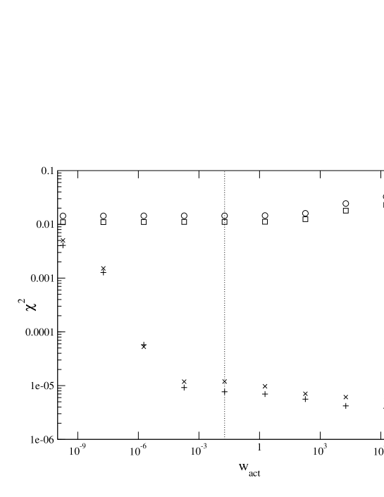
Figure 1.3: The effect of changing $w_{\text{act}}$, the weight of the action compared to the weight of the derivatives, in the linear fit for the $\xi=2$ perfect action. The values of $\chi^{2}$ for the derivatives of $\beta=3.5$ (circles) and $\beta=4.0$ (boxes) configurations as well as for the action values of $\beta=3.5$ (pluses) and $\beta=4.0$ (crosses) configurations are given. The dotted line marks the final choice of the relative weight $w_{\text{act}}$. The number of parameters remains fixed.

However, in the last step of the cascade process, when one aims at parametrising the final action to be used in MC simulations, the main difficulty of the choice of the linear set to be used is the behaviour of the parametrised action in terms of the simple and smeared plaquettes of the configurations, determined by the linear parameters. It happens that all the data in the fit is properly described by the parameters, but that varying the simple or smeared plaquette value slightly above or below the values occurring in the fit results in fake negative contributions to the action. In a MC simulation, this is a very dangerous behaviour as this might result in configurations with an artificial structure, i.e. the algorithm could try to maximise the number of plaquettes having a negative contribution to the action etc. One thus has to study the linear behaviour of the action, e.g. looking at plots of the action contribution vs. the values of the simple plaquette $u$ (which is bounded, $0\leq u\leq 4.5$) and the smeared plaquette $w$ (which in principle is unbounded as $w$ is not projected to SU(3)). It may be that accidentally none of the parametrisations behaves well enough for MC simulations. This is especially the case if conditions on the linear parameters, such as the norm of the action, that are determined by the values of the non-linear parameters lead to the bad behaviour of the linear part of the action. In this case we include a number of constraints $\mathcal{A}(u,w)>0$ (for different pairs of $(u,w)$ at the edge of the $(u,w)$-region expected to occur in MC simulations) into the non-linear fit in order to get a different set of non-linear parameters allowing for linear parameters with a good behaviour. (Generally in the space of non-linear parameters several almost degenerate minima in $\chi^{2}$ exist for very different sets of parameters, so this does not result in a significant rise of $\chi^{2}$ (of course, this has to be checked). It turns out that the best way of introducing these constraints into the non–linear Simplex minimisation is adding the absolute value of negative contributions to the action at the $(u,w)$ pairs multiplied with a large factor (we use $10^{6}$). “Hard” constraints with a step function at $\mathcal{A}(u,w)<0$ may lead to failure of the simplex algorithm as in this case it is not directed towards the region of the parameter space, where the action is behaving as desired.

Figures 1.4 and 1.5 show linear sets behaving badly and well. These examples are taken from the fit of the $\xi=4$ perfect action (see Chapter 7) where it is necessary to force several points $(u,w)$ in the non-linear fit to result in a positive contribution to the action. The first figure (standard non-linear fit) shows that in this case the spatial linear parameters lead to negative contributions of spatial plaquettes in a large region of $(u,w)$ values whereas the temporal part of the action is o.k. The second figure shows the behaviour of the parameters finally chosen, where conditions on the action contributions are included into the non-linear fit. There are no dangerous regions with negative contributions to the action. Pilot MC runs prove that indeed no abnormal behaviour of the action is observed.

\psfrag{action}{$\mathcal{A}(u,w)$}\psfrag{u}{$u$}\psfrag{w}{$w$}\includegraphics[width=227.62204pt]{sp_bad.eps}

\psfrag{action}{$\mathcal{A}(u,w)$}\psfrag{u}{$u$}\psfrag{w}{$w$}\includegraphics[width=227.62204pt]{tm_bad.eps}

Figure 1.4: A linear set of parameters with bad behaviour (danger of generating artificial configurations with a lot of negatively contributing plaquettes in a MC run). Upper plot: Spatial parameters, lower plot: temporal parameters.

\psfrag{action}{$\mathcal{A}(u,w)$}\psfrag{u}{$u$}\psfrag{w}{$w$}\includegraphics[width=227.62204pt]{sp_good.eps}

\psfrag{action}{$\mathcal{A}(u,w)$}\psfrag{u}{$u$}\psfrag{w}{$w$}\includegraphics[width=227.62204pt]{tm_good.eps}

Figure 1.5: A linear set of parameters with good behaviour. Upper plot: Spatial parameters, lower plot: temporal parameters.

Chapter 2 Physical Objects in Pure Lattice Gauge Theory

There are several interesting objects existing in pure gauge theory that can be studied non-perturbatively on the lattice. Some of them, the ones we study by Monte Carlo simulation, are presented in this chapter, together with experimental results (if present). They comprise the torelon (including non-zero momenta), the deconfining phase transition, the static quark-antiquark potential and glueballs. Furthermore, we explain how these states are measured on the lattice and what techniques we use to determine the energies of the states or the critical temperature of the phase transition respectively. For the results of the simulations we refer to Chapter 3 for a recapitulation of results obtained using the isotropic FP action, to Chapter 6 for $\xi=a_{s}/a_{t}=2$ perfect action results and to Chapter 7 for first results obtained with the $\xi=4$ perfect action.

2.1 The Torelon

2.1.1 Torelons in the Continuum

The torelon is a closed gluon flux tube encircling the periodic spatial boundary of size $L$ of a torus. It is created and annihilated by closed gauge operators winding around this boundary, see Figure 2.1.

Figure 2.1: A creation operator for torelons.

String models which are a good approximation for long flux tubes predict its energy to behave as

$$E(L)=\sigma L+\frac{\pi}{3L},$$ (2.1)

where $\sigma$ is the string tension and the second term describes the string fluctuation for a bosonic string [65, 66, 67, 68]. In contrast to the static quark-antiquark potential (see Section 2.3) where the string models the gluon flux between static colour sources, there is no Coulomb part corresponding to gluon exchange. The string models assume no restriction on the transverse modes of the string, the transverse extension $S$ of the volume thus has to be large enough in order to be able to apply their predictions.

To learn more about QCD in a finite volume, see [69].

2.1.2 Torelons on the Lattice

On the periodic lattice, a torelon associated to a point in the $(x,y)$-plane is created by a Polyakov loop winding around the lattice in $z$ direction starting at that point. Because of the relatively small lattice sizes necessary and the rather simple operators that can be used, torelon measurements on the lattice have quite a long history [70, 71, 72, 73, 74, 75, 76, 77, 78, 79]. In order to be able to compare the results to string models as well as not to have too large transverse momenta we choose to work on an $S^{2}\times L\times T$ lattice where $S$ and $T$ are large, whereas the length of the $z$-direction $L$ is chosen to be rather short, because long torelons are more difficult to measure due to their higher energies (see eq. 2.1).

As the colour flux is wandering as it loops around the lattice, it is useful to employ (iteratively) APE smeared links [80] to model this, which improves the overlap of the operators with the ground state. One step of APE smearing acts on a gauge link $U_{j}(x)$ as

$${\cal S}_{1}U_{j}(x) \equiv {\cal P}_{\text{SU(3)}}\Big{\{}U_{j}(x)+\lambda_{s}\sum_{k\neq j}(U_{k}(x)U_{j}(x+\hat{k})U_{k}^{\dagger}(x+\hat{j})$$

$$\hskip 56.9055pt+U_{k}^{\dagger}(x-\hat{k})U_{j}(x-\hat{k})U_{k}(x-\hat{k}+\hat{j}))\Big{\}},$$

the original link variable is replaced by itself plus a sum of the four neighbouring spatial staples and then projected back to SU(3). The smeared and projected links $S_{1}U_{j}(x)$ have the same symmetry properties under gauge transformations, charge conjugations or reflections and permutations of the coordinate axes. The smearing is used iteratively allowing to measure operators on configurations of different smearing levels, ${\cal S}_{n}U$.

We thus measure the operators

$$T_{n}(x,y,t)=\text{Tr}\prod_{z=0}^{L-1}{\cal S}_{n}U_{z}(x,y,z,t),$$ (2.3)

for all $x$, $y$, $t$, where ${\cal S}_{n}U_{z}$ is the $n$ times iteratively smeared link in the longitudinal $z$ direction. By discrete Fourier transform, we project out the state with momentum $\mathbf{p}=(p_{x},p_{y})=(n_{x},n_{y})(2\pi/Sa_{s})$:

$$T_{n}(\mathbf{p},t)=\sum_{x,y}T_{n}(x,y,t)e^{i(p_{x}x+p_{y}y)}$$ (2.4)

and build the correlators

$$C_{nn^{\prime}}(\mathbf{p},t)=\frac{1}{N_{t}}\sum_{\tau}\langle T_{n}(\mathbf{p},\tau)T_{n^{\prime}}(\mathbf{p},\tau+t)\rangle.$$ (2.5)

Using these correlators of operators measured on the different smearing levels we obtain the energy values $a_{t}E(\mathbf{p})$ employing variational methods (see Appendix E). The continuum dispersion relation

$$E^{2}=\mathbf{p}^{2}+m^{2}$$ (2.6)

on the lattice becomes (in temporal units)

$$(a_{t}E)^{2}=a_{t}^{2}(\mathbf{p}^{2}+m^{2})=\frac{(a_{s}\mathbf{p})^{2}}{\xi_{\text{R}}^{2}}+(ma_{t})^{2}=\frac{1}{\xi_{\text{R}}^{2}}(n_{x}^{2}+n_{y}^{2})\left(\frac{2\pi}{S}\right)^{2}+(ma_{t})^{2},$$ (2.7)

where $n_{x}$, $n_{y}$ are the components of the (transversal) lattice momentum. On an anisotropic lattice, this equation allows for the extraction of the renormalised anisotropy $\xi_{\text{R}}=a_{s}/a_{t}$ (measuring the “renormalisation of the speed of light”) as well as the torelon mass $ma_{t}$, which in turn may be used to get an estimate of the scale using eq. 2.1 and known values of the string tension $\sigma$.

2.2 The Deconfining Phase Transition

Pure lattice gauge theory is invariant under a global unitary transformation which transforms all temporal links $U_{4}(\vec{x},t)$ of a given timeslice (fixed $t$) as

$$U_{4}(\vec{x},t)\longrightarrow zU_{4}(\vec{x},t),$$ (2.8)

where $z$ is an element of the center $\mathcal{Z}(N_{c})$ of the gauge group SU($N_{c}$). For SU(3), $z=\exp(2\pi il/3)$, $l=$0, 1, 2.

To study this symmetry, we look at the Polyakov loop (or Wilson line)

$$P(\vec{x})\equiv\text{Tr}\prod_{t=0}^{N_{t}-1}U_{4}(\vec{x},t),$$ (2.9)

which is a loop wrapping around the lattice in temporal direction, representing a single static quark at finite temperature, as the temperature $T$ is proportional to the inverse of the temporal extension $N_{t}$, $T\propto 1/N_{t}$.

The correlation of the Polyakov loop $P(\vec{x})$ and its adjoint $P^{\dagger}(0)$ is related to the free energy $F_{q\bar{q}}$ of a static quark separated from a static antiquark by the distance $\vec{x}$ according to

$$\langle P(\vec{x})P^{\dagger}(0)\rangle\mbox{ }\propto\mbox{ }\exp(-F_{q\bar{q}}/T),$$ (2.10)

where $T$ denotes the temperature. For large separation, cluster decomposition requires

$$\langle P(\vec{x})P^{\dagger}(0)\rangle\longrightarrow|\langle P(0)\rangle|^{2}.$$ (2.11)

For low temperatures below the critical temperature, $T<T_{c}$, center symmetry holds and thus $\langle P(0)\rangle=0$ which allows for increasing $F_{q\bar{q}}(\vec{x})$ with growing distance $|\vec{x}|$, the static quarks are confined. For temperatures above $T_{c}$, center symmetry is broken, $\langle P(0)\rangle\neq 0$ and thus the free energy of the static quarks has to vanish, $F_{q\bar{q}}(\vec{x})\equiv 0$, the quarks are free and form, together with the gauge degrees of freedom, the quark-gluon plasma.

Figure 2.2 displays the distribution of the Polyakov loop for different couplings $\beta$ (for the $\xi=2$ perfect action, see Chapter 6). The critical coupling on the lattice used has been determined to $\beta_{c}=3.118(1)$. It is clearly visible that below the critical coupling the Polyakov loop values are close to zero whereas above $\beta_{c}$ they choose one of the three degenerate vacua. The coexistence of the two phases may be observed in the plot for $\beta=3.12$ which is very close to $\beta_{c}$.

The critical temperature $T_{c}$ may be determined by the location of the peak in the susceptibility

$$\chi\equiv N_{s}^{3}(\langle|P|^{2}\rangle-\langle|P|\rangle^{2}).$$ (2.12)

There is strong evidence for this transition to be first order for SU(3) [81, 82, 83, 84, 85], however in finite volume (on lattices used in MC calculations) the $\delta$-peak of the susceptibility $\chi$ is washed out and limits the precision with which one may determine the critical temperature $T_{c}$ or, equivalently, the critical coupling $\beta_{c}$ corresponding to a fixed temporal extension $L_{t}=aN_{t}$ of the lattice.

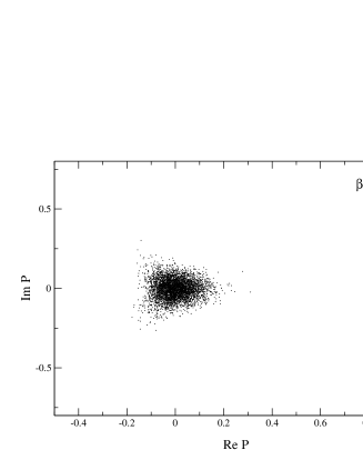
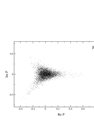
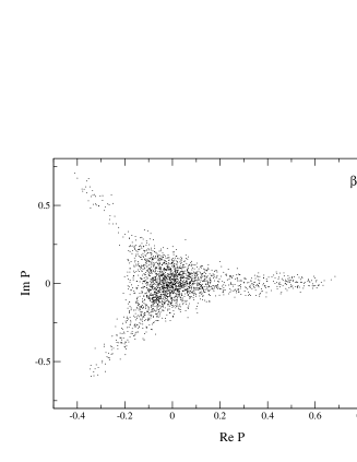
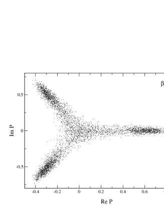
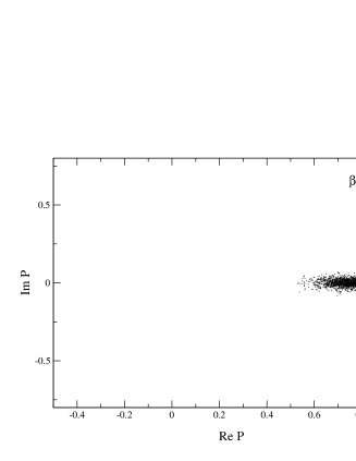
Figure 2.2: The distribution of the Polyakov loop at different couplings $\beta$ for the $\xi=2$ perfect action, $N_{t}=5$, $N_{s}=9$. The critical value of the coupling has been determined to $\beta_{c}=3.118(1)$. The system is heated up such that the center symmetry is broken as $\beta>\beta_{c}$. For clearness, only (randomly chosen) 10% of the data are displayed.

2.2.1 Determining the Peak of the Susceptibility

As mentioned in the last section, the critical coupling $\beta_{c}$ is determined by locating the peak of the susceptibility $\chi$ (eq. 2.12). To accomplish this, simulations at different values of $\beta$ near the estimated critical coupling $\beta_{c}$ have to be performed. For all these simulations a certain statistics has to be reached and it may thus be very time consuming to approach $\beta_{c}$ closer and closer performing simulations at more and more values of $\beta$. As the Monte Carlo simulation may exhibit critical slowing down, i.e. a dramatic rise of the autocorrelation times (see Section 8.1) near the phase transition, the procedure gets even more expensive. A nice solution to this problem is the use of reweighting techniques that allow extrapolating or interpolating results obtained at a given coupling or temperature to other (rather close) values of these parameters. To determine the peak of the Polyakov loop susceptibility we employ Ferrenberg-Swendsen reweighting [86, 87] and thus present the main idea of this procedure very briefly (for a more extensive presentation, see Appendix C of [1]).

All the information about a statistical system at temperature $T$ is contained in the partition function

$$Z(\beta)=\sum_{\{\sigma\}}e^{-\beta S(\sigma)},$$ (2.13)

where $\{\sigma\}$ denotes the set of all possible configurations of the system, $S(\sigma)$ is the energy for a given configuration $\sigma$. The same partition function may be written as

$$Z(\beta)=\sum_{S}W(S)e^{-\beta S},$$ (2.14)

where $W(S)$ is the density of states at the energy $S$, also called spectral density function. This function is universal, it is the same function for every temperature and thus contains in principle all the information about the system at any temperature $T$. In practice, our numerical results at a given value of $\beta$ will allow us to estimate $W(S)$ only for a finite range of energies $S$ occurring often enough in simulations at the given coupling. However, if we are studying a phase transition, due to the broad probability distribution of the examined states in simulations near criticality, $\beta$ being close enough to $\beta_{c}$, it is possible to estimate the spectral density function in a large range of energies.

Let us now consider $n$ measurements of an observable obtained in a numerical simulation at coupling $\beta$. We plot a histogram of the action values corresponding to the measurements and denote the number of measurements corresponding to one point of the histogram by $N(S)$. Trivially, $\sum_{S}N(S)=n$, where $S$ now denotes a certain range of energies binned together to build one point of the histogram. We can estimate the probability of a configuration to have energy $S$ at coupling $\beta$:

$$P_{\beta}(S)\equiv\frac{W(S)e^{-\beta S}}{Z(\beta)}\approx\frac{N_{\beta}(S)}{n_{\beta}}.$$ (2.15)

Using this we have an estimate of the spectral density function $W(S)$ of the system:

$$W(S)\approx\frac{N_{\beta}(S)}{n_{\beta}}Z(\beta)e^{\beta S}.$$ (2.16)

Suppose now, we have performed MC runs at $K$ different values of $\beta$ ($\beta_{1}$, $\beta_{2},\ldots$, $\beta_{K}$) where the frequencies $N_{k}(S)$ have been measured. For every run we estimate the spectral density function

$$W_{k}(S)\approx\frac{N_{k}(S)}{n_{k}}Z(\beta_{k})e^{\beta_{k}S}.$$ (2.17)

We know however that $W(S)$ is universal, there should thus be a unique function $\bar{W}(S)$. Using the measured estimates of the functions $W_{k}(S)$, this unique function can now be constructed in an optimal way following the procedure by Ferrenberg and Swendsen [86, 87], which we do not describe here. Once we know this unique function we may calculate the partition function at an arbitrary value of $\beta$:

$$\bar{Z}(\beta)=\sum_{S}\bar{W}(S)e^{-\beta S}.$$ (2.18)

We are now ready to estimate the expectation value of any observable at an arbitrary coupling $\beta$ using

$$\langle\mathcal{O}\rangle_{\beta}=\frac{1}{\bar{Z}(\beta)}\sum_{S}\bar{\mathcal{O}}(S)\bar{W}(S)e^{-\beta S}.$$ (2.19)

Figure 2.3 shows the action (energy) histograms for four values of the coupling $\beta$ in the vicinity of the phase transition. At each coupling, 45000-55600 measurements have been performed. Note the double peak structure which is prominent for the $\beta=3.03$ distribution (solid line) closest to $\beta_{c}=3.032(1)$ and which starts to evolve for the $\beta=3.04$ distribution (dashed line). Figure 2.4 displays the corresponding result of a reweighting procedure for the Polyakov loop susceptibility. Notice, that the error of the peak position (which corresponds to the critical coupling $\beta_{c}$) is small, in this example the error of $\beta_{c}$ is as small as $\Delta\beta_{c}=0.001$.

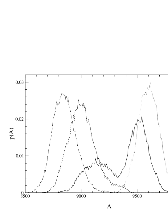
Figure 2.3: The action (energy) distribution at 4 different values of $\beta_{c}$ on the $4\times 8^{3}$ lattice for the $\xi=2$ perfect action. Dotted: $\beta=3.02$, solid: $\beta=3.03$, dashed: $\beta=3.04$, dot-dashed: $\beta=3.05$.

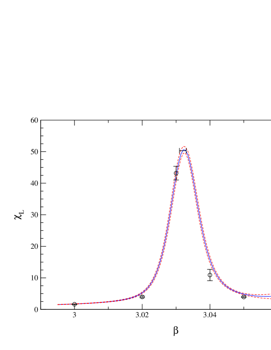
Figure 2.4: The Polyakov loop susceptibility on the $4\times 8^{3}$ lattice for the $\xi=2$ perfect action. The solid curves are the interpolations using Ferrenberg-Swendsen reweighting, the dashed lines indicate the bootstrap error.

Figure 2.5 displays the MC history of the angle of the Polyakov loop $\text{arg}(P)$ for $\beta$ close to $\beta_{c}$. It becomes apparent that most of the information about the phase (and thus about the Polyakov loop susceptibility $\chi_{P}$) is contained in the number of flips between the phases as well as in the time the configuration is staying in one of the phases. An important quantity in this respect is the persistence time $\tau_{p}$ which is the MC time (number of sweeps) divided by the number of flip-flops (change to another phase and another change back to the original phase). Because of critical slowing down, the autocorrelation time of the operators has to be considered as well. Near the phase transition knowledge about these quantities is crucial to be able to estimate the quality of the statistics given the number of sweeps performed.

Figure 2.5: MC history of the Polyakov loop measurements on a $5\times 9^{3}$ lattice at $\beta=3.12$ ($\beta_{c}$=3.118). The argument of the Polyakov loop $P$ is given, $\text{arg}(P)=0,\pm 2\pi/3$ for a configuration being in the deconfined phase.

2.3 The Static Quark-Antiquark Potential

The potential between a quark and an antiquark, both carrying colour charge, may be studied even in pure gauge theory, creating and annihilating a static quark and a static antiquark in the gauge background. As this potential is rather easy to measure and as it may be compared to experimental data obtained by studying bound states of a quark and an antiquark, the heavy mesons, it provides an excellent mean of setting the scale of lattice simulations in the absence of dynamical quarks (i.e. fermionic theories in the quenched approximation or pure Yang-Mills theory). The scale is needed if lattice results, such as masses, should be converted into physical units. In this Section, we will thus present sources of experimental data coming from light mesons in Section 2.3.1 and from heavy mesons in Section 2.3.2 as well as how the potential may be examined in pure lattice gauge theory (Sections 2.3.3, 2.3.5) and how it is used to set the scale in Section 2.3.4.

2.3.1 Light Mesons

The elementary constituents of hadronic matter, the quarks, carry colour charge which enables them to build bound states, held together by the strong force. The simplest such state consists of a quark and a corresponding antiquark. Since the early sixties it has been noticed that these states, the mesons, as well as bound states of three quarks, the baryons, having mass $m$ and spin $J$ group themselves into almost linear, so-called Regge trajectories [88, 89, 90], i.e. if one plots $m^{2}$ vs. $J$ the connection is linear. This can be observed up to spins as high as $J=11/2$. The behaviour is thus mainly

$$J(m)=\alpha(0)+\alpha^{\prime}m^{2},$$ (2.20)

where $\alpha(0)$ is known as the Regge intersect and

$$\alpha^{\prime}=\frac{1}{2\pi\sigma}$$ (2.21)

is the Regge slope with $\sigma$, the “string tension”. The explanation for this name stems from a simple model that explains the linearity of the Regge trajectories: Imagine a rotating string of length $2d$ with a constant energy density per unit length $\sigma$. If this string spans between (almost) massless quarks these quarks will move at (almost) the speed of light $c=1$ with respect to the center of mass. The velocity at a distance $r$ of the centre is thus given by $v(r)=r/d$. From this we may easily calculate the energy stored in the string,

$$m=2\int_{0}^{d}\frac{dr\sigma}{\sqrt{1-v^{2}(r)}}=\pi d\sigma,$$ (2.22)

and the angular momentum,

$$J=2\int_{0}^{d}\frac{dr\sigma rv(r)}{\sqrt{1-v^{2}(r)}}=\frac{\pi d^{2}\sigma}{2}=\frac{1}{2\pi\sigma}m^{2},$$ (2.23)

which is the relation between Regge slope and string tension in eqs. 2.20, 2.21.

The experiment predicts values of 470 MeV $<\sqrt{\sigma}<$ 480 MeV for trajectories starting with a pseudo-scalar ($\pi$ or $K$) and values around 430 MeV for the other trajectories.

2.3.2 Heavy Mesons

After the discovery of the $J/\psi$ meson consisting of a charm quark and a charm anti-quark in $e^{+}e^{-}$ annihilations it was suggested to treat such states built out of heavy quarks non-relativistically [91]. Because of the analogy to positronium in electrodynamics these states have been named quarkonia. They are composed of charm or bottom quarks, the top quark does not appear as a constituent because its weak decay rate $t\rightarrow bW^{+}$ is large (see [92]). The best studied states are $\bar{c}c$ and $\bar{b}b$, less is known about bound states of a $b$ and a $c$ quark. The string tension appearing in the Regge slope may be determined experimentally, e.g. through the mass splitting between different states of the same constituents, e.g. $1P-1S$ for $\bar{b}b$ which is $\chi_{b}-\Upsilon$. However, these measurements effectively probe a range of about 0.2 $\sim$ 1 fm where it is still difficult to extract the string tension $\sigma$ unambiguously.

For sufficiently heavy quarks the characteristic time scale of the relative movement of the quarks is much larger than the one of the gluonic degrees of freedom. In this case we may apply the adiabatic (or Born-Oppenheimer) approximation and describe the effect of gluons and sea quarks by an effective instantaneous interaction potential between the heavy quarks. In this approximation quarkonia are the positronium of QCD. However, unlike in QED, it is not possible to calculate the potential perturbatively and predict the spectrum but we have to solve the inverse problem, namely guess the form of the potential from the observed spectrum (and decay rates). The Cornell potential [93],

$$V(R)=V_{0}+\frac{\alpha}{R}+\sigma R$$ (2.24)

describes the interaction reasonably well in the energy range probed. Furthermore, there is not enough structure in the measured potential to require a more complex parametrisation. Recent results for the parameters $\alpha$ and $\sigma$ ($V_{0}$ is an unphysical constant) are $\alpha\approx-0.51$, $\sqrt{\sigma}\approx 412$ MeV [94] and $\alpha\approx-0.52$, $\sqrt{\sigma}\approx 427$ MeV [93]. However in the range 0.2 fm$<r<$ 1 fm which is probed by quarkonia splittings these parametrisations do not differ significantly even from earlier values $\alpha\approx-0.25$, $\sqrt{\sigma}\approx 455$ MeV [95] because the higher value of the Coulomb coefficient is compensated for by a smaller slope $\sigma$. Still, it is very interesting to see the compatibility of these values with the estimate for the string tension $\sigma$ from Regge trajectories of light mesons.

For an extensive review about QCD potentials and their study on the lattice see ref. [96].

2.3.3 The Static Quark-Antiquark Potential on the Lattice

In lattice gauge theory, the rectangular Wilson loop $\mathcal{W}(R,T)$, having extensions $R$ and $T$ in spatial and temporal directions respectively, starting at the point $(x,t)$, creates at time $t$ a static pair of a quark $q$ and an antiquark $\bar{q}$ sitting at $x+R$ and $x$ and annihilates it again at time $t+T$. The corresponding static potential between the colour sources is related to the expectation value of $\mathcal{W}(R,T)$ as

$$\langle\mathcal{W}(R,T)\rangle\propto\exp(-V(R)T)$$ (2.25)

for large $T$. The potential can thus be calculated in principle by

$$V(R)=\lim_{T\rightarrow\infty}-\frac{1}{T}\ln\langle\mathcal{W}(R,T)\rangle.$$ (2.26)

In pure lattice gauge theory the potential is confining the quarks and from strong coupling expansion [97, 98] it follows that the Wilson loop respects an area law

$$\langle\mathcal{W}(R,T)\rangle\propto\exp(-\sigma RT)\mbox{ for }R\rightarrow\infty,$$ (2.27)

where $\sigma$ is again the string tension between the static quark sources.

Due to the asymptotic freedom of QCD, perturbation theory is reliable at short distances. So for small $R$, it predicts a Coulomb-like interaction $V(R)\propto\alpha/R$ between the quark and the antiquark. The most simple ansatz to describe both these properties of the $q\bar{q}$-potential is the Cornell potential, eq. 2.24, mentioned in the last section. All our measurements of the Wilson loop will be fitted to this ansatz.

2.3.4 Setting the Scale Using the Static $\mathbf{q\bar{q}}$ Potential

Using the string tension $\sigma$ whose value is in principle known experimentally, one may set the scale corresponding to the coupling $\beta$ used in the simulation. However this is plagued by several problems: firstly, it is not very easy to determine the long-range quantity $\sigma$ on the lattice due to a poor signal/noise ratio for large values of $R$, the value of $\sigma$ is reached asymptotically which leads to the demand for large (and thus computationally expensive) lattices, and finally, the string tension $\sigma$ is not well defined in full QCD because if the energy of the string is large enough it may break and create a light quark-antiquark pair (“string breaking”). Due to these problems, the hadronic scale $r_{0}$ – the so-called Sommer scale – has been introduced [99] through the force $F(R)$ between the two quarks having an intermediate distance 0.2 fm $\leq r\leq 1.0$ fm. There are several advantages of the hadronic scale: Firstly, it can be measured much better on the lattice than the string tension $\sigma$, secondly, in this intermediate distance there is reliable information about the physical scale from phenomenological potential models [93, 100]. The scale is defined like

$$r_{c}^{2}F(r_{c})\equiv r_{c}^{2}\left.\frac{dV}{dR}\right|_{r_{c}}=c,$$ (2.28)

where originally $c=1.65$ has been chosen. The corresponding experimental value from bottomonium phenomenology [99, 101, 102] is $r_{0}^{-1}=(394\pm 20)$ MeV and thus $r_{0}\approx 0.50$ fm. However, it may be useful to measure the hadronic scale at different distances corresponding to other values of $c$, that is why we have collected values for $c$ and $r_{c}$ from high-precision measurements of the static potential performed with the Wilson action [103, 104, 105] listed in Table 2.1.

$r_{c}/r_{0}$	c
0.662(1)	0.89
1.00	1.65
1.65(1)	4.00
2.04(2)	6.00

Table 2.1: Parameter values for the determination of the hadronic scale through eq. 2.28.

2.3.5 Measuring the Static Potential on the Lattice

The correlation functions of the strings in MC measurements are always contaminated by high-momentum fluctuations. The common way to reduce these excited-state contaminations is smoothing the spatial links employing APE smearing (see Section 2.1.2). The Wilson loop operator $W_{nm}(R,T)$ is constructed as a product of iteratively smeared spatial links on smearing level $n$ on time slice $t$ and smearing level $m$ on time slice $t+T$ connecting two spatial points of distance $\vec{R}$ and unsmeared link products of length $T$ in temporal direction (see Figure 2.6). The Wilson loops easiest to measure are the ones parallel to the spatial axes — in this case the choice of the shortest paths is unique and the number of paths which could be taken into account and have to be measured on the lattice is small. However, taking into account separations $\vec{R}$ not parallel to the spatial axes as well has got the advantages that the discretisation of the separation $|\vec{R}|$ is not as coarse-grained, i.e. quantities like $r_{0}$ that rely on differences on the lattice can be determined more accurately and more reliably, furthermore the energies of off-axis separated quark-antiquark pairs allow to estimate effects due to violations of rotational invariance. This is why in some runs we include in the measurements separations that are multiples of the lattice vectors (1,0,0), (1,1,0), (1,1,1), (2,1,0), (2,1,1), (2,2,1) (and lattice rotations). The spatial paths are constructed such that all the shortest paths to the vectors are calculated first, out of these initial six vectors the longer separations are constructed.

Averaging the operators over the three spatial directions as well as over the whole lattice we get the zero momentum correlation matrix that can be analyzed using the variational method described in Appendix E.

Figure 2.6: The smeared Wilson loop operator $W_{nm}(R,T)$.

This method yields projectors to the ground state of the string for each $\vec{R}$ which can be used in a correlated $\chi^{2}$ fit to the phenomenological ansatz for the potential, eq. 2.24, where $R=|\vec{R}|$. The hadronic scale $r_{c}/a$ is then determined by local fits to $V(R)$ including $2\sim 4$ separations and converted to $r_{0}/a$ using Table 2.1 if necessary. Depending on the lattice spacing this can be done for several values of $c$ yielding information about systematic uncertainties.

2.4 Glueballs

2.4.1 Introduction

The particles mediating the strong interaction of QCD, the gluons, carry colour charge and thus interact with each other, unlike, e.g., their counterpart in electromagnetism, the photons, which have zero electric charge. This fact has also been established experimentally, studying 4-jet events in $e^{+}e^{-}$ annihilation. The spectrum of QCD may thus contain bound states of (mainly) gluons, called glueballs. These states are described by the quantum numbers $J$ denoting the (integral) spin, $P$ denoting the eigenvalue $\pm 1$ of the state under parity and $C$, denoting the eigenvalue $\pm 1$ under charge conjugation. Thus the eigenstates of the Hamiltonian corresponding to glueball states are labeled $|J^{PC}\rangle$.

Due to their non-perturbative nature, glueballs can be theoretically studied most reliably doing numerical simulations of QCD on a space-time lattice. As (pure) glueballs are composed entirely of glue, the study using the quenched approximation of QCD (where fermions, if present, are infinitely heavy) makes sense.

Experimentally, there is evidence for exotic glueballs or hybrid particles consisting of quarks and gluonic excitations. These states (often called “oddballs”) have exotic (or “odd”) quantum numbers (e.g., $0^{+-}$ or $1^{-+}$) and cannot be explained by simple bound states of purely quarks. Due to this, they cannot mix with mesons and are thus particularly interesting to study in pure gauge theory. However, these states are found to be high lying [106, 107, 108, 18] (above twice the mass of the lightest glueball observed). This may lead to ambiguities in the analysis of the experimental results because these states may mix with bound states of lighter particles.

The lighter glueballs with conventional quantum numbers are difficult to distinguish from the dense background of conventional meson states observed in experiments. They are expected to be created in “gluon-rich” processes, such as radiative $J/\psi$ decays, central production (two hadrons passing each other “nearly untouched” without valence quark exchange) or $\bar{p}p$-annihilation. Currently, there is an ongoing debate whether light glueballs (above all the scalar $0^{++}$ which is the lightest state in pure lattice gauge theory with a mass of about 1.6 GeV) have been observed experimentally at about the mass that is predicted by quenched simulations on the lattice, whether the lightest glueball is much lighter (below 1 GeV) and very broad[109], or whether glueballs have not been observed at all in experiments[110]. There are mainly two reasons for this uncertainty. On one hand, the experimental data seem not yet to be accurate and complete enough, despite large efforts in the last years, driven by the lattice results; on the other hand, lattice simulations with high statistics, measuring glueball states, have been performed only in the quenched approximation, where the quarks are infinitely heavy and thus static. Decreasing the sea (dynamical) quark mass (finally down to the physical value) will allow to track the glueball states as sea quark effects are increased. It may turn out, that indeed the glueball mass is lighter than the one measured in pure gauge theory (for partially quenched results possibly indicating this see [111, 112, 113]). It may even happen that by “switching on” the sea quarks the scalar glueball acquires a very large width and thus decays (almost) instantaneously to $q\bar{q}$ states, i.e. it ceases to exist physically. However, the (partially) unquenched results are rather indecisive yet.

Following the explanation that is dominant at this time, the observed low lying scalar mesons $f_{0}(1370)$, $f_{0}(1500)$ and $f_{0}(1710)$ are all mixtures of glue and mesonic components as $d\bar{d}$, $u\bar{u}$ and $s\bar{s}$. The proposed decompositions of the wave functions into these contributions [114, 115, 116, 117, 118, 119, 120, 121] are rather different, however they share some robust common features. Studies in pure gauge theory may help separating the pure gauge part from the mesonic part of these states.

2.4.2 Glueballs on the Lattice

States

Glueballs in the continuum are rotationally invariant and have a certain (integral) spin $J$. On the lattice, the rotational $O(3)$ symmetry is broken, only its discrete cubic subgroup $O_{h}$ survives the discretisation. Therefore, the eigenstates of the transfer matrix are classified according to the five irreducible representations of $O_{h}$: $A_{1}$, $A_{2}$, $E$, $T_{1}$, $T_{2}$ with dimensions 1, 1, 2, 3, 3 respectively. Their transformation properties may be described by polynomials in the components $x$, $y$, $z$ of an $O(3)$ vector as follows: $A_{1}\sim\{1\}$, $A_{2}\sim\{xyz\}$, $E\sim\{x^{2}-z^{2},y^{2}-z^{2}\}$, $T_{1}\sim\{x,y,z\}$, $T_{2}\sim\{xy,xz,yz\}$. Generally, an $O(3)$ representation with spin $J$ splits into several representations of the cubic group. Since $O_{h}$ is a subgroup of $O(3)$, any representation $D_{J}$ with spin $J$ in the continuum induces a so-called subduced representation $D_{J}\downarrow O_{h}$ on the lattice. This subduced representation no longer has to be irreducible but is a direct sum of irreducible representations $\Gamma^{p}$ of $O_{h}$:

$$D_{J}\downarrow O_{h}=\Gamma^{1}\oplus\Gamma^{2}\oplus\cdots.$$ (2.29)

Table 2.2 lists the subduced representations of $D_{J}$ for $J=1,\ldots,6$. The spin $J=2$ state for example splits up into the 2-dimensional representation $E$ and the 3-dimensional representation $T_{2}$. Approaching the continuum, rotational symmetry is expected to be restored and thus, as a consequence the mass splitting of these two states will disappear and the two representations form together the 5 states of a spin $J=2$ object.

$\Gamma^{p}$	$D_{0}$	$D_{1}$	$D_{2}$	$D_{3}$	$D_{4}$	$D_{5}$	$D_{6}$
$A_{1}$	1	0	0	0	1	0	1
$A_{2}$	0	0	0	1	0	0	1
$E$	0	0	1	0	1	1	1
$T_{1}$	0	1	0	1	1	2	1
$T_{2}$	0	0	1	1	1	1	2

Table 2.2: The composition of the subduced representation $D_{J}\downarrow O_{h}$ in terms of the irreducible representations of the cubic group $O_{h}$.

Operators

Pure glue physical states on the lattice are created and annihilated applying gauge invariant operators to the pure gauge vacuum. In our simulations, we use space-like Wilson loops in the fundamental representation of SU(3). Since we do not aim at measuring non-zero momentum glueballs we consider only translationally invariant operators, i.e. operators averaged in space.

It is computationally feasible to measure Wilson loop operators up to length 8. The composition of the irreducible representations $\Gamma^{PC}$ of the cubic group in terms of these 22 loop shapes has been done already in Ref. [122]. Figure 2.7 displays all Wilson loop shapes up to length 8 together with the numbering which will be used in the forthcoming sections. Table 2.3 lists the number of orientations of the different loop shapes. Tables 2.4, 2.5 list the irreducible contents of of the $C=+$ and $C=-$ representations of the cubic group, respectively. Certain operators contribute to the two- or three-dimensional representations with two or three different polarisations, in analogy to different magnetic quantum numbers $m$ for a given angular momentum $l$ in the O(3) group. Measuring all these polarisations may suppress statistical noise more than just increasing statistics since the different polarisations of a loop shape are expected to be anti-correlated. Examining the measured correlators of different polarisations of the same representation, it turns out that in most cases one of the polarisations is measured very well, whereas the others exhibit a bad signal/noise ratio.

Figure 2.7: All space-like Wilson loop shapes up to length 8.

loop shape #	1	2	3	4	5	6	7	8	9	10	11
dimension $d$	6	12	24	8	6	24	24	96	48	12	48
loop shape #	12	13	14	15	16	17	18	19	20	21	22
dimension $d$	24	12	24	6	12	12	48	12	48	24	96

Table 2.3: Dimension $d$ of the representation of $O_{h}\times C$ on the loop shapes, i.e. number of different orientations.

loop	$A_{1}^{++}$	$A_{2}^{++}$	$E^{++}$	$T_{1}^{++}$	$T_{2}^{++}$	$A_{1}^{-+}$	$A_{2}^{-+}$	$E^{-+}$	$T_{1}^{-+}$	$T_{2}^{-+}$
#1	1	0	1	0	0	0	0	0	0	0
#2	1	1	2	0	0	0	0	0	0	0
#3	1	0	1	0	1	0	0	0	1	1
#4	1	0	0	0	1	0	0	0	0	0
#5	1	0	1	0	0	0	0	0	0	0
#6	1	0	1	0	1	0	0	0	1	1
#7	1	0	1	0	1	0	0	0	1	1
#8	1	1	2	3	3	1	1	2	3	3
#9	1	0	1	1	2	1	0	1	1	2
#10	1	1	2	0	0	0	0	0	0	0
#11	1	1	2	1	1	0	0	0	2	2
#12	1	1	2	1	1	0	0	0	0	0
#13	1	0	1	0	0	0	0	0	0	1
#14	1	0	1	1	2	0	0	0	0	0
#15	1	0	1	0	0	0	0	0	0	0
#16	1	1	2	0	0	0	0	0	0	0
#17	1	0	1	0	1	0	0	0	0	0
#18	1	0	1	1	2	1	0	1	1	2
#19	1	0	1	0	1	0	0	0	0	0
#20	1	0	1	1	2	1	0	1	1	2
#21	1	0	1	0	1	0	0	0	1	1
#22	1	1	2	3	3	1	1	2	3	3

Table 2.4: Irreducible contents of the $C$-parity plus representations of the symmetry group of the cube on Wilson loops up to length eight.

loop	$A_{1}^{+-}$	$A_{2}^{+-}$	$E^{+-}$	$T_{1}^{+-}$	$T_{2}^{+-}$	$A_{1}^{--}$	$A_{2}^{--}$	$E^{--}$	$T_{1}^{--}$	$T_{2}^{--}$
#1	0	0	0	1	0	0	0	0	0	0
#2	0	0	0	1	1	0	0	0	0	0
#3	0	0	0	1	1	1	0	1	0	1
#4	0	1	0	1	0	0	0	0	0	0
#5	0	0	0	1	0	0	0	0	0	0
#6	0	0	0	1	1	1	0	1	0	1
#7	0	1	1	1	0	0	0	0	1	1
#8	1	1	2	3	3	1	1	2	3	3
#9	0	1	1	2	1	0	1	1	2	1
#10	0	0	0	1	1	0	0	0	0	0
#11	0	0	0	2	2	1	1	2	1	1
#12	0	0	0	2	2	0	0	0	0	0
#13	0	0	0	1	0	0	1	1	0	0
#14	0	1	1	2	1	0	0	0	0	0
#15	0	0	0	1	0	0	0	0	0	0
#16	0	0	0	0	0	0	0	0	1	1
#17	0	0	0	0	0	0	0	0	1	1
#18	0	1	1	2	1	0	1	1	2	1
#19	0	1	1	1	0	0	0	0	0	0
#20	1	0	1	1	2	1	0	1	1	2
#21	0	0	0	1	1	0	1	1	1	0
#22	1	1	2	3	3	1	1	2	3	3

Table 2.5: Irreducible contents of the $C$-parity minus representations of the symmetry group of the cube on Wilson loops up to length eight.

The accuracy of the measurements of different operators may differ considerably; firstly, because shapes with larger multiplicity show smaller statistical noise, secondly, because operators on different smearing schemes may exhibit less or more fluctuations. To give an impression of the differences between various operators, Tables 2.6, 2.7 display correlator “lifetimes” obtained from the glueball measurements at coupling $\beta=3.3$, with a temporal lattice spacing $a_{t}\approx 0.08$ fm $\approx$ (2.4 GeV)^-1. The correlator lifetime $\tau_{\text{corr}}$ is (conventionally) defined such that at time $t=\tau_{\text{corr}}$ the relative (bootstrap) error of the correlator is 25%. The relative error is linearly interpolated between $t<\tau_{\text{corr}}$ and $t+1>\tau_{\text{corr}}$. Table 2.6 compares the shapes contributing to different glueball representations, measured on smearing level 1 (3 times smeared) at $\beta=3.3$, Table 2.7 compares the same quantities measured on smearing level 3 (9 times smeared). For shapes which contribute with more than one projection to a given representation, the best measured projection is displayed — usually the other polarisations are measured much worse due to the anti-correlation.

The operators measured on different smearing levels are again used in the variational method described in Appendix E. The scalar representation $A_{1}^{++}$ picks up a vacuum expectation value due to having the same quantum numbers as the vacuum. The standard procedure is to measure these vacuum expectation values and subtract them from the correlation matrix elements as

$$C_{ij}(t)=\frac{1}{N_{t}}\sum_{\tau}\langle O_{i}(\tau)O_{j}(\tau+t)\rangle-\langle O_{i}\rangle\langle O_{j}\rangle,$$ (2.30)

however during the analysis of our measurements, it turns out to be better to treat the vacuum on the same footing as the other states in the vacuum channel, i.e. as a state having mass 0. We thus just cut out the vacuum state obtained from solving the initial generalised eigenvalue problem (see Appendix E) and perform the fit on the remaining states.

loop	$A_{1}^{++}$	$A_{2}^{++}$	$E^{++}$	$T_{1}^{++}$	$T_{2}^{++}$	$A_{1}^{-+}$	$E^{-+}$	$T_{2}^{-+}$	$A_{2}^{+-}$	$T_{1}^{+-}$	$T_{2}^{+-}$
#1	4.0		2.2							1.2
#2	4.2	2.0	2.7							1.7	1.1
#3	4.0		2.3		4.0			2.1		1.6	1.5
#4	5.0				4.0				1.4	1.6
#5	5.0		3.4							2.1
#6	4.4		3.0		4.1			2.1		2.1	2.1
#7	4.6		3.1		2.1			1.0	1.3	2.0
#8	4.2	2.0	3.0	2.0	4.1	3.0	2.2	2.2	0.6	2.0	2.0
#9	4.0		1.4	1.8	4.1	2.9	2.1	2.2	1.9	2.0	1.2
#10	4.5	2.1	3.1							1.8	1.4
#11	4.2	1.9	2.8	2.0	4.2			2.2		1.8	1.4
#12	4.2	1.9	3.0	2.0	4.1					2.0	1.6
#13	3.9		2.4					2.0		1.5
#14	4.5		2.8	2.0	4.2				1.5	2.1	2.1
#15	4.0		2.3							1.3
#16	3.0	2.0	1.9
#17	3.0		2.0		3.0
#18	3.9		2.2	1.5	3.6	2.9	2.1	2.4	1.0	1.7	1.9
#19	4.2		2.8		2.0				1.1	1.9
#20	4.0		2.3	1.5	3.6	2.9	2.2	2.4		2.0	1.5
#21	3.8		2.1		4.0			2.1		1.6	1.6
#22	4.2	2.0	3.1	2.0	4.2	3.0	2.2	2.6	1.6	2.0	2.0

Table 2.6: “Lifetimes” of glueball correlators at $\beta=3.5$ (first smearing scheme, 3 times smeared); see text.

loop	$A_{1}^{++}$	$A_{2}^{++}$	$E^{++}$	$T_{1}^{++}$	$T_{2}^{++}$	$A_{1}^{-+}$	$E^{-+}$	$T_{2}^{-+}$	$A_{2}^{+-}$	$T_{1}^{+-}$	$T_{2}^{+-}$
#1	6.0		4.8							0
#2	6.1	1.4	5.1							2.4	0
#3	6.0		4.9		5.9			3.9		1.8	0.4
#4	6.0				5.9				0.2	1.8
#5	6.3		5.2							3.0
#6	6.2		5.2		6.1			4.1		3.0	3.1
#7	6.2		5.1		3.1			0	0.2	3.0
#8	6.1	3.0	5.1	2.4	6.1	4.2	3.4	4.0	0	3.0	2.6
#9	6.0		2.3	2.4	6.1	4.2	3.4	4.0	1.1	3.0	0.2
#10	6.2	3.1	5.2							3.1	1.3
#11	6.1	2.7	5.1	2.6	6.0			4.0		3.0	2.1
#12	6.1	2.0	5.1	2.3	6.1					3.0	1.6
#13	5.9		4.9					3.9		0.6
#14	6.2		5.2	2.6	6.1				2.2	3.0	2.7
#15	6.0		4.8							2.2
#16	5.1	1.4	2.2
#17	5.1		2.6		3.1
#18	5.9		4.7	2.5	6.1	4.2	3.4	4.0	0	2.1	0.7
#19	6.2		5.1		3.1				0	2.3
#20	6.0		5.0	2.5	6.1	4.2	3.4	4.0		2.2	0.7
#21	5.9		4.7		5.9			3.9		1.6	0.4
#22	6.1	3.0	5.1	2.6	6.1	4.2	3.5	4.0	2.3	3.0	2.2

Table 2.7: “Lifetimes” of glueball correlators at $\beta=3.5$ (third smearing scheme, 9 times smeared); see text.

Why Anisotropic Lattices?

Due to the rather high mass of glueball states and large vacuum fluctuations of the operators the signal to noise ratio decreases very rapidly as the temporal separation of the source and the sink is increased. This demands a small lattice spacing such that the signal can be traced over several slices increasing the computational cost drastically because the physical volume still has to be kept large enough ($La\gtrsim 1.2$ fm) in order to avoid severe finite-volume effects.

The common way to ensure good resolution of the signal on a lattice of moderate size is using anisotropic lattices.

The history of glueball measurements on the lattice employing anisotropic gauge actions is not very long, despite this the most reliable results from pure gluodynamics stem from anisotropic simulations. The first study, using a tree-level and tadpole improved action has been performed by Morningstar and Peardon in 1996 [123]. This was followed by additional studies of the same group [108, 124, 18, 19]. In 1997, the Kentucky Glueball Collaboration studied glueball matrix elements on anisotropic lattices [125]. A recent study of the glueball spectrum, using the same action as Morningstar and Peardon, has been performed by Liu [20, 126].

Chapter 3 Recapitulation: Properties of the Isotropic Action

As the anisotropic perfect action is based on the isotropic FP action parametrised using “fat” links it is useful to recapitulate briefly the properties and the results of measurements of physical quantities with the isotropic action [1, 2, 3].

The measurements that have been performed using the isotropic action comprise the critical temperature $T_{c}$ of the deconfining phase transition, the static quark-antiquark potential as well as the lower lying part of the glueball spectrum. These quantities and techniques used to measure them are presented in detail in Chapter 2.

This Chapter is organised as follows: In Section 3.1 the action is presented, Section 3.2 contains results about the deconfining phase transition, in Section 3.3 the results about the static $q\bar{q}$ potential are summarised, in Section 3.4 we report about scaling tests of the FP action, and finally, in Section 3.5 we present the results about glueball spectroscopy. For additional information, such as run parameters and more detailed results, consult [1, 2].

3.1 The Isotropic Action

The isotropic FP action has been constructed using the block transformation introduced in [60] (see Section 4.2) which has been optimised for a short interaction range of the FP action as well as for improved rotational invariance compared to the standard Swendsen-blocking which uses long staples.

The action has been parametrised using the parametrisation presented in Section 4.3.1, where the non-linear parameters $\eta$, $c_{i}$ have been chosen to be constant (no $x_{\mu}(n)$-dependence), $i=1$, 2, 3 and the linear parameters $p_{kl}$ in the mixed polynomial of the standard and smeared staples $u$, $w$ are non-zero for $0<k+l\leq 4$. The values of the parameters are given in Appendix D.1.

3.2 The Deconfining Phase Transition

The properties of the deconfining phase transition in pure Yang-Mills theory are described in Section 2.2. On the isotropic lattice we have measured the critical couplings $\beta_{c}$ corresponding to temporal extensions $N_{t}=2,3,4$ of the lattice.

3.2.1 Details of the Simulations Performed

To determine the susceptibility $\chi$, we measure, in the equilibrated system, the Polyakov loops averaged over the lattice

$$P\equiv\frac{1}{N_{s}^{3}}\sum_{\vec{x}}P(\vec{x}),$$ (3.1)

where $P(\vec{x})$ is defined in eq. 2.9, as well as the action values of the corresponding configurations. The measurement is performed after each sweep of updates as it is computationally inexpensive. Both values are stored for later use in the spectral-density reweighting procedure, described in Section 2.2.1

We have performed a large number of simulations on lattices with temporal extensions $N_{t}=$ 2, 3, 4 at 3 to 6 different $\beta$ values near the estimated critical couplings $\beta_{c}(N_{t})$. Additionally, various spatial extensions $N_{s}/N_{t}=2.5\ldots 5$ have been explored in order to be able to examine the finite size scaling of $\beta_{c}$. The configurations have been generated by alternating Metropolis and pseudo-over-relaxation steps (see Sections 8.1.1, 8.1.2).

The critical coupling, i.e. the location of the peak of the susceptibility, is determined employing the spectral density reweighting method which allows to calculate observables away from the actual $\beta$ values at which the simulations have been performed [127, 128, 87, 86] (see Section 2.2.1).

To get the value of $\beta_{c}$ for infinite spatial volume we use the finite-size scaling law for first order phase transitions:

$$\beta_{c}(N_{t},N_{s})=\beta_{c}(N_{t},\infty)-h\left(\frac{N_{t}}{N_{s}}\right)^{3},$$ (3.2)

where $h$ denotes a universal quantity in principle independent of $N_{t}$.

3.2.2 Results

In Table 3.1 we display the values of $\beta_{c}(V_{s})$ together with the infinite volume extrapolations according to Eq. 3.2. Studying the deconfining phase transition provides accurate information about the scale at couplings $\beta_{c}$. This has been used in scaling tests (see Section 3.4) where the critical temperature $T_{c}\propto 1/a$ is compared to the hadronic scale $r_{0}\propto a$ whose determination for the isotropic action is described in the following Section.

$N_{s}$	$\beta_{c}(N_{t}=2)$	$\beta_{c}(N_{t}=3)$	$\beta_{c}(N_{t}=4)$
6	2.3552(24)
8	2.3585(12)	2.6826(23)
10	2.3593(7)	2.6816(12)	2.9119(31)
12		2.6803(10)	2.9173(20)
14			2.9222(20)
$\infty$	2.3606(13)	2.6796(18)	2.9273(35)
$h$	0.14(9)	-0.05(7)	0.25(9)

Table 3.1: Results of the critical couplings $\beta_{c}$ from the peak location of the Polyakov loop susceptibility and the corresponding infinite volume limit obtained according to eq. 3.2. The finite size scaling constant $h$ is also given.

3.3 The Static Quark-Antiquark Potential

The static quark-antiquark potential as described in Section 2.3 is used to set the scale of our simulations (determining the lattice spacing $a$) as well as to examine the scaling properties of the FP action, i.e. measuring lattice artifacts.

3.3.1 Details of the Simulation

Simulations with the isotropic FP action including measurements of the static quark-antiquark potential have been performed at six different values of $\beta$, three of them corresponding to the critical couplings indicated in Section 3.2. The updates have been performed using alternating Metropolis and pseudo-over-relaxation sweeps. Based on earlier observations in [103, 104, 129] the spatial extent of the lattice has always been chosen to be at least (1.5 fm)³.

The measurements have been performed as described in Section 2.3.5, for measuring the potential we have chosen $\lambda_{s}=0.2$ in the APE smearing of the operators (see Section 2.1.2) and used smearing levels $n=$ 0, 1, 2, 3, 4.

3.3.2 Results

It turns out that on coarse lattices with $a_{s}\gtrsim 0.15$ fm systematic ambiguities occur determining $r_{0}$ on different fitting ranges or using different (reasonably chosen) values of $c$, see Section 2.3.4. The main reason for this is the difficulty emerging to define the derivative $dV/dR$ having at hand discrete values of $R$. Estimates for these systematic ambiguities are displayed together with the results for $r_{0}/a$ in Table 3.2. A possible solution to this problem is including off-axis separations of the quark and the anti-quark which makes the measurements rather expensive. However, violations of rotational symmetry show up in this case and allow the estimation of systematic errors in $r_{0}$ if the result is changed beyond statistical uncertainty.

$\beta$	$N_{\tau}$	2cm$r_{0}/a$
3.400		$4.833(39)(\genfrac{}{}{0.0pt}{}{+18}{-22})$
3.150		$3.717(23)(\genfrac{}{}{0.0pt}{}{+16}{-17})$
2.927	4	$2.969(14)(\genfrac{}{}{0.0pt}{}{+5}{-14})$
2.860		$2.740(10)(\genfrac{}{}{0.0pt}{}{+17}{-31})$
2.680	3	$2.237(7)(\genfrac{}{}{0.0pt}{}{+11}{-33})$
2.361	2	$1.500(5)(\genfrac{}{}{0.0pt}{}{+29}{-14})$

Table 3.2: The hadronic scale $r_{0}/a$ determined from local fits to the potential. The first error denotes the statistical error and the second is the estimate of systematic ambiguities (see text).

The full static $q\bar{q}$ potentials $aV(R)$ measured on lattices with different $\beta$, i.e. different lattice spacings $a$, may be compared directly if $V(R)$ is measured in terms of $r_{0}$ and the unphysical constant $r_{0}V_{0}$ is eliminated by subtracting e.g. $r_{0}V(r_{0})$ for each lattice spacing. This yields Figure 3.1 and it turns out that all the measurements agree excellently. Also, the result of [130], represented by the dotted line, is hardly distinguishable from our measurements.

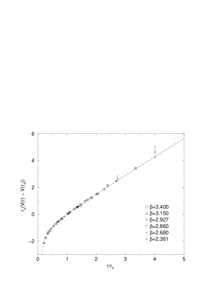
Figure 3.1: The static quark-antiquark potential $V(R)$ expressed in terms of the hadronic scale $r_{0}$. To match the curves at $r=r_{0}$ the unphysical constant $r_{0}V(r_{0})$ is subtracted for each value of $\beta$. The dashed line is a fit of all the data to the Cornell potential, eq. 2.24, the dotted line stems from ref. [130].

3.3.3 The Interpolating Formula

The information about the scale obtained in the potential measurements may be nicely collected in an (ad-hoc) interpolating formula that connects the bare coupling $\beta$ to the lattice spacing (in units of the hadronic scale $r_{0}$) $a/r_{0}$. Our fit (analogous to the ones in [104, 105]) yields

$$\ln(a/r_{0})=-1.1622(24)-1.0848(95)(\beta-3)+0.156(17)(\beta-3)^{2}$$ (3.3)

which describes very well the data points in the range $2.361\leq\beta\leq 3.4$.

3.4 Scaling Properties

The parametrised FP action is assumed to reduce lattice artifacts considerably. In order to check this assumption one may study the scaling properties of renormalisation group invariant quantities, measuring them on lattices of different lattice spacings. Dimensionless ratios or products of physical quantities which are RG invariant are constant if there are no scaling violations (due to lattice artifacts), it is therefore very convenient to study such observables.

Having at hand the physical quantities $r_{0}$, the hadronic scale, and $\sigma$, the string tension, from the potential measurements as well as the critical temperature $T_{c}$ from the study of the deconfining phase transition, we may build up the dimensionless combinations $T_{c}/\sqrt{\sigma}$, $r_{0}T_{c}$ and $r_{0}\sqrt{\sigma}$.

In this section we present the results for the FP action and compare them to results obtained for the Wilson action and different other improved actions as far as they are available.

3.4.1 $\mathbf{T_{c}/\sqrt{\sigma}}$

The results for $T_{c}/\sqrt{\sigma}$, the critical temperature of the deconfining phase transition in terms of the string tension, measured on lattices of different $\beta$ are compared to the continuum extrapolations for other gauge actions in Table 3.3. The Wilson action data stem from [131] where results from [132] have been used. From the same reference we state the value for the $1\times 2$ tree-level improved action. “DBW2” stands for “doubly blocked from Wilson in two coupling space”, the results of this action stem from [133]. Iwasaki [134] has performed measurements with the RG improved (Iwasaki) action [135]. Finally, the results obtained using a tree level and tadpole improved action are from [136]. The continuum extrapolations for all these different actions stem from a systematic reanalysis [137] of the data.

action	$\beta$	$T_{c}/\sqrt{\sigma}$
FP action	2.927	0.624(7)
	2.680	0.622(8)
	2.361	0.628(11)
Wilson [131]	$\infty$	0.630(5)
$1\times 2$ tree-level improved [131]	$\infty$	0.634(8)
DBW2 [133]	$\infty$	0.627(12)
RG improved [134]	$\infty$	0.651(12)
tree-level/tadpole improved [136]	$\infty$	0.659(8)

Table 3.3: Results of the deconfining temperature in units of the string tension obtained with the FP action and continuum values for different other actions.

These values, together with those for finite lattice spacings, are displayed in Figure 3.2. Our measurements are all compatible with the continuum extrapolation of the Wilson data and we observe no scaling violations of the FP action within statistical errors even on very coarse lattices corresponding to $N_{t}$=2. The continuum results obtained using the RG improved action as well as the tree-level and tadpole improved action lying considerably higher (about $3\sigma$ for the latter) may be explained by ambiguities occurring with the measurement of the string tension $\sigma$. Depending on the separations $r$ of the static quarks taken into account performing the fit to the Cornell potential, eq. 2.24, the obtained value of the string tension may vary considerably (together with variations of the Coulomb parameter $\alpha$), such that determinations by different groups may differ systematically if the methods do not coincide. Especially, Bliss et al. [136], having studied the treelevel and tadpole improved action, determined the string tension $\sigma$ using results coming from torelon measurements and employing the string formula, eq. 2.1.

Figure 3.2: The dimensionless quantity $T_{c}/\sqrt{\sigma}$ vs. $1/N_{t}^{2}$ for different actions.

3.4.2 $\mathbf{r_{0}T_{c}}$

Whereas it was easy to find data for the quantity $T_{c}/\sqrt{\sigma}$ presented in the last section, precise determinations of $r_{0}/a$ are missing in the literature except for the Wilson action [104, 105] and thus we are not able to compare our results for $r_{0}T_{c}$ to a large number of other actions. Our results compared to those obtained with the Wilson action are displayed in Table 3.4. The Wilson results for the critical couplings $\beta_{c}(N_{t})$, $N_{t}=$ 4, 6, 8, 12 have been taken from [131] and the corresponding values of $r_{0}/a$ have been calculated using the interpolating formula from [105]. The continuum value has been extrapolated using a linear fit in the leading correction term $1/N_{t}^{2}$ on $N_{t}=$ 4, 6, 8. Figure 3.3 displays the same quantities; including the systematic ambiguities on coarse lattices (dashed lines), see Section 3.3.2.

$N_{\tau}$	Wilson action	FP action
2		0.750(3)
3		0.746(3)
4	0.719(2)	0.742(4)
6	0.739(3)
8	0.745(3)
12	0.746(4)
$\infty$	0.750(5)

Table 3.4: Results for the critical temperature in terms of the hadronic scale, $r_{0}T_{c}$, from measurements with the Wilson action [131, 105], and the FP action.

Figure 3.3: The dimensionless quantity $r_{0}T_{c}$ vs. $1/N_{t}^{2}$ for the FP action compared to the Wilson action [131, 105], the dashed error bars indicate the systematic error from ambiguities in calculating the force $F(R)=V^{\prime}(R)$ on coarse lattices.

Compared to the Wilson action, which shows scaling violation of about 4 % at $N_{t}=4$ the FP action performs much better in this scaling test exhibiting scaling within 1 % even on very coarse lattices corresponding to $N_{t}=3$ and 2. However this statement is softened due to the large systematic uncertainties at larger lattice spacings.

3.4.3 $\mathbf{r_{0}\sqrt{\sigma}}$

The dimensionless product $r_{0}\sqrt{\sigma}$ contains two (physical) quantities obtained in the fit of the static quark-antiquark potential. However its scaling properties are not trivial as $r_{0}$ probes the intermediate range and $\sigma$ the long range properties of the potential. We are thus using the values of $r_{0}/a$ obtained from local fits to the potential (Table 3.2) , whereas the values of $\sigma a^{2}$ are determined from global fits including large values of $R$. Table 3.5 collects the resulting values of $r_{0}\sqrt{\sigma}$ together with results from the Wilson action calculated using the interpolating formula for $r_{0}/a$ from [105] and the parametrisation for the string tension from [104]. The continuum extrapolation of the Wilson data has been performed in [137]. The same data is displayed in Figure 3.4. The error bars are purely statistical and dominated by the errors of the string tension — the systematic ambiguities in $r_{0}$ may thus be neglected in this case.

Wilson action		FP action
$\beta$	$r_{0}\sqrt{\sigma}$	$\beta$	$r_{0}\sqrt{\sigma}$
5.6925	1.148(12)	2.361	1.194(21)
5.8941	1.170(19)	2.680	1.196(15)
6.0624	1.183(13)	2.860	1.190(23)
6.3380	1.185(11)	2.927	1.191(12)
		3.150	1.185(16)
		3.400	1.198(12)
$\infty$	1.197(11)	$\infty$	1.193(10)

Table 3.5: $r_{0}\sqrt{\sigma}$ for the Wilson [105, 104, 137] and the FP action.

Figure 3.4: Scaling behaviour of $r_{0}\sqrt{\sigma}$ for the Wilson action [105, 104, 137] (empty circles) and the FP action (filled squares).

Again, the Wilson action shows scaling violations of about 4 % for $N_{t}=4$ whereas the FP action exhibits no artifacts even on lattices as coarse as $\beta=2.361$ (corresponding to criticality for $N_{t}=2$).

3.5 Glueball Spectroscopy

The physical nature of glueballs and how they can be studied on the lattice is described in Section 2.4. Numerical simulations using the methods described there have been performed using the isotropic FP action and will be described in this Section.

3.5.1 Details of the Simulation

The simulations have been performed on three different lattice spacings in the range 0.10 fm $\leq a\leq$ 0.18 fm and volumes between (1.4 fm)³ and (1.8 fm)³. The updates have been performed using alternating Metropolis and pseudo-over-relaxation sweeps (see Sections 8.1.1, 8.1.2). For the listing of all the simulation parameters see Table 3.6.

$\beta$	lattice	$r_{0}/a$	$a$ [fm]	# sweeps / measurements
2.86	$10^{4}$	2.740(10)	0.18	32000 / 8000
3.15	$12^{4}$	3.717(23)	0.13	101000 / 10100
3.40	$14^{4}$	4.833(39)	0.10	86520 / 14420

Table 3.6: Run parameters for the glueball measurements using the isotropic FP action.

In the first simulation, performed on a coarse lattice with $\beta=2.86$, only the mass of the lowest-lying $A_{1}^{++}$ channel has been determined measuring the loop shapes 2, 4, 7, 10, 18 (see Figure 2.7) which had been shown to be measured well and having a large overlap with the state in a short pilot run. For the other two simulations all 22 Wilson loop shapes up to length 8 are measured and projected to all 20 irreducible glueball representations. To kill ultraviolet fluctuations and to enhance the overlap with the glueball states the measurements are performed on five smearing levels ${\cal S}_{n}U$, $n=2,4,\ldots,10$ with smearing parameter $\lambda_{s}=0.2$ (see Section 2.1.2).

It turns out that there are operators which are measured notoriously bad, i.e. that have a small signal/noise ratio. As there are representations with contributions of as many as 145 operators (the representation $T_{1}^{+-}$ on five smearing levels) this may destabilise the fitting procedure described in Appendix E. That is why we remove badly measured operators right from the start of the analysis.

For the scalar glueball, the vacuum expectation values are not subtracted from the operators, but the vacuum state is treated like the other states in the vacuum channel, see Section 2.4.2.

3.5.2 Results

The full (and rather lengthy) lists of results are contained in [2], we only display the masses of the lowest-lying and best measured states in units of the hadronic scale $r_{0}$ compared to the results of other groups in Tables 3.7, 3.8. The results denoted by UKQCD, Teper and GF11 have been obtained using the Wilson action whereas the results of Morningstar and Peardon (M&P) and Liu have been measured using a tree-level/tadpole improved anisotropic action.

Collab.	$r_{0}m_{0^{++}}$	$r_{0}m_{2^{++}}$	year
UKQCD [107]	4.05(16)	5.84(18)	1993
Teper [137]	4.35(11)	6.18(21)	1998
GF11 [138]	4.33(10)	6.04(18)	1999
M&P [18]	4.21(15)	5.85(8)	1999
Liu [20]	4.23(22)	5.85(23)	2000
FP action	4.12(21)	[5.96(24)]	2000

Table 3.7: Comparison of the two lowest glueball masses in units of $r_{0}$. Our $2^{++}$ value is not extrapolated to the continuum but is the mass obtained at a lattice spacing $a=0.10$ fm.

Collab.	$r_{0}m_{0^{-+}}$	$r_{0}m_{2^{-+}}$	$r_{0}m_{1^{+-}}$	year
Teper [137]	5.94(68)	8.42(78)	7.84(62)	1998
M&P [18]	6.33(13)	7.55(11)	7.18(11)	1999
FP action	[6.74(42)]	[8.00(35)]	[7.93(78)]	2000

Table 3.8: Comparison of glueball masses in units of $r_{0}$. Values in brackets denote masses obtained at a lattice spacing $a=0.10$ fm and are not extrapolated to the continuum.

The results for the scalar ($0^{++}$) glueball are displayed together with the ones of other groups in Figure 3.5, the results for the $2^{++}$ glueball which is composed of the two representations $E^{++}$ and $T_{2}^{++}$ in Figure 3.6.

Figure 3.5: Mass estimates for the $0^{++}$ glueball. Results from simulations of the Wilson action (crosses) and a tree level/tadpole improved anisotropic action (empty circles) are shown together with the results obtained with the FP action (filled circles).

Figure 3.6: Mass estimates for the $2^{++}$ glueball. Results from simulations of the Wilson action (crosses) and a tree level/tadpole improved anisotropic action (empty symbols) are shown together with the results obtained with the FP action (filled symbols). Squares and circles denote the $E^{++}$ and $T_{2}^{++}$ mass estimates, respectively.

Chapter 4 The Construction of Perfect Anisotropic Actions

In this Chapter we describe our concept of generating anisotropic perfect actions without having to repeat the whole lengthy procedure described in Section 1.4, making use of the parametrisation of the isotropic FP action [1, 2, 3]. In Section 4.1 we describe two methods one might think of, in the following we concentrate on the one of the two ways which is presented more deeply in Section 4.2. The parametrisation ansatz, for the isotropic as well as for the anisotropic case is finally presented in Section 4.3.

4.1 Methods

The method for constructing FP actions (see Section 1.3.2) may be straightforwardly generalised to anisotropic lattices in two different ways, illustrated, together with the isotropic method, in Figure 4.1: Firstly, one might repeat the procedure used to generate the isotropic FP action (see Section 1.4), starting with an anisotropic action $\mathcal{A}_{0}^{\text{ai}}$ which behaves well on very small fluctuations and doing the same cascade process involving blocking steps and parametrisations as before. Of course, the parametrisation has to be adapted such that it may account for the space/time asymmetry.

Secondly, one may start with an isotropic parametrised FP action on rather large fluctuations (e.g. with the action $\mathcal{A}_{5}^{444}$, see Appendix D) and perform a small number of purely spatial blocking steps. If a scale 2 block transformation is used, the resulting actions will have anisotropies $\xi=$ 2, 4, 8, $\ldots$. This second approach may be performed much faster than the first one because the number of minimisation/fitting steps is smaller and one does not have to construct and check a new (anisotropic) starting action $\mathcal{A}_{0}^{\text{ai}}$. It is because of this we concentrate in this work on the spatial blocking approach described in the next section.

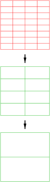
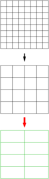
Figure 4.1: Different methods of creating a FP action. left: isotropic action; center: anisotropic action, using an anisotropic starting action; right: anisotropic action, performing purely spatial blocking steps in the end.

4.2 Spatial Blocking

To perform the blocking only spatially, doubling the lattice spacing in spatial direction while leaving the temporal lattice spacing unchanged, we modify the blocking kernel $T(U,V)$ of the symmetric RGT 3 transformation [60], appearing in eq. 1.5

$$T(U,V)=\sum_{n_{B},\mu}\left(\mathcal{N}_{\mu}^{\infty}(n_{B})-\frac{\kappa}{N}\text{Re Tr}[V_{\mu}(n_{B})Q_{\mu}^{\dagger}(n_{B})]\right),$$ (4.1)

with the normalisation

$$\mathcal{N}_{\mu}^{\infty}(n_{B})=\max_{W\in\text{SU(N)}}\left\{\frac{\kappa}{N}\text{Re Tr}[WQ_{\mu}^{\dagger}(n_{B})]\right\}$$ (4.2)

and the blocked link

$$Q_{\mu}(n_{B})=W_{\mu}(2n_{B})W_{\mu}(2n_{B}+\hat{\mu}),$$ (4.3)

where $W_{\mu}(n)$ denotes a smeared (fuzzy) fine link, which is constructed as follows. In addition to the simple staples we build as well diagonal staples by first going in the planar or spatial diagonal directions orthogonal to the direction $\mu$ of the final smeared link, then doing a step in direction $\mu$ and finally returning along the corresponding diagonal to $n+\hat{\mu}$. To be specific, let us first build matrices $W^{(m)}(n,n^{\prime})$ connecting the sites $n$ and $n^{\prime}$ where $n^{\prime}$ is a neighbouring site orthogonal to the smeared link $W_{\mu}(n)$ to be built:

$$W^{(0)}(n,n)=1\,,$$ (4.4a)

$$W^{(1)}(n,n+\hat{\nu})=U_{\nu}(n)\,,$$ (4.4b)

$$W^{(2)}(n,n+\hat{\nu}+\hat{\rho})=\frac{1}{2}\left(U_{\nu}(n)U_{\rho}(n+\hat{\nu})+U_{\rho}(n)U_{\nu}(n+\hat{\rho})\right)\,,$$ (4.4c)

$$W^{(3)}(n,n+\hat{\nu}+\hat{\rho}+\hat{\lambda})=\frac{1}{6}\left(U_{\nu}(n)U_{\rho}(n+\hat{\nu})U_{\lambda}(n+\hat{\nu}+\hat{\rho})+\mbox{perms.}\right)\,.$$

(4.4d)

Here $\nu$, $\rho$ and $\lambda$ go over all (positive and negative) directions different from $\mu$ and from each other. In eqs. 4.4c, 4.4d the sum is taken over all shortest paths leading to the endpoint $n^{\prime}$ of the corresponding diagonal. The fuzzy link operator $W_{\mu}(n)$ is then constructed by a modified Swendsen smearing [139, 140, 141, 142, 143]:

$$W_{\mu}(n)=\sum_{m=0}^{3}\sum_{n^{\prime}}c_{m}W^{(m)}(n,n^{\prime})U_{\mu}(n^{\prime})W^{(m)}(n^{\prime}+\hat{\mu},n+\hat{\mu}).$$ (4.5)

The coefficients $c_{m}$ are free parameters subject to the constraint:

$$c_{0}+6\,c_{1}+12\,c_{2}+8\,c_{3}=1.$$ (4.6)

This normalisation condition ensures that for a trivial field configuration, $W_{\mu}(n)$ is equal to the unit matrix. These parameters $c_{m}$ have been optimised for a short ranged quadratic FP action [60] and take on the values $c_{1}$=0.07, $c_{2}$=0.016, $c_{3}$=0.008 and thus $c_{0}$=0.324.

To modify the isotropic definition, in order to end up with a purely spatial blocking, we set

$$Q_{4}(n_{B})=W_{4}(2n_{B})$$ (4.7)

thus doing only a smearing and no blocking in temporal direction. (In the case of spatial blocking the expression “$2n_{B}$” stands for $(2n_{B}^{1},2n_{B}^{2},2n_{B}^{3},n_{B}^{4})$.) Additionally, we have the freedom to choose different values of $\kappa$ for spatial ($\kappa_{s}$) and temporal ($\kappa_{t}$) links (see also Appendix A).

4.3 The Parametrisation

As already stated, the FP-type actions, described in principle by an infinite number of couplings, have to be parametrised in order to be useful for numerical simulations. We have shown that a parametrisation of the isotropic FP gauge action including APE-like smearing behaves much better and is much more flexible compared to common parametrisations using traces of closed loops with comparable computational cost [1, 2, 3]. Thus the starting point for the parametrisation of the anisotropic perfect gauge action is our isotropic parametrisation, presented in Section 4.3.1. We extend this ansatz to suit anisotropic actions in Section 4.3.2. The different extensions will be compared in Section 4.3.4.

4.3.1 The Isotropic Parametrisation

The isotropic action has been parametrised using mixed polynomials of traces of simple loops (plaquettes) built from single gauge links as well as from (APE-like) smeared links. In this Section, the parametrisation will be described in detail.

We introduce the notation $S_{\mu}^{(\nu)}(n)$ for the sum of two staples of gauge links connecting two lattice sites in direction $\mu$ lying in the $\mu\nu$-plane:

$$S_{\mu}^{(\nu)}(n)=U_{\nu}(n)U_{\mu}(n+\hat{\nu})U_{\nu}^{\dagger}(n+\hat{\mu})+U_{\nu}^{\dagger}(n-\hat{\nu})U_{\mu}(n-\hat{\nu})U_{\nu}(n-\hat{\nu}+\hat{\mu}).$$ (4.8)

Our parametrisation may depend on local fluctuations measured by $x_{\mu}(n)$ which is defined like

$$x_{\mu}(n)=\text{Re Tr}(Q_{\mu}^{\text{s}}(n)U_{\mu}^{\dagger}(n)),$$ (4.9)

with the symmetrically smeared link

$$Q_{\mu}^{\text{s}}(n)=\frac{1}{6}\sum_{\lambda\neq\mu}S_{\mu}^{(\lambda)}(n)-U_{\mu}(n).$$ (4.10)

This parameter is negative, $-4.5\leq x_{\mu}(n)\leq 0$, it vanishes for trivial gauge configurations: $x_{\mu}(n)\equiv 0$.

To build a plaquette in a plane $\mu\nu$ from smeared links it is convenient to introduce asymmetrically smeared links. First define

$$Q_{\mu}^{(\nu)}=\frac{1}{4}\left(\sum_{\lambda\neq\mu,\nu}S_{\mu}^{(\lambda)}+\eta(x_{\mu})S_{\mu}^{(\nu)}\right)-\left(1+\frac{1}{2}\eta(x_{\mu})\right)U_{\mu}.$$ (4.11)

Out of these sums of matrices connecting two neighboring points $n$, $n+\hat{\mu}$, we build the asymmetrically smeared links

$$W_{\mu}^{(\nu)}=U_{\mu}+c_{1}(x_{\mu})Q_{\mu}^{(\nu)}+c_{2}(x_{\mu})Q_{\mu}^{(\nu)}U_{\mu}^{\dagger}Q_{\mu}^{(\nu)}+\cdots,$$ (4.12)

where $\eta(x)$, $c_{i}(x)$ are polynomials with free coefficients (determined later by the fit to the FP action):

$$\eta(x) = \eta^{(0)}+\eta^{(1)}x+\eta^{(2)}x^{2}+\cdots,$$ (4.13)

$$c_{i}(x) = c_{i}^{(0)}+c_{i}^{(1)}x+c_{i}^{(2)}x^{2}+\cdots.$$ (4.14)

Of course, these asymmetrically smeared links, built out of a large number of paths connecting the neighbouring lattice sites are no longer elements of the SU(3) gauge group. They might be projected back to SU(3), however this task increases the computational cost in actual numerical simulations, and additionally our studies have shown that projection reduces the degrees of freedom in defining the action, we are thus using the smeared links $W_{\mu}^{(\nu)}$ as they are.

We are now able to build a smeared plaquette like

$$w_{\mu\nu}=\text{Re Tr}(1-W_{\mu\nu}^{\text{pl}}),$$ (4.15)

as well as the ordinary plaquette

$$u_{\mu\nu}=\text{Re Tr}(1-U_{\mu\nu}^{\text{pl}}),$$ (4.16)

where

$$W_{\mu\nu}^{\text{pl}}(n)=W_{\mu}^{(\nu)}(n)W_{\nu}^{(\mu)}(n+\hat{\mu})W_{\mu}^{(\nu)\dagger}(n+\hat{\nu})W_{\nu}^{(\mu)\dagger}(n)$$ (4.17)

and

$$U_{\mu\nu}^{\text{pl}}(n)=U_{\mu}(n)U_{\nu}(n+\hat{\mu})U_{\mu}^{\dagger}(n+\hat{\nu})U_{\nu}^{\dagger}(n).$$ (4.18)

Finally, the action is built out of these plaquette variables as

$$\mathcal{A}[U]=\frac{1}{N_{c}}\sum_{n}\sum_{\mu<\nu}\sum_{k,l}p_{kl}u_{\mu\nu}(n)^{k}w_{\mu\nu}(n)^{l},$$ (4.19)

where the coefficients $p_{kl}$ are again free parameters defined by the fit to the FP action.

For the actual fitting procedure (see Sections 1.4.4, 1.4.5) it is very important to note that the parameters $p_{kl}$ enter linearly, whereas the parameters $c_{i}$ as well as $\eta$ enter non-linearly.

4.3.2 The Anisotropic Extensions

The isotropic parametrisation presented in the last section does not distinguish between spatial and temporal directions on the lattice. It is thus not able to describe anisotropic actions at all. However there are some straightforward ways of extending it to parametrise anisotropic perfect actions.

Firstly, the coefficients $p_{kl}$ in eq. 4.19 may be chosen differently depending on the orientation of the plaquette $\mu\nu$, i.e., $p_{kl}^{\text{sp}}$ for $\mu\nu\in\{12,13,23\}$ (spatial plaquettes) and $p_{kl}^{\text{tm}}$ for $\mu\nu\in\{14,24,34\}$ (temporal plaquettes).

Secondly, the parameter $\eta$ entering in eq. 4.11 describing the asymmetry between different staples contributing to a smeared link $W_{\mu}^{(\nu)}$ depending on their orientation may be generalised to distinguish between spatial and temporal links contributing to spatial and temporal smeared plaquettes $W_{\mu\nu}^{\text{pl}}$:

$$Q_{i}^{(j)} = \frac{1}{4}(\sum_{k\neq i,j}S_{i}^{(k)}+\eta_{1}S_{i}^{(j)}+\eta_{3}S_{i}^{(4)})-(\frac{1}{2}+\frac{1}{2}\eta_{1}+\frac{1}{2}\eta_{3})U_{\mu},$$ (4.20)

$$Q_{i}^{(4)} = \frac{1}{4}(\sum_{\lambda\neq i,4}S_{i}^{(\lambda)}+\eta_{4}S_{i}^{(4)})-(1+\frac{1}{2}\eta_{4})U_{\mu},$$ (4.21)

$$Q_{4}^{(j)} = \frac{1}{4}(\sum_{\lambda\neq 4,j}S_{4}^{(\lambda)}+\eta_{2}S_{4}^{(j)})-(1+\frac{1}{2}\eta_{2})U_{\mu},$$ (4.22)

where the anisotropic parameters $\eta_{1},\ldots,\eta_{4}$ may be again polynomials in the local fluctuation $x_{\mu}$. These situations are depicted in Figure 4.2.

$\eta_{1}$	$\eta_{2}$	$\eta_{3}$	$\eta_{4}$

Figure 4.2: Asymmetry in the construction of the smeared links matrices $Q_{\mu}^{(\nu)}$. From left to right: spatial staple contributing to a spatial smeared link in a spatial plaquette ($\eta_{1}$), temporal staple contributing to a temporal smeared link ($\eta_{2}$), temporal staple contributing to a spatial smeared link in a spatial plaquette ($\eta_{3}$), temporal staple contributing to a spatial smeared link ($\eta_{4}$).

Finally, also the construction of the smeared links $W_{\mu}^{(\nu)}$ out of the matrices $Q_{\mu}^{(\nu)}$, described by the parameters $c_{i}$ in eq. 4.12 is generalised such that these parameters are chosen differently for temporal links (always contributing to temporal plaquettes), spatial links contributing to spatial plaquettes and spatial links contributing to temporal plaquettes, introducing $c_{i1}$, $c_{i2}$ and $c_{i3}$ respectively, see Figure 4.3.

$c_{i1}$	$c_{i2}$	$c_{i3}$

Figure 4.3: Asymmetry in the construction of the smeared links $W_{\mu}^{(\nu)}$ out of the matrices $Q_{\mu}^{(\nu)}$. From left to right: spatial $Q_{\mu}$ finally contributing to a spatial smeared plaquette ($c_{i1}$), spatial $Q_{\mu}$ finally contributing to a temporal smeared plaquette ($c_{i2}$), temporal $Q_{4}$ ($c_{i3}$).

It is not a priori clear whether all the three extensions are necessary at the same time. Results from fits to different extended parametrisations are given in Section 4.3.4.

4.3.3 The Normalisation Condition

Our anisotropic action shall have the correct normalisation and anisotropy in the continuum limit. This can be accomplished demanding the following two normalisation conditions to be exactly fulfilled:

$$p^{\text{s}t}_{01}+p^{\text{s}t}_{10}+2p^{\text{s}t}_{01}c_{13}+p^{\text{s}t}_{01}c_{13}\eta_{2}+2p^{\text{s}s}_{01}c_{11}\eta_{3}+p^{\text{s}t}_{01}c_{12}\eta_{4} = \xi,$$ (4.24)

$$p^{\text{s}s}_{01}+p^{\text{s}s}_{10}+2p^{\text{s}s}_{01}c_{11}+2p^{\text{s}t}_{01}c_{12}+2p^{\text{s}s}_{01}c_{11}\eta_{1} = \frac{1}{\xi},$$ (4.25)

where all parameters $\eta$, $c$ denote the constant ($0^{\text{th}}$ order) terms in the polynomials in $x$. The way how these normalisation conditions are derived is presented in Appendix C.

4.3.4 Comparing Different Sets of Parameters

During the construction of the perfect $\xi=2$ action (see Chapter 6) we check the quality of the fits to different anisotropic extensions of the APE parametrisation. As it turns out, it is indispensable to have the full parameter set including four different asymmetry parameters $\eta$ as well as distinguishing between different plaquette orientations ($c_{i1}$, $c_{i2}$, $c_{i3}$) in building up $W_{\mu\nu}$. Table 4.1 lists the results of fits to the $\xi=2$ perfect action as well as measured anisotropies $\xi_{R}$ using the torelon dispersion relation (see Section 6.2). It is clear from these results that setting all $c_{ij}$, $j=1,2,3$ equal leads to a large renormalisation of the anisotropy; as well, setting $\eta_{3}=\eta_{4}\equiv 0$ in order to have a positive definite transfer matrix decreases the quality of the fit considerably. We thus choose to use at the same time anisotropic linear parameters ($p_{kl}^{\text{sp}}$ and $p_{kl}^{\text{tm}}$) as well as non-linear parameters $\eta_{1}$, $\eta_{2}$, $\eta_{3}$, $\eta_{4}$ and $c_{i1}$, $c_{i2}$, $c_{i3}$ to parametrise our final anisotropic perfect gauge actions.

The proceeding and the results of the parametrisation of anisotropic perfect actions are presented in Chapter 6 for the anisotropy $\xi=2$ and Chapter 7 for $\xi=4$.

# $\eta$	# $c_{i}$	$i$	$\max(k+l)_{\text{sp}}$	$\max(k+l)_{\text{tm}}$	$\chi_{\text{d}}^{2}$	$\xi_{\text{R}}$
4	1	4	4	4	0.0250	1.63(2)
2	3	3	4	4	0.0238
4	3	3	4	4	0.0144	1.912(9)

Table 4.1: Comparison of the accuracy of the fit on derivatives $\chi_{\text{d}}^{2}$ on 20 configurations at $\beta=3.5$ and the measured renormalised anisotropy $\xi_{R}$ (using the torelon dispersion relation) at $\beta=3.3$ for different choices of the set of non-linear parameters.

Chapter 5 Scalar Fields and Perturbative Tests

The methods for creating anisotropic actions presented in Chapter 4 are first examined for the case of $d=2$ free scalar field theory. In this theory, the renormalisation group transformation and thus the calculation of the FP action may be performed analytically. In Section 5.2 we study the quadratic approximation to the FP action in $d=4$ gauge theory.

It turns out that the ansatz works in both theories and that the results look very similar to what is obtained for the isotropic FP action.

5.1 The Free Scalar Field in d=2

The FP action for free scalar fields has been studied earlier [144], a recent study also involves anisotropic lattices and massive fields [145].

5.1.1 Anisotropic Blocking out of the Continuum

A simple way to get a FP action for the free scalar field in $d=2$ is to block it out of the continuum choosing different lattice spacings $a_{s}$ and $a_{t}$ in temporal and spatial direction, respectively. The FP propagator is derived in Appendix A. The result is

$$D^{\text{FP}}(q) = \sum_{l=-\infty}^{\infty}\frac{\Pi(q)^{2}}{\xi^{-1}(q_{1}+2\pi l_{1})^{2}+\xi(q_{2}+2\pi l_{2})^{2}}+\frac{1}{\kappa},$$ (5.1)

with a $2\pi$-periodic function $\Pi(q)$ defining the blocking. The momentum $q=(q_{1},q_{2})$ is expressed in units of the lattice spacing $a$ and runs in the first Brillouin zone $]-\pi/a,\pi/a]$. The parameter $\kappa$ is due to the generalisation of the blocking from $\delta$ functions to a Gaussian ($\kappa\rightarrow\infty$ corresponds to the $\delta$ function), i.e. it is a sort of a smearing parameter (with extensive smearing for small values of $\kappa$). For isotropic lattices it can be shown analytically that $\kappa=6$ yields ultra-locality for $d=1$. The blocking function $\Pi(k)$ is a dimensionless quantity, while the propagator and $\kappa$ carry the dimension $m^{-2}$ and $m^{2}$ respectively. It is purely a matter of convention whether we express (or regulate) these quantities in terms of $a_{s}$ or $a_{t}$, yielding different $\xi$–factors at different places:

$$D(q)^{\text{FP}} = \xi\left(\sum_{l=-\infty}^{\infty}\frac{\Pi(q)^{2}}{(q_{s}+2\pi l_{s})^{2}+\xi^{2}(q_{t}+2\pi l_{t})^{2}}+\frac{1}{\kappa_{s}}\right),$$ (5.2)

where $\kappa_{s}$ and the propagator are now expressed in terms of $a_{s}$ and

$$D(q)^{\text{FP}} = \frac{1}{\xi}\left(\sum_{l=-\infty}^{\infty}\frac{\Pi(q)^{2}}{\xi^{-2}(q_{s}+2\pi l_{s})^{2}+(q_{t}+2\pi l_{t})^{2}}+\frac{1}{\kappa_{t}}\right),$$ (5.3)

if they are expressed in terms of $a_{t}$. The values $\kappa_{s}a_{s}^{2}=\kappa_{t}a_{t}^{2}=6$ are optimal for locality in spatial and temporal direction, respectively, and we obtain ultra-locality for the $1d$ projection onto the corresponding axis. As $\kappa\sim m^{2}$ we get $\kappa_{t}/\kappa_{s}=\xi^{2}$.

The corresponding FP action is defined as:

$$S^{\text{FP}}=\frac{1}{2}\sum_{n,r}\rho(r)\phi_{n}\phi_{n+r}$$ (5.4)

on the scalar field $\phi_{r}$, where

$$\rho(q)=D^{-1}(q).$$ (5.5)

If we require the action to go over to the form of classical field theory for small momenta $q$, the coefficient of the $\text{O}(q^{2})$ term in the action should be 1:

$$\tilde{\rho}(q)=\sum_{n_{1}=-\infty}^{\infty}\sum_{n_{2}=-\infty}^{\infty}\rho(n)e^{-iqn}\rightarrow q^{2}\quad\mbox{for q}\ll 1.$$ (5.6)

Expanding $\exp(-iqn)$ and comparing the $\text{O}(q^{2})$ terms we obtain the sum rules:

$$\sum_{n_{s},n_{t}}n_{s}^{2}\rho(n_{s},n_{t}) = -\frac{2}{\xi},$$ (5.7)

$$\sum_{n_{s},n_{t}}n_{t}^{2}\rho(n_{s},n_{t}) = -2\xi,$$ (5.8)

if we express our quantities symmetrically in $a_{s}a_{t}$.

Requiring the spectrum to be massless we obtain another (trivial) sum rule:

$$\sum_{n_{s},n_{t}}\rho(n_{s},n_{t}) = 0.$$ (5.9)

Calculating the couplings in position space $\rho(r)$ we can either choose $\kappa=6/\xi$ which yields optimised spatial locality and ultra–locality at the projection to the temporal axis, or $\kappa=6\xi$ for optimal temporal locality and ultra–locality after projecting to the spatial axis. The resulting magnitudes of the couplings, $|\rho(r_{s},0)|$ and $|\rho(0,r_{t})|$ are displayed in Figures 5.1, 5.3, 5.5 for anisotropies $\xi=$ 2, 4, 10, where the separations $r_{s}$ and $r_{t}$ are given in lattice units. Note that the physical separation in temporal direction is a factor $\xi$ smaller compared to the spatial one.

By truncating the action, we introduce $O(a_{s}^{2})$ and $O(a_{t}^{2})$ artifacts. As for our anisotropic actions $a_{s}\gg a_{t}$ we expect the temporal artifacts to be much smaller than the spatial ones and therefore truncate the action to nearest–neighbour couplings in temporal direction (“nnt”) which is only possible without completely distorting the sum rules, the spectrum etc. if the action has been optimised for temporal locality choosing $\kappa=6\xi$. This truncation scheme yields, employing the sum rules eqs. 5.8–LABEL:eq:scainorm3,

$$\rho(n_{s},1)=\rho(n_{s},-1) = \frac{1}{2}\sum_{n_{t}}n_{t}^{2}\rho^{\text{FP}}(n_{s},n_{t}),$$ (5.11)

$$\rho(n_{s},0) = \sum_{n_{t}}\rho^{\text{FP}}(n_{s},n_{t})-\sum_{n_{t}}n_{t}^{2}\rho^{\text{FP}}(n_{s},n_{t}).$$ (5.12)

To estimate the physical quality of the truncated perfect actions we display the deviations of the exact spectrum $E(p)=p/\xi$ in the first Brillouin zone for different truncations and different values of $\kappa$ in Figures 5.2, 5.4, 5.6.

Comparing the spectra of the symmetrically truncated actions ($5\times 5$) it turns out that indeed the temporally optimised couplings ($\kappa=6\xi$) yield much better spectra than the spatially optimised couplings — for $\xi=10$ the spectrum is even completely off in the latter case. As well, truncating these actions to nearest-neighbour in time does only mildly decrease the quality of the spectra. The larger the anisotropy gets, the more important is good locality of the temporal couplings.

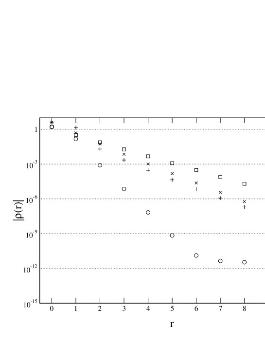
Figure 5.1: Couplings of the $\xi=2$ free scalar field in $d=2$, optimised for spatial locality ($\kappa=3$, circles: on the spatial axis, squares: on the temporal axis) and temporal locality ($\kappa=12$, pluses: on the spatial axis, crosses: on the temporal axis).

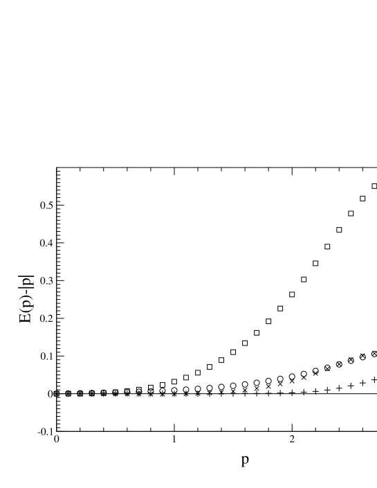
Figure 5.2: Deviations from the exact dispersion relation of the $\xi=2$ perfect action for the $d=2$ free scalar field. Circles: $\kappa=3$, $5\times 5$ couplings, squares: $\kappa=3$, $5\times$ nnt couplings, pluses: $\kappa=12$, $5\times 5$ couplings, crosses: $\kappa=12$, $5\times$ nnt couplings.

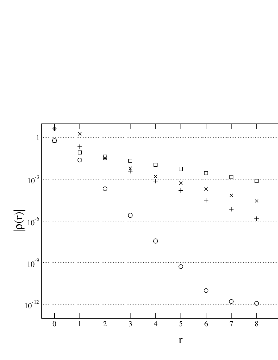
Figure 5.3: Couplings of the $\xi=4$ free scalar field in $d=2$, optimised for spatial locality ($\kappa=1.5$, circles: on the spatial axis, squares: on the temporal axis) and temporal locality ($\kappa=24$, pluses: on the spatial axis, crosses: on the temporal axis).

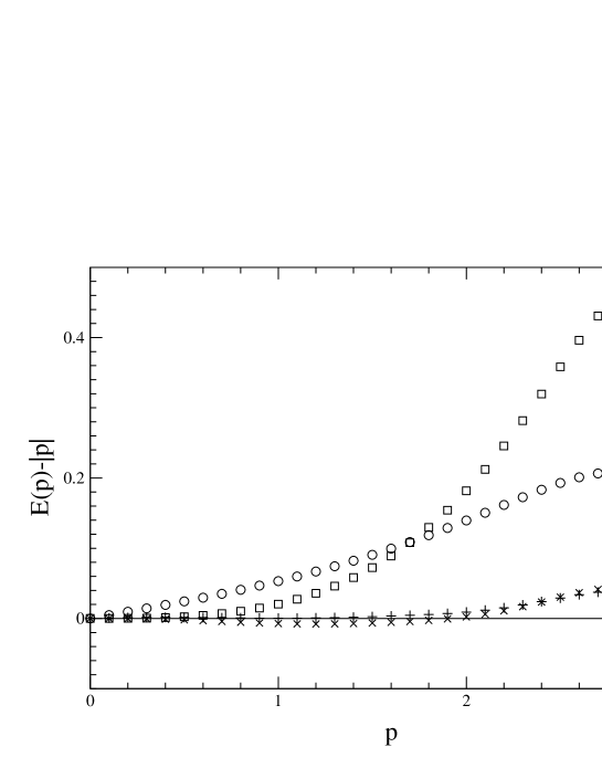
Figure 5.4: Deviations from the exact dispersion relation of the $\xi=4$ perfect action for the $d=2$ free scalar field. Circles: $\kappa=1.5$, $5\times 5$ couplings, squares: $\kappa=1.5$, $5\times$ nnt couplings, pluses: $\kappa=24$, $5\times 5$ couplings, crosses: $\kappa=24$, $5\times$ nnt couplings.

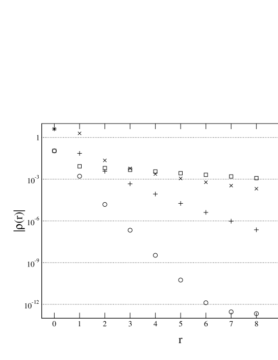
Figure 5.5: Couplings of the $\xi=10$ free scalar field in $d=2$, optimised for spatial locality ($\kappa=0.6$, circles: on the spatial axis, squares: on the temporal axis) and temporal locality ($\kappa=60$, pluses: on the spatial axis, crosses: on the temporal axis).

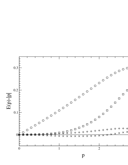
Figure 5.6: Deviations from the exact dispersion relation of the $\xi=10$ perfect action for the $d=2$ free scalar field. Circles: $\kappa=0.6$, $5\times 5$ couplings, squares: $\kappa=0.6$, $5\times$ nnt couplings, pluses: $\kappa=60$, $5\times 5$ couplings, crosses: $\kappa=60$, $5\times$ nnt couplings.

5.1.2 Spatial Blocking

For the ($d=2$) scalar field, we may perform purely spatial blockings (cf. Section 4.2) analytically and check whether (in this model) we end up with the perfect anisotropic action, eq. 5.1. We start from the isotropic FP propagator which we know analytically for a blocking that averages the continuum field isotropically around lattice sites (without overlapping):

$$D^{\text{FP}}(q) = \sum_{l=-\infty}^{\infty}\frac{1}{(q+2\pi l)^{2}}\prod_{\mu=1}^{2}\frac{\sin^{2}(q_{\mu}/2)}{(q_{\mu}/2+\pi l_{\mu})^{2}}+\frac{1}{3\kappa},$$ (5.13)

and perform a single spatial ($\mu=1$) RG step, increasing the spatial lattice spacing by a factor of two:

$$D_{\text{sp}}^{\text{FP}}(q) = \frac{1}{2}\sum_{l_{1}^{\prime}=0}^{1}\cos^{2}(\frac{q_{1}}{4}+\pi\frac{l_{1}^{\prime}}{2})D^{\text{FP}}(\frac{q_{1}}{2}+\pi l_{1}^{\prime},q_{2})+\frac{1}{6\kappa}$$ (5.14)

(note the normalisation of the $\kappa$ factor). Inserting expression eq. 5.13 and performing the substitution $q_{1}/2+\pi l_{1}^{\prime}+2\pi l_{1}\rightarrow q_{1}/2+\pi l_{1}$ we get

$$D_{\text{sp}}^{\text{FP}}(q_{1},q_{2}) = \frac{1}{2}\sum_{l=-\infty}^{\infty}\frac{1}{(\frac{q_{1}}{2}+\pi l_{1})^{2}+(q_{2}+2\pi l_{2})^{2}}\frac{\sin^{2}(\frac{q_{1}}{2})\sin^{2}(\frac{q_{2}}{2})}{(\frac{q_{1}}{2}+\pi l_{1})^{2}(\frac{q_{2}}{2}+\pi l_{2})^{2}}$$ (5.15)

$$+\frac{1}{3\kappa},$$

which is the anisotropic $\xi=2$ perfect propagator for this model, compare eq. 5.3. (Performing another single temporal RG step on this propagator gives back the initial FP propagator $D^{\text{FP}}$, which proves that the normalisation of both terms has been chosen correctly.) Of course this discussion of a single spatial RG step in the $d=2$ scalar theory cannot be generalised straightforwardly to gauge theory as the RG step cannot be treated analytically there, however these results indicate that this approach may be feasible as well for gauge theory.

5.2 Gauge Fields in the Quadratic Approximation

We will now turn to $\text{SU}(3)$ gauge fields in $d=4$ dimensions. On small fluctuations we may approximate the FP gauge action quadratically:

$$S^{\text{FP}}=\frac{1}{2N_{c}}\sum_{n,r}\rho_{\mu\nu}(r)\text{Tr}[A_{\mu}(n+r)A_{\nu}(n)]+\text{O}(A^{3})$$ (5.16)

neglecting terms of order 3 and higher in the gauge potential. In momentum space the action reads

$$S^{\text{FP}}=\frac{1}{2N_{c}}\frac{1}{V}\sum_{k}\tilde{\rho}_{\mu\nu}(k)\text{Tr}[\tilde{A}_{\mu}(-k)\tilde{A}_{\nu}(k)]+\text{O}(\tilde{A}^{3}).$$ (5.17)

The calculation of the couplings $\rho_{\mu\nu}(r)$ and the propagator $D_{\mu\nu}(r)$ is described in Appendix B.

5.2.1 Physical Quantities

Having at hand the quadratic couplings $\rho_{\mu\nu}$ and the propagator $D_{\mu\nu}$ we may easily calculate physical quantities, as e.g. the spectrum of the action or the tree level potential as described in the next sections

The Spectrum

The quadratic FP action, eq. 5.16, is defined on the lattice. Nevertheless it describes transverse massless gluons with the exact relativistic spectrum $E(k)=|\vec{k}|$ for $k_{i}=-\infty..\infty$. This is a fundamental difference to perturbatively (e.g. Symanzik) improved actions where the spectrum shows $O(a^{2})$ or $O(a^{4})$ lattice artifacts.

The spectrum is determined by looking at the singularities of the propagator $D_{\mu\nu}(k)$: We fix the momentum $\vec{k}$ and determine the corresponding energy $k_{4}$. This may be done analytically using exactly the same arguments as for the isotropic FP action (see [59]) with the result that the energy behaves as $k_{4}=-i|\vec{k}|$, where $k=q+2\pi l$, which is the exact continuum relation realised by a tower of poles in $D_{\mu\nu}$ for any given $\vec{q}$, $q_{i}\in(0,2\pi)$.

The Perturbative Potential

Another physical quantity that can be determined using the quadratic couplings is the static quark–anti-quark potential up to tree level.

At the quadratic level the potential in a finite continuum box of size $L_{s}^{3}$ is proportional to the Coulomb potential:

$$V_{\text{cont}}(\vec{x})=\frac{1}{L_{s}^{3}}\sum_{\vec{k}\neq 0}e^{i\vec{k}\vec{x}}\frac{1}{(\vec{k})^{2}},\quad where\quad k_{i}=\frac{2\pi}{L_{s}}l_{i}.$$ (5.18)

On the lattice, the corresponding relation reads

$$V_{\text{lat}}(\vec{r})=\frac{1}{N_{s}^{3}}\sum_{\vec{k}\neq 0}e^{i\vec{k}\vec{r}}D_{44}(\vec{k},k_{4}=0),$$ (5.19)

where $D_{\mu\nu}(k)$ is the propagator corresponding to the quadratic part of the lattice action. As this quantity is unchanged from the isotropic case (except a global factor $1/\xi$) the result is exactly the same as in [60]. Figure 5.7 summarises the results for the anisotropic actions. As $V\sim 1/\xi$ the deviations are accordingly smaller for larger values of the anisotropy $\xi$. Figure 5.8 compares the deviation to the continuum result of the perfect action to the deviation present with the Wilson action (for the isotropic action; the picture is exactly the same for $\xi\neq 1$) — note the difference in the scale of the deviations. It is self–evident that the perfect action heavily suppresses discretisation errors. The deviations that are still present are on one hand due to the RGT transformation not averaging exactly spherical, on the other hand due to remaining quantum fluctuations on the fine lattice.

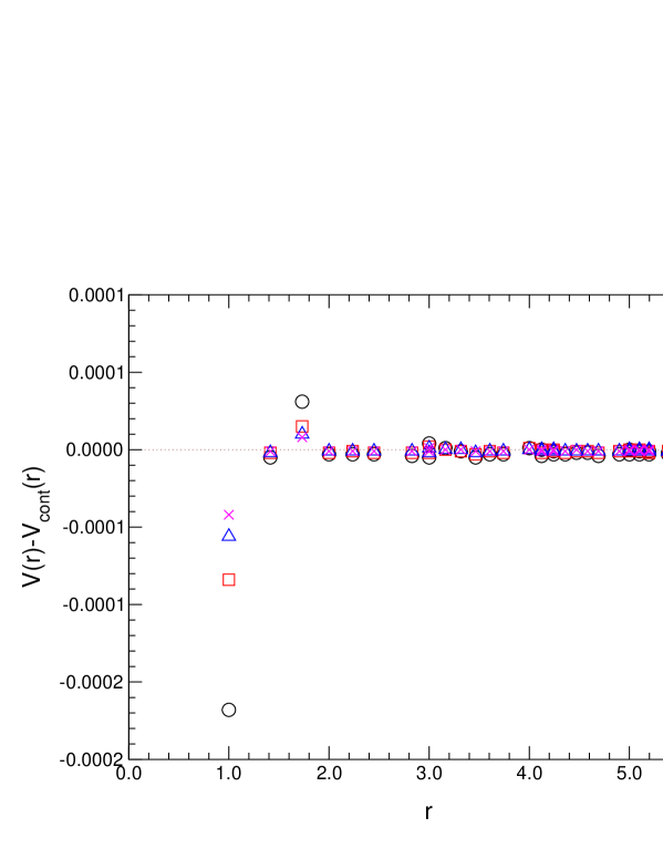
Figure 5.7: The deviations to the exact tree–level quark–anti-quark potential of the quadratic approximation to the perfect anisotropic action for $\xi=1$ (circles), $\xi=2$ (squares), $\xi=3$ (triangles), $\xi=4$ (crosses).

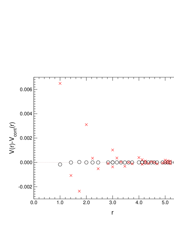
Figure 5.8: The deviations to the exact tree–level quark–anti-quark potential of the Wilson action (crosses) and the FP action (circles).

Chapter 6 The $\mathbf{\xi=}2$ Perfect Action

The main topic of this work is the construction and the application of a classically perfect gauge action for $\xi=2$ anisotropic lattices. These tasks and their results are presented in this Chapter. The construction follows the proceeding presented in Section 1.4 using the spatial blocking method and the parametrisation described in Chapter 4.

The anisotropy of the resulting action is measured using the torelon dispersion relation (see Section 2.1), the (spatial) scale is determined by the static quark-antiquark potential (see Section 2.3), where for some values of the coupling $\beta$, off-axis separations of the quarks are considered as well, to be able to estimate violations of rotational symmetry by the parametrised action. Another way of determining the (temporal) scale is the study of the deconfining phase transition (see Section 2.2), measuring the critical couplings $\beta_{\text{crit}}$ for different spatial extensions $N_{t}$ of the lattice.

Finally, the glueball spectrum is measured performing simulations at three values of $\beta$ using the $\xi=2$ action.

On one hand, the study of the classically perfect action with rather small anisotropy $\xi=2$ is a feasibility test of the ansatz as it employs only one single spatial blocking step and one single parametrisation of the resulting action. On the other hand, to determine accurately the continuum limit, one should perform simulations on fine lattices as well — using actions with large anisotropies, this may be more expensive than necessary, at least when the states to be studied are not extraordinarily heavy. The feasibility of additional spatial blocking steps, followed by parametrisations is briefly (and incompletely) checked in Chapter 7.

6.1 Construction

We construct the $\xi=2$ classically perfect anisotropic action starting with the parametrised isotropic action[2] performing one spatial blocking step as described in Chapter 4. The quadratic approximation suggests $\kappa_{t}=\xi^{2}\kappa_{s}=4\kappa_{s}$ for keeping the block transformation as close to the isotropic case as possible. Furthermore, spatial locality should stay at its optimum for the “isotropic” value of $\kappa_{s}=8.8$, thus we choose $\kappa_{t}=35.2$. Indeed, it turns out that varying $\kappa_{t}$ away from $\kappa_{t}=35.2$, keeping $\kappa_{s}=8.8$ fixed, makes it much more difficult to parametrise the resulting perfect action such that the renormalised anisotropy $\xi_{\text{R}}$ (see Section 6.2) stays close to the input value $\xi=2$.

Examining this blocking, we observe that coarse configurations obtained in a MC run with the ad-hoc anisotropic action (see Appendix D.3) are mapped to fine configurations that are close to isotropic (concerning spatial and temporal plaquette values and expectation values of the Landau gauge-fixed link variables) for input anisotropy $\xi_{\text{ad-hoc}}\approx$ 3.2.

We thus generate 20 configurations each at $\beta_{\text{ad-hoc}}=$ 2.5, 3.0, 3.5, 4.0 using the ad-hoc anisotropic action with $\xi_{\text{ad-hoc}}$=3.2. These configurations are spatially blocked using the isotropic action $\mathcal{A}_{5}^{444}$ (see Appendix D.2) to describe the isotropic minimised configuration on the r.h.s. of eq. 1.5.

To construct the action we follow the procedure described in Sections 1.4.3–1.4.5. Several non-linear fits are performed for the derivatives of 20 configurations at $\beta=3.5$, using different sets of parameters. Concerning the non-linear parameters, we find out that it is necessary to keep all asymmetry parameters $\eta_{i}$ non-zero. Moreover, it is crucial to distinguish the $c_{i}$ parameters for different plaquette orientations, see Table 4.1 and Section 4.3.4. The parameters $c_{i}$ are chosen to be non-zero for $i=1,2,3$ as adding additional free $c_{4}$ parameters does not improve $\chi^{2}$ significantly.

Having fixed the non-linear parameters $\eta$ and $c_{i}$, we include the derivatives of 20 configurations at $\beta=4.0$ and the action values of all the configurations at $\beta=$ 3.5, 4.0 in the linear fit, keeping the non-linear parameters fixed. The resulting values of $\chi^{2}$ and the linear behaviour of the actions suggest a linear set with $\max(k+l)_{\text{sp}}=4$, $\max(k+l)_{\text{tm}}=3$ where the action values are included with weights $w_{\text{act}}=0.018$ relative to the derivatives (see also Figure 1.3). Using this value, the good parametrisation of the derivatives obtained in the full nonlinear fit is preserved, at the same time the mean error of the action value due to the parametrisation is as small as 0.35%.

It is checked that the values of $\chi^{2}$ are still acceptable on sets of configurations down to $\beta=3.0$, besides that they do not increase significantly for configurations independent of the ones used in the fitting procedure. The behaviour of the linear parameters of the action as a function of the simple plaquette values $u$ and smeared plaquette values $w$ is displayed in Figure 6.1, the parameters of the resulting action are listed in Appendix D.4.

\psfrag{action}{$\mathcal{A}(u,w)$}\psfrag{u}{$u$}\psfrag{w}{$w$}\includegraphics[width=227.62204pt]{uw_xi2_ss.eps}

\psfrag{action}{$\mathcal{A}(u,w)$}\psfrag{u}{$u$}\psfrag{w}{$w$}\includegraphics[width=227.62204pt]{uw_xi2_st.eps}

Figure 6.1: The behaviour of the linear parameters $p_{kl}$ as a function of the values of the standard plaquette ($u$) and the smeared plaquette ($w$) for the parametrisation of the classically perfect $\xi=2$ action.

6.2 The Renormalised Anisotropy

The renormalised anisotropy $\xi_{R}$ of the action presented above is measured using the torelon dispersion relation as described in Section 2.1. The main advantage of this approach is obtaining the renormalised anisotropy $\xi_{R}$ as well as an estimate for the scale $a_{s}$, $a_{t}$ performing computationally rather inexpensive measurements.

6.2.1 Details of the Simulations and Results

The parameters of the simulations carried out are collected in Table 6.1.

$\beta$	$S^{2}\times L\times T$	# sweeps / measurements
3.00	$8^{2}\times 4\times 20$	72000 / 14400
3.15a	$8^{2}\times 5\times 20$	54000 / 10800
3.15b	$5^{2}\times 8\times 20$	47600 / 9520
3.30	$12^{2}\times 6\times 30$	35600 / 7120
3.50a	$12^{2}\times 8\times 24$	39400 / 7880
3.50b	$14^{2}\times 6\times 30$	36800 / 7360

Table 6.1: Run parameters for the torelon measurements using the $\xi=2$ perfect action. The lattice extensions in torelon direction $L$, the extension in the two transversal spatial directions $S$ as well as the temporal extension $L$ are given.

The Polyakov line around the short spatial direction is measured on APE-smeared configurations of smearing levels 3, 6, 9, 12, 15 for $\beta\geq 3.3$ and 2, 4, 6, 8, 10 for $\beta\leq 3.15$ with smearing parameter $\lambda_{s}=0.1$ (see Section 2.1.2). The measured energies $E(p^{2})$ determined using variational methods (see Appendix E) depending on the lattice momentum $p^{2}$ are given, together with the number of operators used in the variational method, the fit ranges and the values of $\chi^{2}$ per degree of freedom, $\chi^{2}/N_{\text{DF}}$, in Tables G.1, G.2 in Appendix G. The two simulations denoted by $3.15^{b}$ and $3.50^{b}$ are used to check the stability of the method. The first one is carried out on a lattice with small transversal spatial size (the torelon string measured is even longer), the latter is measuring the energies of a rather short string.

Figures 6.2–6.7 display the dispersion relations at the different values of the coupling $\beta$ including all values of $p$ at which the energies could be determined on the lattices considered. Note, that the energies of the $p=0$ torelons (the torelon masses) may be hard to determine because the effective masses do not reach a plateau within the temporal extent of the lattice; however, using the non-zero momentum energies, the masses may still be accurately determined.

To determine the renormalised anisotropy $\xi_{R}$ as well as the torelon mass in units of the temporal lattice spacing $ma_{t}$ we employ fully correlated fits over different ranges of $p^{2}$ and choose the values depending on $\chi^{2}/N_{\text{DF}}$ and the precision of the dispersion relation data in the respective range. The results are given in Table 6.2.

$\beta$	fit range	$\xi_{R}$	$m_{\text{T}}a_{t}$	$\chi^{2}/N_{\text{DF}}$
3.00	0..5	1.903(81)	1.324(98)	0.39
3.15a	0..4	1.966(39)	0.700(35)	0.83
3.15b	0..5	2.022(104)	1.262(84)	0.62
3.30	1..9	1.912(9)	0.311(5)	0.94
3.50a	1..10	1.836(9)	0.149(10)	0.94
3.50b	1..8	1.826(16)	0.208(16)	1.61

Table 6.2: Results of the torelon simulations using the $\xi=2$ perfect action. The fit range in $p^{2}$ is given in units of $(2\pi/S)^{2}$.

Using the finite size relation for the torelon mass corresponding to eq. 2.1:

$$M_{T}(La_{s})=(\sigma+\frac{D}{(La_{s})^{2}})La_{s}$$ (6.1)

it is possible to calculate the string tension $\sigma$ and thus the spatial scale $a_{s}$. The string model predicts $D=-\frac{\pi}{3}$ for long strings. To estimate the scale using the results of the torelon simulation, we use this string picture value and stay aware that the estimate gets worse for short strings. To obtain the hadronic scale $r_{0}$ and the lattice spacings we employ $r_{0}\sqrt{\sigma}$=1.193(10) from [2] and use the definition $r_{0}=0.50$ fm. The results are collected in Table 6.3.

The scale is measured accurately using the static quark-antiquark potential (see Section 6.3) such that we can compare our torelon estimates to the true value. This is done in Table 6.4 and it turns out that the deviation of the torelon estimates for the scale $r_{0}/a_{s}$ to the much more reliable potential values does not exceed about 6% if the length of the string is not too short (say $La_{s}\gtrsim 1$ fm). For short strings, the string picture does not apply, we may therefore not expect good results in this case. But even for very long strings, it is not possible to obtain very accurate information about the (hadronic) scale. Firstly, long strings are very heavy and thus difficult to measure (comparable to the very long range region of the static quark-antiquark potential), especially when the anisotropy $\xi$ is not very large; and secondly, using the string tension $\sigma$ to set the scale is plagued by ambiguities. Depending on the analysis of the respective potential measurements, $r_{0}\sqrt{\sigma}$ may vary as much as about 4% (see Section 3.4.3) and additionally, the effective string tension at separations around $r=1$ fm does not correspond to $\sigma$ occurring with the torelon strings.

There seems to be no problem if the transverse volume is rather small as in the $\beta=3.15^{b}$ simulation, except of course the large momenta occurring which make the determination of the energies more difficult. As well, the estimates of the renormalised anisotropy $\xi_{R}$ do not show significant deviations neither for small transverse volume nor for short strings.

$\beta$	$\sqrt{\sigma}a_{s}$	$r_{0}/a_{s}$	$a_{s}$ [fm]	$a_{t}$ [fm]
3.00	0.834(20)	1.43(5)	0.350(12)	0.184(14)
3.15a	0.563(8)	2.12(5)	0.236(6)	0.120(5)
3.15b	0.579(18)	2.06(8)	0.243(9)	0.120(11)
3.30	0.3578(21)	3.33(5)	0.150(2)	0.079(1)
3.50a	0.225(5)	5.31(16)	0.094(3)	0.051(2)
3.50b	0.304(7)	3.92(12)	0.128(4)	0.070(3)

Table 6.3: Estimates of the scale determined from torelon results (see Table 6.2), see text.

$\beta$	$La_{s}$ [fm]	$r_{0}/a_{s}$ (Torelon)	$r_{0}/a_{s}$ (Potential)	rel. error
3.00	1.48	1.43(5)	1.353(16)	+5.7%
3.15a	1.23	2.12(5)	2.038(2)	+4.0%
3.15b	1.96	2.06(8)	2.038(2)	+1.1%
3.30	0.95	3.33(5)	3.154(8)	+5.6%
3.50a	0.82	5.31(16)	4.906(21)	+8.2%
3.50b	0.61	3.92(12)	4.906(21)	-20.0%

Table 6.4: The estimates of the scale obtained from torelon measurements (see. Table 6.3) compared to the scale measured using the static quark-antiquark potential (see Table 6.6). The length of the torelon string $La_{s}$ in physical units is given as well.

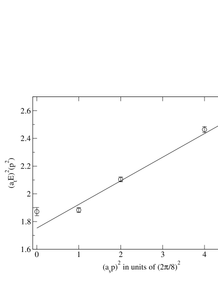
Figure 6.2: Torelon dispersion relation for $\beta=3.0$. The straight line is the correlated fit to $E^{2}(p)=m_{T}^{2}+p^{2}$ in the range $p^{2}=0..5$.

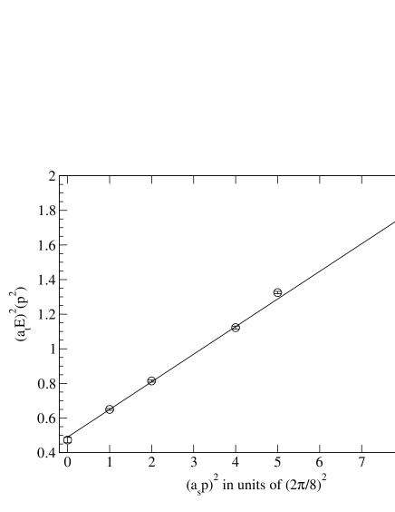
Figure 6.3: Torelon dispersion relation for $\beta=3.15^{a}$. The straight line is the correlated fit to $E^{2}(p)=m_{T}^{2}+p^{2}$ in the range $p^{2}=0..4$.

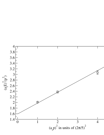
Figure 6.4: Torelon dispersion relation for $\beta=3.15^{b}$ on a small transverse volume. The straight line is the correlated fit to $E^{2}(p)=m_{T}^{2}+p^{2}$ in the range $p^{2}=0..5$.

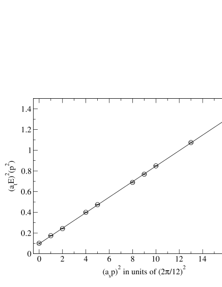
Figure 6.5: Torelon dispersion relation for $\beta=3.3$. The straight line is the correlated fit to $E^{2}(p)=m_{T}^{2}+p^{2}$ in the range $p^{2}=1..9$.

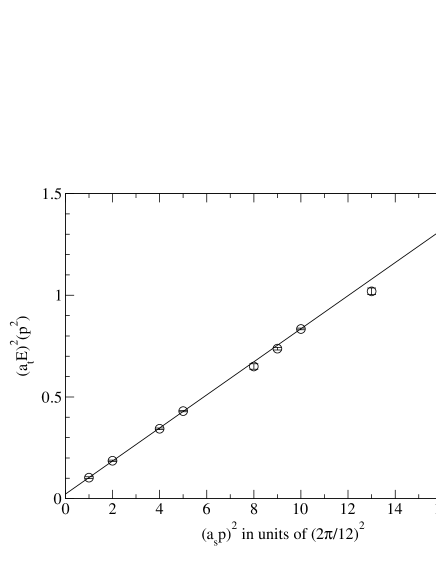
Figure 6.6: Torelon dispersion relation for $\beta=3.5^{a}$. The straight line is the correlated fit to $E^{2}(p)=m_{T}^{2}+p^{2}$ in the range $p^{2}=1..10$.

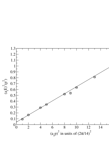
Figure 6.7: Torelon dispersion relation for $\beta=3.5^{b}$ for a short torelon string. The straight line is the correlated fit to $E^{2}(p)=m_{T}^{2}+p^{2}$ in the range $p^{2}=1..8$.

Finally, we may conclude that determining the renormalised anisotropy using the torelon dispersion relation is a stable and apparently sensible procedure. There are no manifest problems and it works for coarse and fine lattices as well. Checks employing different lattice extensions indicate that the determination of the renormalised anisotropy is very stable. The estimate of the lattice scale, however, is not very accurate, mainly due to the use of the string picture relation, eq. 6.1; the (systematic) error of the torelon scale is about 5% for sensible torelon lengths $L\gtrsim 1$ fm with a tendency of underestimating the lattice spacing $a_{s}$.

Choosing the lattice size, one has to pay attention on one hand to the length of the torelon string, i.e. the extension of the (short) longitudinal direction: if the string is too short, there is no useful estimate for the scale; if it is much too long, it will be difficult to measure due to its high energy. On the other hand, the transversal direction in principle may be short in order to make the simulation cheaper what concerns computational effort, however, if it is too short, the momenta are large, and again the measurement becomes difficult. Finally, the temporal extension should be chosen large enough such that the torelon mass (which may be rather light) may be determined directly.

6.3 The Scale

To set the scale of the action at a given $\beta$-value we measure the quark-antiquark potential (see Section 2.3) and determine the Sommer scale $r_{0}\approx$ 0.50 fm. For the anisotropic action, we still employ the definition of $r_{0}$:

$$r^{2}V^{\prime}(r)|_{r=r_{0}}=1.65,$$ (6.2)

however $V(r)$ is now measured in units of the temporal lattice spacing and thus:

$$-\alpha+\xi\hat{\sigma}(\frac{r_{0}}{a_{s}})^{2}=1.65,$$ (6.3)

where $\hat{\sigma}$ denotes the fitted dimensionless value $\hat{\sigma}=\sigma a_{s}a_{t}$ of the string tension. The renormalised anisotropy $\xi$ thus has to be known before the spatial scale $r_{0}$ may be determined.

The static quark-antiquark potential is measured on lattices of different scales. The measurements at $\beta=3.00$, 3.30 include the determination of the potential between quarks that are off-axis separated along the lattice vectors (1,0,0), (1,1,0), (1,1,1), (2,1,0), (2,1,1), (2,2,1) (and lattice rotations) in order to estimate violations of rotational symmetry. The rest of the measurements include only on-axis separations due to the large computational cost (concerning speed and memory) of the off-axis measurement. The parameters of the simulations are given in Table 6.5.

$\beta$	off-axis sep.	$S^{3}\times T$	# sweeps / measurements
3.00	yes	$8^{3}\times 16$	42000 / 2800
3.15	no	$10^{3}\times 20$	39800 / 3980
3.30	yes	$10^{3}\times 20$	27000 / 1800
3.50	no	$12^{3}\times 24$	36400 / 3640

Table 6.5: Run parameters for the measurements of the static quark-antiquark potential using the $\xi=2$ perfect action.

The values of the off-axis potential $a_{t}V(\vec{r})$ at $\beta=3.30$ are collected in Table G.4 in Appendix G and displayed in Figure 6.8, the values of the off-axis potential on the coarse lattice at $\beta=3.00$ are collected in Table G.3. The potential values $a_{t}V(r)$ of the on-axis simulations are collected in Table G.5.

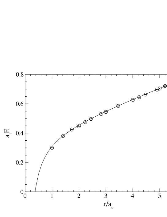
Figure 6.8: Ground state of the static quark-antiquark potential at $\beta=3.3$. Including a global fit to the Cornell potential in the range $r=\sqrt{2}..5$.

The parameters $\alpha$ and $\sigma$ (the string tension) in the Cornell potential, eq. 2.24, are determined using global fits, the hadronic scale $r_{0}$ is determined performing local fits. The fit ranges and results are given in Table 6.6. In the global fit to the off-axis potential at $\beta=3.30$ we exclude the badly measured separations $2(2,1,0)$ and $2(2,1,1)$.

$\beta$	gl. fit	$\alpha$	$\sigma a_{s}a_{t}$	loc. fit	$r_{0}/a_{s}$	$r_{0}\sqrt{\sigma}$
3.00	$1-2\sqrt{6}$	-0.201(18)	0.3595(87)	$\sqrt{6}-3$	1.353(16)	1.119(51)
3.15	$1-5$	-0.1503(12)	0.1654(6)	$1-3$	2.038(2)	1.162(15)
3.30	$\sqrt{2}-5$	-0.1539(7)	0.0683(3)	$2\sqrt{2}-2\sqrt{3}$	3.154(9)	1.140(8)
3.50	$1-6$	-0.1478(4)	0.0320(3)	$2-4$	4.906(21)	1.189(14)

Table 6.6: Results of the measurements of the static quark-antiquark potential using the $\xi=2$ perfect action. The parameters $\alpha$ and $\sigma$ of the Cornell potential are given together with the global fit range chosen to determine them. The hadronic scale $r_{0}$ is given in spatial lattice units together with the local fit range used to determine that quantity. Note, that $c=6.00$ has been chosen for $\beta=3.0$ and $c=0.89$ has been chosen for $\beta=3.5$ (see Section 2.3.4). Additionally, the dimensionless quantity $r_{0}\sqrt{\sigma}$ is given.

In principle, it is possible to determine the renormalised anisotropy using the first excited state of the potential together with the ground state. As can be seen from Figure 6.9 however, for the off-axis potential at $\beta=3.3$, the energy values of the first excited state have large errors. The result for the separation $a_{t}(V^{*}(r_{0})-V(r_{0})$=0.555(47) thus shows a large error. Comparing this value to $r_{0}(V^{*}(r_{0})-V(r_{0}))\approx 3.25(5)$ of [146] one obtains $\frac{r_{0}}{a_{t}}=5.86(59)$ and thus $\xi_{\text{R}}=a_{s}/a_{t}$=1.86(19) for $\beta=3.3$ which is in agreement with the value determined using the torelon dispersion relation, $\xi_{\text{R}}$=1.912(9). A similar determination for the on-axis potential at $\beta=3.50$ is even more difficult due to the small number of data. The result is $\xi_{\text{R}}$=1.66(32) which does again agree with the torelon result, $\xi_{\text{R}}=1.836(9)$. Due to the large errors (caused by the choice of $\beta$ and the operators used) this method of determining the renormalised anisotropy $\xi_{\text{R}}$ is not suitable in the context of this work. However, for the determination of the scale as well as of the anisotropy on lattices with finer temporal lattice spacing (above all with higher anisotropies) this way might be feasible at least if off-axis separations are included in the measurement.

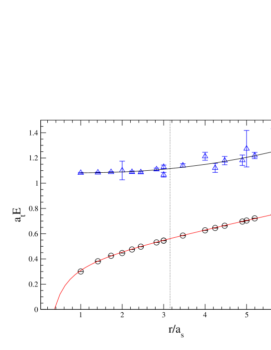
Figure 6.9: Static quark antiquark potential at $\beta=3.3$ including the first excited state $V^{*}(r)$ at $\beta=3.3$. The ground state values are again fitted to the ansatz $V(r)=V_{0}+\alpha/r+\sigma r$, whereas the values of the excited state are fitted to the (ad-hoc) ansatz $V^{*}(r)=A/r+B+Cr+Dr^{2}$. The value of $r_{0}$ where the determination of the anisotropy is done, using the gap, is marked by the dotted line.

The measurements at $\beta=3.0,3.3$ including a large number of off-axis separations provide information about the deviations from rotational invariance. This issue has been addressed in [60] for the renormalisation group used in this work. It turned out that violations of rotational symmetry caused by the blocking are small (see also Section 5.2.1). That this is still true for the parametrisation employed is shown by the off-axis potential, see Figure 6.8. The deviations on the coarse lattice at $\beta=3.00$ are significantly larger (see Figure 6.10) which is no surprise as this coupling corresponds to a spatial lattice spacing $a_{s}\approx 0.37$ fm.

The static $q\bar{q}$ potential is an effective test of scaling. Expressing the potential measurements performed at different couplings $\beta$ in the RG invariant, dimensionless ratios $r/r_{0}$ and $r_{0}V$, subtracting the unphysical constant $r_{0}V(r_{0})$ should lead to potentials lying exactly on top of each other. Deviations indicate either scaling violations or ambiguities in the determination of $r_{0}$. Figure 6.10 which includes all potential measurements shows that the different curves can hardly be distinguished from each other, except some energies determined on the coarse lattice at $\beta=3.00$ that deviate notably from the curve which is a fit to the Cornell potential including all the measurements that have been included into the global fits of the single $\beta$ values, see Table 6.6. The results for the two physical parameters are $\alpha=-0.27799(5)$ and $\sigma r_{0}^{2}$=1.3690(3).

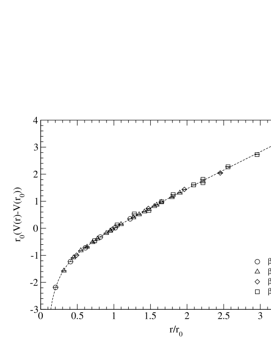
Figure 6.10: The static quark-antiquark potential measurements expressed in RG invariant, dimensionless units $r/r_{0}$, $r_{0}V$. The unphysical constant $r_{0}V(r_{0})$ has been subtracted such that all the curves exactly coincide at $r=r_{0}$. The dashed line is a global fit to the Cornell potential, eq. 2.24.

6.4 The Critical Temperature

Another interesting quantity to study with the $\xi=2$ perfect action is the critical temperature of the deconfining phase transition, see Section 2.2. This quantity contains mainly information about the temporal scale of the lattice at a given coupling $\beta$ as $T_{c}=1/(N_{t}a_{t})$. Comparing this information to quantities obtained from the measurements of torelons or the static quark-antiquark potential offers a lot of possibilities of scaling (and other) tests. Because measurements of these quantities at the determined values of $\beta_{\text{crit}}$ are yet absent and because interpolations in $\beta$ are very difficult, because of the renormalisation of the anisotropy $\xi$ which is another parameter entering, these tests are a future project.

In this first study, we decide not to examine the finite-size scaling of $\beta_{\text{crit}}$ but to choose $L_{s}/L_{t}=\xi\cdot N_{s}/N_{t}\approx 3.5\sim 4$. Obviously, the anisotropic nature of the action makes the computational effort of the simulations for exploring the deconfining phase transition smaller. The effects of the finite volume are (rather conservatively) estimated by using the finite-size scaling relation for $\beta_{\text{crit}}$, eq. 3.2. The parameter $|h|$ is set to the largest value $|h|=0.25$ that has been observed with the isotropic action, the value of $\xi_{\text{R}}$, used to estimate the spatial lattice volume, is set to the lowest value appearing in the whole range of $\beta$ values considered. These finite-volume errors are given together with the run-time parameters and results of the $\xi=2$ simulations in Table 6.7. Figures 6.11–6.15 show that the determination of $\beta_{c}$ is rather precise, partly due to the reweighting technique. As well, it shall be understood that in order to make the results even more precise, a finite-size extrapolation is indispensable.

lattice size	$\beta$	sweeps	$\tau_{p}$	$\tau_{\text{int}}$	$\chi_{\text{L}}$	$\beta_{c}$
$3\times 6^{3}$	2.80	45000		70	1.45(5)	2.863(1)(5)
	2.85	45000	410	259	11.3(20)
	2.87	45000		312	21.6(28)
	2.90	50000		100	2.34(10)
$4\times 8^{3}$	3.00	45000		81	1.63(5)	3.032(1)(5)
	3.02	45000	870	102	3.97(26)
	3.03	45000	830	372	43.2(22)
	3.04	45000		188	10.9(18)
	3.05	55600		144	3.94(21)
$5\times 9^{3}$	3.07	44000		117	0.84(4)	3.118(1)(6)
	3.10	45000	560	154	4.38(63)
	3.11	20500	640	198	15.0(27)
	3.12	44500	3700	278	33.2(19)
	3.15	20000		110	3.26(18)
$6\times 11^{3}$	3.17	45000	1440	121	7.4(11)	3.181(1)(6)
	3.18	45000	1750	201	30.0(15)
	3.185	45000		232	23.2(24)
	3.19	45000		123	10.4(14)
	3.20	45000		100	5.62(36)
$7\times 13^{3}$	3.22	32400	700	87	6.7(5)	3.236(1)(6)
	3.23	44500	750	129	18.4(11)
	3.24	29000		149	20.7(16)
	3.25	22400		83	9.2(10)

Table 6.7: Run-time parameters of $\xi=2$ $T_{c}$-simulations. The number of sweeps, the persistence time $\tau_{p}$ (if definable), the integrated autocorrelation time $\tau_{\text{int}}$ and the Polyakov loop susceptibility $\chi_{\text{L}}$ are given for all values of $\beta$ used in the final reweighting procedure, as well as the resulting $\beta_{c}$. The systematic error in the second brackets is a (rather conservative) estimate of the finite volume effects and has to be considered if the given value should be an estimate of the infinite-volume critical coupling.

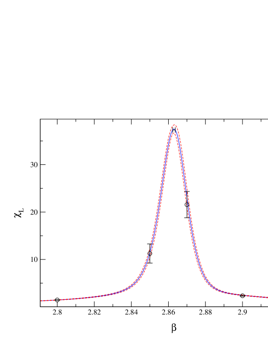
Figure 6.11: The Polyakov loop susceptibility on the $3\times 6^{3}$ lattice for the $\xi=2$ perfect action. The solid curves are the interpolations using Ferrenberg-Swendsen reweighting, the dashed lines indicate the bootstrap error.

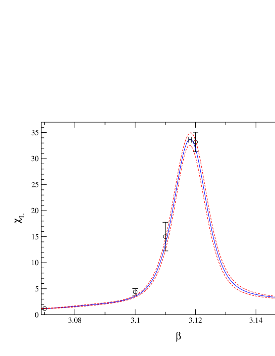
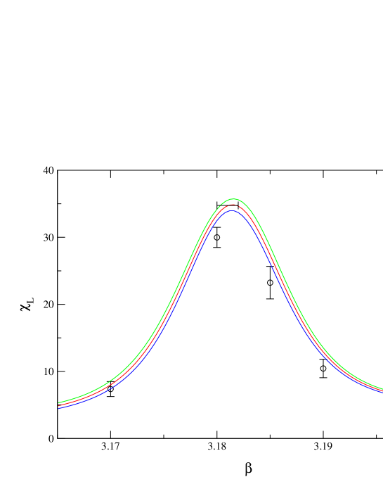
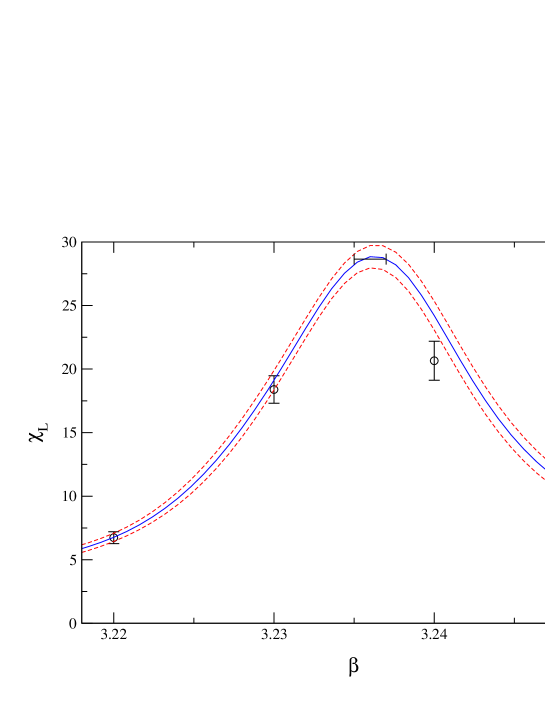
Figure 6.12: The Polyakov loop susceptibility on the $4\times 8^{3}$ lattice for the $\xi=2$ perfect action. The solid curves are the interpolations using Ferrenberg-Swendsen reweighting, the dashed lines indicate the bootstrap error.

Figure 6.13: The Polyakov loop susceptibility on the $5\times 9^{3}$ lattice for the $\xi=2$ perfect action. The solid curves are the interpolations using Ferrenberg-Swendsen reweighting, the dashed lines indicate the bootstrap error.

Figure 6.14: The Polyakov loop susceptibility on the $6\times 11^{3}$ lattice for the $\xi=2$ perfect action. The solid curves are the interpolations using Ferrenberg-Swendsen reweighting, the dashed lines indicate the bootstrap error.

Figure 6.15: The Polyakov loop susceptibility on the $7\times 13^{3}$ lattice for the $\xi=2$ perfect action. The solid curves are the interpolations using Ferrenberg-Swendsen reweighting, the dashed lines indicate the bootstrap error.

6.5 Glueballs

Finally, our $\xi=2$ classically perfect action is used to determine the glueball spectrum in pure lattice gauge theory (cf. Section 2.4). As glueballs are rather heavy, $m_{G}\gtrsim 1.5$ GeV, to study their masses the use of anisotropic lattices is particularly useful.

Due to mixing with other states existing in pure gauge theory on a periodic lattice, such as torelons or glueball pairs, and due to the breaking of the continuum rotational symmetry by the lattice which leads to glueball states transforming under the cubic group (see Section 2.4), the identification and the continuum spin assignment of single glueball states are additional vital questions which will be addressed in Sections 6.5.3, 6.5.5. Finally, the resulting energies of all the states that can be measured and assigned a value of continuum spin to, are given in units of the hadronic scale $r_{0}$ as well as in MeV for convenience.

6.5.1 Simulation Parameters

To allow a continuum extrapolation, at least for the lighter states, we decide to perform simulations at three different lattice spacings in the range 0.10 fm $\leq a_{s}\leq$ 0.25 fm in volumes between (1.2 fm)³ and (2.0 fm)³. The simulation parameters are given in Table 6.8. The gauge fields are updated by performing compound sweeps consisting of 4 pseudo over-relaxation and 1 Metropolis sweep (see Sections 8.1.1, 8.1.2), and after every 2 compound sweeps we measure all 22 loop shapes up to length 8 (see Figure 2.7). The measurement is performed on APE-smeared configurations (see Section 2.1.2) to spatially enlarge the operators, thus improving the overlap with the glueball states, and to reduce unphysical high-momentum fluctuations. On the coarse lattice at $\beta=3.15$ we use smearing levels $2,4,6,8,10$, on the other lattices we use levels $3,6,9,12,15$, always with smearing parameter $\lambda_{s}=0.1$. The measured operators are projected into all the irreducible representations of the cubic group. We measure all possible polarisations to suppress statistical noise (see Section 2.4.2).

$\beta$	$(a_{s}/r_{0})^{2}$	$S^{3}\times T$	$V$	# sweeps / measurements
3.15	0.2408(5)	$8^{3}\times 16$	(1.96 fm)3	241000 / 24100
3.30	0.1005(6)	$10^{3}\times 20$	(1.59 fm)3	99000 / 9900
3.50	0.0415(4)	$12^{3}\times 24$	(1.22 fm)3	115000 / 11500

Table 6.8: Run parameters for the glueball simulations using the $\xi=2$ perfect action.

6.5.2 Determination of the Energies

The masses of the lowest states and the first excited states (if possible) in all the representations are determined using the variational methods and techniques described in Appendix E. The results in units of the temporal lattice spacing $a_{t}$ are listed in Tables G.6 – G.8 in Appendix G together with the number $N$ of operators entering into the fitting procedure, the time slices on which the initial generalised eigenvalue problem is solved (usually 1/2), the number of operators $M$ in the final fit and the corresponding value of $\chi^{2}/N_{\text{DF}}$. These results are then multiplied by $\xi_{R}\cdot r_{0}/a_{s}$ to obtain the glueball masses in units of the hadronic scale $r_{0}$, listed in Table 6.9.

In order to obtain reliable estimates of the glueball masses from the variational method, one has to pay attention that among the large number of operators (up to 145 on five smearing levels) there are no correlators entering the process that are measured exceptionally bad, i.e. with large errors even at small time separation, as this may destabilise the method. To filter out such data, we calculate the “correlator lifetimes” defined in Section 2.4.2 and drop all correlators whose lifetime is smaller than a given minimum. Usually, this is repeated with different minimal values, yielding different sized sets of operators ($2\sim 4$ sets per representation). The $O(100)$ mass determinations using different parameter sets (see Appendix E) are then carried out on each set of initial operators, and it turns out that generally the variational method used is stable, provided that the badly measured operators are absent from the beginning and provided that no important operators are missing. Patently, having such a window of the number of initial operators may be difficult if there is a rather small number of operators.

For some heavy states, such as the $PC=--$ glueballs, whose masses could only be determined from the $\beta=3.50$ measurements, we have to resort to using the correlators at $t_{0}=0$ and $t_{1}=1$ for the solution of the first generalised eigenvalue problem, eq. E.3, yielding the lowest lying dual vectors $v_{n}$, $n=1,\ldots,M$, that are used in the subsequent optimisation. This has the advantage that the correlators from separation $t_{0}=0$ are positive definite by definition (which is not true for $t_{0}\geq 1$), thus rendering the second generalised eigenvalue problem, eq. E.8, well defined even if all initial operators are kept, $M=N$. However, the correlators $C(t=0)$ are under suspicion of containing rather little physical information about the correlation lengths (which correspond to the decay of the correlators), actually they almost only provide information about the relative normalisation of operators. Obviously, operators with a large signal at $t=0$ might be preferable because their signal/noise ratio is probably rather better on average, however in general they do not correspond to the operators having the largest overlap with the lowest-lying states. It turns out that using $t_{0}=0$, $t_{1}=1$ one has to pay much more attention in choosing the fit range $t=t_{\text{min}}\ldots t_{\text{max}}$ because at small $t$ the contamination of the lowest masses due to higher states is much more significant.

During the analysis, it turns out that the mass determinations for the scalar representation $A_{1}^{++}$ are rather challenging. The ground state receives a larger relative error than comparable states where the operators are measured about as well; for the first excited state it is very hard to obtain a stable determination, and the error of its mass may turn out to be huge (e.g. at $\beta=3.50$). Probably, it is the underlying vacuum, having the same quantum numbers as the glueball state, that is responsible for these troubles. As already specified in Section 2.4.2 we treat the vacuum just like another state in this representation, such that the glueball ground state is effectively a first excited state and the glueball first excited state is effectively a second excited state of the representation. Attempts of using other ways of getting rid of the vacuum such as the usual subtraction or the subtraction of large $t$ correlators (that are assumed to contain solely noise, however correlated to the noise at lower $t$) or even more sophisticated methods (like solving a generalised eigenvalue problem using large $t$ correlators to dig out the vacuum state) do not at all succeed in improving the situation.

Channel	$J$	$\beta=3.15$	$\beta=3.30$	$\beta=3.50$
$A_{1}^{++}$	0	2.58(9)	3.55(13)	3.65(15)
${A_{1}^{++}}^{*}$	0	5.47(53)	6.83(37)	6.49(148)
$E^{++}$	2	5.63(23)	5.93(15)	6.08(28)
${E^{++}}^{*}$	2	7.95(73)	8.76(48)	10.66(59)
$T_{2}^{++}$	2	5.67(25)	5.82(13)	6.13(16)
${T_{2}^{++}}^{*}$	2		7.97(69)	10.16(30)
$A_{2}^{++}$	3	6.71(73)	9.11(64)	10.92(48)
${A_{2}^{++}}^{*}$				14.12(130)
$T_{1}^{++}$	3	7.54(68)	9.00(44)	11.21(33)
${T_{1}^{++}}^{*}$		8.69(91)
$A_{1}^{-+}$	0	6.36(59)	6.13(28)	6.79(27)
${A_{1}^{-+}}^{*}$				10.27(110)
$E^{-+}$	2	7.41(48)	8.23(28)	8.48(29)
${E^{-+}}^{*}$		8.35(125)		12.66(84)
$T_{2}^{-+}$	2	7.41(49)	8.18(21)	8.57(42)
${T_{2}^{-+}}^{*}$				15.08(67)
$T_{1}^{+-}$	1	7.20(39)	7.69(26)	9.12(24)
$A_{2}^{+-}$	3			11.02(68)
${A_{2}^{+-}}^{*}$				15.55(147)
$T_{2}^{+-}$		7.75(87)		10.29(118)
${T_{2}^{+-}}^{*}$				14.98(139)
$E^{+-}$				12.42(42)
$T_{1}^{--}$				10.81(83)
$T_{2}^{--}$				10.85(83)
$A_{2}^{--}$				12.18(45)
$A_{1}^{--}$				15.34(103)

Table 6.9: Final glueball mass estimates in terms of the hadronic scale $r_{0}$, $m_{G}r_{0}$ from the measurements using the perfect $\xi=2$ action. The continuum spin assignment $J$ is given as well.

6.5.3 Identification of Glueballs

Besides single glueballs, the spectrum of pure gauge theory on a lattice with periodic boundary conditions also contains states consisting of several glueballs, torelons or mixed states of glueballs and torelons. Although we expect that the operators used to measure glueball energies couple most strongly to the single glueball states, other states with similar masses and compatible quantum numbers might mix with them and distort the result, i.e. the energy determined by the analysis of the correlation matrix may be dominated by a multi-glueball or torelon state with smaller energy than the single-glueball state to be measured.

In principle, there are several means of determining the nature of a state that has been measured. Firstly, the simulation may be repeated on lattices of different size, keeping the lattice spacing fixed. As multi-glueball and torelon states show a finite-volume behaviour very different from single glueballs, such states stand out and may be dropped from further analysis. Secondly, one may measure additional operators that couple strongly to torelon or multi-glueball states. Including and excluding these operators in the variational method and studying the coefficients obtained from the optimisation, the mixing strength is determined and states which do not mix considerably with any of the additional operators may be safely considered to be single-glueball states. Finally, using the mass estimates for the low-lying glueballs, one may determine the approximate locations of the lowest-lying multi-glueball states. Also, the minimal energy of mixing torelons may be estimated using the string formula, eq. 2.1.

Torelons

The first two of the methods mentioned above require additional work and computer time and go beyond the scope of this work. The last method, however, can be done rather easily. Let us first calculate the energy of the lowest-lying torelon states that may interfere with our measurements. Single torelons (see Section 2.1) transform non-trivially under $Z_{3}$ symmetry operations; our operators, closed Wilson loops, however, are invariant under these transformations. This means that they cannot create single torelon states, however the creation of two torelons of opposite center charge is possible. We assume that they do not interact considerably and that our lattice extension is rather large and thus we use the simple formula $E_{2T}\approx 2\sigma L$ to estimate the energy of a torelon pair with momentum zero, where $\sigma$ is the string tension (measured by the static $q\bar{q}$ potential, see Section 6.3) and $L$ is the spatial extent of the lattice. Table 6.10 lists the minimum energies of torelon pairs to be expected on our lattices.

$\beta$	$r_{0}E_{2T}$
3.15	10.60
3.30	8.24
3.50	6.92

Table 6.10: The minimum energies of momentum zero torelon pairs on the lattices used in the glueball simulations, given in units of $r_{0}^{-1}$.

Note, that a state composed of two opposite center charge torelons and with total zero momentum is symmetric under charge conjugation. The operators for $C=-$ states therefore do not create such torelon pairs.

Multi-Glueball States

To estimate the lowest energies of multi-glueball states present on our lattices, we follow the method used by Morningstar and Peardon [18], described in detail in Appendix F. We assume that the energy of multi-glueball states is approximately given by the sum of the energies of the individual glueballs, i.e. that there is no substantial interaction. It is therefore clear that the lowest-lying multi-glueball states with zero total momentum are the two-glueball states, with energy

$$E_{2G}\approx\sqrt{\vec{p}^{2}+m_{1}^{2}}+\sqrt{\vec{p}^{2}+m_{2}^{2}},$$ (6.4)

where $m_{1}$ denotes the rest mass of the first glueball with momentum $\vec{p}$ and $m_{2}$ denotes the rest mass of the second glueball with momentum $-\vec{p}$. The masses are taken from our determinations at the respective values of $\beta$, the (lattice) momenta are chosen such that the energy $E_{2G}$ of the glueball pair contributing to some representation $\Gamma^{PC}$ is minimised. Note, that glueball pairs contribute to different representations of the cubic group, not only depending on the representations according to which the single glueballs transform, but also on the single glueball momentum $\vec{p}$. It happens therefore, that a pair of rather light glueballs with non-vanishing momenta $\vec{p}$ has a smaller energy than the pairs of glueballs at rest contributing to the same representation $\Gamma^{PC}$. The details of the analysis are collected in Appendix F, the resulting minimal energies in units of $r_{0}$ of glueball pairs in all the representations where states can be measured on our lattices are collected in Tables G.9–G.11.

The lower bounds of the multi-glueball energy region as well as the lower bound for torelon pairs are indicated in Figures 6.16–6.18. It turns out that all of the excited states measured and even some of the lowest states in a given representation could be affected by torelon pairs or multi-glueball states. Of course, it is not at all ruled out that these states are indeed single glueballs, however one has to be very careful with the interpretation and has to keep in mind that these issues require further study.

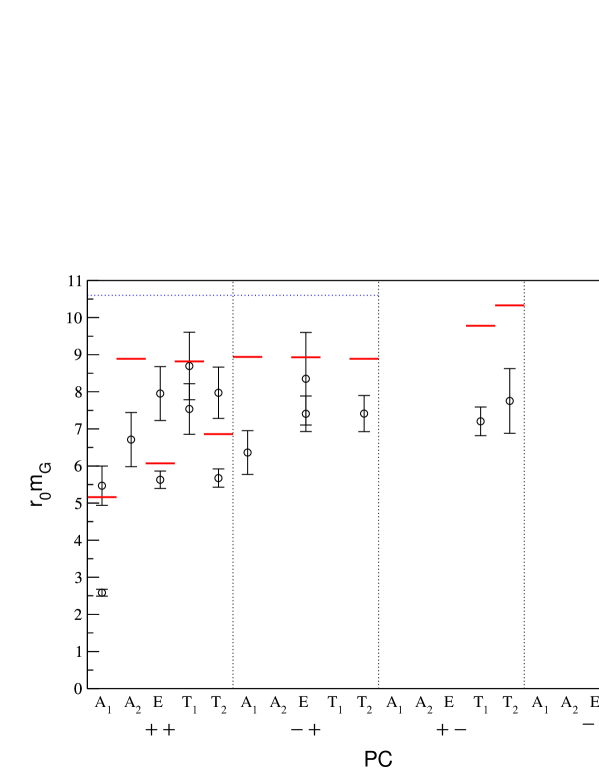
Figure 6.16: The results of the glueball measurements at $\beta=3.15$ converted into units of $r_{0}$. The lower bounds of the energies of multi-glueball states (solid lines) or torelon pairs (dotted line) are given as well.

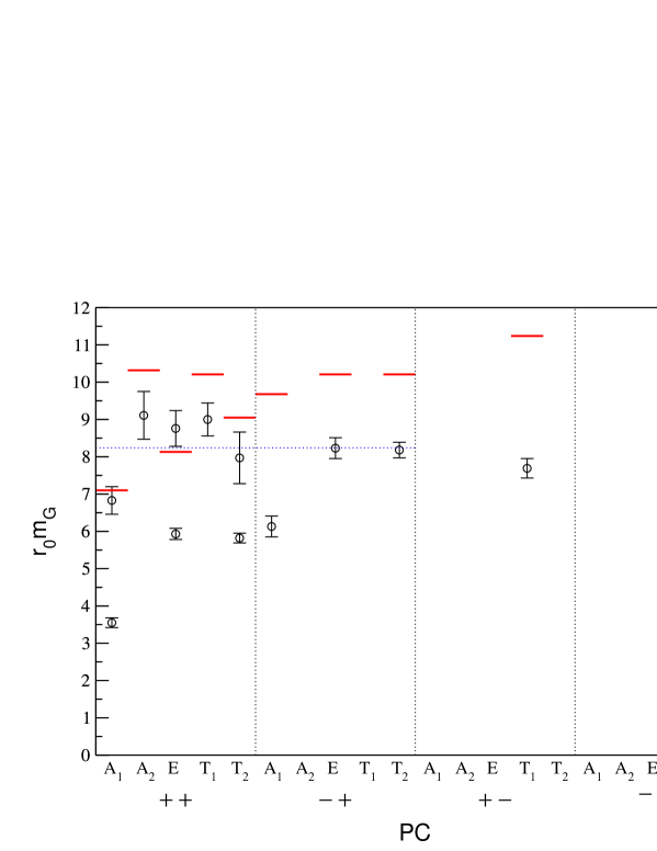
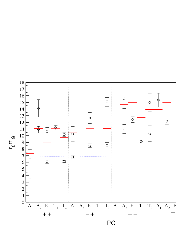
Figure 6.17: The results of the glueball measurements at $\beta=3.30$ converted into units of $r_{0}$. The lower bounds of the energies of multi-glueball states (solid lines) or torelon pairs (dotted line) are given as well.

Figure 6.18: The results of the glueball measurements at $\beta=3.50$ converted into units of $r_{0}$. The lower bounds of the energies of multi-glueball states (solid lines) or torelon pairs (dotted line) are given as well.

6.5.4 The Continuum Limit

In order to remove discretisation errors from glueball masses $r_{0}m_{G}$ that have been obtained on lattices with finite lattice spacing, we have to perform the continuum limit, i.e. to extrapolate the results to $a_{s}=0$. Having obtained results at three values of the coupling $\beta$, one of them corresponding to rather coarse lattices, and having no accurate information (e.g. from perturbation theory) about the behaviour of the energies depending on the lattice spacing (about the form of the curve used in the extrapolation) this is not an easy task and rather ambiguous.

We perform two different kinds of continuum limits. Firstly, we extrapolate the masses in terms of the hadronic scale $r_{0}$, $r_{0}m_{G}=m_{G}a_{t}\cdot\xi\cdot r_{0}/a_{s}$, secondly, we extrapolate mass ratios $m_{G_{1}}/m_{G_{2}}$ of different glueball representations. Generally, the procedure we resort to, is the following: We include all the three energies or mass ratios, obtained at $\beta=3.15,3.30,3.50$, into the fit and use the form

$$r_{0}m_{G}\mid_{a_{s}}=r_{0}m_{G}\mid_{a_{s}=0}+c_{2}\left(\frac{a_{s}}{r_{0}}\right)^{2}.$$ (6.5)

Additionally, we perform fits including only the results from the two finer lattices at $\beta=3.30,3.50$ using a constant (if this fits the results reasonably well) or the form stated above. This value of the continuum mass (or mass ratio) is then compared to the result of the fit of all the three data points, which is only accepted if the two results coincide within their errors.

Masses in Terms of $\mathbf{r_{0}}$

For the extrapolation of masses in terms of the hadronic scale $r_{0}$, this procedure works very well for the representations $A_{2}^{++}$, $E^{-+}$, $E^{++}$, ${E^{++}}^{*}$, $T_{2}^{-+}$ and $T_{2}^{++}$ where we may always fit the results from the two finer lattices to a constant which agrees with the result of the extrapolation using eq. 6.5 on all three data points. For the $A_{1}^{-+}$ representation, we obtain the best results fitting the masses to a constant, for the fit to two data points as well as to three data points.

Much more difficult is the extrapolation for the scalar glueball and its excited state, $A_{1}^{++}$ and ${A_{1}^{++}}^{*}$. It turns out that the fit has a very bad $\chi^{2}$ and describes the data very badly if eq. 6.5 is used. However, we find good behaviour if we use

$$r_{0}m_{G}\mid_{a_{s}}=r_{0}m_{G}\mid_{a_{s}=0}+c_{6}\left(\frac{a_{s}}{r_{0}}\right)^{6}$$ (6.6)

for the ground state as well as for the excited state energies and thus decide to use this (ad-hoc) fitting form for the scalar glueball. The results of the continuum extrapolations for various glueball states are collected in Table G.14. In Figures 6.19, 6.20 the curves are shown together with the measured values for the $PC=++$ and the $PC=-+$ sectors where extrapolations are possible with the present data.

Other representations where energies can be determined at several values of $\beta$, such as $T_{1}^{+-}$, $T_{1}^{++}$ or ${T_{2}^{++}}^{*}$ do not yield consistent results using the procedure presented above and we decide to abstain from performing continuum extrapolations in terms of $r_{0}m_{G}$ for these states.

Mass Ratios

The other method of extrapolating to the continuum, namely using mass ratios $m_{G_{1}}/m_{G_{2}}$ between different glueball representations, has got the advantage that uncertainties present in the determination of $r_{0}/a_{s}$ or the renormalised anisotropy $\xi_{R}$ do not enter into the continuum extrapolation. Furthermore, we may assume that several effects such as finite size scaling are more similar for different glueball states measured on the same lattice as opposed to completely different quantities such as the static quark-antiquark potential or the torelon dispersion relation measured on different sized lattices that are used to obtain $r_{0}/a_{s}$ and $\xi_{R}$, respectively.

The common way of extrapolating glueball mass ratios to the continuum is using ratios $m_{G}/m_{0^{++}}$ (see Table G.12), i.e. ratios to the scalar glueball mass, which is the lightest mass present. Doing this, we observe that the extrapolation is difficult, the goodness of the fit is rather bad and the errors are large. Furthermore, the resulting continuum mass ratios are not in good agreement to ratios of the continuum masses coming from the extrapolation of the masses in terms of $r_{0}$. This is not a surprise, because the behaviour of the scalar glueball as a function of the lattice spacing is rather difficult, i.e. there are large cut-off effects that cannot be described too easily. Additionally, the errors of the mass estimates of the scalar glueball are quite large. Due to these reasons, we decide to use the well measured masses of the tensor $T_{2}^{++}$ representation, which show small errors and seem to scale rather well. These ratios are listed in Table G.13.

The procedure of the extrapolation is the same as for the case of $r_{0}m_{G}$ described in the previous section; the unambiguous results are listed in Table G.15. Again, for the $A_{1}^{-+}$ states, as well as for the $E^{++}$, the fit to a constant works out best; the $T_{2}^{-+}$ glueball can only be reasonably extrapolated using a fitting form analogous to eq. 6.6. Note, that this way we obtain continuum results for the representations $T_{1}^{+-}$, $T_{1}^{++}$ and ${T_{2}^{++}}^{*}$ which is not possible performing the extrapolation using masses in terms of $r_{0}$. Furthermore, all the other results listed are in agreement to the ratios of the continuum masses $r_{0}m_{G}$ within one standard deviation.

In the following, we will use the finite lattice spacing results from the simulation on the finest lattice at $\beta=3.50$ for the energies of states that cannot be extrapolated to the continuum in one of the two ways, e.g. to study degeneracies or to draw a (rather qualitative) picture of the low-lying glueball spectrum. In tables listing continuum results, these values not extrapolated to $a_{s}=0$ will be stated in square brackets.

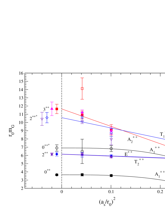
Figure 6.19: Mass estimates of the $PC=++$ glueballs in terms of the hadronic scale $r_{0}$ against $(a_{s}/r_{0})^{2}$. The curves are the continuum limit extrapolations of the form $r_{0}m_{G}+c_{2}(a_{s}/r_{0})^{2}$. Circles: $A_{1}^{++}$, boxes: $A_{2}^{++}$, diamonds: $E^{++}$, upward triangles: $T_{1}^{++}$, downward triangles: $T_{2}^{++}$; solid symbols: ground states, open symbols: first excited states. Note that the continuum results of the representations $T_{1}^{++}$ and ${T_{2}^{++}}^{*}$ have been obtained using a fit of glueball mass ratios.

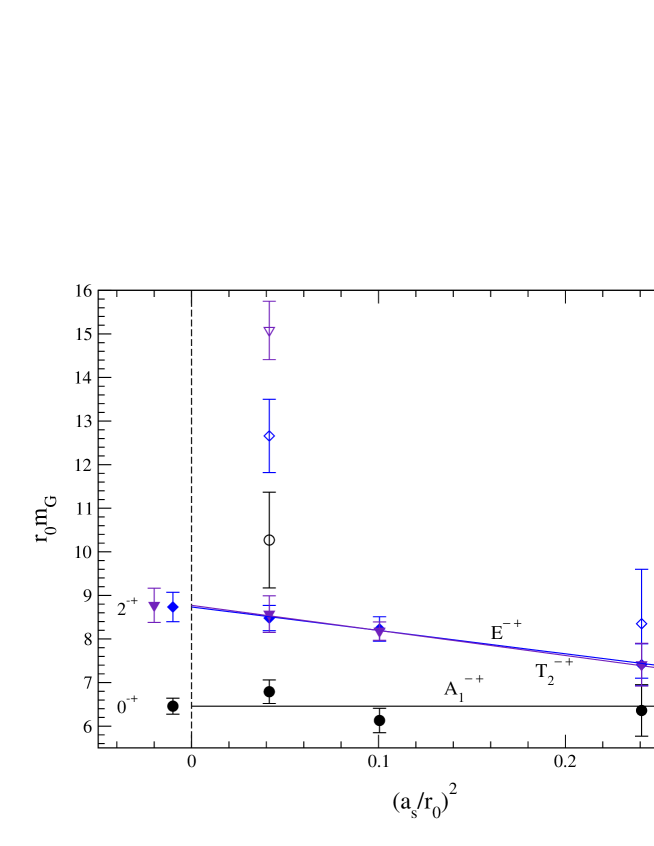
Figure 6.20: Mass estimates of the $PC=-+$ glueballs in terms of the hadronic scale $r_{0}$ against $(a_{s}/r_{0})^{2}$. The curves are the continuum limit extrapolations of the form $r_{0}m_{G}+c_{2}(a_{s}/r_{0})^{2}$. Circles: $A_{1}^{-+}$, diamonds: $E^{-+}$, downward triangles: $T_{2}^{-+}$; solid symbols: ground states, open symbols: first excited states.

6.5.5 Continuum Spin Identification

Once the extrapolation of the measured glueball energies to the continuum, $a_{s}=0$, has been performed, what remains is the assignment of continuum spin $J$ to the different representations of the cubic group $\Gamma$. From Table 2.2 we know from which lattice representations $\Gamma^{PC}$ a continuum glueball with quantum numbers $J^{PC}$ may obtain contributions, where the assignment of parity $P$ and charge conjugation $C$ is simply $1:1$. Degeneracies (in the continuum limit) between several representations $\Gamma^{PC}$ contributing to the same continuum state $J^{PC}$ are a strong indication for the correctness of the assignment of all the lattice states involved to the same continuum $J^{PC}$ glueball. Furthermore, we make the assumption that the mass of the glueballs increases with the spin getting larger.

In the $PC=++$ sector, we observe a single low-lying state, $A_{1}^{++}$, which is thus assigned $J=0$. The $E^{++}$ and $T_{2}^{++}$ states are degenerate to a very high precision as it should happen if these representations correspond to the five polarisations of a $J=2$ glueball. The excited state ${A_{1}^{++}}^{*}$ again has no degenerate partner and is assigned to an excited state of the continuum $J=0$ glueball. The excited states ${E^{++}}^{*}$ and ${T_{2}^{++}}^{*}$ again turn out to be degenerate and so they are assigned to an excitation of the $J=2$ glueball. The same situation is met with the representations $A_{2}^{++}$ and $T_{1}^{++}$ which are thus assigned $J=3$. The first excitation ${T_{2}^{++}}^{*}$ being part of the $J=2$ state, the missing 3 polarisations should come from the second excitation of $T_{2}^{++}$ which cannot be measured by our simulations.

In the $PC=-+$ sector, the situation of the $A_{1}^{-+}$ and the $E^{-+}$ and $T_{2}^{-+}$ is very similar to the one of their partners in the $PC=++$ sector; these states are thus assigned $J=0$ and $J=2$ respectively. The remaining three, excited states have no apparent degeneracies, there is thus no safe assignment of continuum spin to these states. The facts that the excited state ${A_{1}^{-+}}^{*}$ is rather light and comes with no degenerate partner, raises the presumption that it is the excited $J=0^{-+}$ glueball.

In the other two sectors, continuum extrapolations of our measured energies are not possible, except for the representation $T_{1}^{+-}$ using mass ratios. However, looking at the degenerate representations in the $PC=++,-+$ sectors, it is noticeable that the degeneracies are apparent even for finite lattice spacing at $\beta=3.50,3.30$. Assuming that this behaviour persists for $PC=+-,--$, at least for energies not too high, we may assign continuum spin even to some of the remaining states.

In the $PC=+-$ sector, we notice the lowest-lying $T_{1}^{+-}$ state which has no degenerate partner which suggests a $J=1$ interpretation. Next, there is the $A_{2}^{+-}$ which is likely to correspond to $J=3$.

Finally, in the $PC=--$ sector, there are different possible scenarios. The almost exact degeneracy of $T_{1}^{--}$ and $T_{2}^{--}$ suggests them contributing to the $J=3$ continuum state. The rather heavier state $A_{2}^{--}$ could still be degenerate with the two latter states (note the high mass and the finite lattice spacing!) and carry the remaining polarisation. Admittedly, it could as well correspond to an excited $J=3$ state or even to $J=6$. The final $A_{1}^{--}$ state is very heavy and indicates that glueballs with even spin and $PC=--$ have large energies as the representation $A_{1}$ contributes solely to even numbered spin states up to $J=8$!

The rather well supported continuum spin assignments presented above are given together with the glueball masses in Tables 6.9, G.14, G.15, the final results on the masses of these states are collected, together with the masses in MeV, in Table 6.11. Figure 6.21 provides a rather qualitative picture of the low-lying glueball spectrum as obtained from our $\xi=2$ simulations.

$J^{PC}$	$\Gamma^{PC}$	$m_{G}r_{0}$	$m_{G}$ [MeV]
$0^{++}$	$A_{1}^{++}$	3.64(10)	1440(40)
${0^{++}}^{*}$	${A_{1}^{++}}^{*}$	6.90(38)	2730(150)
$2^{++}$	$E^{++}$, $T_{2}^{++}$	6.15(15)	2430(60)
${2^{++}}^{*}$	${E^{++}}^{*}$, ${T_{2}^{++}}^{*}$	10.52(51)	4160(200)
${3^{++}}$	$A_{2}^{++}$, $T_{1}^{++}$	11.65(49)	4600(190)
${0^{-+}}$	$A_{1}^{-+}$	6.46(18)	2550(70)
${2^{-+}}$	$E^{-+}$, $T_{2}^{-+}$	8.75(26)	3460(110)
${0^{-+}}^{*}$	${A_{1}^{-+}}^{*}$	[10.27(110)]	[4060(430)]
${1^{+-}}$	$T_{1}^{+-}$	9.45(71)	3730(280)
${3^{+-}}$	$A_{2}^{+-}$	[11.02(68)]	[4350(270)]

Table 6.11: Final results for the masses of continuum glueballs with quantum numbers $J^{PC}$, obtained from the lattice representations $\Gamma^{PC}$. For the conversion to MeV, $r_{0}^{-1}\approx 0.5$ fm $\approx 395$ MeV has been used. Quantities in brackets have not been extrapolated to the continuum but denote results from the simulation on the finest lattice at $\beta=3.50$ (corresponding to $a_{s}=0.102$ fm).

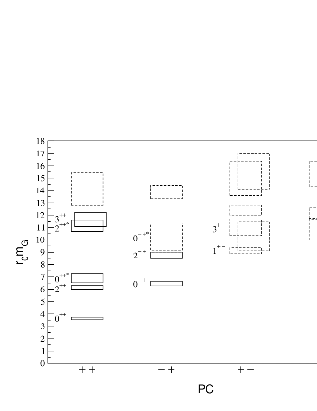
Figure 6.21: The mass spectrum of glueballs in SU(3) pure gauge theory as obtained from our simulations using the $\xi=2$ classically perfect action. The masses are given in units of the hadronic scale $r_{0}$. The dashed boxes are used for states that could not be extrapolated to the continuum, instead the mass obtained from the simulation on the finest lattice at $\beta=3.50$ is given. The most probable assignment of continuum spin is indicated as well.

6.5.6 Discussion

In order to discuss the results obtained from the glueball measurements, presented in the previous Sections, let us first list the sources of errors that may be present. Firstly, there are finite size effects; our finest lattice ($\beta=3.50$) has got a spatial volume of (1.22 fm)³ which is rather small compared to other volumes used in glueball measurements. The magnitude of finite-size effects depends largely on the quantity studied, more precisely on the form of the glueball wavefunctions (above all their extension). Due to the three volumes employed having such different size, finite-size effects do not only systematically shift the lattice results but they can also make reliable continuum extrapolations much more difficult or even impossible.

Secondly, the mass of the scalar glueball $A_{1}^{++}$ (above all the ground state) shows very large cut-off effects. These could be due to the presence of a critical end point of a line of phase transitions in the fundamental-adjoint coupling plane assumed to define the continuum limit of a scalar field theory. Our action includes in its rich structure operators transforming in the adjoint representation. If their net coupling (which we do not control during the construction and the parametrisation of the action) lies in a certain region, the effect of the critical end-point on scalar quantities at certain lattice spacings (sometimes called the “scalar dip”) may even be enhanced compared to other (more standard) discretisations with purely fundamental operators.

Furthermore, our analysis shows that states consisting of several glueballs or torelon pairs could mix with most of the higher-lying states occurring in our measurements. This makes the interpretation of the measured states more difficult, additionally, systematic effects (e.g. different mass shifts at different values of $\beta$ because of the different lattice sizes or due to the presence of operators having larger overlap with unwanted states) may again complicate the continuum extrapolation.

Finally, as always, there is the statistical error. Generally, it does not introduce bias and it can be estimated quite reliably. However, glueball correlators are notorious for large statistical noise and this noise may hamper the reliable variational analysis of states that in principle could still be measured as for their energies.

There are several possibilities of improving the measurements. Firstly, and most simple, improving the statistics may help. This can be seen e.g. looking at the results of the simulation on the coarsest lattice at $\beta=3.15$. Although the lattice is coarser, more energies can be determined than on the finer $\beta=3.3$-lattice, mainly due to the larger statistics. Additionally, a lot of problems stated previously are solved (or at least kept under control) if for each value of $\beta$, we determine the glueball energies on several lattices of different physical size. Studying the finite-size scaling creates the possibility of separating single glueball from other (multi-glueball, torelon pair) states and it provides estimates of finite lattice spacing infinite-volume results to be used in a safe continuum extrapolation. Another way of improving the measurements is systematically studying the operators employed to create and annihilate single glueball states in order to increase their overlap with the single glueballs to be measured and to decrease their overlap with all the other states. This includes the study of other smearing techniques, such as e.g. Teper fuzzing [147]. Conversely, the introduction of operators coupling most strongly to the unwanted multi-glueball or torelon-pair states allows for the calculation of mixing strengths in order to exclude all the unwanted states from further analysis. Another technically rather easy but computationally expensive way of improving the results is performing simulations on additional values of $\beta$. This allows for a more detailed study of the continuum limit, especially in the case of non-perturbatively improved actions, where there is no clearcut information about the way how the continuum is approached. Naturally, one has to take care not to go too deep into the strong coupling region as there is not much information about the continuum; performing simulations on two additional values of $\beta$ corresponding to $(a_{s}/r_{0})^{2}\approx 0.16,0.3$ would probably be a good choice in our case. But keep in mind that for each additional lattice spacing the measurements of the torelon dispersion relation as well as of the static-quark potential have to be repeated.

There is one error which is not cured by the measures recommended in the last paragraph, namely the effects on the scalar states, coming from the “scalar dip”. Morningstar and Peardon improve the situation adding a two-plaquette adjoint term with a negative coefficient which results in an approach to the continuum on a trajectory always far away of the dangerous “dip” region [19]. In principle, the classically perfect action could be treated the same way: Extract all the operators with adjoint contributions present in the parametrisation, determine their sign and add another (non-linear) constraint to the fit, namely that the action of all these operators together corresponds to an adjoint operator with a certain (negative) coupling. Because of the large freedom in the fit, the inclusion of this single criterion should not impair the quality of the parametrisation considerably.

Collab.	$r_{0}m_{0^{++}}$	$r_{0}m_{2^{++}}$
UKQCD [107]	4.05(16)	5.84(18)
Teper [137]	4.35(11)	6.18(21)
GF11 [138]	4.33(10)	6.04(18)
M&P [18]	4.21(15)	5.85(8)
Liu [20]	4.23(22)	5.85(23)
FP action	4.12(21)	[5.96(24)]
AICP	3.64(10)	6.15(15)

Table 6.12: Comparison of the lowest-lying glueball masses in units of $r_{0}$. Values in brackets denote masses obtained at a lattice spacing $a=0.10$ fm and are not extrapolated to the continuum.

Collab.	$r_{0}m_{0^{-+}}$	$r_{0}m_{{0^{++}}^{*}}$	$r_{0}m_{2^{-+}}$	$r_{0}m_{1^{+-}}$
Teper [137]	5.94(68)	7.86(50)	8.42(78)	7.84(62)
M&P [18]	6.33(13)	6.50(51)	7.55(11)	7.18(11)
FP action	[6.74(42)]		[8.00(35)]	[7.93(78)]
AICP	6.46(18)	6.90(38)	8.75(26)	9.45(71)

Table 6.13: Comparison of glueball masses in units of $r_{0}$. Values in brackets denote masses obtained at a lattice spacing $a=0.10$ fm and are not extrapolated to the continuum.

Table 6.12 compares the newly obtained continuum glueball masses with the result of the isotropic FP action as well as with results obtained by other collaborations. There is reasonable agreement between the different determinations of the $2^{++}$, ${0^{++}}^{*}$, $0^{-+}$, $2^{-+}$ glueball masses. The situation for the scalar $0^{++}$ and for the $1^{+-}$ state is different, however. The scalar glueball mass comes out about 5 standard deviations below the average mass of the other collaborations if only the usual statistical errors are considered. Thinking of all the possible sources of errors stated above, which are (partly) also present in the analyses of the other groups, we tend to explain this discrepancy with underestimated (or disregarded) errors. Concerning the $1^{+-}$ glueball, looking at the masses determined on the lattices ($T_{1}^{+-}$ in Table 6.9), we observe that the masses determined on the coarser (and larger) lattices at $\beta=3.15,3.30$ coincide with the (continuum) results obtained by other groups and do not even show a significant discrepancy, despite the considerable difference between the lattice spacings. The mass determined on the fine (and small) lattice at $\beta=3.50$ however, is much higher. This tendency is even amplified by the continuum extrapolation. We suspect that this state exhibits strong finite-size effects pushing up its mass in small volumes.

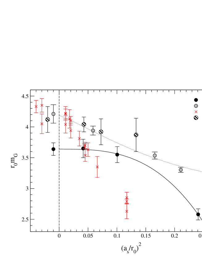
Figure 6.22: Lattice results for the scalar ($0^{++}$) glueball mass, together with results of continuum extrapolations obtained from simulations employing different actions. The different continuum values for the Wilson action stem from different groups.

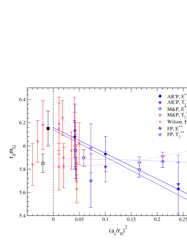
Figure 6.23: Lattice results for the tensor ($2^{++}$) glueball mass, together with results of continuum extrapolations obtained from simulations employing different actions. The continuum extrapolations of the $E^{++}$ and $T_{2}^{++}$ representations are averaged in order to get the mass of the single continuum glueball. The different continuum values for the Wilson action stem from different groups.

Figures 6.22 and 6.23 compare our measurements of the $A_{1}^{++}$, $E^{++}$ and $T_{2}^{++}$ states to measurements obtained by other groups, using different actions, as well as to the isotropic FP action results. Concerning the scalar glueball, the artifacts at moderate lattice spacings corresponding to $(a_{s}/r_{0})^{2}\lesssim 0.15$ ($a_{s}\lesssim 0.19$ fm) seem to be rather smaller for the isotropic FP as well as for the anisotropic classically perfect action compared to the tadpole and treelevel improved action (M&P) and certainly much smaller than the artifacts of the Wilson action. The mass obtained on the coarsest lattice at $\beta=3.15$ (corresponding to $a_{s}\approx 0.24$ fm) using the classically perfect anisotropic action (AICP), however, exhibits large cut-off effects of about 30% (compared to about 20% for the M&P action), probably due to the scalar dip. Concerning the tensor glueball, the picture is not clear, mainly due to the considerable statistical errors of the measurements, except of the ones obtained by using the tadpole and treelevel improved anisotropic action.

These considerations show again, that in order to obtain fool-proof results measuring glueball masses (and other quantities) on the lattice, one has to make sure to measure everything that is necessary, taking into account a certain number of lattices with different couplings $\beta$, lattices with different volumes, measuring the renormalised anisotropy for all the values of $\beta$ considered and measuring additional operators having large overlaps with states that could mix.

Being the first application of the FP action technique to anisotropic gauge theory, it goes beyond the scope of this work to check all the possible sources of errors in the glueball mass determinations. Observing the difficulties arising with the determination of the glueball spectrum already in pure gauge theory, one can estimate that reliable determinations in the context of more and more unquenched Lattice QCD (including lighter and lighter dynamical fermions until, finally, one ends up with quarks having their natural mass) will be a very tough job. However, this will yield information about the fate of glueballs in the presence of quarks and possibly solve the big puzzle concerning the presence (or absence) of glueballs in nature. It will thus be really worth the big effort.

Chapter 7 Repeating the Spatial Blocking Step

As noted in Chapter 4, the spatial blocking step used to obtain a classically perfect $\xi=2$ action may be repeated straightforwardly to obtain actions with higher anisotropies. Using another spatial scale 2 blocking step we create a classically perfect $\xi=4$ gauge action and parametrise it the same way as the $\xi=2$ action. Furthermore, we measure the renormalised anisotropy and show that it is indeed feasible to construct such actions to be used in MC simulations for heavy states such as glueballs. The classically perfect $\xi=4$ action is not yet examined thoroughly, however the parametrisation is ready (see Appendix D.6) and the analyses of the $\xi=2$ action (see Chapter 6) may be repeated for $\xi=4$.

7.1 Perfect Actions for Larger Anisotropies

Each application of the spatial blocking step (slightly) renormalises the anisotropy of the action; the renormalised anisotropies of the final actions thus have to be measured in the end. However, this is necessary anyhow if one is interested in comparing results (other than e.g. mass ratios, where the renormalisation of the anisotropy cancels out) to other collaborations or to the experiment.

In order to be able to repeat the spatial blocking step getting from $\xi=2$ to $\xi=4$ we construct a $\xi=2$ action which is valid on minimised $\xi=4$ configurations including into the fit configurations at different values of $\beta$ covering a large range. The $\xi=2$ action presented in Chapter 6 is not suitable for this task as it is dedicated to be used solely on largely fluctuating configurations around $\beta=3.0$. The construction and the parameters of the intermediate $\xi=2$ action are described in Appendix D.5.

Once the fine action to be used on the r.h.s. of the renormalisation group equation, eq. 1.5, is ready, we may proceed the same way as for the $\xi=2$ action. We perform the non-linear fit on 2 $\xi_{\text{ad-hoc}}=6$ configurations each at $\beta_{\text{ad-hoc}}=$ 4.0, 3.5, 3.0, 2.5, 2.0. It turns out that in order to obtain parametrisations that are free of dangerous “traps” in the $u$-$w$ plane (see Section 1.4.5) we have to include the condition $\mathcal{A}(u,w)>0$ at ten points $(u,w)$ into the non-linear fit. Studying the values of $\chi^{2}$ as well as the linear behaviour of the parametrisations we decide to use a set with $\max(k+l)_{\text{sp}}=3$, $\max(k+l)_{\text{tm}}=2$. The parameters are given in Appendix D.6, the behaviour of the linear parameters is displayed in Figure 1.5.

7.2 The Renormalised Anisotropy

To check whether the construction of the classically perfect $\xi=4$ action worked well and whether the parametrisation reproduces the input anisotropy, we measure the renormalised anisotropy at one value of $\beta=3.0$, using the torelon dispersion relation, following the method described in Sections 2.1 and 6.2. The simulation parameters are collected in Table 7.1.

$\beta$	$S^{2}\times L\times T$	# sweeps / measurements
3.0	$8^{2}\times 4\times 32$	54000 / 10800

Table 7.1: Run parameters for the torelon measurements using the $\xi=4$ perfect action. The lattice extension in torelon direction $L$, the extension in the two transversal spatial directions $S$ as well as the temporal extension $L$ are given.

Due to the (expected) coarser spatial lattice spacing we do not need as many smearing steps as for the $\xi=2$ action and thus perform our measurements on configurations of smearing levels 2, 4, 6, 8, 10 keeping $\lambda_{s}=0.1$ fixed.

Figure 7.1 displays the dispersion relation obtained, in Table G.16 the measured energies $E(p^{2})$ determined using variational methods (see Appendix E) depending on the lattice momentum $p^{2}$ are given, together with the number of operators used in the variational method, the fit ranges and the values of $\chi^{2}$ per degree of freedom, $\chi^{2}/N_{\text{DF}}$. The renormalised anisotropy as well as the torelon mass are determined in exactly the same way as for the $\xi=2$ action. The results are listed in Table 7.2. Furthermore, we may again evaluate an estimate of the lattice scale using the string picture relation, eq. 6.1, yielding $\sqrt{\sigma}a_{s}=0.532(16)$, and thus $r_{0}/a_{s}=2.241(86)$ which corresponds to $a_{s}=0.22$ fm, $a_{t}=0.060$ fm. Having a torelon of length $La_{s}\approx 0.89$ fm the error of the scale estimate is expected to be of about 5-10% (see Table 6.4).

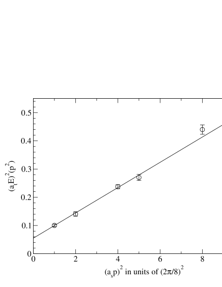
Figure 7.1: Torelon dispersion relation for $\beta=3.0$. The straight line is the correlated fit to $E^{2}(p)=m_{T}^{2}+p^{2}$ in the range $p^{2}=1..5$.

$\beta$	fit range	$\xi_{R}$	$m_{\text{T}}a_{t}$	$\chi^{2}/N_{\text{DF}}$
3.0	1..5	3.71(8)	0.235(13)	0.82

Table 7.2: Results of the torelon simulations using the “$\xi=4$” perfect action. The fit range in $p^{2}$ is given in units of $(2\pi/S)^{2}$.

Concerning the application of the spatial blocking method presented in this work to yield classically perfect gauge actions for higher anisotropies, we may conclude that the construction including the blocking as well as the parametrisation works in exactly the same way as the construction of the $\xi=2$ action to which the main body of this work is dedicated. The resulting action shows a renormalisation of the anisotropy of about 7% at the value of $\beta=3.00$ where this has been measured. Calculations of physical observables such as the static quark-antiquark potential or glueball masses using the $\xi=4$ action are still absent.

Chapter 8 Properties of the Perfect Anisotropic Actions

In this Chapter, we examine the autocorrelation times and the average change of the gauge links for different updates in the MC simulation for anisotropies $\xi=1,2,4$. Furthermore, the computational overhead of the parametrisation of the perfect action is compared to the standard Wilson action as well as to the widely-used Symanzik and tadpole improved anisotropic action.

8.1 Updating Algorithms

There are different methods of updating Monte Carlo (MC) configurations. The two methods we use for our rather complex parametrised gauge actions are the plain local Metropolis algorithm as well as pseudo over-relaxation (POR), both described in the next two sections.

In order to define the run parameters of MC simulations one should know about the properties of the updates, in order to have configurations that have small autocorrelation, to be sure that the algorithm does not introduce any bias and to estimate the optimal MC time between measurements of observables.

8.1.1 Local Metropolis Update

A very general method for updating MC ensembles satisfying detailed balance has been introduced by Metropolis et al. [148]. We update link by link, first proposing a new link $U^{\prime}\in$ SU(3). The change $U\rightarrow U^{\prime}$ is accepted with probability 1 if the action of the proposed configuration is smaller than the initial action, with probability $e^{-\Delta S}$ if the action increases with the update. In our updating procedure we use proposed links $U^{\prime}$ that are products of the initial link $U$ and random SU(3) matrices whose fluctuations are chosen such that the acceptance rate of the Metropolis sweep stays between 0.3 and 0.7.

There is the possibility of performing multi-hit updates, i.e. using “coarser” trial matrices that lead to larger changes and compensating for the lower acceptance by trying several proposed links in a row.

8.1.2 Pseudo Over-Relaxation Update

The method of over-relaxation bases on the fact that for simple actions (as e.g. the Wilson gauge action) it is possible to perform large changes in the update of a link without changing the action $S$, i.e. to perform micro-canonical updates. For SU(3) gauge theory this may be done executing such updates subsequently on different SU(2) subgroups.

For our complex parametrisation, exact micro-canonical steps are not easy to implement. That is why we propose new links that would not change the corresponding part of the anisotropic Wilson action and correct for the change in the perfect action by adding an accept-/reject step, i.e. our pseudo over-relaxation (POR) algorithm is a variant of the Metropolis algorithm presented in the last Section, where the generation of the proposed links is altered. However, one has to be careful about this procedure because all the configurations that are reached by subsequent POR updates lie on the same $\mathcal{A}_{\text{Wilson}}=\text{const}.$ hyperplane in configuration space. In order to keep ergodicity, POR steps have to be mixed with another kind of (ergodic) updates, e.g. with Metropolis steps. Additionally, due to the similarities of the Wilson action and the FP action, during the thermalisation, when a certain action level shall be reached, it may be favourable to use rather less POR steps than later on, generating configurations at the same coupling $\beta$.

8.2 The Autocorrelation

The autocorrelation is a measure of correlation between an observable with the very same observable at a later (MC) time. Near phase transitions, the autocorrelations in MC simulations of observables are proportional to a power $n$ of the lattice correlation length $\xi^{\text{lat}}$:

$$\tau_{\text{op}}\sim(\xi^{\text{lat}})^{n},$$ (8.1)

where theoretically $n=2$ for local stochastic (Metropolis) and $n=0$ for cluster or over-relaxation updates. Eq. 8.1 shows as well that one has to expect critical slowing down, i.e. a dramatic increase of the autocorrelation time, if one simulates near a phase transition with divergent correlation length $\xi$ using local stochastic updates only.

On the anisotropic lattice there are two different correlation lengths (in lattice units) $\xi^{\text{lat}}_{s}$ in spatial and $\xi^{\text{lat}}_{t}$ in temporal direction, where $\xi^{\text{lat}}_{s}/\xi^{\text{lat}}_{t}=a_{t}/a_{s}=\xi^{-1}$ (where this latter $\xi$ denotes the anisotropy).

Operators that couple strongly to $\xi^{\text{lat}}_{t}$, i.e. operators living in the spatial domain, are thus expected to have autocorrelation times rising with the anisotropy for simulations that are performed not too far away from phase transitions.

8.2.1 The Integrated Autocorrelation Time

Let us first introduce the (unnormalised) autocorrelation function of an operator $O$, $C_{OO}(t)$:

$$C_{OO}(t)=\langle O(\tau)O(\tau+t)\rangle-\langle O\rangle^{2}.$$ (8.2)

As well, we define the normalised autocorrelation function $\rho(t)$:

$$\rho_{OO}(t)=\frac{C_{OO}(t)}{C_{OO}(0)}.$$ (8.3)

Typically, $\rho(t)$ decays exponentially, $\rho(t)\sim\exp(-|t|/\tau)$ for $|t|$ large enough and we thus define the exponential autocorrelation time $\tau_{\text{exp}}$

$$\tau_{\text{exp},O}\equiv\lim_{t\rightarrow\infty}\frac{t}{-\ln|\rho_{OO}(t)|},$$ (8.4)

which is the “lifetime” of the correlation. This definition is vivid, however what is more important for the statistics of MC runs is the integrated autocorrelation time $\tau_{\text{int}}$ which is describing the loss of statistics due to the subsequent configurations not being completely independent:

$$\text{var}(\bar{O})\approx\frac{1}{n}(2\tau_{\text{int},O})C(0),$$ (8.5)

i.e. the true variance of the estimated observable $O$ is a factor $2\tau_{\text{int},O}$ larger than if the configurations were completely independent of each other.

There are different possibilities of estimating $\tau_{\text{int}}$. Firstly, there is an inequation between the two autocorrelation times [149, 150, 151] which holds for algorithms that satisfy detailed balance:

$$\tau_{\text{int}}\leq\frac{1}{2}\left(\frac{1+e^{-1/\tau_{\text{exp}}}}{1-e^{-1/\tau_{\text{exp}}}}\right)\approx\tau_{\text{exp}}.$$ (8.6)

The exponential autocorrelation time $\tau_{\text{exp}}$ can be obtained performing fits to $\rho(r)$. For a direct estimate of $\tau_{\text{int}}$ on may use the same procedure as used by the QCD-TARO collaboration in [152], where

$$\tau_{\text{int}}=\frac{1}{2}\rho(0)+\sum_{t=1}^{N}\rho(t)\frac{N-t}{N},$$ (8.7)

where $N$ is determined such that $\tau_{\text{int}}$ is maximised, at the same time $N<10$ % of the total sample.

Another method has been proposed by Sokal in [150, 151]:

$$\tau_{\text{int}}=\frac{1}{2}\sum_{t=-m}^{m}\frac{R(t)}{R(0)},$$ (8.8)

with

$$R(t)=\frac{1}{n-|t|}\sum_{i=1}^{n-|t|}(O_{i}-\bar{O})(O_{i+|t|}-\bar{O}),$$ (8.9)

where $n$ is the number of measurements performed (extent of “MC time”). The parameter $m$ defines a “window” in which the measurements are taken into account to calculate the integrated autocorrelation time. The corresponding variance of the estimate is

$$\text{var}(\tau_{\text{int}})\approx\frac{2(2m+1)}{n}\tau_{\text{int}}^{2}$$ (8.10)

for $\tau\ll m\ll n$. There are several possibilities choosing $m$; generally, large $m$ leads to a small bias of the estimated $\tau_{\text{int}}$, however, the variance is growing with increasing $m$. One possibility is to fix $m=c\tau_{\text{int}}$ with a factor $c$ depending on the behaviour of $\rho(t)$ ($c\approx 4$ for purely exponential decay, $c\approx 6$ for asymptotic or pre-asymptotic decays or even $c\approx 10\sim 20$ for exceptionally slow decays). However, analogous to the procedure described before, we choose $m$ such that the estimate for $\tau_{\text{int}}$ is maximised. It turns out, that there is always a long plateau of maximal $\tau_{\text{int}}$ and that the bias corresponding to the $m$ chosen is small. That is why we display the resulting values of the integrated autocorrelation time together with their standard deviation.

In practice, the effect of autocorrelations of the operators between measurements close in the MC trajectory is taken into account by binning subsequent measurements into blocks of length $T_{\text{MC}}>\tau_{\text{int}}$, where $\tau_{\text{int}}$ should be the largest integrated autocorrelation time of the operators measured in the simulation. These binned measurements are independent from each other and yield the correct variance of the observables, if they are used e.g. in a bootstrap procedure.

8.3 The Change in the Update

A measure for the change of the configuration in a sweep is the following

$$(\Delta U)_{\text{upd}}=\frac{1}{N_{\text{upd}}}\sum_{i=1}^{N_{\text{upd}}}[N_{c}-\text{Re Tr}(U_{i}U_{i}^{{}^{\prime}\dagger})],$$ (8.11)

which is the average change per gauge link in one update; $N_{\text{upd}}$ is the number of update attempts, $U$ and $U^{\prime}$ denote the initial and the updated link respectively (of course $U^{\prime}\equiv U$ for rejected steps). It is this change that is expected to be considerably larger for (pseudo) over-relaxation updates compared to standard Metropolis steps.

The measure defined above may also be used as a measure for autocorrelations of the most local objects, i.e. the gauge links itself, if it is used to compare an initial configuration ($U$) to the configurations at MC time $t=1,2,3,\ldots$ ($U^{\prime}$).

8.4 Results

To study the autocorrelation of the two update algorithms used, local Metropolis and POR, we perform MC runs ($\approx 100000$ sweeps each) on $6^{3}\times 6\xi$ lattices with $a_{s}/r_{0}\approx 0.3$ using different combinations of Metropolis (M) and POR steps: 1 M, 1 M + 1 POR, 1 M + 2 POR, 1 M + 4 POR; there is no sense in using pure POR updates as they are not ergodic and must not be used alone in actual simulations. The gauge operators measured are the simple plaquette, either purely spatial ($p_{\text{ss}}$) or going into temporal direction ($p_{\text{st}}$), as well as the $1\times 2$ rectangle: purely spatial ($r_{\text{ss}}$), extension 1 in temporal direction ($r_{\text{st1}}$) and extension 2 in temporal direction ($r_{\text{st2}}$).

First, the simulations are performed for the $\xi=2$ perfect action, the results are listed in Table 8.1. Firstly, it turns out that the statistics necessary is indeed very large ($n\approx 1000\tau_{\text{int}}$): in the case of pure Metropolis updates where this condition is not fulfilled for all the operators, the statistical errors are of about 30%. Secondly, one may notice that the inequation between the exponential and the integrated autocorrelation time, eq. 8.6, holds — thus, if one is interested in an upper bound of $\tau_{\text{int}}$, e.g. to choose the bin size in a simulation, it is enough to estimate $\tau_{\text{exp}}$ (for the measured operators) which is rather cheap as this can be done with much less statistics up to errors of about 10-20% which normally do not matter. The combination of standard Metropolis and POR updates which turns out to be optimal for the decorrelation of small operators, using the $\xi=2$ action, is 1:1.

	1 M		1 M + 1 POR		1 M + 2 POR		1 M + 4 POR
op.	$\tau_{\text{exp}}$	$\tau_{\text{int}}$	$\tau_{\text{exp}}$	$\tau_{\text{int}}$	$\tau_{\text{exp}}$	$\tau_{\text{int}}$	$\tau_{\text{exp}}$	$\tau_{\text{int}}$
$p_{ss}$	395	125(28)	45	31(4)	59	38(5)	67	42(5)
$p_{st}$	227	71(16)	36	32(4)	52	49(7)	66	61(8)
$r_{ss}$	392	172(39)	54	34(5)	64	38(5)	72	39(4)
$r_{st1}$	279	73(17)	39	25(3)	54	37(5)	67	45(6)
$r_{st2}$	280	126(29)	44	30(4)	58	40(5)	70	46(5)

Table 8.1: Autocorrelation times for simple gauge operators using different updates with the $\xi=2$ perfect action. The integrated autocorrelation time is calculated using the method described by Sokal, the parameter $m$ chosen corresponds to the maximum of the estimated values of $\tau_{\text{int}}$.

	$\xi=1$		$\xi=2$		$\xi=4$
op.	$\tau_{\text{exp}}$	$\tau_{\text{int}}$	$\tau_{\text{exp}}$	$\tau_{\text{int}}$	$\tau_{\text{exp}}$	$\tau_{\text{int}}$
$p_{ss}$	17	15(6)	45	31(4)	17	8(2)
$p_{st}$	18	13(3)	36	32(4)	17	18(4)
$r_{ss}$	21	13(6)	54	34(5)	19	10(4)
$r_{st1}$	21	10(5)	39	25(3)	18	12(2)
$r_{st2}$	21	11(4)	44	30(4)	18	13(3)

Table 8.2: Autocorrelation times for simple gauge operators using alternating Metropolis and POR updates for actions with different anisotropies $\xi=1,2,4$. The integrated autocorrelation time is calculated using the method described by Sokal, the parameter $m$ chosen corresponds to the maximum of the estimated values of $\tau_{\text{int}}$.

The integrated autocorrelation time listed is calculated using the method proposed by Sokal, the method of QCD-TARO yields results in excellent agreement, however it seems as if the Sokal method does a better job in distinguishing between small contributions to the integrated autocorrelation time and the noise, the method is more stable and the window used to determine $\tau_{\text{int}}$ has a more reasonable size. Furthermore, because most of the values of the QCD-TARO method lie below the values of the Sokal method (however, within one standard deviation of the Sokal results), it is more conservative to use the Sokal results.

Finally, we compare the autocorrelation times for the different anisotropic actions looking at the 1 Metropolis + 1 POR update, which turned out to be the most efficient for $\xi=2$, see Table 8.2 and Figure 8.2. Rather surprisingly, it turns out that the average autocorrelation times (of these small operators) are by a factor $\approx 2.5$ larger for the $\xi=2$ action compared to the isotropic and the $\xi=4$ action. It is not observed, that the spatial operators $p_{ss}$ and $r_{ss}$ have larger autocorrelation times than the temporal operators, which is probably due to being far from the critical region near the deconfining phase transition.

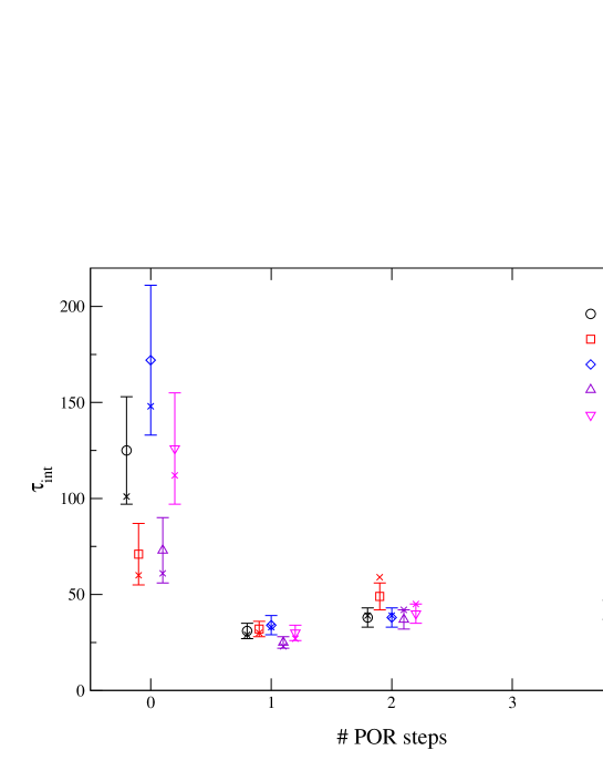
Figure 8.1: Integrated autocorrelation times of different operators using different update algorithms (1 Metropolis step + $n$ POR steps, $n=$ 0, 1, 2, 4) for the $\xi=2$ action. The autocorrelation times displayed by the open symbols as well as the errors have been determined by the method of Sokal, the crosses display the corresponding results obtained with the method of QCD-TARO.

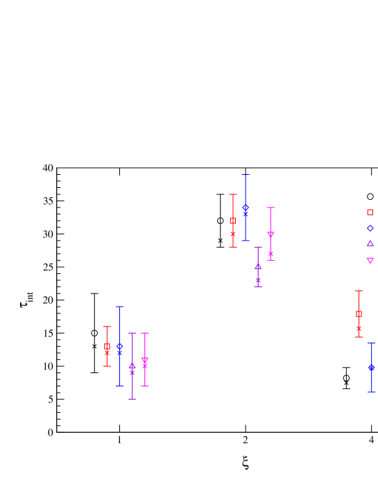
Figure 8.2: Integrated autocorrelation times of different operators using 1 Metropolis + 1 OR updates for the $\xi=1,2,4$ actions. The autocorrelation times displayed by the open symbols as well as the errors have been determined by the method of Sokal, the crosses display the corresponding results obtained with the method of QCD-TARO.

Table 8.3 lists the average change per link for Metropolis and POR updates using the perfect $\xi=2$ action at different values of the coupling $\beta$. It turns out that the average change of POR updates is about a factor of 10 larger than in the case of Metropolis updates; the normalised values are changing slowly with the lattice scale.

$\xi$	$\beta$	$\langle\Box\rangle$	$\frac{1}{\langle\Box\rangle}(\Delta U)_{\text{upd}}^{\text{Metropolis}}$	$\frac{1}{\langle\Box\rangle}(\Delta U)_{\text{upd}}^{\text{POR}}$
1	2.86	1.917	0.0652	0.472
	3.05	1.846	0.0527	0.486
	3.40	1.735	0.0660	0.506
2	3.00	1.885	0.0546	0.613
	3.15	1.702	0.0552	0.584
	3.30	1.584	0.0568	0.577
	3.50	1.487	0.0572	0.574
4	3.00	1.750	0.0400	0.328

Table 8.3: The average change per link for Metropolis and pseudo over-relaxation updates for the classically perfect actions with anisotropies $\xi=1,2,4$, normalised by the plaquette expectation value $\langle\Box\rangle=\langle N_{c}-\text{Re Tr }U^{\text{pl}}\rangle$.

Comparing configurations separated by $N$ MC updates using the measure eq. 8.11, we obtain the following (obvious) behaviour:

$$(\Delta U)_{\text{upd}}(N)=3-\alpha_{0}\cdot(1-q)^{N},$$ (8.12)

where $(\Delta U)_{\text{upd}}=3$ indicates that the configurations are completely independent on the level of gauge links. The factor $q$ determines the speed of the decorrelation. The results, obtained using only 20 starting configurations for each anisotropy and update and performing 100 sweeps each are displayed in Table 8.4. It turns out that these results are already completely stable. Obviously, these numbers disclose no secret and it is clear that all the effects apparent in the autocorrelation times, Tables 8.1, 8.2, stem from larger range correlations. Note as well, that the measure, eq. 8.11 is not gauge invariant, i.e. the gauge transform of a configuration may show to be completely independent, $(\Delta U)_{\text{upd}}=3$, of the initial configuration.

$\xi$	1 M	1 POR	1 M + 1 POR	1 M + 2 POR	1 M + 4 POR
	$q$	$q$	$q$	$q$	$q$
1	0.015	0.183	0.102	0.128	0.152
2	0.012	0.174	0.094	0.121	0.143
4	0.008	0.064	0.037	0.046	0.054

Table 8.4: The speed of the link decorrelation $q$ (see text) for different updates at different anisotropies.

8.5 The Computational Overhead

One very important quantity of an improved action is its computational overhead compared to the standard (i.e. Wilson) action.

To measure the effective gain or loss of an action is a very difficult task that depends very strongly on the application (spectroscopy, thermodynamics etc.), on the lattice sizes and lattice spacings used and as well on the architecture of the computers (scalar, vector, parallel and a lot of more subtle details) used.

Here, we will thus simply give raw ratios between the anisotropic perfect action, the widely used Symanzik and tadpole improved action and the Wilson action. It is clear that our parametrisation which is quite sophisticated has a large “raw” overhead, mainly due to the large number of operators that are affected if one link is changed in the MC update. Presently, our parametrisation is probably the most complex one that may still be considered to be utilised in numerical simulations of pure gauge theory. Although, in principle, the fit to the exact perfect action could be done much better, e.g. employing double smearing or including diagonal links into the smearing, such a procedure would surely make it unsuitable for MC simulations. Of course, if the gauge action is used together with (quenched or even dynamical) fermions, the computational cost of the gauge part is rather negligible, even better parametrisations of perfect actions might be imaginable in this case.

Table 8.5 compares the perfect anisotropic action to the Symanzik/tadpole-improved action of [42] and the Wilson action on lattices of size $8^{4}$ on an Alpha workstation. The numbers refer to the pure Metropolis update of each link of the configuration (“1 sweep”).

action	$t_{\text{sweep}}$ [s]	$t_{\text{act}}/t_{\text{Wilson}}$
Wilson	0.095	1
Symanzik	0.53	5.6
Perfect	6.3	66

Table 8.5: The updating time (1 sweep on a $8^{4}$ lattice) and the computational overhead of the perfect anisotropic action, compared to the Symanzik and tadpole improved action [42] and the standard Wilson action.

Chapter 9 Conclusions and Prospects

In this work, we have presented the construction and parametrisation of a classically perfect anisotropic SU(3) gauge action based on the Fixed Point Action technique. The recently parametrised isotropic FP action as well as its parametrisation ansatz using mixed polynomials of plaquettes built from single gauge links as well as from smeared links, have been the starting point. Performing one and two purely spatial blocking (RG) steps, respectively, starting from the isotropic action, and adapting the parametrisation to distinguish between spatial and temporal directions, we have obtained parametrised classically perfect actions with anisotropies $\xi=2$ and 4. That the method works has been checked as well in the context of scalar fields and in the quadratic approximation for SU(3) gauge theory. The $\xi=2$ action has been tested extensively in measurements of the torelon dispersion relation, of the static quark-antiquark potential, of the deconfining phase transition as well as of the low-lying glueball spectrum of pure gauge theory. For the $\xi=4$ action we have checked that the renormalisation of the anisotropy remains small and that it exhibits no pathologies in Monte Carlo simulations. For both actions (and additionally the isotropic FP action) autocorrelation times have been measured and the computational overhead, compared to the widely-used anisotropic tadpole and tree-level improved action as well as to the standard Wilson gauge action, has been determined.

The results of the torelon measurements show that the renormalisation of the anisotropy (due to quantum corrections and parametrisation artifacts) is small (below 10% for $\xi=2$ and 4). The rotational invariance of the action has been examined by measuring the static quark-antiquark potential, including separations corresponding to a large set of lattice vectors, again with good results. The glueball measurements, including some rather heavy states, confirm that the use of anisotropic lattices facilitates spectroscopy when heavy states are present. Compared to the isotropic simulations, with the same amount of computational work it is possible to resolve states with considerably larger energy, allowing reliable continuum extrapolations from larger ranges of the lattice spacing. The mass of the scalar glueball with quantum numbers $J^{PC}=0^{++}$ is measured to be considerably lighter (1440(40) MeV) compared to masses obtained by other groups (around 1670 MeV); furthermore it shows large cut-off effects when it is measured on a lattice with spatial lattice spacing $a_{s}\approx 0.25$ fm, which could be caused by a large sensitivity of the action to a critical point in the fundamental-adjoint coupling plane, due to adjoint terms in the action. However, the sources of possible errors in measurements of the glueball spectrum are manifold and there is no ultimate statement about the goodness of the parametrised classically perfect actions.

During our studies, we have noticed that the examination of scaling properties of lattice gauge actions is a very delicate problem: Quantities which can be reliably measured and which are not very sensitive to systematic factors (such as the volume, other states mixing with the observed ones, the method used for extracting the mass etc.), such as the critical temperature or the hadronic scale $r_{0}$ (for moderate lattice spacings) generally exhibit rather small cut-off effects and thus demand very large statistics, if the differences between the actions should be explicitly identified. On the other hand, some glueball states show large cut-off effects which make the glueball spectrum another interesting object to study scaling violations. As pointed out in this work, however, there are a lot of systematic factors making the extraction of the pure lattice artifacts difficult. The task of comparing different actions is even more difficult if the measurements and analyses are performed independently by different groups which introduces additional systematic discrepancies and ambiguities.

Let us therefore conclude that despite the rich parametrisation, the correspondence to the classically perfect FP action and the approximate scale invariance of classical instanton solutions there is no conclusive evidence of the parametrised classically perfect actions (isotropic as well as anisotropic) behaving significantly better than other improved actions (such as the tadpole and tree-level improved anisotropic gauge action) — however, there is also no evidence for the converse. What is clear and what one has to consider if one is about to plan a project where the update of the gauge configurations takes a considerable part of the computer time, is the considerable overhead of the parametrisation compared to other actions.

For the future, very accurate scaling tests comparing the classically perfect actions to other improved gauge actions are desirable. On one hand, these can include large statistics measurements of the critical temperature and the hadronic scale, on the other hand, one might perform very careful simulations determining the glueball spectrum, including all the limits to be taken and excluding all known sources of errors. These simulations should all be performed by the same collaboration in order to minimise systematic discrepancies coming from the analyses.

Another promising plan would be to gain control about the adjoint operators present in the parametrisation of the classically perfect actions in order to circumvent the critical point in the adjoint coupling plane such that the influence of the scalar dip is minimised.

Appendix A The FP Action for Scalar Field Theory

A simple way to get the lattice Fixed Point Action for $d=2$ free scalar theory is performing one single renormalisation group transformation (RGT) with an infinitely large scale factor starting in the continuum, a procedure called blocking out of continuum. The lattice is laid over the continuum field which is averaged over certain regions around the future lattice sites to obtain the lattice fields. The resulting FP action depends on the form of the averaging (corresponding to the blocking in finite scale RGTs) but the procedure presented here will be completely general.

We use the following RGT, accomplishing the task of averaging the continuum field $\varphi(x)$ to get to the lattice field $\phi_{n}$, where the form of the averaging is described by the function $\Pi(x)$

$$e^{-S^{FP}(\phi)}=\int\!\mathcal{D}\varphi(x)\,e^{-\frac{1}{2}\int\!d^{2}x\,\partial_{\mu}\varphi(x)\partial_{\mu}\varphi(x)-\kappa\sum\limits_{n}(\phi_{n}-\int\!d^{2}x\,\Pi(na-x)\varphi(x))^{2}},$$ (A.1)

the parameter $\kappa$ is again allowing the lattice field to fluctuate around the exact average of the continuum field (largely for small $\kappa$). The averaging is normalised to $\int d^{2}x\Pi(x)=1$. To account for an anisotropy, $a_{1}\neq a_{2}$, we perform the calculation using dimensionful quantities, the symbol $a$ is a shorthand notation for $(a_{1},a_{2})$.

Our goal is to obtain the FP propagator $D^{\text{FP}}$ on the lattice, we thus calculate the lattice two-point function $D(n-n^{\prime})=\langle\phi_{n}\phi_{n^{\prime}}\rangle$ in this theory:

$$D(n-n^{\prime})=\frac{1}{Z}\int\!\mathcal{D}\phi\,e^{-\frac{1}{2}\sum\limits_{n,r}\rho(r)\phi_{n}\phi_{n+r}}\phi_{n}\phi_{n^{\prime}};$$ (A.2)

inserting eq. A.1 we get

$$\frac{1}{Z}\int\!\mathcal{D}\phi\mathcal{D}\varphi\,e^{-\frac{1}{2}\int\!d^{2}x\,\partial_{\mu}\varphi(x)\partial_{\mu}\varphi(x)-\kappa\sum\limits_{n}(\phi_{n}-\int\!d^{2}x\,\Pi(na-x)\varphi(x))^{2}}\phi_{n}\phi_{n^{\prime}}.$$ (A.3)

The blocking (averaging) kernel is now Fourier transformed in the continuum:

$$K(n)=\int\!d^{2}x\,\Pi(na-x)\varphi(x):$$ (A.4)

$$\Pi(na-x)=\int\limits_{p}e^{ip(na-x)}\Pi(p),$$ (A.5)

$$\varphi(x)=\int\limits_{k}e^{ikx}\varphi(k),$$ (A.6)

thus

$$K(n)=\int d^{2}x\int\limits_{p}\int\limits_{k}e^{ipna}e^{i(k-p)x}\Pi(p)\varphi(k)=\int\limits_{k}e^{ikna}\Pi(k)\varphi(k).$$ (A.7)

Now we split up the continuum momentum variables $k_{\mu}$ according to:

$$k_{1}=q_{1}+\frac{2\pi}{a_{1}}l_{1},\quad k_{2}=q_{2}+\frac{2\pi}{a_{2}}l_{2}$$ (A.8)

with $q_{1}$, $q_{2}$ being lattice momenta in the respective Brillouin zones:

$$q_{1}\in\left(-\frac{\pi}{a_{1}},\frac{\pi}{a_{1}}\right),\quad q_{2}\in\left(-\frac{\pi}{a_{2}},\frac{\pi}{a_{2}}\right)$$ (A.9)

In the following, we will use the notation $k=q+\frac{2\pi}{a}l$ for convenience, where $k=(k_{1},k_{2})$. Inserting this replacement, we get:

$$\int\limits_{-\infty}^{\infty}\!\frac{d^{2}k}{(2\pi)^{2}}\,e^{ikna} = \sum\limits_{l=-\infty}^{\infty}\int\limits_{-\frac{\pi}{a_{1}}}^{\frac{\pi}{a_{1}}}\!\frac{dq_{1}}{2\pi}\,\int\limits_{-\frac{\pi}{a_{2}}}^{\frac{\pi}{a_{2}}}\!\frac{dq_{2}}{2\pi}\,e^{i(q_{1}+\frac{2\pi}{a_{1}}l_{1})n_{1}a_{1}}e^{i(q_{2}+\frac{2\pi}{a_{2}}l_{2})n_{2}a_{2}}$$ (A.10)

$$= \int\limits_{q}e^{iqna}\sum\limits_{l=-\infty}^{\infty},$$

using the shorthand notation

$$\int\limits_{q}=\int\limits_{-\frac{\pi}{a_{1}}}^{\frac{\pi}{a_{1}}}\!\frac{dq_{1}}{2\pi}\,\int\limits_{-\frac{\pi}{a_{2}}}^{\frac{\pi}{a_{2}}}\!\frac{dq_{2}}{2\pi}.$$ (A.11)

Using this, our two-point function reads:

$$\frac{1}{Z}\int\!\mathcal{D}\varphi\int\!\mathcal{D}\phi_{n}\,e^{-\frac{1}{2}\int\!d^{2}x\,\partial_{\mu}\varphi(x)\partial_{\mu}\varphi(x)-\kappa\sum\limits_{n}[\phi_{n}-\int\limits_{q}e^{iqna}\sum\limits_{l=-\infty}^{\infty}\Pi(q+\frac{2\pi}{a}l)\varphi(q+\frac{2\pi}{a}l)]^{2}}\phi_{n}\phi_{n^{\prime}}.$$ (A.12)

We replace $\phi_{n}$ by

$$\phi_{n}^{*}=\phi_{n}-\int\limits_{q}e^{iqna}\stackrel{{\scriptstyle b(q)}}{{\overbrace{\sum\limits_{l=-\infty}^{\infty}\Pi(q+\frac{2\pi}{a}l)\varphi(q+\frac{2\pi}{a}l)}}}$$ (A.13)

and get:

$$\frac{1}{Z}\int\!\mathcal{D}\varphi\int\!\mathcal{D}\phi_{n}^{*}\,(\phi_{n}^{*}+\int\limits_{q}e^{iqna}b(q))(\phi_{n^{\prime}}^{*}+\int\limits_{q}e^{iqn^{\prime}a}b(q))e^{-\frac{1}{2}\int\!d^{2}x\,\partial_{\mu}\varphi(x)\partial_{\mu}\varphi(x)-\kappa\sum\limits_{n}(\phi_{n}^{*})^{2}}.$$ (A.14)

Performing the integration over $\phi_{n}^{*}$, the terms linear in $\phi_{n}^{*}$ disappear.

If we integrate both sides of eq. A.1 with respect to $\phi_{n}$ we get $Z$ on the l.h.s. and $Z_{\varphi}Z_{\phi}$ on the r.h.s., with

$$Z_{\varphi}=\int\!\mathcal{D}\varphi\,e^{-\frac{1}{2}\int d^{2}x\partial_{\mu}\varphi(x)\partial_{\mu}\varphi(x)}$$ (A.15)

and

$$Z_{\phi}=\int\!\mathcal{D}\phi_{n}\,e^{-\kappa\sum\limits_{n}(\phi_{n}-\int\!d^{2}x\,\Pi(na-x)\varphi(x))^{2}}.$$ (A.16)

Using this notation we may write eq. A.14 as:

$$\frac{Z_{\varphi}}{Z}\int\!\mathcal{D}\phi_{n}^{*}\,\phi_{n}^{*}\phi_{n^{\prime}}^{*}e^{-\kappa\sum\limits_{n}(\phi_{n}^{*})^{2}}$$ (A.17)

$$+\frac{Z_{\phi}}{Z}\int\!\mathcal{D}\varphi\int\limits_{q}\!e^{iqna}b(q)\int\limits_{q}\!e^{iqn^{\prime}a}b(q)e^{-\frac{1}{2}\int\!d^{2}x\,\partial_{\mu}\varphi(x)\partial_{\mu}\varphi(x)}.$$ (A.18)

The first term is just

$$\frac{Z_{\varphi}}{Z}\cdot\frac{1}{\kappa}\delta_{n,n^{\prime}}\cdot Z_{\phi}=\frac{1}{\kappa}\delta_{n,n^{\prime}}=\frac{a_{1}a_{2}}{\kappa}\int\limits_{q}e^{iq(n-n^{\prime})a},$$ (A.19)

the second term reads

$$\frac{Z_{\phi}}{Z}\int\!\mathcal{D}\varphi\left[\int\limits_{q}e^{iq(n-n^{\prime})a}\sum\limits_{l=-\infty}^{\infty}\Pi(k)\varphi(k)\Pi^{{\dagger}}(k)\varphi^{{\dagger}}(k)\right]e^{-\frac{1}{2}\int\!d^{2}x\,\partial_{\mu}\varphi(x)\partial_{\mu}\varphi(x)},$$ (A.20)

after inserting the content of $b(q)$. Using eq. A.15, the definition of $Z_{\varphi}$, we get

$$\int\!\mathcal{D}\varphi\,\varphi(q+\frac{2\pi}{a}l)\varphi^{{\dagger}}(q+2\pi l)e^{-\frac{1}{2}\int\!d^{2}x\,\partial_{\mu}\varphi(x)\partial_{\mu}\varphi(x)}=Z_{\varphi}\cdot d(q+2\pi l),$$ (A.21)

and thus the second term is just

$$\int\limits_{q}e^{iq(n-n^{\prime})a}\sum\limits_{l=-\infty}^{\infty}\Pi(q+\frac{2\pi}{a}l)d(q+\frac{2\pi}{a}l)\Pi^{{\dagger}}(q+\frac{2\pi}{a}l);$$ (A.22)

together with the first term:

$$D(n-n^{\prime})=\int\limits_{q}e^{iq(n-n^{\prime})a}\left[\frac{1}{\kappa}+\sum\limits_{l=-\infty}^{\infty}\Pi(q+2\pi l)d(q+2\pi l)\Pi^{{\dagger}}(q+2\pi l)\right].$$ (A.23)

Thus we get $\rho(q)$:

$$\frac{1}{\rho(q)}=\sum\limits_{l=-\infty}^{\infty}\left[\Pi(q+\frac{2\pi}{a}l)d(q+\frac{2\pi}{a}l)\Pi^{{\dagger}}(q+\frac{2\pi}{a}l)\right]+\frac{a_{1}a_{2}}{\kappa}.$$ (A.24)

Setting $a_{1}=a_{2}=1$ we get back the isotropic FP action as expected.

We are interested in couplings $\rho(q)$ on the lattice which are dimensionless quantities. In order to achieve this, we rescale the above formula by dividing it by $a_{1}a_{2}$, this absorbs the product in the $\kappa$-term, also, the propagator $d(k)$ will become dimensionless:

$$d(k)=\frac{1}{a_{1}a_{2}}\frac{1}{(q_{1}+\frac{2\pi}{a_{1}}l_{1})^{2}+(q_{2}+\frac{2\pi}{a_{2}}l_{2})^{2}}=\frac{1}{\xi^{-1}(p_{1}+2\pi l_{1})^{2}+\xi(p_{2}+2\pi l_{2})^{2}},$$ (A.25)

where $p_{1}$, $p_{2}$ are dimensionless momenta, $p_{\mu}\in(-\pi,\pi)$, and $\xi=\frac{a_{1}}{a_{2}}$ is the anisotropy parameter as defined above.

Appendix B The Quadratic Approximation for Gauge Fields

In this Appendix we describe the calculation of the couplings $\rho_{\mu\nu}(r)$ in the quadratic approximation to the classically perfect action, eq. 5.16,

$$S^{\text{FP}}=\frac{1}{2N_{c}}\sum_{n,r}\rho_{\mu\nu}(r)\text{Tr}[A_{\mu}(n+r)A_{\nu}(n)]+\text{O}(A^{3}).$$ (B.1)

B.1 The Anisotropic Recursion Relation

At the quadratic level, the recursion relation corresponding to eqs. 1.5, 4.1, 4.2 reads in standard matrix notation

$$\frac{1}{\xi V_{B}}\sum_{k_{B}}\text{Tr}\left\{B^{\dagger}(k_{B})\Xi\rho^{\prime}(k_{B})\Xi B(k_{B})\right\}$$ (B.2)

$$= \text{min}_{\{A\}}\left(\frac{1}{\xi V}\sum_{k}\text{Tr}\left\{A^{\dagger}(k)\Xi\rho(k)\Xi A(k)\right\}\right.$$

$$\left.\hskip 14.22636pt+\frac{1}{\xi V_{B}}\sum_{k_{B}}\text{Tr}\left\{(\Gamma(k_{B})-B(k_{B}))^{\dagger}\Xi\kappa\Xi(\Gamma(k_{B})-B(k_{B}))\right\}\right),$$

where $V_{B}=\frac{1}{16}V$ is the volume of the blocked lattice, $B(k_{B})$ denotes the blocked gauge configuration, $A_{\mu}$, $B_{\mu}$ are the gauge potentials of the configurations $U$, $V$,

$$V_{\mu}(n_{B})=e^{iB_{\mu}(n_{B})},\quad U_{\mu}(n)=e^{iA_{\mu}(n)}$$ (B.3)

and

$$\Xi=\left(\begin{array}[]{cccc}1&&&\\ &1&&\\ &&1&\\ &&&\xi\end{array}\right).$$ (B.4)

In the above formula $\rho,\kappa$ are expressed in units of $a_{s}$ and the blocking function $\omega(k)$ is a dimensionless quantity, while

$$k_{\mu}=k_{\mu}^{\text{df}}a_{\mu}\quad\text{and}\quad X_{\mu}=\frac{\prod_{\nu=0}^{3}a_{\nu}}{a_{\mu}}X^{\text{df}}_{\mu},$$ (B.5)

where $X_{\mu}$ is a common symbol for the gauge potentials $A_{\mu}$, $B_{\mu}$ etc.

B.2 The Calculation of the Couplings

The blocking used in this work (see Section 4.2) corresponds to

$$\Xi\cdot\Gamma(k_{B})=\frac{1}{16}\sum_{l=0}^{1}\omega(\frac{k_{B}}{2}+\pi l)\Xi A(\frac{k_{B}}{2}+\pi l),\quad l=(l_{1},l_{2},l_{3},l_{4}),$$ (B.6)

with

$$\omega_{\mu\nu}=(1+e^{ik_{\mu}})\left[c_{0}\delta_{\mu\nu}+6c_{1}\tau_{\mu\nu}^{(1)}(k)+12c_{2}\tau_{\mu\nu}^{(2)}(k)+8c_{3}\tau_{\mu\nu}^{(3)}(k)\right].$$ (B.7)

The tensor $\omega_{\mu\nu}$ is fixed by the form of the blocking kernel, where up to this order the linear contributions $\tau_{\mu\nu}^{(i)}$ to the fuzzy link operator have to be taken into account. They can be written as

$$\tau^{(1)}_{\mu\nu}(k) \!\!\!=\!\!\! \frac{1}{6}\left[\;\widehat{k}_{\mu}\widehat{k}_{\nu}^{*}+\delta_{\mu\nu}(6-\gamma)\;\right],$$

$$\tau^{(2)}_{\mu\nu}(k) \!\!\!=\!\!\! \frac{1}{24}\left[\;\widehat{k}_{\mu}\widehat{k}_{\nu}^{*}(8-\gamma+\widehat{k}_{\mu}\widehat{k}_{\mu}^{*}+\widehat{k}_{\nu}\widehat{k}_{\nu}^{*})+\delta_{\mu\nu}(24-8\gamma+\gamma^{2}-\eta-\gamma\widehat{k}_{\mu}\widehat{k}_{\mu}^{*})\;\right],$$

$$\tau^{(3)}_{\mu\nu}(k) \!\!\!=\!\!\! \frac{1}{48}\Big{[}\;\widehat{k}_{\mu}\widehat{k}_{\nu}^{*}(24-6\gamma+\gamma^{2}-\eta+6\widehat{k}_{\mu}\widehat{k}_{\mu}^{*}-2\gamma\widehat{k}_{\mu}\widehat{k}_{\mu}^{*}+2(\widehat{k}_{\mu}\widehat{k}_{\mu}^{*})^{2}+6\widehat{k}_{\nu}\widehat{k}_{\nu}^{*}$$ (B.8)

$$~{}~{}~{}~{}~{}~{}~{}~{}~{}~{}~{}~{}~{}-2\gamma\widehat{k}_{\nu}\widehat{k}_{\nu}^{*}+2(\widehat{k}_{\nu}\widehat{k}_{\nu}^{*})^{2}+2\widehat{k}_{\mu}\widehat{k}_{\mu}^{*}\widehat{k}_{\nu}\widehat{k}_{\nu}^{*})$$

$$~{}~{}~{}~{}+\delta_{\mu\nu}(48-24\gamma+6\gamma^{2}-\gamma^{3}-6\gamma\widehat{k}_{\mu}\widehat{k}_{\mu}^{*}+2\gamma^{2}\widehat{k}_{\mu}\widehat{k}_{\mu}^{*}-2\gamma(\widehat{k}_{\mu}\widehat{k}_{\mu}^{*})^{2}$$

$$~{}~{}~{}~{}~{}~{}~{}~{}~{}~{}~{}~{}~{}~{}+3\gamma\eta-2\epsilon-6\eta-2\eta\widehat{k}_{\mu}\widehat{k}_{\mu}^{*})\Big{]}.$$

The lattice momentum $\widehat{k}_{\mu}$ is defined by

$$\widehat{k}_{\mu}=e^{ik_{\mu}}-1$$ (B.9)

and the following definitions have been made for convenience:

$$\gamma\doteq|\hat{k}|^{2}\doteq\sum_{\mu}\widehat{k}_{\mu}\widehat{k}_{\mu}^{*},\quad\eta\doteq\sum_{\mu}(\widehat{k}_{\mu}\widehat{k}_{\mu}^{*})^{2},\quad\epsilon\doteq\sum_{\mu}(\widehat{k}_{\mu}\widehat{k}_{\mu}^{*})^{3}.$$

The four parameters of the RGT in eq. B.7 have been optimised in [60] and have the values:

$$c_{1}=0.07,\quad c_{2}=0.016,\quad c_{3}=0.008,\quad\kappa=8.8.$$ (B.10)

From eq. B.2, using the relation eq. B.6, we obtain a recursion relation for the inverse of the couplings $D_{\mu\nu}(k)=\rho^{-1}_{\mu\nu}(k)$:

$$D^{\prime}_{\mu\nu}(k_{B})=\frac{1}{16}\sum_{l=0}^{1}\left[\Xi\omega(\frac{k_{B}}{2}+\pi l)D(\frac{k_{B}}{2}+\pi l)\omega^{\dagger}(\frac{k_{B}}{2}+\pi l)\Xi\right]_{\mu\nu}+\Xi\frac{1}{\kappa}\Xi.$$ (B.11)

One way to find the FP solution for the propagator is to start from the anisotropic Wilson propagator and to iterate the propagator to the FP. As we have to invert the coupling tensors $\rho_{\mu\nu}$ and $\rho^{\prime}_{\mu\nu}$ we have to introduce a temporary gauge fixing. The gauge–fixed anisotropic Wilson action reads

$$D^{(0)}_{\mu\nu}(k)=\frac{\delta_{\mu\nu}}{\sum_{i}|\widehat{k}_{i}|^{2}+\xi^{2}|\widehat{k}_{4}|^{2}}+\alpha\frac{\widehat{k}_{\mu}\widehat{k}_{\nu}^{*}}{(\sum_{i}|\widehat{k}_{i}|^{2}+\xi^{2}|\widehat{k}_{4}|^{2})^{2}}$$ (B.12)

At the end the gauge–fixing will be removed, which corresponds to the limit $\alpha\rightarrow\infty$.

Using the gauge relation

$$\omega_{\mu\nu}(k)\widehat{k}_{\nu}=\widehat{2k_{\mu}}$$ (B.13)

one can show that starting from the standard propagator, after an arbitrary number of iterations, the propagator $D_{\mu\nu}(k)$ assumes the form

$$D_{\mu\nu}(k)=G_{\mu\nu}(k)+\alpha f(k)\widehat{k}_{\mu}\widehat{k}_{\nu}^{*}$$ (B.14)

with $G_{\mu\nu}(k)$ and $f(k)$ independent of $\alpha$. It may now be shown [60] that in the limit $\alpha\rightarrow\infty$ the function $f(k)$ (which is the only part differing from the isotropic case) drops out and the result for the couplings is

$$\rho_{\mu\nu}(k)=G^{-1}_{\mu\nu}(k)-\frac{G^{-1}_{\mu\rho}(k)\widehat{k}_{\rho}\cdot\widehat{k}_{\sigma}^{*}G^{-1}_{\sigma\nu}(k)}{\widehat{k}_{\sigma}^{*}G^{-1}_{\sigma\rho}(k)\widehat{k}_{\rho}}.$$ (B.15)

To construct the anisotropic propagator $\rho^{-1}(q)$ numerically we perform 3 recursions on a $32^{4}$ lattice using the $\kappa$ value obtained optimising the locality in the isotropic case, $\kappa=8.8$. We study the dependence of the number of recursions and do not discover any notable changes if we change it from 3 to 4 – the FP quadratic propagator is thus reached already after 3 recursions. The following steps, inverting $\rho^{-1}(q)$ to get the couplings in momentum space, removing the gauge fixing (analytically) and the subsequent Fourier transformation do not change from the isotropic case described in [59, 60].

A priori there is no reason why the parameter $\kappa$ occurring in the recursion relation should be chosen to have the same value for the spatial and the temporal part of the relation, i.e. one may think about changing $\kappa$ to the more general form

$$\kappa\longrightarrow\tilde{\kappa}=\left(\begin{array}[]{cccc}\kappa_{s}&&&\\ &\kappa_{s}&&\\ &&\kappa_{s}&\\ &&&\kappa_{t}\end{array}\right).$$

There are two “natural” choices, either stick to the $\delta_{\mu\nu}$ form of $\kappa$ and set $\kappa_{t}=\kappa_{s}=8.8$ or change it to $\kappa_{t}=\xi^{2}\kappa_{s}=\xi^{2}\cdot 8.8$ to compensate for the insertion of the two $\Xi$-matrices in eq. B.11. Performing numerical studies (in the full theory) it indeed turns out that the latter choice is the one yielding actions that are well parametrisable.

Appendix C The Norm of the Anisotropic APE Action

In this Appendix we derive the anisotropic normalisation condition which makes sure that the action goes over to the continuum form for very smooth fields.

We first define for a general continuum gauge field a dimension 4 operator $R_{0}$:

$$R_{0}=-\frac{1}{2}\sum_{\mu\nu}\text{Tr}(\mathcal{F}_{\mu\nu}^{2}).$$ (C.1)

To work out the form of the conditions for our parametrisation of the action we use constant gauge non–Abelian gauge potentials, $\partial_{\mu}A_{\nu}=0$. In the continuum we have

$$\mathcal{F}_{\mu\nu}=[A_{\mu},A_{\nu}].$$ (C.2)

The constant non–Abelian gauge–field is defined on the lattice as

$$\mathcal{A}_{\mu}=i\alpha_{\mu}\cdot\frac{1}{2}\sigma_{\mu},$$ (C.3)

where $\sigma_{k}$, $k$=1, 2, 3 are the Pauli matrices and $\sigma_{4}=(\sigma_{1}+\sigma_{2}+\sigma_{3})/\sqrt{3}$.

To obtain the normalisation condition we expand our anisotropic gauge action, parametrised as described in Section 4.3, in powers of $\alpha_{\mu}$ keeping the spatial indices $k=1,2,3$ and the temporal index 4 separate. This yields two operators $R_{0}^{\text{s}}\sim O(a_{s}^{4})$ and $R_{0}^{\text{t}}\sim O(a_{s}^{2}a_{t}^{2})$. Up to quartic order in $a_{s}$, $a_{t}$ the action can be expressed in $R_{0}^{\text{s}}$ and $R_{0}^{\text{t}}$:

$$\mathcal{A} = \frac{R_{0}^{\text{t}}\xi}{2}\left[2c_{12}p_{01}^{\text{tm}}+p_{10}^{\text{sp}}+p_{01}^{\text{sp}}\left(1+2c_{11}+2\eta_{1}c_{11}\right)\right]$$ (C.4)

$$+\frac{R_{0}^{\text{s}}}{2\xi}\left[2\eta_{3}c_{11}p_{01}^{\text{sp}}+p_{10}^{\text{tm}}+p_{01}^{\text{tm}}\left(1+2c_{13}+\eta_{2}c_{13}+\eta_{4}c_{12}\right)\right],$$

where all parameters $\eta$, $c$ denote the constant ($0^{\text{th}}$ order) terms in the polynomials in $x_{\mu}$; the higher orders do not contribute due to $x_{\mu}\rightarrow 0$ for very smooth fields.

The coefficient of $R_{0}$ in eq. C.1 is required to be 1 and thus a simple comparison yields the two normalisation conditions for our parametrisation of the anisotropic gauge action:

$$p^{\text{s}p}_{01}+p^{\text{s}p}_{10}+2p^{\text{s}p}_{01}c_{11}+2p^{\text{t}m}_{01}c_{12}+2p^{\text{s}p}_{01}c_{11}\eta_{1} = \frac{1}{\xi},$$ (C.5)

$$p^{\text{t}m}_{01}+p^{\text{t}m}_{10}+2p^{\text{t}m}_{01}c_{13}+p^{\text{t}m}_{01}c_{13}\eta_{2}+2p^{\text{s}p}_{01}c_{11}\eta_{3}+p^{\text{t}m}_{01}c_{12}\eta_{4} = \xi.$$ (C.6)

These two conditions ensure that the parametrised action goes over to the continuum form with correct anisotropy if the action is applied on smooth fields. They are required to be fulfilled exactly for all our parameter sets.

Appendix D Action parameters

In this Appendix we collect the parameters of the FP and classically perfect actions that have been used or constructed throughout this work. The isotropic FP action presented in Section D.1 is the one that has been parametrised and examined closely in [1, 2, 3], results of these studies are collected briefly in Chapter 3. The isotropic action $\mathcal{A}_{5}^{444}$ in Section D.2 is an intermediate parametrisation valid on configurations typical for MC simulations that are minimised once, parametrised during the cascade process for the isotropic action. It is used in the spatial blocking (see Section 6.1) to minimise the coarse $\xi=2$ configurations, constructed using the ad-hoc anisotropic action presented in Section D.3. The resulting $\xi=2$ perfect action for coarse configurations is presented in Section D.4.

To repeat the blocking step, we need a $\xi=2$ action which is valid for $\xi=4$ configurations minimised once in a purely spatial blocking step. Such an intermediate action has been constructed, see Section D.5. The resulting $\xi=4$ action is presented in Section D.6.

D.1 The Isotropic FP Action

The parametrisation of the isotropic FP action is described in [1, 2, 3] as well as in Chapter 3. It describes the FP action well in the range of lattice spacings $0.03\text{ fm}\lesssim a\lesssim 0.3\text{ fm}$.

The set of parameters consists of four non-linear parameters $\eta^{(0)}$, $c_{1}^{(0)}$, $c_{2}^{(0)}$, $c_{3}^{(0)}$ describing the asymmetrically smeared links $W_{\mu}^{(\nu)}$ and fourteen linear parameters $p_{kl}$ with $0<k+l\leq 4$. This set approximates reasonably well the true FP action in the range of $a$ given above. (For smaller fluctuations — occurring e.g. in the intermediate steps of the parametrisation — we use polynomials for $\eta(x)$ and $c_{i}(x)$ up to forth order.)

The optimal non-linear parameters are found to be

$$\eta^{(0)}=-0.038445\,,\quad c_{1}^{(0)}=0.290643\,,\quad c_{2}^{(0)}=-0.201505\,,\quad c_{3}^{(0)}=0.084679\,.$$

The linear parameters are collected in Table D.1.

$p_{kl}$	$l=0$	$l=1$	$l=2$	$l=3$	$l=4$
$k=0$		0.442827	0.628828	-0.677790	0.176159
$k=1$	0.051944	-0.918625	1.064711	-0.275300
$k=2$	0.864881	-0.614357	0.165320
$k=3$	-0.094366	-0.020693
$k=4$	0.022283

Table D.1: The linear parameters $p_{kl}$ of the parametrised isotropic FP action.

D.2 The Intermediate Isotropic Action $\mathbf{\mathcal{A}_{5}^{444}}$

The intermediate isotropic action has been parametrised during the construction of the isotropic FP action. It is supposed to be valid on configurations that are obtained by minimising configurations typical for MC simulations once. It fulfills the $O(a^{2})$ Symanzik conditions (see [1, 2]) and uses fluctuation polynomials $x_{\mu}(n)$ (see Section 4.3.1), it thus smoothly approaches the continuum (high $\beta$) limit and is expected to interpolate between the rather coarse configurations mentioned above and the smooth limit. It is not intended to be used in MC simulations, its linear behaviour (see Section 1.4.5) is not checked, in addition the set of parameters is not as compact as might be possible.

This action has been used for the (spatial) minimisation of coarse $\xi=2$ configurations to describe the isotropic configurations on the r.h.s. of eq. 1.5.

The non-linear parameters describing order 3 polynomials are

$\eta^{(0)}=0.082$,	$\eta^{(1)}=0.292353$,	$\eta^{(2)}=0.115237$,	$\eta^{(3)}=0.011456$,
$c_{1}^{(0)}=0.282$,	$c_{1}^{(1)}=-0.302295$,	$c_{1}^{(2)}=-0.302079$,	$c_{1}^{(3)}=-0.052309$,
$c_{2}^{(0)}=0.054$,	$c_{2}^{(1)}=0.298882$,	$c_{2}^{(2)}=-0.081365$,	$c_{2}^{(3)}=-0.023762$,
$c_{3}^{(0)}=-0.201671$,	$c_{3}^{(1)}=0.022406$,	$c_{3}^{(2)}=0.004090$,	$c_{3}^{(3)}=0.014886$,
$c_{4}^{(0)}=-0.008977$,	$c_{4}^{(1)}=0.245363$,	$c_{4}^{(2)}=0.140016$,	$c_{4}^{(3)}=0.028783$.

The linear parameters are collected in Table D.2.

$p_{kl}$	$l=0$	$l=1$	$l=2$	$l=3$	$l=4$
$k=0$		0.629227	-0.556304	0.186662	-0.010110
$k=1$	-0.368095	0.852428	-0.199034	0.031614
$k=2$	0.389292	-0.207378	-0.010898
$k=3$	-0.054912	0.039059
$k=4$	-0.000424

Table D.2: The linear parameters $p_{kl}$ of the parametrised intermediate isotropic FP action $\mathcal{A}_{5}^{444}$.

D.3 “Ad-hoc” Anisotropic Actions

In the spatial blocking procedure described in Chapter 4 one needs coarse anisotropic ($\xi=$ 2, 4, 6, $\ldots$) gauge configurations which are spatially minimised leading to $\xi^{\prime}=\xi/2$ configurations. As the goal of this step is to obtain a perfect anisotropic action with anisotropy $\xi$ these coarse anisotropic configurations have to be produced using some other action that is already present. This requirement might seem to endanger the whole ansatz, however it is not crucial how the coarse configurations exactly look like as the perfectness of the resulting coarse action comes from the perfect action on the fine configuration as well as from the exactness of the RG transformation (see Section 1.3). Still, we try to create coarse configurations that might look similar to future ensembles produced using the perfect anisotropic action on the coarse level and whose minimised configurations appear to have an anisotropy approximately $\xi^{\prime}=\xi/2$ (i.e. which are isotropic in the case of the construction of the $\xi=2$ action).

In order to achieve this, we modify the isotropic FP action adding a term $(\xi^{2}-1)p_{10}^{st}$ (where $p_{10}^{st}$ denotes the simple temporal plaquette). This modification turns the isotropic Wilson action into the Wilson action with bare anisotropy $\xi$ and is expected to work approximately also for our FP action. The main argument of using this coarse action and not e.g. the anisotropic Wilson action is that due to the spatial lattice spacing $a_{s}$ being larger than the temporal spacing $a_{t}$, the $O(a_{s}^{2})$ artifacts are also expected to be larger than the $O(a_{t}^{2})$ effects. The modification described above should preserve the FP properties corresponding to $a_{s}$ and is thus expected to be considerably better than the naive anisotropic Wilson action.

Using this ad-hoc modification of the isotropic FP action (“ad-hoc” action) in MC simulations shows (as expected) that (at least for small anisotropies $\xi\lesssim 5$) its properties are not comparable with the ones of the isotropic FP action, however the generated ensembles resemble to the ones generated with true perfect anisotropic actions much more than ensembles generated by the Wilson action.

The anisotropies $\xi_{\text{ad-hoc}}$ that have to be used to generate coarse anisotropic configurations turning into minimised configurations with anisotropy $\xi^{\prime}$ are $\xi_{\text{ad-hoc}}\approx 3.2$ for $\xi^{\prime}=1$ and $\xi_{\text{ad-hoc}}\approx 6$ for $\xi^{\prime}=2$. However, this value of $\xi_{\text{ad-hoc}}$ varies considerably if $\beta$ is varied — but as stated at the beginning of this section, the exact form of the coarse configurations is not essential.

D.4 The $\mathbf{\xi=2}$ Perfect Action

The $\xi=2$ perfect action uses the parametrisation described in Sections 4.3.1, 4.3.2. The number of non-zero asymmetry values $\eta_{i}^{(0)}$ is 4, the parameters $c_{i}^{(0)}$ ($i=1,\ldots,3$) are splitted into 3 parameters depending on the contribution to the smeared plaquette. The linear parameters $p_{kl}$ are non-zero for $0<k+l\leq 4$ for spatial plaquettes and $0<k+l\leq 3$ for temporal plaquettes.

The non-linear parameters (constants in $x_{\mu}$) have the values

$\eta_{1}=-0.866007$,	$\eta_{2}=-0.884110$,	$\eta_{3}=2.212499$,	$\eta_{4}=1.141177$;
$c_{11}=0.399669$,	$c_{12}=0.519037$,	$c_{13}=-0.071334$,
$c_{21}=-0.076357$,	$c_{22}=-0.031051$,	$c_{23}=-0.282800$,
$c_{31}=0.032396$,	$c_{32}=-0.015844$,	$c_{33}=-0.046302$.

The linear parameters are collected in Table D.3

$p_{kl}^{ss}$	$l=0$	$l=1$	$l=2$	$l=3$	$l=4$
$k=0$		0.433417	0.098921	-0.116251	0.023295
$k=1$	0.217599	-0.272668	0.248188	-0.045278
$k=2$	0.316145	-0.180982	0.028817
$k=3$	-0.039521	0.003858
$k=4$	0.005443

$p_{kl}^{st}$	$l=0$	$l=1$	$l=2$	$l=3$
$k=0$		-0.190195	0.554426	-0.121766
$k=1$	1.521212	-0.328305	0.086655
$k=2$	0.011178	0.020932
$k=3$	0.022856

Table D.3: The linear parameters of the $\xi=2$ parametrised classically perfect action.

D.5 The $\mathbf{\xi=2}$ Intermediate Action

In order to be able to repeat the spatial blocking step constructing a $\xi\approx 4$ action based on the $\xi=2$ perfect action we need a parametrisation of the $\xi=2$ action which is valid on ($\xi\approx 2$) configurations that are obtained by spatially minimising coarse $\xi=4$ configurations once. To construct such an action, we perform a non-linear fit to the derivatives of 5 sets of two configurations each at $\beta=$ 6, 10, 20, 50, 100. The non-linear parameters are chosen to be linear in the fluctuation parameter $x_{\mu}(n)$. Having four different parameters $\eta$ and splitting up $c_{i}$ into three parameters (as it is done for all anisotropic parametrisations), this makes 20 non-linear parameters to be fitted which is quite at the edge of what is still possible on our computers (see Section 1.4.4), that is why we restrict the total number of configurations to 10. Rough checks performed on a larger number of configurations, with an even larger number of parameters show however, that the resulting non-linear parameters are stable and describe the data accurately.

The derivatives and action values of 5 sets of 10 configurations each are included in the linear fit (where the relative weight of the action values is chosen to be $1.9\cdot 10^{-2}$ for the configurations at $\beta=$ 50, 100 and $7.6\cdot 10^{-4}$ at $\beta=$ 6, 10, 20). A linear set where the parameters $p_{kl}$ are non-zero for $0<k+l\leq 3$ for spatial plaquettes and $0<k+l\leq 4$ for temporal plaquettes describes the full action very well concerning this data. Again, this parametrisation is not intended to be used in MC simulations, thus the linear behaviour of the action is not checked.

The non-linear parameters (linear in $x_{\mu}$) have the values

$\eta_{1}^{(0)}=-1.861267$,	$\eta_{1}^{(1)}=-0.327466$,	$\eta_{2}^{(0)}=-1.075610$,	$\eta_{2}^{(1)}=-0.550398$,
$\eta_{3}^{(0)}=2.750293$,	$\eta_{3}^{(1)}=0.089874$,	$\eta_{4}^{(0)}=1.107017$,	$\eta_{4}^{(1)}=0.265817$;
$c_{11}^{(0)}=0.520960$,	$c_{11}^{(1)}=0.006339$,	$c_{21}^{(0)}=-0.075219$,	$c_{21}^{(1)}=0.059506$
$c_{12}^{(0)}=0.266240$,	$c_{12}^{(1)}=0.121035$,	$c_{22}^{(0)}=-0.080771$,	$c_{22}^{(1)}=-0.021515$
$c_{13}^{(0)}=0.159372$,	$c_{13}^{(1)}=0.039564$,	$c_{23}^{(0)}=-0.043901$,	$c_{23}^{(1)}=0.009672$

The linear parameters are collected in Table D.4

$p_{kl}^{ss}$	$l=0$	$l=1$	$l=2$	$l=3$
$k=0$		0.088016	0.002225	-0.000285
$k=1$	0.341850	-0.015888	-0.004087
$k=2$	-0.053007	0.010121
$k=3$	0.010500

$p_{kl}^{st}$	$l=0$	$l=1$	$l=2$	$l=3$	$l=4$
$k=0$		0.280043	5.077727	-13.714872	12.739964
$k=1$	1.343946	-6.934825	27.673937	-32.288928
$k=2$	2.069084	-17.392027	28.248910
$k=3$	3.691733	-9.584760
$k=4$	0.712244

Table D.4: The linear parameters of the intermediate $\xi=2$ parametrised classically perfect action.

D.6 The $\mathbf{\xi=4}$ Perfect Action

The $\xi=4$ perfect action uses the parametrisation described in Sections 4.3.1, 4.3.2. The number of non-zero asymmetry values $\eta_{i}^{(0)}$ is 4, the parameters $c_{i}^{(0)}$ ($i=1,\ldots,3$) are splitted into 3 parameters depending on the contribution to the smeared plaquette. The linear parameters $p_{kl}$ are non-zero for $0<k+l\leq 3$ for spatial plaquettes and $0<k+l\leq 2$ for temporal plaquettes.

The non-linear parameters (constants in $x_{\mu}$) have the values

$\eta_{1}=-1.491457$,	$\eta_{2}=-1.115141$,	$\eta_{3}=1.510985$,	$\eta_{4}=7.721347$;
$c_{11}=2.014408$,	$c_{12}=0.128768$,	$c_{13}=0.162296$,
$c_{21}=-0.915620$,	$c_{22}=0.134445$,	$c_{23}=-0.013383$,
$c_{31}=1.166289$,	$c_{32}=0.061278$,	$c_{33}=0.000759$,

The linear parameters are collected in Table D.5

$p_{kl}^{ss}$	$l=0$	$l=1$	$l=2$	$l=3$
$k=0$		0.027625	0.000052	0.000000
$k=1$	0.072131	-0.016852	-0.000054
$k=2$	0.036818	0.003558
$k=3$	-0.007413

$p_{kl}^{st}$	$l=0$	$l=1$	$l=2$
$k=0$		0.795779	0.621286
$k=1$	2.130563	-0.286602
$k=2$	0.076086

Table D.5: The linear parameters of the $\xi=4$ parametrised classically perfect action.

Appendix E Variational Techniques

Normally, in a Monte Carlo simulation there are several operators that have an overlap with a state one would like to measure. In the case of glueballs, e.g., we have multiple shapes with combinations of different orientations having the same quantum numbers. Another method yielding several gauge operators with the same quantum numbers, is smearing (see Section 2.1.2). A priori it is unknown which operators have the largest contribution to a given state, it is therefore vital to have a method which takes into account the different operators according to their overlap with the desired state. In this Appendix we describe the variational techniques accomplishing this, used for all mass / energy determinations (torelons, static $q\bar{q}$-potential, glueballs).

E.1 Obtaining Mass Estimates

In a Monte Carlo simulation we measure the $N\times N$ correlation matrix of operators ${\cal O}_{\alpha}$

$$C_{\alpha\beta}(t)=\langle 0|{\cal O}_{\alpha}(t){\cal O}^{\dagger}_{\beta}(0)|0\rangle\,,$$ (E.1)

where $N$ is the number of operators having the same quantum numbers as the examined state. To determine the coefficients $v_{\alpha}$ of the linear combination $\sum_{\alpha=1}^{N}v_{\alpha}{\cal O}_{\alpha}$ which has the largest overlap to the ground state relative to the excited states one has to minimise the effective mass given by

$$m(t_{0},t_{1})=-\ln\left[\frac{(v,C(t_{1})v)}{(v,C(t_{0})v)}\right]/(t_{1}-t_{0}).$$ (E.2)

The vector $v$ is obtained by solving the generalised eigenvalue equation [153, 154]

$$C(t_{1})v=\lambda(t_{0},t_{1})C(t_{0})v\,,$$ (E.3)

where $0\leq t_{0}<t_{1}$.

Assume first that only the lowest lying $N$ states contribute to $C(t)$, i.e.,

$$C_{\alpha\beta}(t)=\sum_{n=1}^{N}\text{e}^{-E_{n}t}\psi_{n\alpha}\psi_{n\beta}^{*}\,,$$ (E.4)

where $E_{1}\leq E_{2}\leq\ldots\leq E_{N}$ are the energy levels in the given symmetry channel and $\psi_{n\alpha}=\langle 0|O_{\alpha}|n\rangle$ is the “wave function” of the corresponding state. The solution of eq. E.3 is given by the set of vectors $\{v_{n}\}$ dual to the wave functions, i.e., $(v_{n},\psi_{m})=\delta_{nm}$. Multiplying eq. E.4 by $v_{n}$ one obtains

$$C(t)v_{n}=\text{e}^{-E_{n}t}\psi_{n}=\text{e}^{-E_{n}(t-t_{0})}\text{e}^{-E_{n}t_{0}}\psi_{n}=\text{e}^{-E_{n}(t-t_{0})}C(t_{0})v_{n}\,.$$ (E.5)

This gives $\lambda_{n}(t_{0},t_{1})=\exp(-E_{n}(t_{1}-t_{0}))$ for the eigenvalues in eq. E.3. Of course, contributions from states with $n>N$ and statistical fluctuations distort eq. E.4, therefore the stability of eq. E.3 is an important issue.

Observe that eq. E.3 is well defined only for positive definite $C(t_{0})$. Because of statistical fluctuations, however, the measured correlation matrix $C(t_{0})$ is not necessarily positive for $t_{0}>0$. This is the reason why one usually considers only the $t_{0}=0$ case in applying the variational method, especially with a large number of operators. On the other hand, it is obvious that $C(0)$ is contaminated by highly excited states and contains only restricted information on the low lying part of the spectrum. Therefore it is desirable to take $t_{0}>0$. This can be achieved in the following way [155].

We first diagonalise $C(t_{0})$,

$$C(t_{0})\varphi_{i}=\lambda_{i}\varphi_{i},\quad\lambda_{1}\geq\ldots\geq\lambda_{N},$$ (E.6)

and project the correlation matrices to the space of eigenvectors corresponding to the $M$ highest eigenvalues,

$$C^{M}_{ij}(t)=(\varphi_{i},C(t)\varphi_{j}),\quad i,j=1,\ldots,M.$$ (E.7)

By choosing the operator space too large we introduce numerical instabilities caused by very small (even negative) eigenvalues with large statistical errors due to the fact that the chosen operator basis is not sufficiently independent on the given MC sample. By choosing $M$ appropriately we can get rid of those unstable modes while still keeping all the physical information. In this way we render the generalised eigenvalue problem well defined.

Of course the final result should not depend on the choice of $M$ and one has to take care in each case that this is really the case. Our observation is that for any acceptable statistics one always finds a plateau in $M$ for which the extracted masses are stable under variation of $M$.

In a next step we determine the vectors $v_{n}$, $n=1,\ldots,M$ through the generalised eigenvalue equation in the truncated basis:

$$C^{M}(t_{1})v_{n}=e^{-E_{n}(t_{1}-t_{0})}C^{M}(t_{0})v_{n}\,.$$ (E.8)

This equation yields the spectrum $E_{n}$. However, the procedure — although it is exact for a correlation matrix which has exactly the form of eq. E.4 — is highly non-linear, and a small statistical fluctuation can be enhanced by it and cause a systematic shift in the energy values obtained, even when the instabilities are avoided by the truncation to $M<N$.

In order to avoid this pitfall we use the (approximate) dual vectors $v_{n}$ obtained from eq. E.8 to restrict the problem to an even smaller, therefore more stable subspace.

Define the new correlation matrix of size $K\times K$ (with $K\leq M$) by

$$C^{K}_{ij}(t)=(v_{i},C^{M}(t)v_{j}),\quad i,j=1,\ldots,K\leq M\,.$$ (E.9)

The steps performed until now can be thought of as a preparation for choosing the appropriate set of operators, i.e. linear combinations of original ${\cal O}_{\alpha}$ operators which effectively eliminate the higher states. The correlation matrix $C^{K}_{ij}(t)$ is then considered as a primary, unbiased object.

The next step is to fit $C^{K}_{ij}(t)$ in the range $t=t_{\text{min}}\ldots t_{\text{max}}$ using the ansatz

$$\widetilde{C^{K}_{ij}}(t;\{\psi,E\})=\sum_{n=1}^{K}e^{-E_{n}t}\psi_{ni}\psi_{nj}^{*}\,,$$ (E.10)

where $\psi_{ni}$, $E_{n}$ are the free parameters to be fitted.

Usually we choose $K=1$ and $2$. For the $A_{1}^{++}$ glueball, however, $K=2$ and $3$ are chosen since we do not subtract the vacuum contribution $\langle{\cal O}_{\alpha}\rangle\langle{\cal O}_{\beta}\rangle^{*}$ from the correlators but consider instead the vacuum state together with the glueball states in this channel (cf. remarks in Section 2.4.2).

In the fitting step we use a correlated $\chi^{2}$ fit which takes into account the correlation between $C^{K}_{ij}(t)$ and $C^{K}_{i^{\prime}j^{\prime}}(t^{\prime})$, i.e. using the inverse of the corresponding covariance matrix $\text{Cov}(i,j,t;i^{\prime},j^{\prime},t^{\prime})$ as a weight in the definition of $\chi^{2}$. This has the advantage over the uncorrelated $\chi^{2}$ that the value of the latter can be artificially small if the quantities to be fitted are strongly correlated. Be warned however, that (as usually with sophisticated methods) the correlated $\chi^{2}$ fit can have its own instabilities if the number of data is not sufficiently large [156, 157].

The result of this fitting process becomes apparent if one compares the initial effective mass, eq. E.2, to the effective mass obtained using the fitted correlation matrix elements $\widetilde{C^{K}_{ij}}(t)$ as displayed in Figure E.1 for the scalar glueball on the coarsest lattice ($\beta=3.15$) where the plateau is rather short.

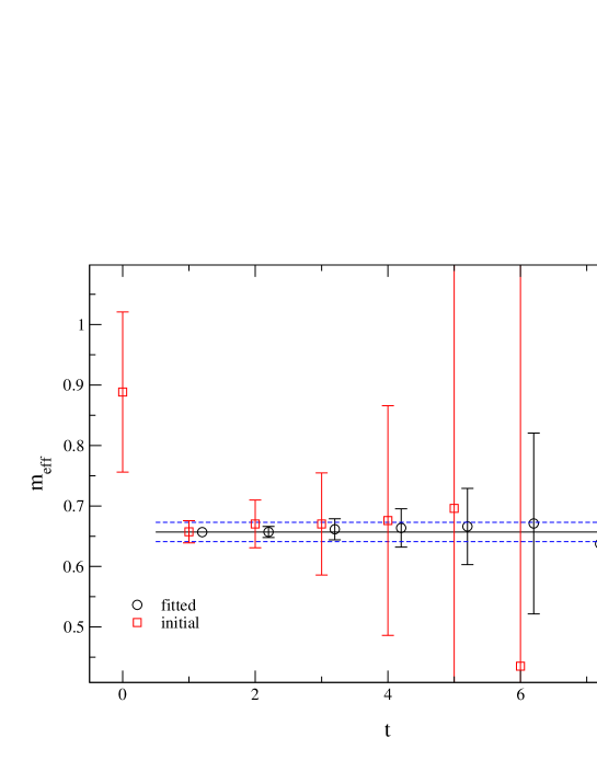
Figure E.1: The effective masses, as defined in eq. E.2, before (squares) and after (circles) the fitting procedure for the ground state of the scalar glueball on the coarse lattice, at $\xi=2$, $\beta=3.15$. The solid and dashed horizontal lines mark the resulting energy and its error, obtained performing a fit on $t=1,\ldots,7$.

Figure E.2 which displays only the final effective mass plots demonstrates that using anisotropic lattices (even at $\xi=2$) may greatly improve the quality of the results.

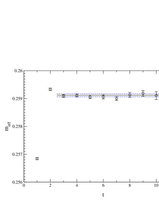
Figure E.2: The effective masses, as defined in eq. E.2 after the fitting procedure for the separation $R=1$ of the on-axis static quark-antiquark potential at $\beta=3.50$.The solid and dashed horizontal lines mark the resulting energy and its error, obtained performing a fit on $t=3,\ldots,12$

E.2 Choosing the Right Mass

In the last Section, we described how one obtains estimates of a state’s mass using sophisticated variational methods, depending on input parameters such as the initial input operators, the number $M$ of operators kept after the first step or the fitting range $t=t_{\text{min}}\ldots t_{\text{max}}$. The number of degrees of freedom in the fit is very large, for typical mass determinations of glueballs it may be of $O(10000)$ if one considers all combinations that might turn out to be sensible, i.e. that might result in a stable mass plateau and a good fit with small $\chi^{2}$.

The first choice one has to make, is the reduction of parameter sets examined to a feasible number, say $O(100)$. This can normally be done quite easily, as the extracted mass should not depend too much on whether, e.g., one chooses $M=13$ or $M=14$, whether one uses the fitting range $t=1\ldots 5$ or $t=1\ldots 6$ etc. Figure E.3 displays the resulting estimates of the full variational method with the condition $\chi^{2}/N_{\text{DF}}<2$ for the ground state of the $A_{1}^{++}$ glueball at $\beta=3.50$ (fixed initial number of operators $N=91$). We have included 16 different fit ranges as well as 11 different truncations $M$. In this case it turns out that it is unambiguous to pick a mass that is consistent with all the determinations, marked by the solid line; the errors of the final result are marked by the dashed lines.

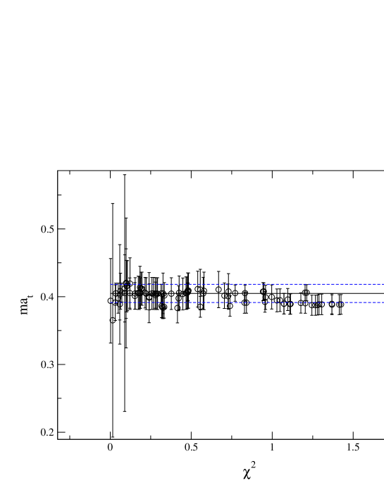
Figure E.3: The mass estimates of the scalar glueball mass on $\xi=2$, $\beta=3.50$ configurations. 16 different fit ranges as well as 11 different truncations $M$ are included. The finally chosen value and its errors are marked by the solid and the dashed lines, respectively.

Of course, the picture does not look that nice in all the cases investigated. Especially for higher masses, where the signal disappears in the noise after just a few time slices, one has to take care to study the behaviour of the mass under the variation of all the parameters and to pick a region where the mass is stable for all sensible choices of parameters. If this is not possible, one might specify an average mass estimate with an error that comprises all the mass estimates coming from sensible choices of the parameters. However, in this case, the error normally gets very large.

Appendix F Representations of Two-Glueball States

In this Appendix we aim at calculating the representation of the cubic group $O_{h}$ to which a pair of glueballs $(\Gamma_{1}^{PC},\Gamma_{2}^{P^{\prime}C^{\prime}})$ with opposite momenta $\vec{p},-\vec{p}$ contributes. These results are used to estimate the minimal energies of glueball pairs on the lattice appearing in each representation, see Section 6.5. The method has been described by Morningstar and Peardon in [18] and is presented in more detail in the following.

F.1 Point Groups Used

Glueballs at rest transform according to the full cubic group $O_{h}$, see Section 2.4.2. This group describes the symmetries of a cube (see Figure F.1) and contains 48 elements in 10 classes: the identity $E$, 8 three-fold ($120^{\circ}$) rotations $C_{3}$, 3 two-fold rotations ($180^{\circ}$) $C_{2}$ around the $x,y,z$-axes, 6 two-fold rotations $C_{2}$ around the axes $a$–$f$ and 6 four-fold rotations ($90^{\circ}$) $C_{4}$; the other five classes contain the same elements, each preceeded by the spatial inversion $I$.

Figure F.1: The rotation axes $Oa,Ob,Oc,Od,Oe,Of,Ox,Oy,Oz,O\alpha,O\beta,O\gamma$ and $O\delta$ of the cubic group $O_{h}$.

Momentum breaks full $O_{h}$ symmetry. Depending on the orientation of the spatial momentum, different symmetries are preserved, the so-called little groups, subgroups of $O_{h}$, describing these remnant symmetries are listed in Table F.1. The group $C_{4v}$ has the symmetries of a regular 4-sided pyramid and contains 8 elements; accordingly the groups $C_{2v}$ and $C_{3v}$ have the symmetries of 2- and 3- sided pyramids respectively and contain 4 and 6 elements. The little group $C_{s}$ contains only two operations, namely the identity $E$ and a mirror reflection $\sigma$; the trivial group $C_{1}$ includes only the identity $E$.

$(n_{x},n_{y},n_{z})$	little group	international notation
(0,0,0)	$O_{h}$	$\frac{4}{m}\bar{3}\frac{2}{m}$
(0,0,n)	$C_{4v}$	$4mm$
(0,n,n)	$C_{2v}$	$2mm$
(n,n,n)	$C_{3v}$	$3m$
(0,m,n)	$C_{s}$	$m$
(m,m,n)	$C_{s}$	$m$
(l,m,n)	$C_{1}$	$1$

Table F.1: The little groups for lattice glueball states having momentum $\vec{p}=2\pi(n_{x},n_{y},n_{z})/S$ on a simple cubic spatial lattice with periodic boundary conditions. Note, that $l,m,n\neq 0$, $l\neq m,m\neq n,l\neq n$. The group $C_{s}$ is often denoted as $S_{1}$. The international notation for the groups is given together with the usual Schoenflies notation for convenience.

F.2 The Method

In order to work out the representations of $O_{h}$ a pair of glueballs with net zero momentum is contributing to, (1) we subduce the given representations of $O_{h}$, $\Gamma_{1}^{PC}$ and $\Gamma_{2}^{P^{\prime}C^{\prime}}$, into the little group under consideration (depending on the momentum orientation). These representations which in general are reducible are then (2) decomposed into direct sums of irreducible representations of the little group. Out of these sums, (3) we build pairs of irreducible representations each coming from one of the initial glueball representations and build their direct product. The direct product is again decomposed into irreducible representations of the little group, and finally, (4) the representation is induced back to $O_{h}$ and decomposed into irreducible representations of this group. That this is possible follows from the net zero momentum of the glueball pairs. In the following, we describe each of these steps in detail.

First, let us introduce the most important tool that will be used, namely characters. The sum of all eigenvalues of a matrix representation $D(G_{a})$ of the group element $G_{a}$, called the character $\chi(G_{a})$, is invariant under similarity transformations $D^{\prime}(G_{a})=AD(G_{a})A^{-1}$. Furthermore, all the elements of a class $\mathcal{C}_{p}$ of a group have the same character $\chi_{p}$, because

$$\chi(G_{a}) \equiv \sum_{i}D_{ii}(G_{a})=\sum_{i}D_{ii}(G_{m}G_{b}G_{m}^{-1})$$ (F.1)

$$= \sum_{ijk}D_{ij}(G_{m})D_{jk}(G_{b})D_{ki}(G_{m}^{-1})$$

$$= \sum_{jk}D_{jk}(G_{b})D_{kj}(G_{m}^{-1}G_{m})$$

$$= \sum_{j}D_{jj}(G_{b})\equiv\chi(G_{b}).$$

The characters of the classes of all the point groups used here are given in Tables F.2, F.5, F.8, F.11, F.14, F.17.

These characters are very useful if one is reducing a representation, i.e. decomposing a given (reducible) representation into its irreducible contents

$$D=\bigoplus_{\alpha}m_{\alpha}T^{(\alpha)},$$ (F.2)

where $\alpha$ runs only over the inequivalent irreducible representations (irreps) $T^{(\alpha)}$ and $m_{\alpha}$ gives the number that this irrep occurs in the reduction. The character of the reducible representation $D$ is related to the irreducible characters $\chi_{p}^{(\alpha)}$ by a similar equation:

$$\chi_{p}=\sum_{\alpha}m_{\alpha}\chi_{p}^{(\alpha)}.$$ (F.3)

The vital task of deducing the coefficients $m_{\alpha}$ given the representation $D$ is facilitated a lot by the use of characters. Using the orthogonality between different irreducible representations, one may show

$$\frac{1}{g}\sum_{p}c_{p}\chi_{p}^{(\beta)*}\chi_{p}=\frac{1}{g}\sum_{\alpha}m_{\alpha}\sum_{p}c_{p}\chi_{p}^{(\beta)*}\chi_{p}^{(\alpha)}=\frac{1}{g}\sum_{\alpha}m_{\alpha}g\delta_{\alpha\beta}=m_{\beta},$$ (F.4)

where $g$ is the order of the group, $c_{p}$ denotes the number of elements in a given class, $p$ runs over the number of classes whereas $\alpha$ numbers the irreps. The coefficient $m_{\beta}$ is thus just the scalar product of the character $\chi$ of the reducible representation with $\chi^{(\beta)}$, the character of the irrep.

Having prepared the most important tools, we may now start to apply the method step by step. As a random example, we study the glueball pair $(T_{1}^{++},A_{1}^{--})$ with momenta $p=\pm 2\pi/S(1,1,1)$.

F.2.1 The Subduction into the Little Group

First, we subduce the characters of $O_{h}$ into the little group under consideration. This amounts to simply picking the right columns out of Table F.2 corresponding to the remnant symmetry operations in the little group under consideration. These correspondences are listed in Table F.4. For our example, with the little group $C_{3v}$, we pick the columns denoted by $E$, $8C_{3}$ and $6IC_{2}$ corresponding to the classes $E$, $2C_{3}$ and $3\sigma_{v}$ of the little group.

F.2.2 The Decomposition into Irreps

The subduced representations, denoted by $O_{h}\downarrow G_{l}$, where $G_{l}$ denotes the little group, are in general reducible in $G_{l}$. Applying eq. F.4 to the subduced characters and the respective characters of the little group, we obtain the decomposition of all the initial representations into the irreps of the little groups, listed in Tables F.7, F.10, F.13, F.16, F.18. For our example groups, we build the scalar products of the subduced characters of $O_{h}$ prepared in the last section and the characters of $C_{3v}$ listed in Table F.11 obtaining Table F.13.

F.2.3 Building Glueball Pairs

Up to now, the steps performed referred to single glueballs having momentum $\vec{p}$. In order to obtain physical objects transforming the same way as our single zero-momentum glueballs, we will now combine two glueballs of opposite momentum. This can be obviously done in the little group corresponding to the momentum. A pair of glueballs transforms according to the direct product of two irreps. On the level of characters this amounts to multiplying the characters of the irreps corresponding to the same group elements (or class). Having in general reducible representations of the initial representations decomposed into irreps, there may be several direct products to be taken into account. In our example, $T_{1}^{++}\downarrow C_{3v}=A_{2}\oplus E$ and $A_{1}^{--}\downarrow C_{3v}=A_{2}$. This leaves us with the direct products $A_{2}\otimes A_{2}$ and $E\otimes A_{2}$. Calculating the characters, one notices easily that $A_{2}\otimes A_{2}=A_{1}$ and $E\otimes A_{2}=E$. That the direct products are irreducible is true for most of the cases; for the other cases, the reduction can be performed exactly the same way as presented in Section F.2 and applied in Section F.2.2. For convenience, the multiplication tables (together with the decomposition into irreps) are given as Tables F.3, F.6, F.9, F.12, F.15 (the table for the group $C_{1}$ is completely trivial and thus omitted).

In the case of both glueballs having momentum 0, i.e. transforming according to $O_{h}$, the whole method amounts to simply performing the direct products and reading off the resulting irreps of $O_{h}$ in Table F.3.

F.2.4 The Induction back to the Cubic Group

For most of the representations of the glueball pairs in the little groups, the induction (getting back onto the level of the full cubic group $O_{h}$) is trivial, due to the Frobenius reciprocity theorem that states that the number of times a representation $D^{(\nu)}(G)$ occurs in $D^{(\mu)}\uparrow G$, the induced representation, is equal to the number of occurrences of the irrep $D^{(\mu)}(G_{s})$ in $D^{(\nu)}\downarrow G_{s}$, i.e. if the representation of the glueball pair in the little group is again an irrep of the little group, we can read off the contents of the induced representation in terms of the irreps of $O_{h}$ again from Tables F.7, F.10, F.13, F.16, F.18.

For the two cases ($E\otimes E$ in $C_{4v}$ and $E\otimes E$ in $C_{3v}$) where the direct product is not an irrep of the little group, we just give the results: $(E\otimes E)\uparrow O_{h}=E^{+}\oplus E^{-}$ for $C_{4v}$, whereas $E\otimes E$ contributes to all representations of $O_{h}$ for $C_{3v}$. The way of performing these inductions is employing the left coset decomposition of $O_{h}$ in terms of the little group, see e.g. [158, 159].

In our example, the irreps of the little group describing the glueball pair are $A_{1}$ and $E$. Using the Frobenius theorem with Table F.13 , we notice easily that the pair may contribute to the irreps $A_{1}^{+},E^{+},T_{1}^{+},T_{2}^{+},A_{2}^{-},E^{-},T_{1}^{-},T_{2}^{-}$ of the cubic group $O_{h}$.

F.2.5 A Note on Parity and Charge Conjugation

In the previous sections, the parity quantum number $P=\pm$ we have always taken into account, whereas the charge conjugation $C$ has been omitted. The reason for this is simple: once the momentum of a single glueball is non-zero, it is no longer an eigenstate of parity, i.e. that is why we have to consider the decomposition into irreps of the little groups for $P=+$ and $P=-$ states separately. Charge conjugation is completely different: the quantum number $C_{2}$ of the glueball pair is always just the product $C\cdot C^{\prime}$ of the quantum numbers of the initial states, therefore the results for $C=C^{\prime}=+$ can be trivially generalised to the other three cases.

There is another important issue concerning parity, namely if the two glueballs are indistinguishable (having the same $\Gamma^{PC}$), the final two-glueball state has to have positive parity due to the Bose-symmetry. Hypothetic $P=-$ glueball pairs consisting of two states having the same quantum numbers thus have to be excluded.

For our example, all this means that because of the two representations, $T_{1}^{++}$ and $A_{1}^{--}$, being different, Bose symmetry does not exclude any states; furthermore that the resulting states have charge conjugation quantum number $C=-$. The two glueballs of our example, having momenta $\vec{p}$ parallel to the space diagonal thus contribute to the representations $A_{1}^{+-}$, $E^{+-}$, $T_{1}^{+-}$, $T_{2}^{+-}$, $A_{2}^{--}$, $E^{--}$, $T_{1}^{--}$, $T_{2}^{--}$.

F.3 Results

We calculate the energies of all possible glueball pairs on all our lattices for momenta up to $|\vec{p}|=3\cdot 2\pi/Sa_{s}$. The resulting lowest-lying masses of glueball pairs, for all the representations where states can be measured at a given $\beta$ are given in Tables G.9–G.11. The spectra are displayed in Figures F.2–F.4.

$O_{h}$	$E$	$8C_{3}$	$3C_{2}$	$6C_{2}$	$6C_{4}$	$I$	$8IC_{3}$	$3IC_{2}$	$6IC_{2}$	$6IC_{4}$
$A_{1}^{+}$	1	1	1	1	1	1	1	1	1	1
$A_{2}^{+}$	1	1	1	-1	-1	1	1	1	-1	-1
$E^{+}$	2	-1	2	0	0	2	-1	2	0	0
$T_{1}^{+}$	3	0	-1	-1	1	3	0	-1	-1	1
$T_{2}^{+}$	3	0	-1	1	-1	3	0	-1	1	-1
$A_{1}^{-}$	1	1	1	1	1	-1	-1	-1	-1	-1
$A_{2}^{-}$	1	1	1	-1	-1	-1	-1	-1	1	1
$E^{-}$	2	-1	2	0	0	-2	1	-2	0	0
$T_{1}^{-}$	3	0	-1	-1	1	-3	0	1	1	-1
$T_{2}^{-}$	3	0	-1	1	-1	-3	0	1	-1	1

Table F.2: The character table for the cubic point group $O_{h}$.

$O$	$A_{1}^{+}$	$A_{2}^{+}$	$E^{+}$	$T_{1}^{+}$	$T_{2}^{+}$
$A_{1}^{+}$	$A_{1}^{+}$	$A_{2}^{+}$	$E^{+}$	$T_{1}^{+}$	$T_{2}^{+}$
$A_{2}^{+}$		$A_{1}^{+}$	$E^{+}$	$T_{2}^{+}$	$T_{1}^{+}$
$E^{+}$			$A_{1}^{+}\oplus A_{2}^{+}\oplus E$	$T_{1}^{+}\oplus T_{2}^{+}$	$T_{1}^{+}\oplus T_{2}^{+}$
$T_{1}^{+}$				$A_{1}^{+}\oplus E\oplus T_{1}^{+}\oplus T_{2}^{+}$	$A_{2}^{+}\oplus E\oplus T_{1}^{+}\oplus T_{2}^{+}$
$T_{2}^{+}$					$A_{1}^{+}\oplus E\oplus T_{1}^{+}\oplus T_{2}^{+}$

Table F.3: The direct products of the irreducible representations (irreps) of the cubic point group $O$, decomposed back into direct sums of the irreps. For the (trivial) extension to the full cubic group $O_{h}$, see text. Due to the obvious symmetry, only the upper diagonal part of the table is given.

	$E$	$8C_{3}$	$3C_{2}$	$6C_{2}$	$6C_{4}$	$I$	$8IC_{3}$	$3IC_{2}$	$6IC_{2}$	$6IC_{4}$
$C_{4v}$	$E$		$C_{2}$		$2C_{4}$			$2\sigma_{v}$	$2\sigma_{d}$
$C_{2v}$	$E$			$C_{2}$				$\sigma_{x}$	$\sigma_{y}$
$C_{3v}$	$E$	$2C_{3}$							$3\sigma_{v}$
$C_{s}$	$E$								$\sigma$
$C_{1}$	$E$

Table F.4: The correspondence of the classes of the cubic point group $O_{h}$ to the classes of the little groups $C_{4v},C_{2v},C_{3v},C_{s},C_{1}$.

$C_{4v}$	$E$	$C_{2}$	$2C_{4}$	$2\sigma_{v}$	$2\sigma_{d}$
$A_{1}$	1	1	1	1	1
$A_{2}$	1	1	1	-1	-1
$B_{1}$	1	1	-1	1	-1
$B_{2}$	1	1	-1	-1	1
$E$	2	-2	0	0	0

Table F.5: The character table for the point group $C_{4v}$.

$C_{4v}$	$A_{1}$	$A_{2}$	$B_{1}$	$B_{2}$	$E$
$A_{1}$	$A_{1}$	$A_{2}$	$B_{1}$	$B_{2}$	$E$
$A_{2}$		$A_{1}$	$B_{2}$	$B_{1}$	$E$
$B_{1}$			$A_{1}$	$A_{2}$	$E$
$B_{2}$				$A_{1}$	$E$
$E$					$A_{1}\oplus A_{2}\oplus B_{1}\oplus B_{2}$

Table F.6: The direct products of the irreducible representations (irreps) of the point group $C_{4v}$, decomposed back into direct sums of the irreps. Due to the obvious symmetry, only the upper diagonal part of the table is given.

$O_{h}$ irrep.	$A_{1}$	$A_{2}$	$B_{1}$	$B_{2}$	$E$
$A_{1}^{+}$	1	0	0	0	0
$A_{2}^{+}$	0	0	1	0	0
$E^{+}$	1	0	1	0	0
$T_{1}^{+}$	0	1	0	0	1
$T_{2}^{+}$	0	0	0	1	1
$A_{1}^{-}$	0	1	0	0	0
$A_{2}^{-}$	0	0	0	1	0
$E^{-}$	0	1	0	1	0
$T_{1}^{-}$	1	0	0	0	1
$T_{2}^{-}$	0	0	1	0	1

Table F.7: The decomposition of the subduced representations $O_{h}\downarrow C_{4v}$ in terms of the irreducible representations of the little group.

$C_{2v}$	$E$	$C_{2}$	$\sigma_{y}$	$\sigma_{x}$
$A_{1}$	1	1	1	1
$B_{1}$	1	-1	-1	1
$A_{2}$	1	1	-1	-1
$B_{2}$	1	-1	1	-1

Table F.8: The character table for the point group $C_{2v}$.

$C_{2v}$	$A_{1}$	$B_{1}$	$A_{2}$	$B_{2}$
$A_{1}$	$A_{1}$	$B_{1}$	$A_{2}$	$B_{2}$
$B_{1}$		$A_{1}$	$B_{2}$	$A_{2}$
$A_{2}$			$A_{1}$	$B_{1}$
$B_{2}$				$A_{1}$

Table F.9: The direct products of the irreducible representations (irreps) of the point group $C_{2v}$, decomposed back into direct sums of the irreps. Due to the obvious symmetry, only the upper diagonal part of the table is given.

$O_{h}$ irrep.	$A_{1}$	$B_{1}$	$A_{2}$	$B_{2}$
$A_{1}^{+}$	1	0	0	0
$A_{2}^{+}$	0	1	0	0
$E^{+}$	1	1	0	0
$T_{1}^{+}$	0	1	1	1
$T_{2}^{+}$	1	0	1	1
$A_{1}^{-}$	0	0	1	0
$A_{2}^{-}$	0	0	0	1
$E^{-}$	0	0	1	1
$T_{1}^{-}$	1	1	0	1
$T_{2}^{-}$	1	1	1	0

Table F.10: The decomposition of the subduced representations $O_{h}\downarrow C_{2v}$ in terms of the irreducible representations of the little group.

$C_{3v}$	$E$	$2C_{3}$	$3\sigma_{v}$
$A_{1}$	1	1	1
$A_{2}$	1	1	-1
$E$	2	-1	0

Table F.11: The character table for the point group $C_{3v}$.

$C_{3v}$	$A_{1}$	$A_{2}$	$E$
$A_{1}$	$A_{1}$	$A_{2}$	$E$
$A_{2}$		$A_{1}$	$E$
$E$			$A_{1}\oplus A_{2}\oplus E$

Table F.12: The direct products of the irreducible representations (irreps) of the point group $C_{3v}$, decomposed back into direct sums of the irreps. Due to the obvious symmetry, only the upper diagonal part of the table is given.

$O_{h}$ irrep.	$A_{1}$	$A_{2}$	$E$
$A_{1}^{+}$	1	0	0
$A_{2}^{+}$	0	1	0
$E^{+}$	0	0	1
$T_{1}^{+}$	0	1	1
$T_{2}^{+}$	0	1	1
$A_{1}^{-}$	0	1	0
$A_{2}^{-}$	1	0	0
$E^{-}$	0	0	1
$T_{1}^{-}$	1	0	1
$T_{2}^{-}$	1	0	1

Table F.13: The decomposition of the subduced representations $O_{h}\downarrow C_{3v}$ in terms of the irreducible representations of the little group.

$C_{s}$	$E$	$\sigma$
$A_{1}$	1	1
$A_{2}$	1	-1

Table F.14: The character table for the point group $C_{s}$.

$C_{s}$	$A_{1}$	$A_{2}$
$A_{1}$	$A_{1}$	$A_{2}$
$A_{2}$	$A_{2}$	$A_{1}$

Table F.15: The direct products of the irreducible representations (irreps) of the point group $C_{s}$, decomposed back into direct sums of the irreps.

$O_{h}$ irrep.	$A_{1}$	$A_{2}$
$A_{1}^{+}$	1	0
$A_{2}^{+}$	0	1
$E^{+}$	1	1
$T_{1}^{+}$	1	2
$T_{2}^{+}$	2	1
$A_{1}^{-}$	0	1
$A_{2}^{-}$	1	0
$E^{-}$	1	1
$T_{1}^{-}$	2	1
$T_{2}^{-}$	1	2

Table F.16: The decomposition of the subduced representations $O_{h}\downarrow C_{s}$ in terms of the irreducible representations of the little group.

$C_{1}$	$E$
$A_{1}$	1

Table F.17: The character table for the point group $C_{1}$.

$O_{h}$ irrep.	$A_{1}$
$A_{1}^{+}$	1
$A_{2}^{+}$	1
$E^{+}$	2
$T_{1}^{+}$	3
$T_{2}^{+}$	3
$A_{1}^{-}$	1
$A_{2}^{-}$	1
$E^{-}$	2
$T_{1}^{-}$	3
$T_{2}^{-}$	3

Table F.18: The decomposition of the subduced representations $O_{h}\downarrow C_{1}$ in terms of the irreducible representations of the little group.

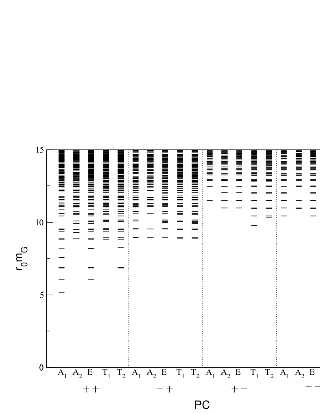
Figure F.2: The two-glueball spectrum on the $\beta=3.15$ lattice.

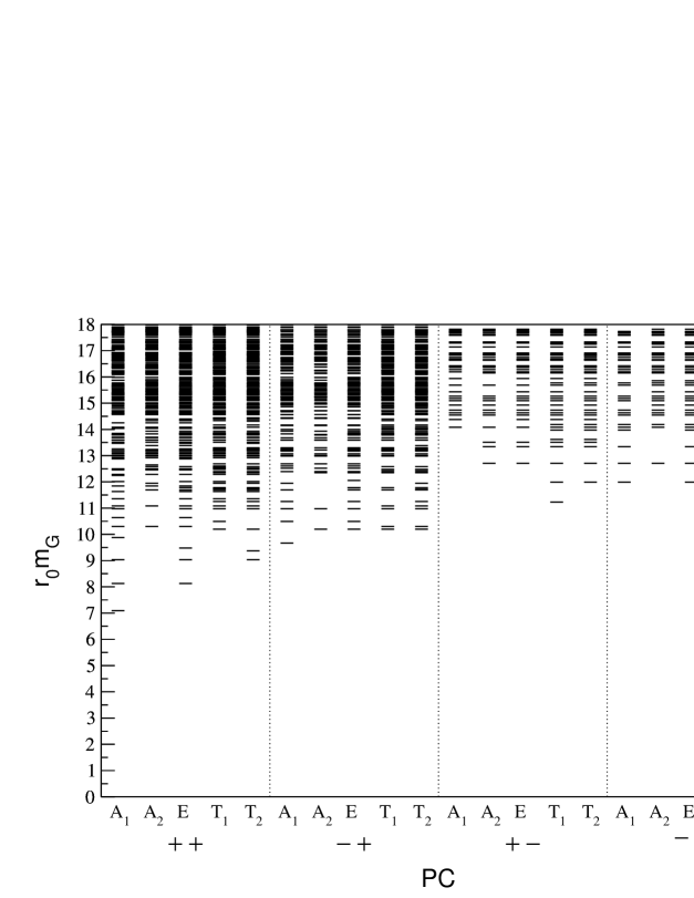
Figure F.3: The two-glueball spectrum on the $\beta=3.30$ lattice.

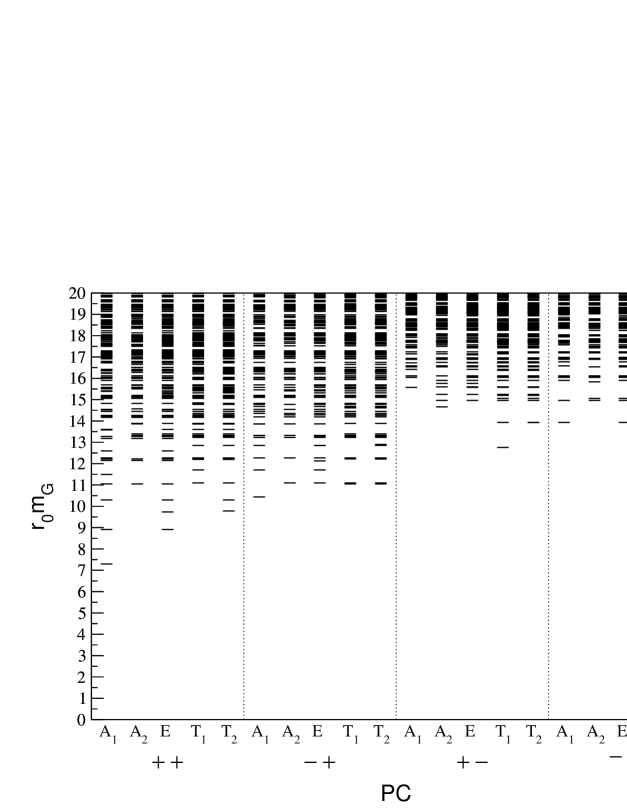
Figure F.4: The two-glueball spectrum on the $\beta=3.50$ lattice.

Appendix G Collection of Results

$\beta$	$p^{2}$	$M$	fit range	$a_{t}E(p^{2})$	$\chi^{2}/N_{\text{DF}}$
3.0	0	2	1–5	1.368(30)	0.19
	1	3	1–6	1.372(17)	0.49
	2	3	1–6	1.451(17)	0.28
	4	3	1–8	1.570(21)	0.46
	5	3	1–6	1.610(19)	0.34
	8	2	1–3	1.707(29)	0.05
3.15a	0	3	2–5	0.688(16)	0.11
	1	4	1–5	0.806(5)	0.06
	2	4	1–5	0.902(6)	0.59
	4	3	1–5	1.059(8)	2.35
	5	4	1–5	1.151(7)	0.16
	8	4	1–5	1.310(15)	0.71
	9	4	1–5	1.356(23)	1.58
	10	4	1–3	1.470(17)	0.42
	13	3	1–3	1.621(23)	0.01
	18	3	1–3	1.762(47)	0.56
3.15b	1	3	1–5	1.418(23)	0.05
	2	3	1–5	1.541(37)	0.53
	4	3	1–4	1.751(67)	1.20
	5	3	1–5	1.922(104)	1.08

Table G.1: Collection of results of the torelon measurements using the $\xi=2$ perfect action. For each $\beta$-value and momentum $p^{2}=p_{x}^{2}+p_{y}^{2}$ we list the number of operators $M$ kept after the first truncation in the variational method, the plateau region on which the fit of the correlators to the form $Z(p^{2})\exp(-tE(p^{2}))$ is performed (fit range), as well as the extracted energy together with the $\chi^{2}$ per degree of freedom ($\chi^{2}/N_{\text{DF}}$). (Continued in Table G.2)

$\beta$	$p^{2}$	$M$	fit range	$a_{t}E(p^{2})$	$\chi^{2}/N_{\text{DF}}$
3.3	0	3	1–10	0.318(6)	1.39
	1	3	1–10	0.417(3)	1.20
	2	3	1–5	0.493(3)	0.13
	4	4	1–4	0.633(4)	1.26
	5	5	1–10	0.688(3)	0.84
	8	5	1–8	0.830(5)	1.21
	9	5	1–6	0.877(6)	0.42
	10	5	1–10	0.921(4)	0.77
	13	5	1–10	1.036(6)	0.30
	18	4	1–6	1.205(12)	0.15
3.5a	1	5	3–8	0.305(6)	0.10
	2	5	1–10	0.407(4)	1.65
	4	4	1–10	0.538(4)	0.96
	5	5	1–10	0.586(3)	1.16
	8	5	1–7	0.721(4)	0.09
	9	5	2–6	0.733(10)	0.11
	10	4	1–8	0.795(4)	0.96
	13	5	1–6	0.901(4)	1.26
	18	5	1–6	1.058(9)	1.45
3.5b	1	4	3–7	0.321(5)	1.00
	2	5	1–8	0.432(3)	0.81
	4	5	1–8	0.586(4)	0.29
	5	5	1–7	0.656(3)	1.24
	8	5	2–7	0.806(14)	0.36
	9	5	1–7	0.859(7)	0.74
	10	5	1–8	0.913(4)	0.68
	13	5	2–5	1.010(16)	0.32
	18	3	1–5	1.215(12)	0.17

Table G.2: Collection of results of the torelon measurements using the $\xi=2$ perfect action. For each $\beta$-value and momentum $p^{2}=p_{x}^{2}+p_{y}^{2}$ we list the number of operators $M$ kept after the first truncation in the variational method, the plateau region on which the fit of the correlators to the form $Z(p^{2})\exp(-tE(p^{2}))$ is performed (fit range), as well as the extracted energy together with the $\chi^{2}$ per degree of freedom ($\chi^{2}/N_{\text{DF}}$). (Continuation from Table G.1)

$\vec{r}$	$|\vec{r}|$	$M$	fit range	$a_{t}V(\vec{r})$	$\chi^{2}/N_{\text{DF}}$
(1,0,0)	1	3	2–7	0.5053(3)	0.70
(1,1,0)	1.414	3	3–5	0.7322(7)	0.01
(1,1,1)	1.732	3	3–8	0.8902(14)	0.60
(2,0,0)	2	3	2–8	0.9407(10)	0.89
(2,1,0)	2.236	3	2–8	1.0642(11)	0.36
(2,1,1)	2.449	2	2–5	1.1676(13)	0.27
(2,2,0)	2.828	3	2–6	1.3082(18)	0.17
(3,0,0)	3	3	2–6	1.3392(25)	0.16
(2,2,1)	3	3	2–5	1.3867(20)	0.26
(2,2,2)	3.464	3	2–6	1.5675(55)	0.84
(4,0,0)	4	2	1–5	1.7429(24)	0.14
(4,2,0)	4.472	3	2–6	1.9328(93)	1.47
(4,2,2)	4.899	3	1–4	2.1197(34)	0.15

Table G.3: Collection of results of the off-axis $q\bar{q}$ measurements using the $\xi=2$ perfect action at $\beta=3.00$. For each separation vector we list the length of the vector in spatial lattice units, the number of operators $M$ kept after the first truncation in the variational method, the plateau region on which the fit of the correlators to the form $Z(\vec{r})\exp(-tE(\vec{r}))$ is performed (fit range), as well as the extracted energy together with the $\chi^{2}$ per degree of freedom ($\chi^{2}/N_{\text{DF}}$).

$\vec{r}$	$|\vec{r}|$	$M$	fit range	$a_{t}V(\vec{r})$	$\chi^{2}/N_{\text{DF}}$
(1,0,0)	1	3	3–10	0.3006(1)	0.20
(1,1,0)	1.414	3	3–10	0.3814(2)	0.21
(1,1,1)	1.732	3	3–10	0.4250(3)	0.65
(2,0,0)	2	3	6–10	0.4469(6)	0.22
(2,1,0)	2.236	3	4–10	0.4752(4)	0.41
(2,1,1)	2.449	3	4–10	0.4971(5)	0.83
(2,2,0)	2.828	3	4–10	0.5309(7)	0.59
(3,0,0)	3	3	4–10	0.5445(7)	1.71
(2,2,1)	3	3	5–10	0.5456(8)	0.62
(2,2,2)	3.464	3	4–10	0.5852(9)	1.53
(4,0,0)	4	3	4–10	0.6269(1)	0.51
(3,3,0)	4.243	3	5–10	0.6455(16)	0.94
(4,2,0)	4.472	3	5–10	0.6630(14)	0.86
(4,2,2)	4.899	3	5–10	0.6964(18)	0.34
(5,0,0)	5	2	5–10	0.7044(22)	1.24
(3,3,3)	5.196	3	4–10	0.7215(17)	1.31
(4,4,0)	5.657	2	6–10	0.7509(41)	1.23
(4,4,2)	6	3	5–10	0.7783(25)	0.77

Table G.4: Collection of results of the off-axis $q\bar{q}$ measurements using the $\xi=2$ perfect action at $\beta=3.30$. For each separation vector we list the length of the vector in spatial lattice units, the number of operators $M$ kept after the first truncation in the variational method, the plateau region on which the fit of the correlators to the form $Z(\vec{r})\exp(-tE(\vec{r}))$ is performed (fit range), as well as the extracted energy together with the $\chi^{2}$ per degree of freedom ($\chi^{2}/N_{\text{DF}}$).

$\beta$	$r$	$M$	fit range	$a_{t}V(r)$	$\chi^{2}/N_{\text{DF}}$
3.15	1	5	3–10	0.3703(2)	0.456
	2	5	3–7	0.6110(4)	0.735
	3	5	3–10	0.8019(8)	1.209
	4	5	3–7	0.9775(16)	1.238
	5	5	4–9	1.129(8)	0.519
3.50	1	5	3–12	0.25910(5)	1.163
	2	5	3–10	0.36490(12)	0.769
	3	5	7–12	0.42168(38)	0.664
	4	5	5–11	0.46587(51)	0.205
	5	5	5–12	0.50388(76)	1.139
	6	5	5–11	0.54051(96)	0.853

Table G.5: Collection of results of the on-axis $q\bar{q}$ measurements using the $\xi=2$ perfect action at $\beta=$ 3.15, 3.50. For each separation along the axes we list the number of operators $M$ kept after the first truncation in the variational method, the plateau region on which the fit of the correlators to the form $Z(r)\exp(-tE(r))$ is performed (fit range), as well as the extracted energy together with the $\chi^{2}$ per degree of freedom ($\chi^{2}/N_{\text{DF}}$).

Channel	$N$	$t_{0}/t_{1}$	$M$	fit range	$\chi^{2}/N_{\text{DF}}$	energies
$A_{1}^{++}$	87	1/2	12	1 – 4	0.69	0.645(10)
${A_{1}^{++}}^{*}$	59	1/2	10	1 – 3	1.23	1.365(104)
$E^{++}$	47	1/2	7	1 – 3	0.10	1.405(29)
${E^{++}}^{*}$	47	1/2	5	1 – 3	0.17	1.985(140)
$T_{2}^{++}$	47	1/2	10	1 – 4	0.10	1.416(32)
${T_{2}^{++}}^{*}$	22	1/2	6	1 – 3	1.20	1.990(131)
$A_{2}^{++}$	21	1/2	2	1 – 3	0.03	1.675(147)
$T_{1}^{++}$	36	1/2	4	1 – 3	0.34	1.881(131)
${T_{1}^{++}}^{*}$	36	1/2	6	1 – 3	0.31	2.170(182)
$A_{1}^{-+}$	25	1/2	3	1 – 3	0.001	1.588(114)
$E^{-+}$	25	1/2	2	1 – 3	0.01	1.849(81)
${E^{-+}}^{*}$	25	1/2	2	1 – 3	2.19	2.084(268)
$T_{2}^{-+}$	64	1/2	4	1 – 3	0.02	1.850(83)
$T_{1}^{+-}$	61	1/2	4	1 – 3	0.24	1.798(59)
$T_{2}^{+-}$	18	1/2	4	1 – 3	0.41	1.935(177)

Table G.6: Results from fits to the $\xi=2$, $\beta=3.15$ glueball correlators on the $8^{3}\times 16$ lattice in units of the temporal lattice spacing $a_{t}$: $t_{0}$/$t_{1}$ are used in the generalised eigenvalue problem, $N$ is the number of initial operators measured and $M$ denotes the number of operators kept after the truncation in $C(t_{0})$.

Channel	$t_{0}/t_{1}$	$M$	fit range	$\chi^{2}/N_{\text{DF}}$	energies
$A_{1}^{++}$	1/2	9	2 – 7	0.90	0.590(17)
${A_{1}^{++}}^{*}$	1/2	11	1 – 3	1.57	1.133(53)
$E^{++}$	1/2	11	1 – 5	0.97	0.983(17)
${E^{++}}^{*}$	1/2	8	1 – 3	0.90	1.453(68)
$T_{2}^{++}$	1/2	12	1 – 4	1.09	0.965(15)
${T_{2}^{++}}^{*}$	1/2	10	1 – 4	1.68	1.386(51)
$A_{2}^{++}$	1/2	4	1 – 3	0.01	1.511(94)
$T_{1}^{++}$	1/2	8	1 – 5	0.84	1.492(62)
$A_{1}^{-+}$	1/2	6	1 – 4	4.38	1.017(39)
$E^{-+}$	1/2	3	1 – 4	0.74	1.365(36)
$T_{2}^{-+}$	1/2	4	1 – 5	1.16	1.357(25)
$T_{1}^{+-}$	1/2	8	1 – 4	0.95	1.276(33)

Table G.7: Results from fits to the $\xi=2$, $\beta=3.3$ glueball correlators on the $10^{3}\times 20$ lattice in units of the temporal lattice spacing $a_{t}$: $t_{0}$/$t_{1}$ are used in the generalised eigenvalue problem, $M$ denotes the number of operators kept after the truncation in $C(t_{0})$.

Channel	$N$	$t_{0}/t_{1}$	$M$	fit range	$\chi^{2}/N_{\text{DF}}$	energies
$A_{1}^{++}$	91	1/2	24	2 – 7	0.31	0.405(13)
${A_{1}^{++}}^{*}$	110	0/1	110	4 – 6	0.30	0.720(158)
$E^{++}$	104	1/2	23	2 – 5	0.16	0.675(25)
${E^{++}}^{*}$	104	1/2	14	1 – 3	0.70	1.183(55)
$T_{2}^{++}$	53	1/2	19	2 – 5	0.31	0.681(12)
${T_{2}^{++}}^{*}$	53	1/2	22	1 – 3	0.69	1.128(23)
$A_{2}^{++}$	15	1/2	6	1 – 3	0.05	1.212(42)
${A_{2}^{++}}^{*}$	15	1/2	6	1 – 3	1.12	1.568(130)
$T_{1}^{++}$	23	1/2	11	1 – 4	0.05	1.245(25)
$A_{1}^{-+}$	15	1/2	9	1 – 3	0.17	0.754(23)
${A_{1}^{-+}}^{*}$	15	1/2	9	1 – 3	0.61	1.140(112)
$E^{-+}$	21	1/2	14	1 – 3	0.27	0.942(24)
${E^{-+}}^{*}$	21	1/2	11	1 – 3	1.20	1.406(80)
$T_{2}^{-+}$	75	1/2	9	2 – 5	0.32	0.952(38)
${T_{2}^{-+}}^{*}$	75	1/2	6	1 – 3	1.70	1.675(59)
$T_{1}^{+-}$	53	1/2	14	1 – 3	0.69	1.013(17)
$A_{2}^{+-}$	11	1/2	5	1 – 3	0.07	1.224(64)
${A_{2}^{+-}}^{*}$	11	1/2	5	1 – 3	0.79	1.726(147)
$T_{2}^{+-}$	22	1/2	9	2 – 4	0.33	1.142(121)
${T_{2}^{+-}}^{*}$	12	1/2	9	1 – 3	1.78	1.663(139)
$E^{+-}$	50	0/1	50	1 – 3	1.01	1.379(34)
$T_{1}^{--}$	80	0/1	80	2 – 4	0.57	1.200(67)
$T_{2}^{--}$	80	0/1	80	2 – 5	0.20	1.205(81)
$A_{2}^{--}$	35	0/1	35	1 – 3	0.16	1.352(37)
$A_{1}^{--}$	30	0/1	30	1 – 4	0.14	1.703(99)

Table G.8: Results from fits to the $\xi=2$, $\beta=3.5$ glueball correlators on the $12^{3}\times 24$ lattice in units of the temporal lattice spacing $a_{t}$: $t_{0}$/$t_{1}$ are used in the generalised eigenvalue problem, $N$ is the number of initial operators measured and $M$ denotes the number of operators kept after the truncation in $C(t_{0})$.

Channel	Glueballs	$p^{2}$	$r_{0}\cdot m_{2G}$
$A_{1}^{++}$	($A_{1}^{++}$, $A_{1}^{++}$)	0	5.16
$E^{++}$	($A_{1}^{++}$, $A_{1}^{++}$)	1	6.07
$T_{2}^{++}$	($A_{1}^{++}$, $A_{1}^{++}$)	2	6.86
$A_{2}^{++}$	($A_{1}^{++}$, $E^{++}$)	1	8.89
$T_{1}^{++}$	($A_{1}^{++}$, $A_{1}^{++}$)	5	8.82
$A_{1}^{-+}$	($A_{1}^{++}$, $A_{1}^{-+}$)	0	8.94
$E^{-+}$	($A_{1}^{++}$, $T_{2}^{++}$)	1	8.93
$T_{2}^{-+}$	($A_{1}^{++}$, $E^{++}$)	1	8.89
$T_{1}^{+-}$	($A_{1}^{++}$, $T_{1}^{+-}$)	0	9.78
$T_{2}^{+-}$	($A_{1}^{++}$, $T_{2}^{+-}$)	0	10.33

Table G.9: The energies of the lowest-lying two-glueball states with zero momentum for all the symmetry channels, given in terms of $r_{0}$, using the masses determined in the $\beta=3.15$ simulation. The square of the momenta $p^{2}$ of the single glueballs building the pair is given in units of $(2\pi/8a_{s})^{2}=(1.60/r_{0})^{2}$.

Channel	Glueballs	$p^{2}$	$r_{0}\cdot m_{2G}$
$A_{1}^{++}$	($A_{1}^{++}$, $A_{1}^{++}$)	0	7.10
$E^{++}$	($A_{1}^{++}$, $A_{1}^{++}$)	1	8.13
$T_{2}^{++}$	($A_{1}^{++}$, $A_{1}^{++}$)	2	9.04
$A_{2}^{++}$	($A_{1}^{++}$, $E^{++}$)	1	10.32
$T_{1}^{++}$	($A_{1}^{++}$, $T_{2}^{++}$)	1	10.21
$A_{1}^{-+}$	($A_{1}^{++}$, $A_{1}^{-+}$)	0	9.68
$E^{-+}$	($A_{1}^{++}$, $T_{2}^{++}$)	1	10.21
$T_{2}^{-+}$	($A_{1}^{++}$, $T_{2}^{++}$)	1	10.21
$T_{1}^{+-}$	($A_{1}^{++}$, $T_{1}^{+-}$)	0	11.24

Table G.10: The energies of the lowest-lying two-glueball states with zero momentum for all the symmetry channels, given in terms of $r_{0}$, using the masses determined in the $\beta=3.30$ simulation. The square of the momenta $p^{2}$ of the single glueballs building the pair is given in units of $(2\pi/10a_{s})^{2}=(1.98/r_{0})^{2}$.

Channel	Glueballs	$p^{2}$	$r_{0}\cdot m_{2G}$
$A_{1}^{++}$	($A_{1}^{++}$, $A_{1}^{++}$)	0	7.30
$E^{++}$	($A_{1}^{++}$, $A_{1}^{++}$)	1	8.93
$T_{2}^{++}$	($A_{1}^{++}$, $T_{2}^{++}$)	0	9.78
$A_{2}^{++}$	($A_{1}^{++}$, $E^{++}$)	1	11.06
$T_{1}^{++}$	($A_{1}^{++}$, $T_{2}^{++}$)	1	11.11
$A_{1}^{-+}$	($A_{1}^{++}$, $A_{1}^{-+}$)	0	10.44
$E^{-+}$	($A_{1}^{++}$, $T_{2}^{++}$)	1	11.11
$T_{2}^{-+}$	($A_{1}^{++}$, $E^{++}$)	1	11.06
$T_{1}^{+-}$	($A_{1}^{++}$, $T_{1}^{+-}$)	0	12.77
$A_{2}^{+-}$	($A_{1}^{++}$, $A_{2}^{+-}$)	0	14.67
$T_{2}^{+-}$	($A_{1}^{++}$, $T_{2}^{+-}$)	0	13.94
$E^{+-}$	($A_{1}^{++}$, $T_{1}^{+-}$)	2	14.97
$T_{1}^{--}$	($A_{1}^{++}$, $T_{1}^{+-}$)	1	13.94
$T_{2}^{--}$	($A_{1}^{++}$, $T_{1}^{+-}$)	1	13.94
$A_{2}^{--}$	($A_{1}^{++}$, $T_{1}^{+-}$)	2	14.97
$A_{1}^{--}$	($A_{1}^{++}$, $T_{1}^{+-}$)	1	13.94

Table G.11: The energies of the lowest-lying two-glueball states with zero momentum for all the symmetry channels, given in terms of $r_{0}$, using the masses determined in the $\beta=3.50$ simulation. The square of the momenta $p^{2}$ of the single glueballs building the pair is given in units of $(2\pi/12a_{s})^{2}=(2.57/r_{0})^{2}$.

Ratio	$\beta=3.15$	$\beta=3.30$	$\beta=3.50$
$m({A_{1}^{++}}^{*})/m({A_{1}^{++}})$	2.12(19)	1.92(15)	1.78(45)
$m({E^{++}})/m({A_{1}^{++}})$	2.18(8)	1.67(8)	1.67(12)
$m({E^{++}}^{*})/m({A_{1}^{++}})$	3.08(26)	2.46(19)	2.92(23)
$m({T_{2}^{++}})/m({A_{1}^{++}})$	2.20(8)	1.64(7)	1.68(8)
$m({T_{2}^{++}}^{*})/m({A_{1}^{++}})$	3.09(25)	2.35(15)	2.79(15)
$m({A_{2}^{++}})/m({A_{1}^{++}})$	2.60(27)	2.56(23)	2.99(20)
$m({A_{2}^{++}}^{*})/m({A_{1}^{++}})$			3.87(45)
$m({T_{1}^{++}})/m({A_{1}^{++}})$	2.92(25)	2.53(18)	3.07(16)
$m({A_{1}^{-+}})/m({A_{1}^{++}})$	2.46(21)	1.72(12)	1.86(12)
$m({A_{1}^{-+}}^{*})/m({A_{1}^{++}})$			2.81(37)
$m({E^{-+}})/m({A_{1}^{++}})$	2.87(17)	2.31(13)	2.33(13)
$m({E^{-+}}^{*})/m({A_{1}^{++}})$	3.23(47)		3.47(31)
$m({T_{2}^{-+}})/m({A_{1}^{++}})$	2.87(17)	2.30(11)	2.35(17)
$m({T_{2}^{-+}}^{*})/m({A_{1}^{++}})$			4.14(28)
$m({T_{1}^{+-}})/m({A_{1}^{++}})$	2.79(13)	2.16(12)	2.50(12)
$m({A_{2}^{+-}})/m({A_{1}^{++}})$			3.02(26)
$m({T_{2}^{+-}})/m({A_{1}^{++}})$			2.82(39)

Table G.12: Glueball mass ratios with the scalar glueball mass, $m_{G}/m({A_{1}^{++}})$.

Ratio	$\beta=3.15$	$\beta=3.30$	$\beta=3.50$
$m({A_{1}^{++}})/m({T_{2}^{++}})$	0.46(2)	0.61(3)	0.59(3)
$m({A_{1}^{++}}^{*})/m({T_{2}^{++}})$	0.96(10)	1.17(7)	1.06(25)
$m({E^{++}})/m({T_{2}^{++}})$	0.99(4)	1.02(3)	0.99(5)
$m({E^{++}}^{*})/m({T_{2}^{++}})$	1.40(13)	1.51(9)	1.74(11)
$m({T_{2}^{++}}^{*})/m({T_{2}^{++}})$	1.41(19)	1.44(8)	1.66(6)
$m({A_{2}^{++}})/m({T_{2}^{++}})$	1.18(13)	1.57(12)	1.78(9)
$m({A_{2}^{++}}^{*})/m({T_{2}^{++}})$			2.30(23)
$m({T_{1}^{++}})/m({T_{2}^{++}})$	1.33(12)	1.55(9)	1.83(7)
$m({A_{1}^{-+}})/m({T_{2}^{++}})$	1.12(11)	1.05(6)	1.11(5)
$m({A_{1}^{-+}}^{*})/m({T_{2}^{++}})$			1.67(19)
$m({E^{-+}})/m({T_{2}^{++}})$	1.31(9)	1.41(6)	1.38(6)
$m({E^{-+}}^{*})/m({T_{2}^{++}})$	1.47(22)		2.06(15)
$m({T_{2}^{-+}})/m({T_{2}^{++}})$	1.31(9)	1.41(5)	1.40(8)
$m({T_{2}^{-+}}^{*})/m({T_{2}^{++}})$			2.46(13)
$m({T_{1}^{+-}})/m({T_{2}^{++}})$	1.27(7)	1.32(5)	1.49(5)
$m({A_{2}^{+-}})/m({T_{2}^{++}})$			1.80(13)
$m({T_{2}^{+-}})/m({T_{2}^{++}})$			1.68(21)

Table G.13: Glueball mass ratios with the tensor glueball mass, $m_{G}/m({T_{2}^{++}})$.

Channel	$J$	terms in the fit	$\chi^{2}/N_{\text{DF}}$	$r_{0}m_{G}$
$A_{1}^{++}$	0	$c$, $c_{6}$	0.99	3.64(10)
${A_{1}^{++}}^{*}$	0	$c$, $c_{6}$	1.06	6.90(38)
$E^{++}$	2	$c$, $c_{2}$	1.06	6.16(24)
${E^{++}}^{*}$	2	$c$, $c_{2}$	3.85	10.59(63)
$T_{2}^{++}$	2	$c$, $c_{2}$	1.98	6.14(18)
$A_{2}^{++}$	3	$c$, $c_{2}$	1.65	11.65(57)
$A_{1}^{-+}$	0	$c$	2.50	6.46(18)
$E^{-+}$	2	$c$, $c_{2}$	1.06	8.73(34)
$T_{2}^{-+}$	2	$c$, $c_{2}$	1.07	8.77(39)

Table G.14: Results of the continuum extrapolations of selected glueball representations in terms of the hadronic scale $r_{0}$. The continuum spin assignment $J$, the terms in the fit, constant ($c$), $(a_{s}/r_{0})^{2}$ ($c_{2}$) and $(a_{s}/r_{0})^{6}$ ($c_{6}$) and the goodness of the fit, $\chi^{2}/N_{\text{DF}}$, are also given.

$\Gamma^{PC}$	$J$	terms in the fit	$\chi^{2}/N_{\text{DF}}$	$m_{\Gamma^{PC}}/m_{T_{2}^{++}}$	$r_{0}m_{G}$
$E^{++}$	2	$c$	1.20	1.01(2)	6.20(30)
${E^{++}}^{*}$	2	$c$, $c_{2}$	2.20	1.74(12)	10.68(105)
${T_{2}^{++}}^{*}$	2	$c$, $c_{2}$	3.01	1.70(8)	10.44(80)
$A_{2}^{++}$	3	$c$, $c_{2}$	1.11	1.90(11)	11.66(102)
$T_{1}^{++}$	3	$c$, $c_{2}$	2.60	1.90(8)	11.66(83)
$A_{1}^{-+}$	0	$c$	1.39	1.09(4)	6.69(44)
$T_{2}^{-+}$	2	$c$, $c_{6}$	1.00	1.41(4)	8.66(50)
$T_{1}^{+-}$	1	$c$, $c_{2}$	2.29	1.54(7)	9.45(71)

Table G.15: Results of the continuum extrapolations of selected glueball ratios, $m_{G}/m_{T_{2}^{++}}$. The continuum spin assignment $J$, the terms in the fit, constant ($c$), $(a_{s}/r_{0})^{2}$ ($c_{2}$) and $(a_{s}/r_{0})^{6}$ ($c_{6}$) and the goodness of the fit, $\chi^{2}/N_{\text{DF}}$, are also given. The last column lists the masses converted to units of $r_{0}^{-1}$ using the continuum result for the mass of the tensor glueball $T_{2}^{++}$, values in bold face will be used further on.

$\beta$	$p^{2}$	$M$	fit range	$a_{t}E(p^{2})$	$\chi^{2}/N_{\text{DF}}$
3.0	1	5	3–10	0.317(5)	1.34
	2	3	4–10	0.375(8)	0.31
	4	3	3–11	0.487(7)	0.65
	5	5	4–11	0.520(11)	0.35
	8	5	3–7	0.663(17)	0.09
	9	3	4–11	0.754(37)	0.87
	10	5	4–11	0.678(32)	1.56

Table G.16: Collection of results of the torelon measurement at $\beta=3.0$, using the $\xi=4$ perfect action. For each momentum $p^{2}=p_{x}^{2}+p_{y}^{2}$ we list the number of operators $M$ kept after the first truncation in the variational method, the plateau region on which the fit of the correlators to the form $Z(p^{2})\exp(-tE(p^{2}))$ is performed (fit range), as well as the extracted energy together with the $\chi^{2}$ per degree of freedom ($\chi^{2}/N_{\text{DF}}$).

Bibliography

- [1] U. Wenger, Lattice gauge theory with fixed point actions, PhD thesis, University of Bern, 2000.
- [2] F. Niedermayer, P. Rufenacht and U. Wenger, Nucl. Phys. B597, 413 (2001), hep-lat/0007007.
- [3] F. Niedermayer, P. Rufenacht and U. Wenger, Nucl. Phys. Proc. Suppl. 94, 636 (2001), hep-lat/0011041.
- [4] P. Rufenacht and U. Wenger, Nucl. Phys. Proc. Suppl. 94, 640 (2001), hep-lat/0010057.
- [5] Lattice hadron physics, F. X. Lee, Nucl. Phys. Proc. Suppl. 94, 251 (2001), hep-lat/0011060.
- [6] CP-PACS, A. A. Khan et al., Nucl. Phys. Proc. Suppl. 94, 325 (2001), hep-lat/0011005.
- [7] P. Chen, (2000), hep-lat/0006019.
- [8] P. Chen, X. Liao and T. Manke, Nucl. Phys. Proc. Suppl. 94, 342 (2001), hep-lat/0010069.
- [9] CP-PACS, T. Manke et al., Phys. Rev. Lett. 82, 4396 (1999), hep-lat/9812017.
- [10] CP-PACS, A. A. Khan et al., Nucl. Phys. Proc. Suppl. 83, 319 (2000), hep-lat/9909133.
- [11] CP-PACS, T. Manke, Nucl. Phys. Proc. Suppl. 86, 397 (2000), hep-lat/9909038.
- [12] I. T. Drummond, R. R. Horgan, T. Manke and H. P. Shanahan, Nucl. Phys. Proc. Suppl. 73, 336 (1999), hep-lat/9809170.
- [13] I. T. Drummond, N. A. Goodman, R. R. Horgan, H. P. Shanahan and L. C. Storoni, Phys. Lett. B478, 151 (2000), hep-lat/9912041.
- [14] K. J. Juge, J. Kuti and C. J. Morningstar, Nucl. Phys. Proc. Suppl. 83, 304 (2000), hep-lat/9909165.
- [15] R. Lewis and R. M. Woloshyn, Nucl. Phys. Proc. Suppl. 83, 316 (2000), hep-lat/9909106.
- [16] R. Lewis and R. M. Woloshyn, Phys. Rev. D62, 114507 (2000), hep-lat/0003011.
- [17] J. Shigemitsu, Nucl. Phys. Proc. Suppl. 94, 371 (2001), hep-lat/0010029.
- [18] C. J. Morningstar and M. Peardon, Phys. Rev. D60, 034509 (1999), hep-lat/9901004.
- [19] C. Morningstar and M. J. Peardon, Nucl. Phys. Proc. Suppl. 83, 887 (2000), hep-lat/9911003.
- [20] C. Liu, Chin. Phys. Lett. 18, 187 (2001), hep-lat/0004018.
- [21] K. Kallio and H. D. Trottier, (2000), hep-lat/0001020.
- [22] A. A. Darmohval, V. K. Petrov and G. M. Zinovjev, (1999), hep-lat/9906003.
- [23] G. S. Bali, Nucl. Phys. Proc. Suppl. 83, 422 (2000), hep-lat/9908021.
- [24] S. Deldar, Nucl. Phys. Proc. Suppl. 83, 440 (2000), hep-lat/9909077.
- [25] S. Deldar, Phys. Rev. D62, 034509 (2000), hep-lat/9911008.
- [26] QCD-TARO, M. Fujisaki et al., Nucl. Phys. Proc. Suppl. 53, 426 (1997), hep-lat/9609021.
- [27] QCD-TARO, P. de Forcrand et al., Nucl. Phys. Proc. Suppl. 73, 420 (1999), hep-lat/9809173.
- [28] QCD-TARO, P. de Forcrand et al., Nucl. Phys. Proc. Suppl. 83, 411 (2000), hep-lat/9911001.
- [29] T. Umeda, R. Katayama, O. Miyamura and H. Matsufuru, (2000), hep-lat/0011085.
- [30] CP-PACS, Y. Namekawa et al., (2001), hep-lat/0105012.
- [31] T. Draper, C. Nenkov and M. J. Peardon, Nucl. Phys. Proc. Suppl. 53, 997 (1997), hep-lat/9608059.
- [32] J. Engels, F. Karsch and T. Scheideler, Nucl. Phys. B564, 303 (2000), hep-lat/9905002.
- [33] S. Sakai, A. Nakamura and T. Saito, Nucl. Phys. Proc. Suppl. 73, 417 (1999), hep-lat/9810030.
- [34] S. Sakai, A. Nakamura and T. Saito, Nucl. Phys. Proc. Suppl. 83, 399 (2000), hep-lat/0001004.
- [35] S. Sakai, T. Saito and A. Nakamura, Nucl. Phys. B584, 528 (2000), hep-lat/0002029.
- [36] S. Groote and J. Shigemitsu, Phys. Rev. D62, 014508 (2000), hep-lat/0001021.
- [37] K. Symanzik, Nucl. Phys. B226, 187 (1983).
- [38] K. Symanzik, Nucl. Phys. B226, 205 (1983).
- [39] M. Luscher and P. Weisz, Commun. Math. Phys. 97, 59 (1985).
- [40] G. Parisi, High Energy Physics - 1980, AIP Conference Proceedings No. 68, Eds. L. Durand and L. Pondrom, New York, 1981 .
- [41] G. P. Lepage and P. B. Mackenzie, Phys. Rev. D48, 2250 (1993), hep-lat/9209022.
- [42] C. Morningstar, Nucl. Phys. Proc. Suppl. 53, 914 (1997), hep-lat/9608019.
- [43] K. G. Wilson and J. Kogut, Phys. Rept. 12, 75 (1974).
- [44] K. G. Wilson, Rev. Mod. Phys. 47, 773 (1975).
- [45] K. G. Wilson, Adv. Math. 16, 176, 444 (1975).
- [46] K. G. Wilson, Rev. Mod. Phys. 55, 583 (1983).
- [47] S.-K. Ma, Rev. Mod. Phys. 45, 589 (1973).
- [48] S.-K. Ma, In “Modern Theory of Critical Phenomena”, Benjamin Reading, MA (1976).
- [49] L. P. Kadanoff, Rev. Mod. Phys. 49, 267 (1977).
- [50] T. Niemeyer and J. M. J. van Leeuwen, Phys. Rev. Lett. 31, 1411 (1973).
- [51] Y. Iwasaki, UTHEP-118.
- [52] CP-PACS, A. A. Khan et al., Phys. Rev. D63, 114504 (2001), hep-lat/0007014.
- [53] A. Patel and R. Gupta, Phys. Lett. B183, 193 (1987).
- [54] J. Grandy and R. Gupta, Nucl. Phys. Proc. Suppl. 42, 246 (1995), hep-lat/9501009.
- [55] J. Grandy and G. Kilcup, Nucl. Phys. Proc. Suppl. 53, 560 (1997), hep-lat/9609012.
- [56] QCD-TARO, P. de Forcrand et al., Nucl. Phys. Proc. Suppl. 53, 938 (1997), hep-lat/9608094.
- [57] QCD-TARO, P. de Forcrand et al., Nucl. Phys. Proc. Suppl. 63, 928 (1998), hep-lat/9802006.
- [58] P. Hasenfratz and F. Niedermayer, Nucl. Phys. B414, 785 (1994), hep-lat/9308004.
- [59] T. DeGrand, A. Hasenfratz, P. Hasenfratz and F. Niedermayer, Nucl. Phys. B454, 587 (1995), hep-lat/9506030.
- [60] M. Blatter and F. Niedermayer, Nucl. Phys. B482, 286 (1996), hep-lat/9605017.
- [61] T. DeGrand, A. Hasenfratz and D. Zhu, Nucl. Phys. B475, 321 (1996), hep-lat/9603015.
- [62] T. DeGrand, A. Hasenfratz and D. Zhu, Nucl. Phys. B478, 349 (1996), hep-lat/9604018.
- [63] T. DeGrand, A. Hasenfratz and T. G. Kovacs, Nucl. Phys. B505, 417 (1997), hep-lat/9705009.
- [64] F. Farchioni and A. Papa, Phys. Rev. D58, 054502 (1998), hep-lat/9711030.
- [65] M. Luscher, Nucl. Phys. B180, 317 (1981).
- [66] N. Isgur and J. Paton, Phys. Rev. D31, 2910 (1985).
- [67] S. Perantonis, Nucl. Phys. Proc. Suppl. 9, 249 (1989).
- [68] S. Perantonis, A. Huntley and C. Michael, Nucl. Phys. B326, 544 (1989).
- [69] P. van Baal, (2000), hep-ph/0008206.
- [70] C. Michael, J. Phys. G13, 1001 (1987).
- [71] B. Berg, Phys. Lett. B206, 97 (1988).
- [72] C. Michael, G. A. Tickle and M. J. Teper, Phys. Lett. B207, 313 (1988).
- [73] B. A. Berg and A. H. Billoire, Phys. Rev. D40, 550 (1989).
- [74] C. Vohwinkel and B. A. Berg, Phys. Rev. D40, 584 (1989).
- [75] C. Michael, Phys. Lett. B232, 247 (1989).
- [76] A. Hasenfratz, P. Hasenfratz and F. Niedermayer, Nucl. Phys. B329, 739 (1990).
- [77] C. Michael, Nucl. Phys. Proc. Suppl. 17, 59 (1990).
- [78] C. Michael, Nucl. Phys. Proc. Suppl. 26, 417 (1992).
- [79] UKQCD, C. Michael and P. W. Stephenson, Phys. Rev. D50, 4634 (1994), hep-lat/9403004.
- [80] APE, M. Albanese et al., Phys. Lett. B192, 163 (1987).
- [81] K. Kajantie, C. Montonen and E. Pietarinen, Zeit. Phys. C9, 253 (1981).
- [82] I. Montvay and E. Pietarinen, Phys. Lett. B110, 148 (1982).
- [83] J. Kogut et al., Phys. Rev. Lett. 50, 393 (1983).
- [84] J. Kogut et al., Phys. Rev. Lett. 51, 869 (1983).
- [85] A. Ukawa, Nucl. Phys. Proc. Suppl. 17, 118 (1990).
- [86] A. M. Ferrenberg and R. H. Swendsen, Phys. Rev. Lett. 61, 2635 (1988).
- [87] A. M. Ferrenberg and R. H. Swendsen, Phys. Rev. Lett. 63, 1195 (1989).
- [88] T. Regge, Nuovo Cim. 14, 951 (1959).
- [89] G. F. Chew and S. C. Frautschi, Phys. Rev. Lett. 7, 394 (1961).
- [90] L. Brink and H. B. Nielsen, Phys. Lett. 45B, 332 (1973).
- [91] T. Appelquist and H. D. Politzer, Phys. Rev. D12, 1404 (1975).
- [92] C. Quigg, Phys. Today 50, NO.520 (1997).
- [93] E. Eichten, K. Gottfried, T. Kinoshita, K. D. Lane and T. M. Yan, Phys. Rev. D21, 203 (1980).
- [94] C. Quigg and J. L. Rosner, Phys. Rept. 56, 167 (1979).
- [95] E. Eichten and K. Gottfried, Phys. Lett. B66, 286 (1977).
- [96] G. S. Bali, Phys. Rept. 343, 1 (2001), hep-ph/0001312.
- [97] R. Balian, J. M. Drouffe and C. Itzykson, Phys. Rev. D11, 2104 (1975).
- [98] G. Munster, Nucl. Phys. B180, 23 (1981).
- [99] R. Sommer, Nucl. Phys. B411, 839 (1994), hep-lat/9310022.
- [100] J. L. Richardson, Phys. Lett. B82, 272 (1979).
- [101] G. S. Bali, K. Schilling and A. Wachter, Phys. Rev. D56, 2566 (1997), hep-lat/9703019.
- [102] G. S. Bali and P. Boyle, Phys. Rev. D59, 114504 (1999), hep-lat/9809180.
- [103] G. S. Bali and K. Schilling, Phys. Rev. D46, 2636 (1992).
- [104] R. G. Edwards, U. M. Heller and T. R. Klassen, Nucl. Phys. B517, 377 (1998), hep-lat/9711003.
- [105] ALPHA, M. Guagnelli, R. Sommer and H. Wittig, Nucl. Phys. B535, 389 (1998), hep-lat/9806005.
- [106] C. Michael and M. Teper, Nucl. Phys. B314, 347 (1989).
- [107] UKQCD, G. S. Bali et al., Phys. Lett. B309, 378 (1993), hep-lat/9304012.
- [108] C. J. Morningstar and M. J. Peardon, Phys. Rev. D56, 4043 (1997), hep-lat/9704011.
- [109] P. Minkowski and W. Ochs, Eur. Phys. J. C9, 283 (1999), hep-ph/9811518.
- [110] E. Klempt, (2000), hep-ex/0101031.
- [111] UKQCD, C. Michael, M. S. Foster and C. McNeile, Nucl. Phys. Proc. Suppl. 83, 185 (2000), hep-lat/9909036.
- [112] UKQCD, C. McNeile and C. Michael, Phys. Rev. D63, 114503 (2001), hep-lat/0010019.
- [113] C. Bernard et al., (2001), hep-lat/0104002.
- [114] C. Amsler and F. E. Close, Phys. Lett. B353, 385 (1995), hep-ph/9505219.
- [115] C. Amsler and F. E. Close, Phys. Rev. D53, 295 (1996), hep-ph/9507326.
- [116] W. Lee and D. Weingarten, Phys. Rev. D61, 014015 (2000), hep-lat/9910008.
- [117] D.-M. Li, H. Yu and Q.-X. Shen, (2000), hep-ph/0001107.
- [118] F. E. Close and A. Kirk, Phys. Lett. B483, 345 (2000), hep-ph/0004241.
- [119] F. E. Close and A. Kirk, (2001), hep-ph/0103173.
- [120] L. S. Celenza, S. Gao, B. Huang, H. Wang and C. M. Shakin, Phys. Rev. C61, 035201 (2000).
- [121] M. Strohmeier-Presicek, T. Gutsche, R. V. Mau and A. Faessler, Phys. Rev. D60, 054010 (1999), hep-ph/9904461.
- [122] B. Berg and A. Billoire, Nucl. Phys. B221, 109 (1983).
- [123] C. Morningstar and M. J. Peardon, Nucl. Phys. Proc. Suppl. 53, 917 (1997), hep-lat/9608050.
- [124] C. Morningstar and M. J. Peardon, Nucl. Phys. Proc. Suppl. 73, 927 (1999), hep-lat/9808045.
- [125] Kentucky Glueball, S. J. Dong et al., Nucl. Phys. Proc. Suppl. 63, 254 (1998), hep-lat/9709160.
- [126] C. Liu, Nucl. Phys. Proc. Suppl. 94, 255 (2001), hep-lat/0010007.
- [127] I. R. McDonald and K. Singer, Discuss. Faraday Soc. 43, 40 (1967).
- [128] M. Falcioni, E. Marinari, M. L. Paciello, G. Parisi and B. Taglienti, Phys. Lett. B108, 331 (1982).
- [129] G. S. Bali and K. Schilling, Phys. Rev. D47, 661 (1993), hep-lat/9208028.
- [130] K. J. Juge, J. Kuti and C. J. Morningstar, Nucl. Phys. Proc. Suppl. 63, 326 (1998), hep-lat/9709131.
- [131] B. Beinlich, F. Karsch, E. Laermann and A. Peikert, Eur. Phys. J. C6, 133 (1999), hep-lat/9707023.
- [132] G. Boyd et al., Nucl. Phys. B469, 419 (1996), hep-lat/9602007.
- [133] QCD-TARO, P. de Forcrand et al., Nucl. Phys. B577, 263 (2000), hep-lat/9911033.
- [134] Y. Iwasaki, K. Kanaya, T. Kaneko and T. Yoshie, Phys. Rev. D56, 151 (1997), hep-lat/9610023.
- [135] Y. Iwasaki, Nucl. Phys. B258, 141 (1985).
- [136] D. W. Bliss, K. Hornbostel and G. P. Lepage, (1996), hep-lat/9605041.
- [137] M. J. Teper, (1998), hep-th/9812187.
- [138] A. Vaccarino and D. Weingarten, Phys. Rev. D60, 114501 (1999), hep-lat/9910007.
- [139] R. H. Swendsen, Phys. Rev. Lett. 52, 2321 (1984).
- [140] A. Hasenfratz, P. Hasenfratz, U. Heller and F. Karsch, Phys. Lett. B140, 76 (1984).
- [141] K. C. Bowler et al., Nucl. Phys. B257, 155 (1985).
- [142] K. C. Bowler et al., Phys. Lett. B179, 375 (1986).
- [143] QCD-TARO, K. Akemi et al., Phys. Rev. Lett. 71, 3063 (1993), hep-lat/9307004.
- [144] P. Rufenacht, The Properties of the Lattice Fixed Point Action at Different Blockings, Diploma thesis, University of Bern, 1998.
- [145] W. Bietenholz, Int. J. Mod. Phys. A15, 3341 (2000), hep-lat/9911015.
- [146] C. J. Morningstar, K. J. Juge and J. Kuti, Nucl. Phys. Proc. Suppl. 73, 590 (1999), hep-lat/9809098.
- [147] M. Teper, Phys. Lett. B183, 345 (1987).
- [148] N. Metropolis, A. W. Rosenbluth, M. N. Rosenbluth, A. H. Teller and E. Teller, J. Chem. Phys. 21, 1087 (1953).
- [149] A. D. Sokal and L. E. Thomas, J. Statist. Phys. 54, 797 (1989).
- [150] A. D. Sokal, Monte carlo mehtods in statistical mechanics: Foundations and new algorithms, Given at the Troisieme Cycle de la Physique en Suisse Romande, Lausanne, Switzerland, Jun 15-29, 1989.
- [151] A. D. Sokal, Bosonic algorithms, Published in Quantum Fields on the Computer. Edited by M. Creutz, World Scientific, 1992, pp. 211-274.
- [152] QCD-TARO, K. Akemi et al., Nucl. Phys. Proc. Suppl. 34, 789 (1994).
- [153] C. Michael, Nucl. Phys. B259, 58 (1985).
- [154] M. Luscher and U. Wolff, Nucl. Phys. B339, 222 (1990).
- [155] J. Balog et al., Phys. Rev. D60, 094508 (1999), hep-lat/9903036.
- [156] C. Michael, Phys. Rev. D49, 2616 (1994), hep-lat/9310026.
- [157] C. Michael and P. S. Spencer, Phys. Rev. D52, 4691 (1995), hep-lat/9503018.
- [158] J.-Q. Chen, Group Representation Theory for Physicists (World Scientific, Singapore, 1989).
- [159] J. P. Elliott and P. G. Dawber, Symmetry in Physics (Macmillan, Houndmills, 1979).