Abstract

A simultaneous analysis (in the model-independent approach) of the $\pi\pi$ scattering (from the threshold to 1.9 GeV) and of the $\pi\pi\to K\overline{K}$ process (from the threshold to $\sim$ 1.46 GeV) is carried out in channel with $I^{G}J^{PC}=0^{+}0^{++}$. The existence of the $f_{0}(665)$ state with properies of the $\sigma$-meson is proved. An indication for the glueball nature of the $f_{0}(1500)$ is obtained. A minimum scenario of the simultaneous description of the processes $\pi\pi\to\pi\pi,K\overline{K}$ does without the ${f_{0}}(1370)$ resonance. A version including this state is also considered. In this case the ${f_{0}}(1370)$ resonance has the dominant $s{\bar{s}}$ component (the ratio of its coupling constant with the $\pi\pi$ channel to the one with the $K\overline{K}$ channel is 0.12). The coupling constants of the observed states with the $\pi\pi$ and $K\overline{K}$ systems and the $\pi\pi$ and $K\overline{K}$ scattering lengths are obtained. A parameterless description of the $\pi\pi$ background is given by allowance for the left-hand branch-point in the uniformizing variable. On the basis of this and of the fact that all the adjusted parameters for the $\pi\pi$ scattering are only the positions of poles describing resonances, it is concluded that our model-independent approach is a valuable tool for studying the realization schemes of chiral symmetry. The existence of the $f_{0}(665)$ state and the obtained $\pi\pi$-scattering length ($a_{0}^{0}\approx 0.27m_{\pi^{+}}^{-1}$) seem to suggest the linear realization of chiral symmetry.

1 Introduction

The discovered states in the scalar sector and their properties do not allow one up to now to make up the scalar $q{\bar{q}}$ nonet. Difficulties in understanding these mesons are related to the theoretical explanation of their properties and obtaining a model-independent information on these objects as wide multichannel states. Earlier, we have shown [1] that an inadequate description of multichannel states gives not only their distorted parameters when analyzing data but also can cause the fictitious states when one neglects important channels. In this report, we shall show that the large background, which earlier one has obtained in various analyses of the $s$-wave $\pi\pi$ scattering [2], hides, in reality, the $\sigma$-meson and the influence of the left-hand branch-point. The state with the $\sigma$-meson properties is required by most models (like the linear $\sigma$-models and the Nambu – Jona-Lasinio models [3]) for spontaneous breaking of chiral symmetry. We obtain also an indication for the glueball nature of the $f_{0}(1500)$ and for the dominant $s{\bar{s}}$ component of the $f_{0}(1370)$ state.

A model-independent information on multichannel states and their QCD nature can be obtained only on the basis of the first principles (analyticity and unitarity) immediately applied to analyzing experimental data and using the mathematical fact that a local behaviour of analytic functions, determined on the Riemann surface, is governed by the nearest singularities on all sheets. Earlier, we have proposed that method for 2- and 3-channel resonances and developed the concept of standard clusters (poles on the Riemann surface) as a qualitative characteristic of a state and a sufficient condition of its existence [1, 9]. We outline this below for the 2-channel case. Then we analyze simultaneously experimental data on the processes $\pi\pi\to\pi\pi,K\overline{K}$ in the channel with $I^{G}J^{PC}=0^{+}0^{++}$. On the basis of obtained pole clusters for resonances, their coupling constants with the considered channels and the scattering lengths, compared with the results of various models, we conclude on the nature of the observed states and on the mechanism of chiral-symmetry breaking.

2 Two-Coupled-Channel Formalism

We consider the coupled processes of $\pi\pi$ and $K\overline{K}$ scattering and $\pi\pi\to K\overline{K}$. Therefore, we have the two-channel $S$-matrix determined on the 4-sheeted Riemann surface. The $S$-matrix elements $S_{\alpha\beta}$, where $\alpha,\beta=1(\pi\pi),2(K\overline{K})$, have the right-hand (unitary) cuts along the real axis of the $s$-variable complex plane ($s$ is the invariant total energy squared), starting at $4m_{\pi}^{2}$ and $4m_{K}^{2}$, and the left-hand cuts, beginning at $s=0$ for $S_{11}$ and at $4(m_{K}^{2}-m_{\pi}^{2})$ for $S_{22}$ and $S_{12}$. The Riemann-surface sheets are numbered according to the signs of analytic continuations of the channel momenta  $k_{1}=(s/4-m_{\pi}^{2})^{1/2}$,  $k_{2}=(s/4-m_{K}^{2})^{1/2}$  as follows: signs $({\mbox{Im}}k_{1},{\mbox{Im}}k_{2})=++,-+,--,+-$ correspond to the sheets I, II, III, IV.

To obtain the resonance representation on the Riemann surface, we express analytic continuations of the matrix elements to the unphysical sheets $S_{\alpha\beta}^{L}$ ($L=II,III,IV$) in terms of those on the physical sheet $S_{\alpha\beta}^{I}$, which have only zeros (beyond the real axis), corresponding to resonances. Using the reality property of the analytic functions and the 2-channel unitarity, one can obtain

$$S_{11}^{II}=\frac{1}{S_{11}^{I}},\qquad~{}~{}~{}~{}S_{11}^{III}=\frac{S_{22}^{I}}{\det S^{I}},\qquad S_{11}^{IV}=\frac{\det S^{I}}{S_{22}^{I}},$$

$$S_{22}^{II}=\frac{\det S^{I}}{S_{11}^{I}},\qquad S_{22}^{III}=\frac{S_{11}^{I}}{\det S^{I}},\qquad S_{22}^{IV}=\frac{1}{S_{22}^{I}},$$ (1)

$$S_{12}^{II}=\frac{iS_{12}^{I}}{S_{11}^{I}},\qquad~{}~{}~{}S_{12}^{III}=\frac{-S_{12}^{I}}{\det S^{I}},\qquad S_{12}^{IV}=\frac{iS_{12}^{I}}{S_{22}^{I}},$$

Here $\det S^{I}=S_{11}^{I}S_{22}^{I}-(S_{12}^{I})^{2};(S_{12}^{I})^{2}=-s^{-1}\sqrt{(s-4m_{\pi}^{2})(s-4m_{K}^{2})}F(s)$; in the limited energy interval, $F(s)$ is proportional to the squared product of the coupling constants of the considered state with channels 1 and 2. Formulae (2) immediately give the resonance representation by poles and zeros on the 4-sheeted Riemann surface. Here one must discriminate between three types of resonances – which are described (a) by a pair of complex conjugate poles on sheet II and, therefore, by a pair of complex conjugate zeros on the Ist sheet in $S_{11}$; (b) by a pair of conjugate poles on sheet IV and, therefore, by a pair of complex conjugate zeroes on sheet I in $S_{22}$; (c) by one pair of conjugate poles on each of sheets II and IV, that is by one pair of conjugate zeroes on the physical sheet in each of matrix elements $S_{11}$ and $S_{22}$.

As seen from (2), to the resonances of types (a) and (b) one has to make correspond a pair of complex conjugate poles on sheet III which are shifted relative to a pair of poles on sheet II and IV , respectively. For the states of type (c), there are two pairs of conjugate poles on sheet III. Thus, we arrive at the notion of three standard pole-clusters which represent two-channel bound states of quarks and gluons. The cluster must be a compact formation (on the $s$-plane) of size typical for strong interactions ($<150-200$ MeV). The cluster type must be defined by a state nature. We can distinguish a bound state of particles (colourless objects) and bound states of quarks and gluons. The resonance, coupled relatively more strongly with the 1st ($\pi\pi$) channel than with the 2nd ($K\overline{K}$) one, is described by the pole cluster of type (a); in the opposite case, by the cluster of type (b) (e.g., if it has a dominant $s\overline{s}$ component); finally, a flavour singlet (e.g., glueball),i.e., the state having approximately equal coupling constants with the considered members of the nonet is represented by the cluster of type (c) as a necessary condition.

For the simultaneous analysis of experimental data on the coupled processes it is convenient to use the Le Couteur-Newton relations [11] expressing the $S$-matrix elements of all coupled processes in terms of the Jost matrix determinant $d(k_{1},k_{2})$, the real analytic function with the only square-root branch-points at $k_{i}=0$ [12]. To take account of these right-hand branch-points, the corresponding uniformizing variable should be used. Earlier, this was done by us in the 2-channel consideration [9] with the uniformizing variable  $z=(k_{1}+k_{2})/(m_{K}^{2}-m_{\pi}^{2})$, which was proposed in Ref.[12] and maps the 4-sheeted Riemann surface with two unitary cuts, starting at the points $4m_{\pi}^{2}$ and $4m_{K}^{2}$, onto the plane. (Note that other authors have also applied the parametrizations with using the Jost functions at analyzing the $s$-wave $\pi\pi$ scattering in the one-channel approach [13] and in the two-channel one [10]. In latter work, the uniformizing variable $k_{2}$ has been used, therefore, their approach cannot be employed near the $\pi\pi$ threshold.)

When analyzing the processes $\pi\pi\to\pi\pi,K\overline{K}$ by the above methods in the 2-channel approach, two resonances ($f_{0}(975)$ and $f_{0}(1500)$) are found to be sufficient for a satisfactory description ($\chi^{2}/\mbox{ndf}\approx 1.00$). However, in this case, a large $\pi\pi$-background has been obtained. A character of the representation of the background (the pole of second order on the imaginary axis on sheet II and the corresponding zero on sheet I) suggests that a wide light state is possibly hidden in the background. To check this, one must work out the background in some detail.

Now we take into account also the left-hand branch-point at $s=0$ in the uniformizing variable

$$v=\frac{m_{K}\sqrt{s-4m_{\pi}^{2}}+m_{\pi}\sqrt{s-4m_{K}^{2}}}{\sqrt{s(m_{K}^{2}-m_{\pi}^{2})}}.$$ (2)

This variable maps the 4-sheeted Riemann surface, having (in addition to two above-indicated unitary cuts) also the left-hand cut starting at the point $s=0$, onto the $v$-plane. (Note that the analogous uniformizing variable has been used, e.g., in Ref. [14] at studying the forward elastic $p{\bar{p}}$ scattering amplitude.)

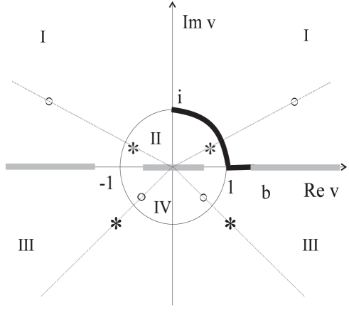
Figure 1: Uniformization plane for the $\pi\pi$-scattering amplitude.

In Fig.1, the plane of the uniformizing variable $v$ for the $\pi\pi$-scattering amplitude is depicted. The Roman numerals(I,…, IV) denote the images of the corresponding sheets of the Riemann surface; the thick line represents the physical region; the points i, 1 and $b=\sqrt{(m_{K}+m_{\pi})/(m_{K}-m_{\pi})}$ correspond to the $\pi\pi,K\overline{K}$ thresholds and $s=\infty$, respectively; the shaded intervals $(-\infty,-b],~{}[-b^{-1},b^{-1}],~{}[b,\infty)$ are the images of the corresponding edges of the left-hand cut. The depicted positions of poles ($*$) and of zeros ($\circ$) give the representation of the type (a) resonance in $S_{11}$.

On $v$-plane the Le Couteur-Newton relations are [9, 12]

$$S_{11}=\frac{d(-v^{-1})}{d(v)},\quad S_{22}=\frac{d(v^{-1})}{d(v)},\quad S_{11}S_{22}-S_{12}^{2}=\frac{d(-v)}{d(v)}.$$ (3)

Then, the condition of the real analyticity implies $~{}d(-v^{*})=d^{*}(v)~{}$ for all $v$, and the unitarity needs the following relations to hold true for the physical $v$-values: $~{}|d(-v^{-1})|\leq|d(v)|$, $~{}~{}|d(v^{-1})|\leq|d(v)|,~{}$ $~{}|d(-v)|=|d(v)|$.

The $d$-function that on the $v$-plane already does not possess branch-points is taken as $~{}d=d_{B}d_{res}$, where  $d_{B}=B_{\pi}B_{K}$; $B_{\pi}$ contains the possible remaining $\pi\pi$-background contribution, related to exchanges in crossing channels; $B_{K}$ is that part of the $K\overline{K}$ background which does not contribute to the $\pi\pi$-scattering amplitude. The most considerable part of the background of the considered coupled processes related to the influence of the left-hand branch-point at $s=0$ is taken already in the uniformizing variable $v$ (2) into account. The function $d_{res}(v)$ represents the contribution of resonances, described by one of three types of the pole-zero clusters, i.e., except for the point $v=0$, it consists of the zero s of clusters:

$$d_{res}=v^{-M}\prod_{n=1}^{M}(1-v_{n}^{*}v)(1+v_{n}v),$$ (4)

where $M$ is the number of pairs of the conjugate zeros.

3 Analysis of experimental data

We analyze simultaneously the available experimental data on the $\pi\pi$-scattering [15] and the process $\pi\pi\to K\overline{K}$ [16] in the channel with $I^{G}J^{PC}=0^{+}0^{++}$. As data, we use the results of phase analyses which are given for phase shifts of the amplitudes ($\delta_{1}$ and $\delta_{12}$) and for moduli of the $S$-matrix elements $\eta_{1}$ (the elasticity parameter) and $\xi$:

$$S_{a}=\eta_{a}e^{2i\delta_{a}}~{}~{}~{}~{}(a=1,2),\qquad S_{12}=i\xi e^{i\delta_{12}}.$$ (5)

(”1” denotes the $\pi\pi$ channel, ”2” – $K\overline{K}$). The 2-channel unitarity condition gives   $\eta_{1}=\eta_{2}=\eta,~{}~{}\xi=(1-\eta^{2})^{1/2},~{}~{}\delta_{12}=\delta_{1}+\delta_{2}$.
We have taken the data on the $\pi\pi$ scattering from the threshold up to 1.89 GeV. Then, comparing experimental data for $\xi$ with calculated values using experimental points for $\eta$, one can see that the 2-channel unitarity takes place to about 1.4 GeV.

To obtain the satisfactory description of the $s$-wave $\pi\pi$ scattering from the threshold to 1.89 GeV, we have taken $B_{\pi}=1$, and three multichannel resonances turned out to be sufficient: the two ones of the type (a) ($f_{0}(665)$ and $f_{0}(980)$) and $f_{0}(1500)$ of the type (c). Therefore, in eq.(4) $M=8$ and the following zero positions on the $v$-plane, corresponding to these resonances have been established in this situation with the parameterless description of the background:

$${\rm for}~{}~{}f_{0}(665):~{}~{} v_{1}=1.36964+0.208632i,\qquad~{}~{}v_{2}=0.921962-0.25348i,$$

$${\rm for}~{}~{}f_{0}(980):~{} v_{3}=1.04834+0.0478652i,\qquad~{}v_{4}=0.858452-0.0925771i,$$

$${\rm for}~{}~{}f_{0}(1500): v_{5}=1.2587+0.0398893i,\qquad~{}~{}~{}v_{6}=1.2323-0.0323298i,$$

$$v_{7}=0.809818-0.019354i,\qquad~{}v_{8}=0.793914-0.0266319i.$$

For $\delta_{1}$ and $\eta$, 113 and 50 experimental points [15], respectively, are used; when rejecting the points at energies 0.61, 0.65, and 0.73 GeV for $\delta_{1}$ and at 0.99, 1.65, and 1.85 GeV for $\eta$, which give an anomalously large contribution to $\chi^{2}$, we obtain for $\chi^{2}/\mbox{ndf}$ the values 2.7 and 0.72, respectively; the total $\chi^{2}/\mbox{ndf}$ in the case of the $\pi\pi$ scattering is 1.96. The corresponding curves (solid) demonstrating the quality of these fits are shown in Figs. 2 and 3.

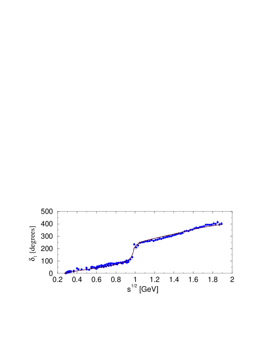
Figure 2: The energy dependence of the phase shift $\delta_{1}$ of the $\pi\pi$ scattering amplitude obtained on the basis of a simultaneous analysis of the experimental data on the coupled processes $\pi\pi\to\pi\pi,K\overline{K}$ in the channel with $I^{G}J^{PC}=0^{+}0^{++}$ for both versions – without and with the $f_{0}(1370)$ state: the solid curve corresponds to version 1; the dot-dashed one, version 2 (for $\delta_{1}$ the both curves practically coincide). The data on the $\pi\pi$ scattering are taken from Refs. [15].

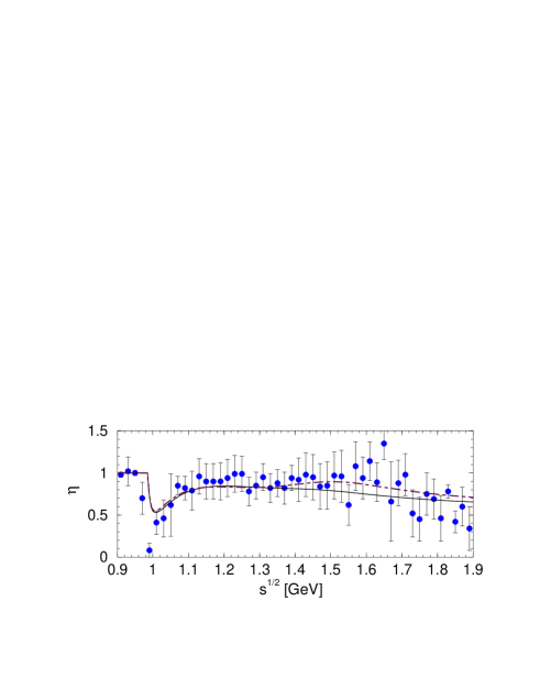
Figure 3: The same as in Fig. 2 but for the elasticity parameter $\eta$.

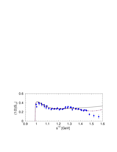
Figure 4: The energy dependences of the ($|S_{12}|$) for both soluitons: the solid curve corresponds to solution (1); the dot-dashed one, solution (2). The data on the process $\pi\pi\to K\overline{K}$ are taken from Refs. [16].

With the presented picture, the satisfactory description for the modulus ($\xi$) of the $\pi\pi\to K\overline{K}$ matrix element is given from the threshold to $\sim$ 1.4 GeV (Fig.4, the solid curve). Here 35 experimental points [16] are used; $\chi^{2}/\mbox{ndf}\approx 1.11$ when eliminating the points at energies 1.002, 1.265, and 1.287 GeV (with especially large contribution to $\chi^{2}$). However, for the phase shift $\delta_{12}(s)$, slightly excessive curve is obtained. Therefore, keeping the parameterless description of the $\pi\pi$ background, one must take into account the part of the $K\overline{K}$ background that does not contribute to the $\pi\pi$-scattering amplitude. Note that the variable $v$ is uniformizing for the $\pi\pi$-scattering amplitude, i.e., on the $v$-plane, $S_{11}$ has no cuts, however, the amplitudes of the $K\overline{K}$ scattering and $\pi\pi\to K\overline{K}$ process do have the cuts on the $v$-plane, which arise from the left-hand cut on the $s$-plane, starting at the point $s=4(m_{K}^{2}-m_{\pi}^{2})$. This left-hand cut will be neglected in the Riemann-surface structure, and the contribution on the cut will be taken into account in the $K\overline{K}$ background as a pole on the real $s$-axis on the physical sheet in the sub-$K\overline{K}$-threshold region. On the $v$-plane, this pole gives two poles on the unit circle in the upper half-plane, symmetric to each other with respect to the imaginary axis, and two zeros, symmetric to the poles with respect to the real axis, i.e., at describing the process $\pi\pi\to K\overline{K}$, one additional parameter is introduced, say, a position $p$ of the zero on the unit circle. Therefore, for $B_{K}$ we take the form

$$B_{K}=v^{-4}(1-pv)^{4}(1+p^{*}v)^{4}.$$ (6)

The fourth power in (6) is stipulated by the following. First, a pole on the real $s$-axis on the physical sheet in $S_{22}$ is accompanied by a pole in sheet II at at the same $s$-value (as it is seen from eqs. (2)); on the $v$-plane, this implies the pole of second order. Second, for the $s$-channel process $\pi\pi\to K\overline{K}$, the crossing $u$- and $t$-channels are the $\pi-K$ and $\overline{\pi}-K$ scattering (exchanges in these channels give contributions on the left-hand cut). This results in the additional doubling of the multiplicity of the indicated pole on the $v$-plane. The expression (6) does not contribute to $S_{11}$, i.e., the parameterless description of the $\pi\pi$ background is kept. A satisfactory description of the phase shift $\delta_{12}(\sqrt{s})$ (Fig.5) is obtained to $\sim$ 1.52 GeV with the value of $p=0.948201+0.31767i$ (this corresponds to the pole position on the $s$-plane at $s=0.434{\rm GeV}^{2}$).

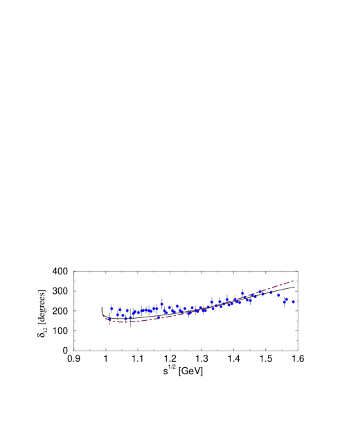
Figure 5: The same as in Fig. 4 but for the phase shift ($\delta_{12}$).

Here 59 experimental points [16] are considered; $\chi^{2}/\mbox{ndf}\approx 3.05$ when eliminating the points at energies 1.117, 1.247, and 1.27 GeV (with especially large contribution to $\chi^{2}$). The total $\chi^{2}/\mbox{ndf}$ for four analyzed quantities to describe the processes $\pi\pi\to\pi\pi,K\overline{K}$ is 2.12; the number of adjusted parameters is 17.

In Table 1, the obtained poles on the corresponding sheets of the Riemann surface are shown on the complex energy plane ($\sqrt{s_{r}}=={\rm E}_{r}-i\Gamma_{r}$). Since, for wide resonances, values of masses and widths are very model-dependent, it is reasonable to report characteristics of pole clusters which must be rather stable for various models.

Table 1: Pole clusters for obtained resonances in solution (1).

	$f_{0}(665)$		$f_{0}(980)$		$f_{0}(1500)$
Sheet	E, MeV	$\Gamma$, MeV	E, MeV	$\Gamma$, MeV	E, MeV	$\Gamma$, MeV
II	610$\pm$14	620$\pm$26	988$\pm$5	27$\pm$8	1530$\pm$25	390$\pm$30
III	720$\pm$15	55$\pm$9	984$\pm$16	210$\pm$22	1430$\pm$35	200$\pm$30
					1510$\pm$22	400$\pm$34
IV					1410$\pm$24	210$\pm$38

Now we calculate the coupling constants of the obtained states with the $\pi\pi$ and $K\overline{K}$ systems through the residues of amplitudes at the pole on sheet II, expressing the $T$-matrix via the $S$-matrix as $~{}S_{ii}=1+2i\rho_{i}T_{ii}$, $~{}S_{12}=2i\sqrt{\rho_{1}\rho_{2}}T_{12}$, where $\rho_{i}=\sqrt{(s-4m_{i}^{2})/s}$, and taking the resonance part of the amplitude in the form $~{}T_{ij}^{res}=\sum_{r}g_{ir}g_{rj}D_{r}^{-1}(s),$ where $D_{r}(s)$ is an inverse propagator ($D_{r}(s)\propto s-s_{r}$). The obtained values of the coupling constants are given in Table 2 (we denote the coupling constants with the $\pi\pi$ and $K\overline{K}$ systems through $g_{1}$ and $g_{2}$, respectively).

Table 2: Coupling constants of the observed states with the $\pi\pi$ ($g_{1}$) and $K\overline{K}$ ($g_{2}$) systems in solution (1).

	$f_{0}(665)$	$f_{0}(980)$	$f_{0}(1500)$
$g_{1}$, GeV	$0.7477\pm 0.095$	$0.1615\pm 0.03$	$0.899\pm 0.093$
$g_{2}$, GeV	$0.834\pm 0.1$	$0.438\pm 0.028$

In this 2-channel approach, there is no point in calculating the coupling constant of the $f_{0}(1500)$ state with the $K\overline{K}$ system, because the 2-channel unitarity is valid only to 1.4 GeV, and, above this energy, there is a considerable disagreement between the calculated amplitude modulus $S_{12}$ and experimental data.

We see that a minimum scenario of the simultaneous description of the processes $\pi\pi\to\pi\pi,K\overline{K}$ does not require the ${f_{0}}(1370)$ resonance. Therefore, if this meson exists, it must be relatively more weakly coupled to the $\pi\pi$ channel than to the $K\overline{K}$ one, i.e., it should be described by the pole cluster of type (b) (this would testify to the dominant $s{\bar{s}}$ component in this state). To confirm quantitatively this qualitative conclusion [17, 18] that is distinct from the one of other works [2], we consider the 2nd solution including the ${f_{0}}(1370)$ of type (b) in addition to three above-observed resonances. In the figures, this solution is represented by the dot-dashed curves. The description of the $\pi\pi$ scattering from the threshold up to 1.89 GeV is practically the same as without the $f_{0}(1370)$: $\chi^{2}/\mbox{ndf}$ for two quantities $\delta_{1}$ and $\eta$ is 2.01. The description of experimental data is improved a little for $|S_{12}|$ which is described now up to $\sim$ 1.46 GeV. For this quantity, we consider now 41 experimental points [16]; $\chi^{2}/\mbox{ndf}\approx 0.92$. However, on the whole, the description is even worse as compared with the 1st solution: the total $\chi^{2}/\mbox{ndf}\approx 2.93$ for four analyzed quantities describing the processes $\pi\pi\to\pi\pi,K\overline{K}$ (cf. 2.12 for the 1st case). The number of adjusted parameters is 21, where they all are positions of the poles describing resonances except a single one related to the $K\overline{K}$ background which is $p=0.976745+0.214405i$ (this corresponds to the pole on the $s$-plane at $s=0.622{\rm GeV}^{2}$). Let us indicate the obtained zero positions on the $v$-plane, corresponding to considered resonances in version 2:

$${\rm for}~{}~{}f_{0}(665):~{}~{} v_{1}=1.36783+0.212659i,\qquad~{}~{}v_{2}=0.921962-0.25348i,$$

$${\rm for}~{}~{}f_{0}(980):~{} v_{3}=1.04462+0.0479703i,\qquad~{}v_{4}=0.858452-0.0925771i,$$

$${\rm for}~{}~{}f_{0}(1370):~{} v_{5}=1.22783-0.0483842i,\qquad~{}v_{6}=0.802595-0.0379537i,$$

$${\rm for}~{}~{}f_{0}(1500): v_{7}=1.2587+0.0398893i,\qquad~{}~{}~{}v_{8}=1.24837-0.0358916i,$$

$$v_{9}=0.804333-0.0179899i,\qquad~{}v_{1}0=0.795579-0.0253985i.$$

In Table 3, the obtained poles on the corresponding sheets of the Riemann surface are shown on the complex energy plane ($\sqrt{s_{r}}={\rm E}_{r}-i\Gamma_{r}$).

Table 3: Pole clusters for obtained resonances in solution (2).

	$f_{0}(665)$		$f_{0}(980)$		$f_{0}(1370)$		$f_{0}(1500)$
Sheet	E, MeV	$\Gamma$, MeV	E, MeV	$\Gamma$, MeV	E, MeV	$\Gamma$, MeV	E, MeV	$\Gamma$, MeV
II	610$\pm$14	610$\pm$26	986$\pm$5	25$\pm$8			1530$\pm$22	390$\pm$28
III	720$\pm$15	55$\pm$9	984$\pm$16	210$\pm$25	1340$\pm$21	380$\pm$25	1490$\pm$30	220$\pm$25
							1510$\pm$22	370$\pm$30
IV					1330$\pm$18	270$\pm$20	1490$\pm$20	300$\pm$35

When calculating the coupling constants, we must take, for the ${f_{0}}(1370)$ state, the residues of amplitudes at the pole on sheet IV. In Table 4, the obtained values of coupling constants are shown. We see that the ${f_{0}}(980)$ and especially the ${f_{0}}(1370)$ are coupled essentially more strongly to the $K\overline{K}$ system than to the $\pi\pi$ one. This tells about the dominant $s{\bar{s}}$ component in the ${f_{0}}(980)$ state and especially in the ${f_{0}}(1370)$ one.

Table 4: Coupling constants of the observed states with the $\pi\pi$ ($g_{1}$) and $K\overline{K}$ ($g_{2}$) systems in solution (2).

	$f_{0}(665)$	$f_{0}(980)$	$f_{0}(1370)$	$f_{0}(1500)$
$g_{1}$, GeV	$0.724\pm 0.095$	$0.153\pm 0.03$	$0.11\pm 0.03~{}$	$0.866\pm 0.09$
$g_{2}$, GeV	$0.582\pm 0.1$	$0.521\pm 0.028$	$0.91\pm 0.04$

Let us indicate also scattering lengths calculated for both solutions. For the $K\overline{K}$ scattering, we obtain

$$a_{0}^{0}(K\overline{K})=-1.188\pm 0.13+(0.648\pm 0.09)i,~{}[m_{\pi^{+}}^{-1}];~{}~{}~{}({\rm solution(1)}),$$

$$a_{0}^{0}(K\overline{K})=-1.497\pm 0.12+(0.639\pm 0.08)i,~{}[m_{\pi^{+}}^{-1}];~{}~{}~{}({\rm solution(2)}).$$

The presence of the imaginary part in $a_{0}^{0}(K\overline{K})$ reflects the fact that, already at the threshold of the $K\overline{K}$ scattering, other channels ($2\pi,4\pi$ etc.) are opened. We see that the real part of $K\overline{K}$ scattering length is very sensitive to the existence of the ${f_{0}}(1370)$ state.

In Table 5, we compare our results for the $\pi\pi$ scattering length $a_{0}^{0}$ obtained for both solutions with results of other works both theoretical and experimental ones.

Table 5: Comparison of results of various works for the $\pi\pi$ scattering length $a_{0}^{0}$.

$a_{0}^{0},~{}m_{\pi^{+}}^{-1}$	References	Remarks
$0.27\pm 0.06$ (1)	our paper	model-independent approach
$0.266$        (2)
$0.26\pm 0.05$	L. Rosselet et al.[15]	analysis of the decay $K\to\pi\pi e\nu$
		using Roy’s model
$0.24\pm 0.09$	A.A. Bel’kov et al.[15]	analysis of $\pi^{-}p\to\pi^{+}\pi^{-}n$
		using the effective range formula
$0.23$	S. Ishida et al.[6]	modified analysis of $\pi\pi$ scattering
		using Breit-Wigner forms
$0.16$	S. Weinberg [19]	current algebra (nonlinear $\sigma$-model)
$0.20$	J. Gasser, H. Leutwyler [20]	one-loop corrections, nonlinear
		realization of chiral symmetry
$0.217$	J. Bijnens at al.[21]	two-loop corrections, nonlinear
		realization of chiral symmetry
$0.26$	M.K. Volkov [22]	linear realization of chiral symmetry
$0.28$	A.N. Ivanov, N.I. Troitskaya [23]	a variant of chiral theory with
		linear realization of chiral symmetry

We see that our results correspond to the linear realization of chiral symmetry.

We have here presented model-independent results: the pole positions, coupling constants, and scattering lengths. Masses and widths of these states that should be calculated from the obtained pole positions and coupling constants are highly dependent on the used model. Let us demonstrate this.

If the state $f_{0}(665)$ is the $\sigma$-meson, then from the known relation

$$g_{\sigma\pi\pi}=\frac{m_{\sigma}^{2}-m_{\pi}^{2}}{\sqrt{2}f_{\pi^{0}}}$$

(here $f_{\pi^{0}}$ is the constant of the weak decay of the $\pi^{0}$: $f_{\pi^{0}}=93.1$ MeV) we obtain  $m_{\sigma}\approx 342$ MeV. That small value of the $\sigma$-mass can be explained in part by the mixing with the $f_{0}(980)$ state [24]. If we take the resonance part of the amplitude as

$$T^{res}=\frac{\sqrt{s}\Gamma}{m_{\sigma}^{2}-s-i\sqrt{s}\Gamma,}$$

we obtain $m_{\sigma}\approx 850$ MeV and $\Gamma\approx 1240$ MeV.

4 Conclusions

In the model-independent approach consisting in the immediate application to the analysis of experimental data of first principles (analyticity-causality and unitarity), a simultaneous description of the isoscalar $s$-wave channel of the processes $\pi\pi\to\pi\pi,K\overline{K}$ from the thresholds to the energy values, where the 2-channel unitarity is valid, is obtained with three states ($f_{0}(665),f_{0}(980)$ and $f_{0}(1500)$) being sufficient. A parameterless description of the $\pi\pi$ background is given by allowance for the left-hand branch-point in the proper uniformizing variable. It is shown that the large $\pi\pi$-background, usually obtained in various analyses, combines in reality the influence of the left-hand branch-point and the contribution of a wide resonance at $\sim$ 665 MeV. Thus, a model-independent confirmation of the state denoted in the PDG issues by $f_{0}(400-1200)$ [2] is obtained. This is the $\sigma$-meson required by majority of models for spontaneous breaking of chiral symmetry. Note also that a light $\sigma$-meson is needed, for example, for an explanation of $K\to\pi\pi$ transitions using a Dyson – Schwinger model [25]. We emphasize that we have given, in fact, the first real proof of the $\sigma$-meson existence, because our analysis is based only on the first principles (i.e.,it is dynamical-free) and on the mathematical fact that a local behaviour of analytic functions determined on the Riemann surface is governed by the nearest singularities on all sheets and makes no additional assumptions about the the $\pi\pi$ background. For these reasons, the obtained results are rather model-independent. A multichannel state is represented by one of the standard clusters (poles on the Riemann surface) which is a qualitative characteristic of a state and a sufficient condition of its existence. The pole cluster gives the main effect of a multichannel state. The cluster type must be defined by a state nature. The compactness of a cluster and smoothness of the background are criteria of the description being correct.

On the basis of the fact that all the adjusted parameters of describing the $\pi\pi$ scattering are positions of poles corresponding to resonances (because the parameterless description of the $\pi\pi$ background is achieved), we conclude that our model-independent approach is a valuable tool for studying the realization schemes of chiral symmetry. The existence of $f_{0}(665)$ and the obtained $\pi\pi$-scattering length ($a_{0}^{0}(\pi\pi)\approx 0.27~{}m_{\pi^{+}}^{-1}$) suggest the linear realization of chiral symmetry.

The discovery of the $f_{0}(665)$ state solves one important mystery of the scalar-meson family that is related to the Higgs boson of the hadronic sector. This is a result of principle, because the schemes of the nonlinear realization of the chiral symmetry have been considered which do without the Higgs mesons. One can think that a linear realization of the chiral symmetry (at least, for the lightest states and related phenomena) is valid. First, this is a simple and beautiful mechanism that works also in other fields of physics, for example, in superconductivity. Second, the effective Lagrangians obtained on the basis of this mechanism (the Nambu – Jona-Lasinio and other models) describe perfectly the ground states and related phenomena.

The analysis of the used experimental data tells that, if the ${f_{0}}(1370)$ resonance exists (soluiton (2)), it has the dominant $s{\bar{s}}$ component, because the ratio of its coupling constant with the $\pi\pi$ channel to the one with the $K\overline{K}$ channel is 0.12 (as to that assignment of the ${f_{0}}(1370)$ resonance, we agree, e.g., with the work [26]). A minimum scenario of the simultaneous description of the processes $\pi\pi\to\pi\pi,K\overline{K}$ does without the ${f_{0}}(1370)$ resonance. The $K\overline{K}$ scattering length is very sensitive to the existence of this state.

The $f_{0}(1500)$ state is represented by the pole cluster which corresponds to a glueball. This type of clusters reflects the flavour-singlet structure of the glueball wave function and is only a necessary condition of the glueball nature of the $f_{0}(1500)$ state.

We think that multichannel states are most adequately represented by clusters, i.e. by the pole positions on all corresponding sheets. The pole positions are rather stable characteristics for various models, whereas masses and widths are very model-dependent for wide resonances.

Finally, note that in the model-independent approach, there are many adjusted parameters (although, e.g. for the $\pi\pi$ scattering, they all are positions of poles describing resonances). The number of these parameters can be diminished by some dynamic assumptions, but this is another approach and of other value.

This work has been supported by the Grant Program of Plenipotentiary of Slovak Republic at JINR. Yu.S. and M.N. were supported in part by the Slovak Scientific Grant Agency, Grant VEGA No. 2/7175/20; and D.K., by Grant VEGA No. 2/5085/99.

References

- [1] D. Krupa, V.A. Meshcheryakov, Yu.S. Surovtsev, Nuovo Cim. A109, 281 (1996).
- [2] Review of Particle Physics, Europ. Phys. J. C15, 1 (2000).
- [3] Y. Nambu, G. Jona-Lasinio, Phys. Rev. 122, 345 (1961); M.K. Volkov, Ann. Phys. 157, 282 (1984); T. Hatsuda, T. Kunihiro, Phys. Rep. 247, 223 (1994); R. Delbourgo, M.D. Scadron, Mod. Phys. Lett. A10, 251 (1995).
- [4] B.S. Zou, D.V. Bugg, Phys. Rev. D50, 591 (1994).
- [5] M. Svec, Phys. Rev. D53, 2343 (1996).
- [6] S. Ishida et al., Progr. Theor. Phys. 95, 745 (1996); ibid., 98, 621 (1997).
- [7] N. Törnqvist, Phys. Rev. Lett. 76, 1575 (1996).
- [8] R. Kamiński, L. Leśniak, B. Loiseau, Eur. Phys. J. C9, 141 (1999).
- [9] D. Krupa, V.A. Meshcheryakov, Yu.S. Surovtsev, Yad. Fiz. 43, 231 (1986); Czech. J. Phys. B38, 1129 (1988).
- [10] D. Morgan, M.R. Pennington, Phys. Rev. D48, 1185 (1993).
- [11] K.J. Le Couteur, Proc. Roy. Soc. A256, 115 (1960); R.G. Newton, J. Math. Phys. 2, 188 (1961).
- [12] M. Kato, Ann. Phys. 31, 130 (1965).
- [13] J. Boháčik, H. Kühnelt, Phys. Rev. D21, 1342 (1980).
- [14] B.V. Bykovsky, V.A. Meshcheryakov, D.V. Meshcheryakov, Yad. Fiz. 53, 257 (1990).
- [15] B. Hyams et al., Nucl. Phys. B64, 134 (1973); ibid., 100, 205 (1975); A. Zylbersztejn et al., Phys. Lett. B38, 457 (1972); P. Sonderegger, P. Bonamy, Proc. 5th Intern. Conf. on Elementary Particles (Lund, 1969) paper 372; J.R. Bensinger et al., Phys. Lett. B36, 134 (1971); J.P. Baton et al., Phys. Lett. B33, 525, 528 (1970); P. Baillon et al., Phys. Lett. B38, 555 (1972); L. Rosselet et al., Phys. Rev. D15, 574 (1977); A.A. Kartamyshev et al., Pis’ma v Zh. Eksp. Teor. Fiz. 25, 68 (1977); A.A. Bel’kov et al., Pis’ma v Zh. Eksp. Teor. Fiz. 29, 652 (1979).
- [16] A.B. Wicklund et al., Phys. Rev. Lett. 45, 1469 (1980); D. Cohen et al., Phys. Rev. D22, 2595 (1980); A. Etkin et al., Phys. Rev. D25, 1786 (1982).
- [17] Yu.S. Surovtsev, D. Krupa, M.Nagy, Acta Physica Polonica B31, 2697 (2000).
- [18] Yu.S. Surovtsev, D. Krupa, M. Nagy. Phys. Rev., D63, 054024 (2001).
- [19] S. Weinberg, Phys. Rev. Lett. 17, 616 (1966); B.W. Lee, H.T. Nieh, Phys. Rev. 166, 1507 (1968).
- [20] J. Gasser, H. Leutwyler, Ann. Phys. 158, 142 (1984).
- [21] J. Bijnens et al., Phys. Lett. B374, 210 (1996).
- [22] M.K. Volkov, Phys. Elem. Part. Atom. Nuclei 17, part 3, 433 (1986).
- [23] A.N. Ivanov, N.I. Troitskaya, Nuovo Cim. A108, 555 (1995).
- [24] M.K. Volkov, V.L. Yudichev, M. Nagy, Nuovo Cim. A112, 225 (1999).
- [25] J.C.R. Bloch et al., Phys. Rev. C62, 025206 (2000).
- [26] L.S. Celenza, Huangsheng Wang, C.M. Shakin, Preprint of Brooklyn College of the City Univ. of New York, BCCNT: 00/041/289 (2000).