High energy behaviour of $\gamma\gamma\to f\bar{f}$ processes in SM and MSSM

Abstract

We compute the leading logarithms electroweak contributions to $\gamma\gamma\to f\bar{f}$ processes in SM and MSSM. Several interesting properties are pointed out, such as the importance of the angular dependent terms, of the Yukawa terms, and especially of the $\tan^{2}\beta$ dependence in the SUSY contributions. These properties are complementary to those found in $e^{+}e^{-}\to f\bar{f}$ . These radiative correction effects should be largely observable at future high energy $\gamma\gamma$ colliders. Polarized beams would bring interesting checks of the structure of the one loop corrections. We finally discuss the need for two-loop calculations and resummation.

I Introduction.

The projects of high energy and high luminosity $e^{+}e^{-}$ colliders [1, 2] have recently motivated the study of the high energy behaviour of the electroweak corrections to several $e^{+}e^{-}$ annihilation processes. Explicit computations of the linear and quadratic logarithmic contributions to various observables have shown remarkable properties which should be largely observable at these future machines and should provide deep tests of the different sectors (gauge, matter, scalar) of the Standard Model (SM) as well as of its Supersymmetric extensions, like the Minimal Supersymmetric Standard Model (MSSM) [3, 4]. In fact, since many years, it was known that, in certain circumstances, large logarithmic terms, in particular quadratic logarithms can appear[5, 6]. The general features of the asymptotic one loop electroweak corrections have been studied, a classification of the linear and quadratic logarithms have been established, some two loop effects have been computed and the possibility of resumming certain classes of contributions have been discussed [7, 8, 9, 10, 11].

On another hand, the possibility of realizing high energy and high luminosity $\gamma\gamma$ collisions at $e^{+}e^{-}$ colliders through the laser backscattering procedure is actively considered [12, 13]. One already knows that electroweak radiative corrections to $\gamma\gamma\to f\bar{f}$ processes, both in the SM[14] and in the MSSM[15] are sizeable enough to be observable owing to the large luminosities expected at these machines which should allow to reach an accuracy better than the percent level.

The purpose of the present paper is to report on a study of the high energy behaviour of the electroweak corrections to the process $\gamma\gamma\to f\bar{f}$ in SM and in MSSM, performed along the same lines as those taken for the aforementioned studies of the $e^{+}e^{-}\to f\bar{f}$ processes. We will show that the $\gamma\gamma\to f\bar{f}$ processes offer an independent way to check the general properties of the asymptotic logarithmic terms originating from the various sectors of the electroweak interactions, and we will give precise numerical illustrations in order to see how they can be experimentally tested. A great similarity with the properties of the $e^{+}e^{-}\to f\bar{f}$ processes will appear and will allow us to conclude that $\gamma\gamma\to f\bar{f}$ processes can equally well contribute to the tests of the SM at high energies and to the search for its possible modifications or extensions.

The contents of the paper is the following. In Section II we present the dynamical contents in SM and in MSSM and we proceed with the computation of the complete one-loop weak contributions in the asymptotic regime. QED and QCD corrections are left aside as they depend on the detection conditions and are usually included in specific Monte-Carlo programs [14]. After having checked that the set of self-energy, vertex and box diagrams which are retained in the high energy limit is gauge-independent and satisfies photon current conservation, we systematically work in the $\xi=1$ gauge. We check the convergence of the separate contributions of the various sectors (neutral gauge, charged gauge, Yukawa) of the Standard Model (SM) , as well as of the additional SUSY terms (gaugino, higgsino, additional Higgs bosons). We keep the single and the quadratic logarithmic contributions. We separate the angular independent corrections from the angular dependent ones. All these contributions are specified for the helicity amplitudes of the process $\gamma\gamma\to f\bar{f}$; they are explicitly given in analytical form in Appendix A and B. From these expressions it is then easy to compute the various parts of the fully polarized $\gamma\gamma$ cross section. This is what we present in Section III. We then compute the effects on the various $\gamma\gamma$ observables and we present and discuss the results in the SM and MSSM cases. With the expected luminosity of LC and CLIC these various contributions should be experimentally observable. We then discuss the physics implications of the results as well as the domain of validity of the one-loop computation and the need of a two loop computation or a resummation at very high energies. This output is summarized in the concluding Section IV.

II Dynamical 1-loop contents of $\gamma\gamma\to f\bar{f}$ at high energy

We found convenient to express all the results in terms of helicity amplitudes [16] $F_{\lambda,\lambda^{\prime},\tau,\tau^{\prime}}$, $\lambda,\lambda^{\prime},\tau,\tau^{\prime}$ being the helicities of the two photons and of the fermion, antifermion, respectively; it is then easy to get the expressions of the observables in polarized photon-photon collisions.

The Born term consists in 2 diagrams with fermion exchange in the $t$ and $u$ channels. It is $\gamma\gamma$ symmetric; its amplitude, in the high energy limit, is written in Appendix A. It only contributes to the $|\Delta\lambda|=2$ helicity amplitudes.

At one-loop, the list of diagrams (to be symmetrized by interchanging the two photons) which contribute to the logarithmic terms in the high energy limit is given in Fig.1a-c for the SM case. In the MSSM case, the additional SUSY diagrams can be found in Fig.2a-b . We have checked that these contributions are ($\xi-1$)-independent and that current conservation ($l^{\mu}J_{\mu}=0$) holds separately for each photon. In Fig.1a-c,2a-b we have not drawn the external (photon, fermion) self-energy diagrams which do not contribute to the logarithmic terms, although they must be taken into account in order to get cancelation of the divergences generated by the internal fermion self-energy and by the triangular diagrams; box diagrams are convergent.

The explicit expressions of the helicity amplitudes in the high energy limit are given, separately for each sector of the electroweak corrections, in an analytical form in Appendix A. They are obtained by deriving the complete expressions of the amplitudes in terms of Passarino-Veltman functions [17], and retaining only the asymptotic (logarithmic) parts of these functions (see Appendix B). In a second step we only retain the terms which contain linear ($\ln s$) and quadratic ($\ln^{2}s$) logarithms,that we call ”leading terms”, neglecting terms like $\ln(t/s)$, ….etc, that we call ”non leading terms”. During this procedure we have checked that the divergences and the fermion mass singularities cancel. We have also separated the coefficients of the leading logarithms which are $\theta$-independent from those which are $\theta$-dependent ($\theta$ is the c.m. scattering angle). We now discuss in turn these various terms.

Standard Model corrections

$\gamma$ and $Z$ sectors

A first set of corrections is given by the internal fermion self-energy, triangle and box diagrams of Fig.1a containing one $Z$ boson. The corresponding helicity amplitudes are given in eq.(A3) and (A4) (terms proportional to ${[g^{Z}_{Vf}-g^{Z}_{Af}(2\tau)]^{2}/4s^{2}_{W}c^{2}_{W}}$). One can check in eqs.(A5),(A6) that the leading terms of the $|\Delta\lambda|=2$ helicity amplitude combine in an angular independent factor proportional to $[\ln^{2}(s/M^{2}_{Z})-3\ln(s/M^{2}_{Z})]$ multiplying the Born amplitude, in agreement with the general rule obtained in Ref.[10, 11] and that the correction to the $|\Delta\lambda|=0$ amplitude vanishes.

A similar set of corrections would be provided by the U.V. photon sector (cutted at scale $M_{Z}$), just replacing the internal $Z$ by an internal $\gamma$ in all the diagrams of Fig.1a. The result is given in eq.(A3) and (A4) (terms with $Q^{2}_{f}$ instead of ${[g^{Z}_{Vf}-g^{Z}_{Af}(2\tau)]^{2}/4s^{2}_{W}c^{2}_{W}}$). The properties of this ”$\gamma$ sector” are exactly similar to those of the $Z$ one. In the following numerical discussions we shall omit it, taking the stand point that all photonic corrections (the U.V. ones, the I.R. ones, including soft photon emission) should be put altogether inside ”QED-type” of corrections which depend on the characteristics of the detectors and are generally treated separately by specific programs. This is obviously a matter of choice, which can easily be modified.

$W$ sector

The corresponding diagrams are listed in Fig.1b. In addition to those which are obtained just by replacing the $Z$ by the $W$, there now appears new triangle and box diagrams involving the three-boson $\gamma WW$ coupling. The resulting amplitudes are given in eqs.(A9),(A13). One sees that the leading terms eqs.(A15),(A16) are enriched by angular dependent and angular independent contributions arising from the $\gamma WW$ coupling, which appear in addition to the $[\ln^{2}(s/M^{2}_{Z})-3\ln(s/M^{2}_{Z})]$ correction of the $|\Delta\lambda|=2$ amplitude.

Higgs sector

In SM the Higgs sector consists in the set of diagrams of Fig.1c involving charged and neutral $\Phi^{\pm,0}$ Goldstone bosons as well as the physical $H$ Higgs boson, coupled to fermions through Yukawa terms proportional to $m_{f}/M_{W}$. This set of diagrams is relevant only for top and bottom quark production. The resulting amplitudes are given in eqs.(A20),(A22) and their leading parts in eqs.(A24),(A25). As expected from the general properties established in [10, 11], these leading corrections coming from field renormalization constants (that one can directly obtain by solely considering external self-energy contributions) are angular independent, linearly logarithmic and only affect the $|\Delta\lambda|=2$ (Born) amplitude.

c) SUSY additional contributions

In the case of the MSSM, one should add to the previous SM terms the following additional SUSY corrections. We have separated them in two parts; first, a ”non massive part” arising from the diagrams of Fig.2a, in which only the mass-independent parts of the chargino and neutralino couplings are considered (corresponding to the charged or neutral ”gaugino” components); secondly, a ”massive part” due to the mass-dependent terms of the chargino and neutralino couplings (corresponding to the charged or neutral ”higgsino” components) and also to the diagrams involving SUSY Higgs bosons (to this last contributions we have subtracted the contribution of the standard $H_{SM}$ diagrams in order to not make double counting of the physical Higgs sector). A general remark, which was already made in the case of $e^{+}e^{-}$ collisions, is that, in the asymptotic regime $s>>M^{2}$, the only dependence in the MSSM parameters which remains is the dependence in $\tan\beta$; all other parameters (except the global SUSY scale $M$ appearing in the logarithmic terms) have disappeared because of the unitarity properties of the mixing matrices appearing in the SUSY couplings, see the fourth paper of Ref.[3].

Non massive terms

The amplitudes resulting from the mass-independent part of the diagrams of Fig.2a are given in eqs.(A28),(A30), and their leading terms in eqs.(A31),(A32). For the same reason as in the case of the Higgs sector, the correction to the $|\Delta\lambda|=2$ amplitude is only linearly logarithmic, angular independent (they can also be obtained from the external self-energy contributions to the field renormalization constants), and the correction to the $|\Delta\lambda|=0$ amplitude vanishes asymptotically.

Massive terms

The amplitudes resulting from the mass-dependent part of the diagrams of Fig.2a and of Fig.2b are given in eqs.(A42),(A49), and their leading terms in eqs.(A51),(A52). They behave asymptotically in a way similar to the SM Yukawa terms, the correction to the $|\Delta\lambda|=2$ amplitude being also only linearly logarithmic and angular independent, and the correction to the $|\Delta\lambda|=0$ amplitude vanishing. However, an important fact is the appearance of a $\cot^{2}\beta$ dependence in the term proportional to $m^{2}_{t}/M^{2}_{W}$, and a $\tan^{2}\beta$ dependence in the term proportional to $m^{2}_{b}/M^{2}_{W}$ (which can be very important for large $\tan\beta$ values).
We also note that, in the MSSM, summing the SM and the additional SUSY contributions, the leading asymptotic massive terms combine in order to reproduce the massive SM contributions in which the $m^{2}_{t}/M^{2}_{W}$ terms have been multiplied by $2(1+\cot^{2}\beta)$ and the $m^{2}_{b}/M^{2}_{W}$ terms by $2(1+\tan^{2}\beta)$. This rule had already been obtained for the process $e^{+}e^{-}\to f\bar{f}$ in the fifth paper of Ref.[3].

Let us finish this section by making a comparison with the asymptotic properties observed in the case of $e^{+}e^{-}\to f\bar{f}$. In the ’t Hooft $\xi=1$ gauge, the contributions of the triangle and box contributions behave sometimes differently in the $e^{+}e^{-}$ and in the $\gamma\gamma$ cases. The single $Z$ and $W$ triangles get only linear logarithms in the $\gamma\gamma$ case, whereas they get linear and quadratic logarithms in $e^{+}e^{-}$; on the opposite the $WW$ triangle gets only a quadratic logarithm in $\gamma\gamma$ instead of the linear logarithm in $e^{+}e^{-}$. These differences are complemented by those of the box diagrams. In both $Z$ and $W$ sectors, the boxes produce linear and quadratic logarithms in $\gamma\gamma$, whereas in the $e^{+}e^{-}$ case the $ZZ$ box give only linear logarithms and the $WW$ box has both linear and quadratic logarithms. The Higgs and the SUSY sectors are very similar in the $\gamma\gamma$ and in the $e^{+}e^{-}$ cases. They only give linear logarithms, arising only from the triangle diagrams (and also from the internal fermion self-energy in the $\gamma\gamma$ case). The Higgs and SUSY box diagrams give no leading logarithms at all, in both $\gamma\gamma$ and $e^{+}e^{-}$ cases.

III Effects on the $\gamma\gamma\to f\bar{f}$ observables

Having obtained the explicit expressions of the helicity amplitudes, it is easy to compute the various elements of the polarized $\gamma\gamma$ cross section. The general expression is given in Appendix C. Due to Bose statistics, CP-invariance and real (asymptotic) amplitudes, the expression of the cross section including terms up to order $\alpha^{3}$ simplifies to:

$${d\sigma\over d\tau d\cos\theta} = {d\bar{L}_{\gamma\gamma}\over d\tau}\Bigg{\{}[1-\langle\xi_{2}\xi^{\prime}_{2}\rangle]{d\bar{\sigma}_{0}\over d\cos\theta}+[\langle\xi_{2}\rangle-\langle\xi^{\prime}_{2}\rangle]{d\bar{\sigma}_{2}\over d\cos\theta}$$ (4)

$$+[\langle\xi_{3}\rangle\cos 2\phi+\langle\xi_{3}^{\prime}\rangle\cos 2\phi^{\prime}]{d\bar{\sigma}_{3}\over d\cos\theta}$$

$$+[\langle\xi_{3}\xi_{3}^{\prime}\rangle\cos 2(\phi+\phi^{\prime})]{d\bar{\sigma}_{33}\over d\cos\theta}$$

$$+[\langle\xi_{2}\xi_{3}^{\prime}\rangle\cos 2\phi^{\prime}-\langle\xi_{3}\xi^{\prime}_{2}\rangle\cos 2\phi]{d\bar{\sigma}_{23}\over d\cos\theta}\Bigg{\}}\ \ ,$$

in which $d\bar{L}_{\gamma\gamma}/d\tau$ describes the photon-photon luminosity per unit $e^{-}e^{+}$ flux obtained by the laser backscattering method [12]; $\tau=s/s_{ee}$ where $s\equiv s_{\gamma\gamma}$. The Stokes parameters $(\xi_{2},\xi^{\prime}_{2})$, $(\xi_{3},~{}\xi^{\prime}_{3})$ and $(\phi,~{}\phi^{\prime})$ describe respectively the average helicities, transverse polarizations and azimuthal angles of the two backscattered photons, see ref.[19],

The Born amplitudes only feed the (Parity conserving) ${d\bar{\sigma}_{0}/d\cos\theta}$ and ${d\bar{\sigma}_{33}/d\cos\theta}$ terms. The one-loop effects feed all the above terms. Note the specific photon polarization dependences which can be used to test the structure of the one-loop electroweak corrections and the absence of unexpected effects. Taking into account the fact that

$${d\bar{\sigma}_{0}\over d\cos\theta},~{}~{}~{}{d\bar{\sigma}_{3}\over d\cos\theta},~{}~{}~{}{d\bar{\sigma}_{33}\over d\cos\theta}$$

are $\cos\theta$-symmetric and

$${d\bar{\sigma}_{2}\over d\cos\theta},~{}~{}~{}{d\bar{\sigma}_{23}\over d\cos\theta}$$

$\cos\theta$-antisymmetric, we construct the five ratios;

$$R_{0}=\int d\cos\theta~{}[{d\bar{\sigma}_{0}\over d\cos\theta}-{d\bar{\sigma}^{Born}_{0}\over d\cos\theta}]~{}/\int d\cos\theta~{}{d\bar{\sigma}^{Born}_{0}\over d\cos\theta}$$ (5)

$$R_{33}=\int d\cos\theta~{}[{d\bar{\sigma}_{33}\over d\cos\theta}-{d\bar{\sigma}^{Born}_{33}\over d\cos\theta}]~{}/\int d\cos\theta~{}{d\bar{\sigma}^{Born}_{0}\over d\cos\theta}$$ (6)

$$R_{2}=\int_{F-B}d\cos\theta~{}[{d\bar{\sigma}_{2}\over d\cos\theta}]~{}/\int d\cos\theta~{}{d\bar{\sigma}^{Born}_{0}\over d\cos\theta}$$ (7)

$$R_{3}=\int d\cos\theta~{}[{d\bar{\sigma}_{3}\over d\cos\theta}]~{}/\int d\cos\theta~{}{d\bar{\sigma}^{Born}_{0}\over d\cos\theta}$$ (8)

$$R_{23}=\int_{F-B}d\cos\theta~{}[{d\bar{\sigma}_{23}\over d\cos\theta}]~{}/\int d\cos\theta~{}{d\bar{\sigma}^{Born}_{0}\over d\cos\theta}$$ (9)

on which the electroweak effects are now illustrated and discussed.

One should first note, using the definitions of the various ”cross sections” given in Appendix C, that the last two ratios $R_{3}$ and $R_{23}$ only involve products of $|\Delta\lambda=0|$ with $|\Delta\lambda=2|$ amplitudes. As we have seen that, in the asymptotic regime (see for example the leading expressions written in Appendix A), the one-loop contributions to $|\Delta\lambda=0|$ amplitudes are much weaker than the one to $|\Delta\lambda=2|$ amplitudes, one expects that these two ratios are much weaker than the other three ones.

Angular distributions

The angular distribution of the unpolarized Born cross section ${d\sigma^{Born}_{0}/d\cos\theta}$ is (symmetrically) strongly peaked in the forward and backward directions, see Fig.3a-c at $3~{}TeV$. The electroweak corrections modify somewhat this distribution because their effect is larger in the central region, as shown in Fig.4a-c where we plot the angular dependence of the relative effect of the electroweak corrections, defined as

$$\Delta({d\sigma_{0}\over d\cos\theta})\equiv[{d\sigma_{0}\over d\cos\theta}-{d\sigma^{Born}_{0}\over d\cos\theta}]/{d\sigma^{Born}_{0}\over d\cos\theta}\ .$$ (10)

It will therefore be interesting to have the largest possible angular acceptance allowed by experimental detection and to cut the angular distribution into several bins. One could then check the relative increase of the weak corrections in the central region.

Note that the radiative correction effect is always negative, that the supersymmetric corrections always increase the magnitude of the effect, and in the case of $t\bar{t}$, $b\bar{b}$ that this effect strongly depends on $\tan\beta$.

We now study in more details the behaviour of these effects versus the energy, by considering the integrated cross sections. In the following illustrations we choose to integrate the angular distributions in the domain $30^{0}<\theta<150^{0}$.

Leading versus non leading terms

It is interesting to compare, as a function of the energy, the relative importance of the various logarithmic terms which have been presented in the previous Section II. We will do that by considering the ratio $R_{0}$ giving the relative electroweak effects on the unpolarized cross section, defined in eq.(5).

In Fig.5a,b for $l^{+}l^{-}$, Fig.6a,b,c for $t\bar{t}$, Fig.7a,b,c for $b\bar{b}$ we show, separately for the SM and the MSSM cases, the contribution of the sum of all logarithmic terms (collected in Appendix A and B), compared to the results obtained when dropping the non leading logarithmic terms (i.e. terms of the type $\ln^{2}(t/s)$,… etc) and also to the results obtained when dropping, in addition, the leading angular dependent terms (terms $ln(s/M^{2})$ multiplied by angular dependent logarithms).

One sees that the non leading logarithmic terms (which appear in the expressions of the box contributions given in Appendix B) behave roughly like an additional small constant contribution (of the order of one percent) whose relative importance as compared to the full electroweak correction, decreases with the energy; this is true for both the SM and the MSSM cases.

On the contrary, the leading angular dependent terms (which appear in the triangle diagrams involving the $\gamma WW$ three boson coupling) are more important (similar effects has been noticed in Ref.[11], in the case of the crossed channel $e^{+}e^{-}\to\gamma\gamma$) and increase with the energy. They cannot be omitted at all, and we will come back to their role in the final discussion. This comment applies to both the SM and the MSSM cases, as the SUSY additional contributions only consist in angular independent contributions.

We have checked that, around $1$ TeV, our asymptotic results agree with those obtained in Ref.[14] for the purely weak part of the SM corrections to light fermion pair production. In the $t\bar{t}$ case, the agreement at $1$ TeV is only qualitative, for both the SM case [14] and the MSSM case [15], as this energy is just marginally ”asymptotic” for top quarks and for supersymmetric contributions. Nevertheless the cancellation of the various MSSM parameters, except for the large $\tan\beta$ dependence that we emphasized, can already be seen at this energy in [15].

Importance of Yukawa terms

In Fig.6a,b,c for $t\bar{t}$, Fig.7a,b,c for $b\bar{b}$, we have also shown the effect of dropping the Yukawa terms (coming from the Higgs and the Higgsino sectors) proportional to $m^{2}_{t}/M^{2}_{W}$ and $m^{2}_{b}/M^{2}_{W}$. Comparing the curves for the SM case and the curves for the case with no Yukawa terms in Fig.6a for $t\bar{t}$, and Fig.7a for $b\bar{b}$, one sees that these terms are very important, especially in the $t\bar{t}$ case, where they contribute easily for half of the effect at CLIC energies. In the MSSM case, the comparison is made in Fig.6b and 7b for $\tan\beta=4$, and in Fig.6c and 7c for $\tan\beta=40$. The $\tan\beta$ dependence can be understood by looking at eq.(A51), in which one sees a $\cot^{2}\beta$ dependence associated to the term $(m^{2}_{t}/M^{2}_{W})$ and a $\tan^{2}\beta$ dependence associated to the $(m^{2}_{b}/M^{2}_{W})$, which becomes dominant at very large $\tan\beta$ values. These properties are rather similar to those observed in $\gamma\gamma\to f\bar{f}$ [18].

Polarized and unpolarized cross sections versus the energy

We finally illustrate the behaviour of the various terms of the polarized cross section, eq.(4), versus the energy, in the $l^{+}l^{-}$, $t\bar{t}$ and $b\bar{b}$ cases.

In Fig.8a,b,c and 9a,b,c we present the ratios $R_{0}$ and $R_{33}$ which show the relative departures from the Born prediction, see eq.(5),(6). The effects are in all cases of the order of several percents at LC energies and of the order of 10-20 percents at CLIC energies. In the MSSM case they are larger than in the SM case, especially for large $\tan\beta$ values.

In Fig.10a,b,c , 11a,b,c and 12a,b,c we present the ratios $R_{2}$, $R_{3}$ and $R_{23}$ defined in eqs.(7),(8),(9). There is no Born contribution to these terms. The effects in $R_{2}$ (circular photon polarization dependence) are comparable to those previously seen in $R_{0}$. This is because $R_{2}$ measures the Parity violating effects which are maximal in $W$ couplings. On the contrary, the effects are very small in $R_{3}$ (one photon transversally polarized) and $R_{23}$ (one photon transversally polarized, the other one being circularly polarized)) because these terms, as we have already mentioned after their definitions, are proportional to the interference of small $\Delta\lambda=0$ amplitudes (which have no leading $ln(s/M^{2})$ or $ln^{2}(s/M^{2})$ terms) with $\Delta\lambda=2$ ones. Very high energies are required in order for these observables to reach the observable percent level.

We can add a final remark concerning the cross section for $\gamma\gamma$ to hadrons, the analogue of the cross section for hadron production in $e^{+}e^{-}$ collisions $\sigma_{5}\equiv\sigma(e^{+}e^{-}\to u\bar{u}+c\bar{c}+d\bar{d}+s\bar{s}+b\bar{b})$. In $\gamma\gamma$ collisions, as we can see from Fig.3b,c , because of the factor $Q_{f}^{4}$ in the Born cross section, the rate is largely dominated the contribution of up-quarks ($u,c$), and the Yukawa contribution, appearing solely in the $b$ case, can be completely neglected. So the properties of the electroweak radiative corrections to $\sigma(\gamma\gamma\to hadrons)$ can be totally inferred from those of $\sigma(\gamma\gamma\to t\bar{t})$, ignoring the Yukawa contributions; see for example the curves corresponding to the case with no Yukawa terms in Fig.6ab.

IV Conclusions

We have studied the high energy behaviour of the one-loop weak corrections to the processes $\gamma\gamma\to f\bar{f}$, in SM and in MSSM.

In the asymptotic energy regime, we have classified and computed all correction terms coming in the ’t Hooft $\xi=1$ gauge, from fermion self-energies, triangle and box diagrams. We have checked that, in each weak sector, the set of diagrams contributes in a gauge-independent way to the linear and quadratic logarithmic contributions to the $\gamma\gamma\to f\bar{f}$ amplitudes. Explicit analytic expressions are given in Appendix A and B, and turn out to be rather simple, and reflecting in a remarkable way the theoretical properties of the SM charged gauge, neutral gauge and Higgs sectors and of the MSSM gaugino and Higgsino sectors. These results satisfy the known general properties of leading electroweak logarithms at one loop [7, 10, 11]. They also match with the complete one loop computations performed around 1 TeV in[14, 15].

We have shown that these effects should be well visible in $\gamma\gamma$ collisions at LC and CLIC, the large luminosities expected at these machines allowing to reach an accuracy better than the percent level. We have given the results for five observables defined in the case of polarized photon beams. Clearly, the behaviour of each observable should provide clean tests of the SM or the MSSM and allow to check the absence of unexpected new physics effect.

An important fact is the strong rise of the effect on the cross section, partly due to the angular independent factor ${\alpha/4\pi}[\ln^{2}(s/M^{2}_{W})-3\ln(s/M^{2}_{W})]$, but we have shown that there are also important angular dependent contributions. A clear difference also appear, in each $f=l,~{}t,~{}b$ case, between the SM and the MSSM corrections. The SUSY additional terms increase the magnitude of the weak corrections. For example at $3$ TeV, in $l^{+}l^{-}$ production, the correction is -12.7% in SM and -13.6% in MSSM. In the $t\bar{t}$ and $b\bar{b}$ cases, the Yukawa terms contribute for a large part of the effects, both in SM and in MSSM; in this last case an observable $\tan\beta$ dependence appear. At $3$ TeV, the weak effects to $t\bar{t}$ production are -23.1% in SM, -27.2% in MSSM($\tan\beta=4$), -28.6% in MSSM($\tan\beta=40$); and for $b\bar{b}$ production, they are -32.3% in SM, -34.8% in MSSM($\tan\beta=4$), -41.6% in MSSM($\tan\beta=40$). This $\tan\beta$ dependence could be used for a $\tan\beta$ measurement (see the corresponding discussion in $e^{+}e^{-}$ collisions in Ref.[18]).

These results are complementary to those observed in the process $e^{+}e^{-}\to f\bar{f}$. We have shown that the role of the self-energy, triangle and box diagrams are different in the two processes, but the qualitative aspect of the information that can be reached about the features of the electroweak corrections is rather similar. There are however quantitative differences when comparing the effects in $l^{+}l^{-}$, $b\bar{b}$ and $t\bar{t}$ production. This is essentially due to the fact that in $\gamma\gamma$ collisions the Born term, proportional to $Q^{4}_{f}$, is especially small in the $b\bar{b}$ case, so that the electroweak corrections are relatively larger. Also the effects of gauge, Yukawa, and SUSY contributions cumulate so that the corrections are larger than in the $e^{+}e^{-}\to f\bar{f}$ processes at the same energy.

As these first order effects already reach the 10 percent level around 1 TeV, and 30 percent around 3 TeV, one may naively expect that higher order terms easily reach the few percent level, observable at CLIC, raising the question of a possible two-loop computation. For the angular independent terms, general resummation techniques has been proposed [resum], which would partly solve the problem. However we have shown that there are important angular dependent terms for which no prescription has yet been obtained and may require an explicit two-loop computation.

At lower energies (the 0.5 to 1 TeV domain of LC), there is apparently no such problem. Although the effect in $\gamma\gamma\to b\bar{b}$ can reach 15 percent at 1 TeV, the weaker experimental accuracy in this channel, may still allow to stay at the one-loop level. However, as we have shown by comparing leading and non leading logarithmic terms, in this energy range, the logarithmic approximation is probably not sufficient. Constant terms (and possibly terms of order $M^{2}/s$) may not be negligible, especially if the SUSY scale is rather high and one may not be allowed to neglect the mass of the SUSY particles running inside the loops. This approximation also fails to reproduce the ”resonance” effects which appear around the thresholds for (sfermion or chargino) pair production[15]. In this ”low energy” regime, the full set of MSSM parameters enter the game (and not only $\tan\beta$ as in the asymptotic regime). We intend to perform a detailed comparison of the logarithmic approximation with the exact computation of the full one-loop contributions. It should allow to understand the role and to discuss the measurability, in the LC regime, of each of the various MSSM parameters.

A Asymptotic expressions of the helicity amplitudes at one-loop

We denote by $F_{\lambda,\lambda^{\prime},\tau,\tau^{\prime}}$ the helicity amplitudes of the process $\gamma\gamma\to f\bar{f}$, $\lambda,\lambda^{\prime},\tau,\tau^{\prime}$ being the helicities of the photons ($\pm 1$), and of the fermion and antifermion ($\pm{1/2}$) in the $\gamma\gamma$ center of mass. We denote by $e,l$, $e^{\prime},l^{\prime}$ the photon polarization vectors and 4-momenta and $p,p^{\prime}$ the fermion, antifermion 4-momenta; $q=p-l=l^{\prime}-p^{\prime}$, $q^{\prime}=p-l^{\prime}=l-p^{\prime}$; $\sqrt{s}$, $\theta$ are the energy and the scattering angle.

We work in the high energy limit $s=(l+l^{\prime})^{2}=(p+p^{\prime})^{2},~{}t=q^{2}=-~{}{s/2}(1-\cos\theta),~{}u=q^{\prime 2}=-~{}{s/2}(1+\cos\theta)>>M^{2}$ (avoiding the forward and backward domains), keeping only logarithmic terms involving $s$, $t$ or $u$. A general consequence of the high energy limit is the dominance of chirality conserving terms with $\tau^{\prime}=-\tau$ only.

a) Born term

At high energy, the invariant amplitude corresponding to the diagrams of Fig.1 is:

$${\cal R}^{Born}=-~{}e^{2}Q^{2}_{f}\bar{u}_{f}(p)[{e\!\!\!/\ q\!\!\!/\ e\!\!\!/\ ^{\prime}\over t}+{e\!\!\!/\ ^{\prime}q\!\!\!/\ ^{\prime}e\!\!\!/\ \over u}]v_{\bar{f}}(p^{\prime})$$ (A1)

$Q_{f}$ is the fermion charge in unit of $|e|$.

It leads to the helicity amplitudes

$$F^{Born}_{\lambda,-\lambda,\tau,-\tau}=-~{}8\pi\alpha Q^{2}_{f}[{\lambda+2\tau\cos\theta\over\sin\theta}]$$ (A2)

Note that, at high energy, due to Bose symmetry, the Born term only involves $\lambda^{\prime}=-\lambda$ (i.e. $|\Delta\lambda|=2$) amplitudes.

b) SM electroweak corrections

$\gamma$ and $Z$ sector

The sum of self-energy, triangle and Box diagrams of Fig.1a (to which external fermion self-energy diagrams are added) is convergent and gives the asymptotic contributions:

$$F_{\lambda,-\lambda,\tau,-\tau} = \alpha^{2}Q^{2}_{f}\{Q^{2}_{f}+{[g^{Z}_{Vf}-g^{Z}_{Af}(2\tau)]^{2}\over 4s^{2}_{W}c^{2}_{W}}\}\{~{}2~{}[{\lambda+(2\tau)\cos\theta\over\sin\theta}]~{}\ln{s\over M^{2}_{Z}}+B^{1}_{\lambda,-\lambda}(M^{2}_{Z})\}$$ (A3)

$$F_{\lambda,\lambda,\tau,-\tau} = \alpha^{2}Q^{2}_{f}\{Q^{2}_{f}+{[g^{Z}_{Vf}-g^{Z}_{Af}(2\tau)]^{2}\over 4s^{2}_{W}c^{2}_{W}}\}\{-8~{}[{(2\tau)\cos\theta\over\sin\theta}]~{}\ln{s\over M^{2}_{Z}}+B^{1}_{\lambda,\lambda}(M^{2}_{Z})\}$$ (A4)

The box quantities $B^{i}$ are defined in Appendix B, and $g^{Z}_{Vf}=I_{3f}(1-4s^{2}_{W}|Q_{f}|)$, $g^{Z}_{Af}=I_{3f}$.

leading terms

$$F^{l.t.}_{\lambda,-\lambda,\tau,-\tau} \to-F^{Born}_{\lambda,-\lambda,\tau,-\tau}({\alpha\over 4\pi})\{Q^{2}_{f}+{[g^{Z}_{Vf}-g^{Z}_{Af}(2\tau)]^{2}\over 4s^{2}_{W}c^{2}_{W}}\}(\ln^{2}{s\over M^{2}_{Z}}-3\ln{s\over M^{2}_{Z}})$$ (A5)

$$F^{l.t.}_{\lambda,\lambda,\tau,-\tau} \to 0$$ (A6)

$W$ sector

We now sum the contributions of the charged gauge sector, with the self-energy, triangle and box diagrams of Fig.1b. Note that in order to get a convergent result, one has to add the photon self-energy contribution; it cancels the divergent contribution which appears in the axial term of the corrected $\gamma ff$ vertex; whereas a remaining divergence in the vector term is absorbed by the charge renormalization.

$$F_{\lambda,-\lambda,\tau,-\tau} = {\alpha^{2}\over 4s^{2}_{W}}[1-(2\tau)]\{[{\lambda+(2\tau)\cos\theta\over\sin\theta}][2Q_{f}(Q_{f}-2(2I_{3f}))\ln{s\over M^{2}_{W}}$$ (A9)

$$+Q_{f}(2I_{3f})[(1+\cos\theta)\ln^{2}{t\over m^{2}_{W}}+(1-\cos\theta)\ln^{2}{u\over m^{2}_{W}}]+2\sin^{2}\theta~{}\ln{s\over M^{2}_{W}}]$$

$$+[Q_{f}-(2I_{3f})]^{2}B^{1}_{\lambda,-\lambda}(M^{2}_{W})+B^{2}_{\lambda,-\lambda}(M^{2}_{W})-[Q_{f}-(2I_{3f})](2I_{3f})B^{5}_{\lambda,-\lambda}(M^{2}_{W})\}$$

$$F_{\lambda,\lambda,\tau,-\tau} = {\alpha^{2}\over 4s^{2}_{W}}[1-(2\tau)]\{(2\tau)[-8Q_{f}(Q_{f}-(2I_{3f})){\cos\theta\over\sin\theta}\ln{s\over M^{2}_{W}}$$ (A13)

$$+Q_{f}(2I_{3f})\sin\theta[{(2-\cos\theta)\over 1-\cos\theta}\ln^{2}{t\over m^{2}_{W}}-{(2+\cos\theta)\over 1+\cos\theta}\ln^{2}{u\over m^{2}_{W}}]$$

$$-2\sin\theta\cos\theta)\ln{s\over M^{2}_{W}}]$$

$$+[Q_{f}-(2I_{3f})]^{2}B^{1}_{\lambda,\lambda}(M^{2}_{W})+B^{2}_{\lambda,\lambda}(M^{2}_{W})-[Q_{f}-(2I_{3f})](2I_{3f})B^{5}_{\lambda,\lambda}(M^{2}_{W})\}$$

leading terms

$$F^{l.t.}_{\lambda,-\lambda,\tau,-\tau} \to-F^{Born}_{\lambda,-\lambda,\tau,-\tau}({\alpha\over 32\pi s^{2}_{W}Q^{2}_{f}})[1-(2\tau)]\{2Q^{2}_{f}(\ln^{2}{s\over M^{2}_{W}}-3\ln{s\over M^{2}_{W}})+4Q_{f}(2I_{3f})\ln^{2}{s\over M^{2}_{W}}$$ (A15)

$$+4[\cos\theta\ln{1-\cos\theta\over 1+\cos\theta}+(2Q_{f}(2I_{3f})-1)\ln{\sin^{2}\theta\over 4}]\ln{s\over M^{2}_{W}}\}$$

$$F^{l.t.}_{\lambda,\lambda,\tau,-\tau} \to 0$$ (A16)

Note the appearance of angular dependent leading terms. This is the only sector where it happens (such terms were also found in Ref.[11] in the crossed channel $e^{+}e^{-}\to\gamma\gamma$ for left-handed electrons). See the discussion in Sections II and III.

Higgs sector

We now add the contributions of the diagrams of Fig.1c involving the Goldstone $\Phi$ and the physical Higgs $H_{SM}$. This concerns only the production of massive quarks $f=t,b$, as these contributions, arising from the Yukawa couplings, are proportional to $m^{2}_{f}/M^{2}_{W}$.

$$F_{\lambda,-\lambda,\tau,-\tau} = {\alpha^{2}\over 4s^{2}_{W}}\{Q^{2}_{f}[{\lambda+(2\tau)\cos\theta\over\sin\theta}].$$ (A20)

$$.\{[{m^{2}_{t}\over M^{2}_{W}}(1+(2\tau)(2I_{3f}))+{m^{2}_{b}\over M^{2}_{W}}(1-(2\tau)(2I_{3f}))]+2({m^{2}_{f}\over M^{2}_{W}})\}\ln{s\over M^{2}_{W}}$$

$$+[B^{4}_{\lambda,-\lambda}+(Q_{f}-(2I_{3f}))^{2}B^{3}_{\lambda,-\lambda}-(Q_{f}-(2I_{3f}))(2I_{3f})B^{6}_{\lambda,-\lambda}].$$

$$.[{m^{2}_{t}\over M^{2}_{W}}(1+(2\tau)(2I_{3f}))+{m^{2}_{b}\over M^{2}_{W}}(1-(2\tau)(2I_{3f}))]+2Q_{f}^{2}({m^{2}_{f}\over M^{2}_{W}})B^{3}_{\lambda,-\lambda}\}\$$

$$F_{\lambda,\lambda,\tau,-\tau} = {\alpha^{2}\over 4s^{2}_{W}}\{[B^{4}_{\lambda,\lambda}+(Q_{f}-(2I_{3f}))^{2}B^{3}_{\lambda,\lambda}-(Q_{f}-(2I_{3f}))(2I_{3f})B^{6}_{\lambda,\lambda}].$$ (A22)

$$.[{m^{2}_{t}\over M^{2}_{W}}(1+(2\tau)(2I_{3f}))+{m^{2}_{b}\over M^{2}_{W}}(1-(2\tau)(2I_{3f}))]+2Q_{f}^{2}({m^{2}_{f}\over M^{2}_{W}})B^{3}_{\lambda,\lambda}\}$$

leading terms

$$F^{l.t.}_{\lambda,-\lambda,\tau,-\tau} \to-F^{Born}_{\lambda,-\lambda,\tau,-\tau}({\alpha\over 32\pi s^{2}_{W}})\{[{m^{2}_{t}\over M^{2}_{W}}(3+(2\tau))+{m^{2}_{b}\over M^{2}_{W}}(1-(2\tau))]\delta_{tf}$$ (A24)

$$+[{m^{2}_{b}\over M^{2}_{W}}(3+(2\tau))+{m^{2}_{t}\over M^{2}_{W}}(1-(2\tau))]\delta_{bf}\}\ln{s\over M^{2}_{W}}$$

$$F^{l.t.}_{\lambda,\lambda,\tau,-\tau} \to 0$$ (A25)

Note that the box functions $B^{3,4,6}$ (and consequently, the full Higgs contribution to $F_{\lambda,\lambda,\tau,-\tau})$ do not contribute to the leading $\ln s$ or $\ln^{2}s$ terms; so no scale is mentioned in their notation (see Appendix B); the same property holds in the following supersymmetric contributions.

c) SUSY additional contributions

Non massive terms

By non massive terms we mean the contributions due to the diagrams involving gauge couplings of sfermions, charginos and neutralinos. They come from self-energy, triangle and Box diagrams in Fig.2a (and external fermion self-energy terms).

$$F_{\lambda,-\lambda,\tau,-\tau} = {\alpha^{2}\over 4s^{2}_{W}}\{[{\lambda+(2\tau)\cos\theta\over\sin\theta}][2Q^{2}_{f}({2C_{f}Q^{2}_{f}\over c^{2}_{W}}+1-(2\tau))]\ln{s\over M^{2}}$$ (A28)

$$+[1-(2\tau)][2B^{3}_{\lambda,-\lambda}-2(Q_{f}-(2I_{3f}))(2I_{3f})B^{6}_{\lambda,-\lambda}+D_{f}B^{4}_{\lambda,-\lambda}]$$

$$+[1+(2\tau)]E_{f}B^{4}_{\lambda,-\lambda}\}$$

$$F_{\lambda,\lambda,\tau,-\tau} = {\alpha^{2}\over 4s^{2}_{W}}\{[1-(2\tau)][2B^{3}_{\lambda,\lambda}-2(Q_{f}-(2I_{3f}))(2I_{3f})B^{6}_{\lambda,\lambda}+D_{f}B^{4}_{\lambda,\lambda}]$$ (A30)

$$+[1+(2\tau)]E_{f}B^{4}_{\lambda,\lambda}\}$$

where

$$C_{l}={1\over 4}(1-(2\tau))+s^{2}_{W}(1+(2\tau)),~{}~{}~{}D_{l}={1\over c^{2}_{W}},~{}~{}~{}E_{l}={4s^{2}_{W}\over c^{2}_{W}}\ ,$$

$$C_{t}={9-8s^{2}_{W}\over 36}(1-(2\tau))+{4s^{2}_{W}\over 9}(1+(2\tau)),~{}~{}~{}D_{t}={2\over 9}+{4(9-8s^{2}_{W})\over 81c^{2}_{W}},~{}~{}~{}E_{t}={64s^{2}_{W}\over 81c^{2}_{W}}\ ,$$

$$C_{b}={9-8s^{2}_{W}\over 36}(1-(2\tau))+{s^{2}_{W}\over 9}(1+(2\tau)),~{}~{}~{}D_{b}={8\over 9}+{(9-8s^{2}_{W})\over 81c^{2}_{W}},~{}~{}~{}E_{b}={4s^{2}_{W}\over 81c^{2}_{W}}\ .$$

leading terms

$$F^{l.t.}_{\lambda,-\lambda,\tau,-\tau} \to-F^{Born}_{\lambda,-\lambda,\tau,-\tau}({\alpha\over 16\pi s^{2}_{W}})[({2C_{f}Q^{2}_{f}\over c^{2}_{W}}+1-(2\tau))]\ln{s\over M^{2}}$$ (A31)

$$F_{\lambda,\lambda,\tau,-\tau} \to 0$$ (A32)

$M$ is a common SUSY scale introduced for convenience (that will be fixed to $0.5~{}TeV$ in the illustrations). Note that a change of value of $M$ amounts to the introduction of additional (neglected) constant terms, as the SUSY contributions only appear with $\ln(s/M^{2})$ and never with quadratic logarithmic terms.
Note in addition that the SUSY contribution to $F_{\lambda,\lambda,\tau,-\tau}$ has also no leading $\ln s$ or $\ln^{2}s$ term.

Massive terms

These terms arise from the Yukawa couplings of the Higgsino component of the charginos and neutralinos interacting with sfermions, as well as from the physical SUSY Higgs contributions (from which we subtract the SM Higgs contribution in order to not make double counting of the Higgs sector contribution). From self-energy, triangle and box diagrams of Fig.2a,b (and external fermion self-energy terms) one gets:

$$F_{\lambda,-\lambda,\tau,-\tau} = {\alpha^{2}\over 4s^{2}_{W}}\{Q^{2}_{f}[{\lambda+(2\tau)\cos\theta\over\sin\theta}].$$ (A42)

$$\{.[{m^{2}_{t}\over M^{2}_{W}}(1+(2\tau)(2I_{3f}))(1+2\cot^{2}\beta)+{m^{2}_{b}\over M^{2}_{W}}(1-(2\tau)(2I_{3f}))(1+2\tan^{2}\beta)]$$

$$+2({m^{2}_{f}\over M^{2}_{W}})[(1+2\cot^{2}\beta)\delta_{tf}+(1+2\tan^{2}\beta)\delta_{bf}]\}\ln{s\over M^{2}}$$

$$+(B^{4}_{\lambda,-\lambda}+(Q_{f}-(2I_{3f}))^{2}B^{3}_{\lambda,-\lambda})[{m^{2}_{t}\over M^{2}_{W}}(1+(2\tau)(2I_{3f}))\cot^{2}\beta$$

$$~{}~{}~{}~{}~{}~{}~{}~{}~{}~{}~{}~{}~{}~{}~{}~{}~{}~{}~{}~{}~{}~{}~{}~{}~{}~{}~{}~{}~{}~{}~{}~{}~{}~{}~{}~{}~{}~{}~{}~{}~{}~{}~{}~{}~{}~{}~{}+{m^{2}_{b}\over M^{2}_{W}}(1-(2\tau)(2I_{3f}))\tan^{2}\beta]$$

$$+(B^{3}_{\lambda,-\lambda}+(Q_{f}-(2I_{3f}))^{2}B^{4}_{\lambda,-\lambda})[{m^{2}_{t}\over M^{2}_{W}}(1+(2\tau)(2I_{3f}))(1+\cot^{2}\beta)$$

$$~{}~{}~{}~{}~{}~{}~{}~{}~{}~{}~{}~{}~{}~{}~{}~{}~{}~{}~{}~{}~{}~{}~{}~{}~{}~{}~{}~{}~{}~{}~{}~{}~{}~{}~{}~{}~{}~{}~{}~{}~{}~{}~{}~{}~{}~{}~{}+{m^{2}_{b}\over M^{2}_{W}}(1-(2\tau)(2I_{3f}))(1+\tan^{2}\beta)]$$

$$-(Q_{f}-(2I_{3f}))(2I_{3f})B^{6}_{\lambda,-\lambda}.[{m^{2}_{t}\over M^{2}_{W}}(1+(2\tau)(2I_{3f}))(1+2\cot^{2}\beta)$$

$$~{}~{}~{}~{}~{}~{}~{}~{}~{}~{}~{}~{}~{}~{}~{}~{}~{}~{}~{}~{}~{}~{}~{}~{}~{}~{}~{}~{}~{}~{}~{}~{}~{}~{}~{}~{}~{}~{}~{}~{}~{}~{}~{}~{}~{}~{}~{}+{m^{2}_{b}\over M^{2}_{W}}(1-(2\tau)(2I_{3f}))(1+2\tan^{2}\beta)]$$

$$+2Q^{2}_{f}{m^{2}_{f}\over M^{2}_{W}}(B^{3}_{\lambda,-\lambda}[\cot^{2}\beta\delta_{tf}+\tan^{2}\beta\delta_{bf}]+B^{4}_{\lambda,-\lambda}[(1+\cot^{2}\beta)\delta_{tf}+(1+\tan^{2}\beta)\delta_{bf}])\}$$

$$F_{\lambda,\lambda,\tau,-\tau} = {\alpha^{2}\over 4s^{2}_{W}}\{(B^{4}_{\lambda,\lambda}+(Q_{f}-(2I_{3f}))^{2}B^{3}_{\lambda,\lambda})[{m^{2}_{t}\over M^{2}_{W}}(1+(2\tau)(2I_{3f}))\cot^{2}\beta$$ (A49)

$$~{}~{}~{}~{}~{}~{}~{}~{}~{}~{}~{}~{}~{}~{}~{}~{}~{}~{}~{}~{}~{}~{}~{}~{}~{}~{}~{}~{}~{}~{}~{}~{}~{}~{}~{}~{}~{}~{}~{}~{}~{}~{}~{}~{}~{}~{}~{}+{m^{2}_{b}\over M^{2}_{W}}(1-(2\tau)(2I_{3f}))\tan^{2}\beta]$$

$$+(B^{3}_{\lambda,\lambda}+(Q_{f}-(2I_{3f}))^{2}B^{4}_{\lambda,\lambda})[{m^{2}_{t}\over M^{2}_{W}}(1+(2\tau)(2I_{3f}))(1+\cot^{2}\beta)$$

$$~{}~{}~{}~{}~{}~{}~{}~{}~{}~{}~{}~{}~{}~{}~{}~{}~{}~{}~{}~{}~{}~{}~{}~{}~{}~{}~{}~{}~{}~{}~{}~{}~{}~{}~{}~{}~{}~{}~{}~{}~{}~{}~{}~{}~{}~{}~{}+{m^{2}_{b}\over M^{2}_{W}}(1-(2\tau)(2I_{3f}))(1+\tan^{2}\beta)]$$

$$-(Q_{f}-(2I_{3f}))(2I_{3f})B^{6}_{\lambda,\lambda}.[{m^{2}_{t}\over M^{2}_{W}}(1+(2\tau)(2I_{3f}))(1+2\cot^{2}\beta)$$

$$~{}~{}~{}~{}~{}~{}~{}~{}~{}~{}~{}~{}~{}~{}~{}~{}~{}~{}~{}~{}~{}~{}~{}~{}~{}~{}~{}~{}~{}~{}~{}~{}~{}~{}~{}~{}~{}~{}~{}~{}~{}~{}~{}~{}~{}~{}~{}+{m^{2}_{b}\over M^{2}_{W}}(1-(2\tau)(2I_{3f}))(1+2\tan^{2}\beta)]$$

$$+2Q^{2}_{f}{m^{2}_{f}\over M^{2}_{W}}(B^{3}_{\lambda,\lambda}[\cot^{2}\beta\delta_{tf}+\tan^{2}\beta\delta_{bf}]+B^{4}_{\lambda,\lambda}[(1+\cot^{2}\beta)\delta_{tf}+(1+\tan^{2}\beta)\delta_{bf}])\}$$

leading terms

$$F^{l.t.}_{\lambda,-\lambda,\tau,-\tau} \to-F^{Born}_{\lambda,-\lambda,\tau,-\tau}({\alpha\over 32\pi s^{2}_{W}})\{[{m^{2}_{t}\over M^{2}_{W}}(3+(2\tau))(1+2\cot^{2}\beta)+{m^{2}_{b}\over M^{2}_{W}}(1-(2\tau))(1+2\tan^{2}\beta)]\delta_{tf}$$ (A51)

$$+[{m^{2}_{b}\over M^{2}_{W}}(3+(2\tau))(1+2\tan^{2}\beta)+{m^{2}_{t}\over M^{2}_{W}}(1-(2\tau))(1+2\cot^{2}\beta)]\delta_{bf}\}\ln{s\over M^{2}}$$

$$F^{l.t.}_{\lambda,\lambda,\tau,-\tau} \to 0$$ (A52)

B Asymptotic expressions of the Box diagrams

The contributions of the Box diagrams of Fig.1,2 to the helicity amplitudes can be written in the following general form, where $i=1,...6$ correspond to the $6$ types of Box diagrams. The following expressions are obtained by retaining only the logarithmic terms which appear in the complete expressions written in terms of Passarino-Veltman functions.

$$B^{i}_{\lambda,-\lambda}(M^{2})\equiv{s\over 2}\sin\theta[(\lambda+(2\tau)\cos\theta)X^{i}_{1}+s~{}\sin^{2}\theta(2\tau)X^{i}_{2}]$$ (B1)

$$B^{i}_{\lambda,\lambda}(M^{2})\equiv-~{}{s\over 2}\sin\theta(2\tau)[\cos\theta X^{i}_{1}+s~{}\sin^{2}\theta X^{i}_{2}+X^{i}_{3}]$$ (B2)

$$X^{1}_{1} = {s^{2}+tu\over tu^{2}}\ln^{2}{t\over s}+{s^{2}+tu\over ut^{2}}\ln^{2}{u\over s}-{3t+2s\over ut}\ln{t\over s}-{3u+2s\over ut}\ln{u\over s}$$ (B4)

$$+{t-2s\over ut}\ln{t\over M^{2}}+{u-2s\over ut}\ln{u\over M^{2}}-{4s+5t+5u\over tu}\ln{s\over M^{2}}+{s\over tu}\ln^{2}{s\over M^{2}}$$

$$X^{1}_{2} = {s-u\over 2u^{3}}\ln^{2}{t\over s}-{s-t\over 2t^{3}}\ln^{2}{u\over s}+{t+3s\over 2tu^{2}}\ln{t\over s}-{u+3s\over 2ut^{2}}\ln{u\over s}$$ (B5)

$$X^{1}_{3} = {tu-s^{2}\over tu^{2}}\ln^{2}{t\over s}-{tu-s^{2}\over ut^{2}}\ln^{2}{u\over s}-{2\over u}\ln{t\over s}+{2\over t}\ln{u\over s}+{u-t\over tu}\ln^{2}{s\over M^{2}}$$ (B6)

$$X^{2}_{1} = {s^{2}+2st\over tu^{2}}\ln^{2}{t\over s}+{s^{2}+2su\over ut^{2}}\ln^{2}{u\over s}-{3t+4s\over 2ut}\ln{t\over s}-{3u+4s\over 2ut}\ln{u\over s}-{5\over 2u}\ln{t\over M^{2}}$$ (B8)

$$-{5\over 2t}\ln{u\over M^{2}}-{13s^{2}-4t^{2}-4u^{2}\over 2stu}\ln{s\over M^{2}}+{s\over tu}\ln^{2}{s\over M^{2}}-{1\over t}\ln^{2}{t\over M^{2}}-{1\over u}\ln^{2}{u\over M^{2}}$$

$$X^{2}_{2} = {t-u\over 2u^{3}}\ln^{2}{t\over s}-{u-t\over 2t^{3}}\ln^{2}{u\over s}+{2t-3u\over 2tu^{2}}\ln{t\over s}-{2u-3t\over 2ut^{2}}\ln{u\over s}$$ (B9)

$$X^{2}_{3} = -~{}{s^{3}+4t^{3}+4ts^{2}+6st^{2}\over stu^{2}}\ln^{2}{t\over s}+{s^{3}+4u^{3}+4us^{2}+6su^{2}\over sut^{2}}\ln^{2}{u\over s}+{s+4t\over ut}\ln{t\over s}$$ (B12)

$$-{s+4u\over ut}\ln{u\over s}+{s\over ut}\ln{t\over u}+{2t^{2}+4st-2u^{2}-4su\over stu}\ln{s\over M^{2}}$$

$$+({t+2s\over 2st}-{u+2s\over 2su})\ln^{2}{s\over M^{2}}+{4\over s}(\ln^{2}{t\over M^{2}}-\ln^{2}{u\over M^{2}})$$

$$X^{3}_{1}={t\over 2u^{2}}\ln^{2}{t\over s}+{u\over 2t^{2}}\ln^{2}{u\over s}+{1\over u}\ln{t\over s}+{1\over t}\ln{u\over s}$$ (B13)

$$X^{3}_{2}=-~{}{t\over 4u^{3}}\ln^{2}{t\over s}+{u\over 4t^{3}}\ln^{2}{u\over s}-{s+3t\over 4tu^{2}}\ln{t\over s}+{s+3u\over 4ut^{2}}\ln{u\over s}$$ (B14)

$$X^{3}_{3}=-~{}{t\over 2u^{2}}\ln^{2}{t\over s}+{u\over 2t^{2}}\ln^{2}{u\over s}-{1\over u}\ln{t\over s}+{1\over t}\ln{u\over s}$$ (B15)

$$X^{4}_{1}={s\over 2u^{2}}\ln^{2}{t\over s}+{s\over 2t^{2}}\ln^{2}{u\over s}-{1\over u}\ln{t\over s}-{1\over t}\ln{u\over s}$$ (B16)

$$X^{4}_{2}={t-s\over 4tu^{2}}\ln{t\over s}-{s\over 4u^{3}}\ln^{2}{t\over s}-{u-s\over 4ut^{2}}\ln{u\over s}+{s\over 4t^{3}}\ln^{2}{u\over s}$$ (B17)

$$X^{4}_{3}=-~{}{s\over 2u^{2}}\ln^{2}{t\over s}+{s\over 2t^{2}}\ln^{2}{u\over s}+{1\over u}\ln{t\over s}-{1\over t}\ln{u\over s}$$ (B18)

$$X^{5}_{1}={2s\over tu}\ln^{2}{t\over u}-~{}{6\over u}\ln{u\over M^{2}}-~{}{6\over t}\ln{t\over M^{2}}+{2t+u\over tu}\ln^{2}{t\over M^{2}}+{2u+t\over tu}\ln^{2}{u\over M^{2}}$$ (B19)

$$X^{5}_{2}={3\over ut}\ln{t\over u}$$ (B20)

$$X^{5}_{3}={2(u-t)\over tu}\ln^{2}{t\over u}+2({1\over t}\ln{t\over M^{2}}-{1\over u}\ln{u\over M^{2}})+2({1\over u}\ln^{2}{t\over M^{2}}-{1\over t}\ln^{2}{u\over M^{2}})$$ (B21)

$$X^{6}_{1}=X^{6}_{3}=0$$ (B22)

$$X^{6}_{2}={1\over 2tu}\ln{u\over t}$$ (B23)

Leading $\ln s$ and $\ln^{2}s$ terms

Keeping in the above expressions only the terms proportional to $\ln(s/M^{2})$ and $\ln^{2}(s/M^{2})$, one obtains:

$$B^{1}_{\lambda,-\lambda}=2[{\lambda+(2\tau)\cos\theta\over\sin\theta}][\ln^{2}{s\over M^{2}}-4\ln{s\over M^{2}}]$$ (B24)

$$B^{1}_{\lambda,\lambda}=8[{(2\tau)\cos\theta\over\sin\theta}]\ln{s\over M^{2}}$$ (B25)

$$B^{2}_{\lambda,-\lambda} = [{\lambda+(2\tau)\cos\theta\over\sin\theta}]\{4[\ln^{2}{s\over M^{2}}-\ln{s\over M^{2}}]$$ (B27)

$$+2\sin^{2}\theta[{1\over 1-\cos\theta}\ln{1-\cos\theta\over 2}+{1\over 1+\cos\theta}\ln{1+\cos\theta\over 2}-1]\}\ln{s\over M^{2}}$$

$$B^{2}_{\lambda,\lambda} = -~{}{2(2\tau)\cos\theta\over\sin\theta}\ln^{2}{s\over M^{2}}-4(2\tau)\sin\theta\ln{1-\cos\theta\over 1+\cos\theta}\ln{s\over M^{2}}$$ (B29)

$$+2(2\tau)\cos\theta\sin\theta[1-{1\over 1-\cos\theta}\ln{1-\cos\theta\over 2}-{1\over 1+\cos\theta}\ln{1+\cos\theta\over 2}]\ln{s\over M^{2}}$$

$$B^{5}_{\lambda,-\lambda} = [{\lambda+(2\tau)\cos\theta\over\sin\theta}]\{6(-\ln^{2}{s\over M^{2}}+2\ln{s\over M^{2}})$$ (B31)

$$-2[(3-\cos\theta)\ln{1-\cos\theta\over 2}+(3+\cos\theta)\ln{1+\cos\theta\over 2}]\ln{s\over M^{2}}\}$$

$$B^{5}_{\lambda,\lambda} = 2[{(2\tau)\cos\theta\over\sin\theta}]\{\ln^{2}{s\over M^{2}}-4\ln{s\over M^{2}}$$ (B34)

$$+(3-\cos\theta)\ln{1-\cos\theta\over 2}+(3+\cos\theta)\ln{1+\cos\theta\over 2}]\ln{s\over M^{2}}\}$$

$$+4(2\tau)\sin\theta[{1\over 1+\cos\theta}\ln{1-\cos\theta\over 2}-{1\over 1-\cos\theta}\ln{1+\cos\theta\over 2}]\ln{s\over M^{2}}$$

Using these simple expressions in eqs.(A3,A4,A9,A13,A20,A22,A28,A30,A42,A49), one obtains the leading terms of the helicity amplitudes given in eqs.(A5,A6,A15, A16,A24,A25,A31,A32 ,A51,A52).

C The polarized $\gamma\gamma\to f\bar{f}$ cross section

In the high energy limit, with real helicity amplitudes, the general expression of the polarized $\gamma\gamma$ cross section [19] is:

$${d\sigma\over d\tau d\cos\theta} = {d\bar{L}_{\gamma\gamma}\over d\tau}\Bigg{\{}{d\bar{\sigma}_{0}\over d\cos\theta}+\langle\xi_{2}\rangle{d\bar{\sigma}_{2}\over d\cos\theta}+\langle\xi^{\prime}_{2}\rangle{d\bar{\sigma^{\prime}}_{2}\over d\cos\theta}+\langle\xi_{2}\xi^{\prime}_{2}\rangle{d\bar{\sigma}_{22}\over d\cos\theta}$$ (C4)

$$+\langle\xi_{3}\rangle\cos 2\phi\,{d\bar{\sigma}_{3}\over d\cos\theta}+\langle\xi_{3}^{\prime}\rangle\cos 2\phi^{\prime}{d\bar{\sigma}_{3}^{\prime}\over d\cos\theta}$$

$$+\langle\xi_{3}\xi_{3}^{\prime}\rangle\left[{d\bar{\sigma}_{33}\over d\cos\theta}\cos 2(\phi+\phi^{\prime})+{d\bar{\sigma}^{\prime}_{33}\over d\cos\theta^{*}}\cos 2(\phi-\phi^{\prime})\right]$$

$$+\langle\xi_{2}\xi_{3}^{\prime}\rangle\cos 2\phi^{\prime}{d\bar{\sigma}_{23}\over d\cos\theta}-\langle\xi_{3}\xi^{\prime}_{2}\rangle\cos 2\phi\,{d\bar{\sigma^{\prime}}_{23}\over d\cos\theta}\Bigg{\}}\ \ ,$$

In (C4), $\tau=s/s_{ee}$, where $s\equiv s_{\gamma\gamma}$, while $d\bar{L}_{\gamma\gamma}/d\tau$ describes the photon-photon luminosity per unit $e^{-}e^{+}$ flux [12]. The Stokes parameters $(\xi_{2},\xi^{\prime}_{2})$, $(\xi_{3},~{}\xi^{\prime}_{3})$ and $(\phi,~{}\phi^{\prime})$ describe respectively the average helicities, transverse polarizations and azimuthal angles of the two backscattered photons. Typical values for these various quantities are given in ref.[19]. In (C4) there appear the following quantities

$${d\bar{\sigma}_{0}\over d\cos\theta} = \left({N_{f}\over 128\pi s}\right)\sum_{\lambda_{3}\lambda_{4}}[|F_{++\lambda_{3}\lambda_{4}}|^{2}+|F_{--\lambda_{3}\lambda_{4}}|^{2}+|F_{+-\lambda_{3}\lambda_{4}}|^{2}+|F_{-+\lambda_{3}\lambda_{4}}|^{2}]~{},$$ (C5)

$${d\bar{\sigma}_{2}\over d\cos\theta} = \left({N_{f}\over 128\pi s}\right)\sum_{\lambda_{3}\lambda_{4}}[|F_{++\lambda_{3}\lambda_{4}}|^{2}-[|F_{--\lambda_{3}\lambda_{4}}|^{2}+|F_{+-\lambda_{3}\lambda_{4}}|^{2}-|F_{-+\lambda_{3}\lambda_{4}}|^{2}]\ ,$$ (C6)

$${d\bar{\sigma^{\prime}}_{2}\over d\cos\theta} = \left({N_{f}\over 128\pi s}\right)\sum_{\lambda_{3}\lambda_{4}}[|F_{++\lambda_{3}\lambda_{4}}|^{2}-[|F_{--\lambda_{3}\lambda_{4}}|^{2}-|F_{+-\lambda_{3}\lambda_{4}}|^{2}+|F_{-+\lambda_{3}\lambda_{4}}|^{2}]\ ,$$ (C7)

$${d\bar{\sigma}_{22}\over d\cos\theta} = \left({N_{f}\over 128\pi s}\right)\sum_{\lambda_{3}\lambda_{4}}[|F_{++\lambda_{3}\lambda_{4}}|^{2}+[|F_{--\lambda_{3}\lambda_{4}}|^{2}-|F_{+-\lambda_{3}\lambda_{4}}|^{2}-|F_{-+\lambda_{3}\lambda_{4}}|^{2}]\ ,$$ (C8)

$${d\bar{\sigma}_{3}\over d\cos\theta} = \left({-N_{f}\over 64\pi s}\right)\sum_{\lambda_{3}\lambda_{4}}[F_{++\lambda_{3}\lambda_{4}}F_{-+\lambda_{3}\lambda_{4}}]+[F_{--\lambda_{3}\lambda_{4}}F_{+-\lambda_{3}\lambda_{4}}]\ ,$$ (C9)

$${d\bar{\sigma^{\prime}}_{3}\over d\cos\theta} = \left({-N_{f}\over 64\pi s}\right)\sum_{\lambda_{3}\lambda_{4}}[F_{++\lambda_{3}\lambda_{4}}F_{+-\lambda_{3}\lambda_{4}}]+[F_{--\lambda_{3}\lambda_{4}}F_{-+\lambda_{3}\lambda_{4}}]\ ,$$ (C10)

$${d\bar{\sigma}_{33}\over d\cos\theta} = \left({N_{f}\over 64\pi s}\right)\sum_{\lambda_{3}\lambda_{4}}[F_{+-\lambda_{3}\lambda_{4}}F_{-+\lambda_{3}\lambda_{4}}]\ ,$$ (C11)

$${d\bar{\sigma^{\prime}}_{33}\over d\cos\theta} = \left({N_{f}\over 64\pi s}\right)\sum_{\lambda_{3}\lambda_{4}}[F_{++\lambda_{3}\lambda_{4}}F_{--\lambda_{3}\lambda_{4}}]\ ,$$ (C12)

$${d\bar{\sigma}_{23}\over d\cos\theta} = \left({-N_{f}\over 64\pi s}\right)\sum_{\lambda_{3}\lambda_{4}}[F_{++\lambda_{3}\lambda_{4}}F_{+-\lambda_{3}\lambda_{4}}]-[F_{--\lambda_{3}\lambda_{4}}F_{-+\lambda_{3}\lambda_{4}}]\ ,$$ (C13)

$${d\bar{\sigma^{\prime}}_{23}\over d\cos\theta} = \left({-N_{f}\over 64\pi s}\right)\sum_{\lambda_{3}\lambda_{4}}[F_{++\lambda_{3}\lambda_{4}}F_{-+\lambda_{3}\lambda_{4}}]-[F_{--\lambda_{3}\lambda_{4}}F_{+-\lambda_{3}\lambda_{4}}]\ ,$$ (C14)

where $N_{f}$ is the colour factor ($3$ when f is a quark and $1$ when it is a lepton).

Using the fact that at high energy the only non vanishing fermion helicities are $\lambda_{3}=-\lambda_{4}\equiv\tau$, as well as the relations due to Bose symmetry and CP-conservation,

$$F_{+,-,\tau,-\tau}(s,cos\theta)=-~{}F_{-+,\tau,-\tau}(s,-cos\theta)$$ (C15)

$$F_{++,\tau,-\tau}(s,cos\theta)=F_{--,\tau,-\tau}(s,cos\theta)=-~{}F_{++,\tau,-\tau}(s,-cos\theta)=-~{}F_{--,\tau,-\tau}(s,-cos\theta)$$ (C16)

one sees that

$${d\bar{\sigma}_{0}\over d\cos\theta},~{}~{}{d\bar{\sigma}_{3}\over d\cos\theta}\equiv{d\bar{\sigma}_{3}^{\prime}\over d\cos\theta^{*}},~{}~{}{d\bar{\sigma}_{22}\over d\cos\theta},~{}~{}{d\bar{\sigma}_{33}\over d\cos\theta},~{}~{}{d\bar{\sigma}_{33}^{\prime}\over d\cos\theta}$$

are $\cos\theta$-symmetric,
and that

$${d\bar{\sigma}_{2}\over d\cos\theta}\equiv-~{}{d\bar{\sigma}^{\prime}_{2}\over d\cos\theta},~{}~{}{d\bar{\sigma}_{23}\over d\cos\theta}\equiv-~{}{d\bar{\sigma}^{\prime}_{23}\over d\cos\theta}$$

are $\cos\theta$-antisymmetric.

The Born amplitudes are such that

$$F^{Born}_{\lambda,\lambda,\tau,-\tau}(s,cos\theta)=0$$ (C17)

$$F^{Born}_{\lambda,-\lambda,\tau,-\tau}(s,cos\theta)=-F^{Born}_{-\lambda,\lambda,-\tau,\tau}(s,cos\theta)$$ (C18)

leading to the only non vanishing Born contributions

$${d\bar{\sigma}^{Born}_{0}\over d\cos\theta}\equiv-{d\bar{\sigma}^{Born}_{22}\over d\cos\theta},~{}~{}~{}~{}~{}~{}~{}{d\bar{\sigma}^{Born}_{33}\over d\cos\theta}$$ (C19)

At first order ($\alpha^{3}$) in the electroweak corrections (i.e. neglecting the terms quadratic in $F_{\lambda,\lambda,\tau,-\tau}$), one has the additional properties:

$${d\bar{\sigma}_{0}\over d\cos\theta}=-{d\bar{\sigma}_{22}\over d\cos\theta},~{}~{}~{}~{}~{}~{}~{}{d\bar{\sigma}^{\prime}_{33}\over d\cos\theta}=0$$ (C20)

So that only five observables remain:

— The 3 symmetric ones:

$${d\bar{\sigma}_{0}\over d\cos\theta}\equiv-{d\bar{\sigma}_{22}\over d\cos\theta},~{}~{}~{}{d\bar{\sigma}_{3}\over d\cos\theta}\equiv{d\bar{\sigma}^{\prime}_{3}\over d\cos\theta},~{}~{}~{}{d\bar{\sigma}_{33}\over d\cos\theta}$$

— The 2 antisymmetric ones

$${d\bar{\sigma}_{2}\over d\cos\theta}\equiv-~{}{d\bar{\sigma}^{\prime}_{2}\over d\cos\theta},~{}~{}~{}{d\bar{\sigma}_{23}\over d\cos\theta}\equiv-~{}{d\bar{\sigma}^{\prime}_{23}\over d\cos\theta}\ \ \ .$$

(a)

(b)

(c)

FIG. 1.: SM diagrams contributing in the asymptotic regime of $\gamma\gamma\to f\bar{f}$, $Z$ sector (a), $W$ sector (b), Higgs sector (c).

(a)

(b)

FIG. 2.: SUSY additional diagrams contributing in the asymptotic regime of $\gamma\gamma\to f\bar{f}$, Chargino and neutralino sector (a), SUSY Higgs sector (b).

                              

$d\sigma_{0}/d\cos\theta$

$d\sigma_{0}/d\cos\theta$

$\cos\theta$                                                                                    $\cos\theta$

(a)                                                                                        (b)

$d\sigma_{0}/d\cos\theta$

$\cos\theta$

(c)

FIG. 3.: Angular distribution of the unpolarized $\gamma\gamma\to f\bar{f}$ cross section at 3 TeV; $l^{+}l^{-}$ (a), $t\bar{t}$ (b), $b\bar{b}$ (c); Born (solid), total SM (small dashed), total MSSM($\tan\beta=4$) (dotted), total MSSM($\tan\beta=40$) (large dashed).

                              

$\Delta(d\sigma_{0}/d\cos\theta)$

$\Delta(d\sigma_{0}/d\cos\theta)$

$\cos\theta$                                                                                    $\cos\theta$

(a)                                                                                        (b)

$\Delta(d\sigma_{0}/d\cos\theta)$

$\cos\theta$

(c)

FIG. 4.: Angular distribution of the relative departure from the unpolarized Born $\gamma\gamma\to f\bar{f}$ cross section at 3 TeV due to electroweak radiative corrections; $l^{+}l^{-}$ (a), $t\bar{t}$ (b), $b\bar{b}$ (c); total SM (solid), total MSSM($\tan\beta=4$) (small dashed), total MSSM($\tan\beta=40$) (large dashed).

$R_{0}$

$\sqrt{s}\ (TeV)$

(a)

$R_{0}$

$\sqrt{s}\ (TeV)$

(b)

FIG. 5.: The ratio $R_{0}$ for $\gamma\gamma\to l^{+}l^{-}$ versus the energy; SM (a), MSSM(b); all logarithmic terms (solid), leading terms only (small dashed), leading angular independent terms only(large dashed).

                              

$R_{0}$

$R_{0}$

$\sqrt{s}\ (TeV)$                                                                       $\sqrt{s}\ (TeV)$

(a)                                                                                    (b)

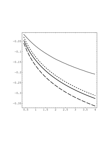
$R_{0}$

$\sqrt{s}\ (TeV)$

(c)

FIG. 6.: The ratio $R_{0}$ for $\gamma\gamma\to t\bar{t}$ versus the energy; SM (a), MSSM($\tan\beta=4$) (b); MSSM($\tan\beta=40$) (c); all logarithmic terms (solid), leading terms only (small dashed), leading angular independent terms only(large dashed); all logarithmic without Yukawa terms (very small dashed).

                              

$R_{0}$

$R_{0}$

$\sqrt{s}\ (TeV)$                                                                       $\sqrt{s}\ (TeV)$

(a)                                                                                    (b)

$R_{0}$

$\sqrt{s}\ (TeV)$

(c)

FIG. 7.: The ratio $R_{0}$ for $\gamma\gamma\to b\bar{b}$ versus the energy; SM (a), MSSM($\tan\beta=4$) (b); MSSM($\tan\beta=40$) (c); all logarithmic terms (solid), leading terms only (small dashed), leading angular independent terms only(large dashed); all logarithmic without Yukawa terms (very small dashed).

                              

$R_{0}$

$R_{0}$

$\sqrt{s}\ (TeV)$                                                                       $\sqrt{s}\ (TeV)$

(a)                                                                                    (b)

$R_{0}$

$\sqrt{s}\ (TeV)$

(c)

FIG. 8.: The ratio $R_{0}$ for $\gamma\gamma\to f\bar{f}$ versus the energy; $l^{+}l^{-}$ (a), $t\bar{t}$ (b), $b\bar{b}$ (c); SM (solid), MSSM ($\tan\beta=4$) (small dashed), MSSM ($\tan\beta=40$) (large dashed).

                              

$R_{33}$

$R_{33}$

$\sqrt{s}\ (TeV)$                                                                       $\sqrt{s}\ (TeV)$

(a)                                                                                    (b)

$R_{33}$

$\sqrt{s}\ (TeV)$

(c)

FIG. 9.: The ratio $R_{33}$ for $\gamma\gamma\to f\bar{f}$ versus the energy; $l^{+}l^{-}$ (a), $t\bar{t}$ (b), $b\bar{b}$ (c); SM (solid), MSSM ($\tan\beta=4$) (small dashed), MSSM ($\tan\beta=40$) (large dashed).

                              

$R_{2}$

$R_{2}$

$\sqrt{s}\ (TeV)$                                                                       $\sqrt{s}\ (TeV)$

(a)                                                                                    (b)

$R_{2}$

$\sqrt{s}\ (TeV)$

(c)

FIG. 10.: The ratio $R_{2}$ for $\gamma\gamma\to f\bar{f}$ versus the energy; $l^{+}l^{-}$ (a), $t\bar{t}$ (b), $b\bar{b}$ (c); SM (solid), MSSM ($\tan\beta=4$) (small dashed), MSSM ($\tan\beta=40$) (large dashed).

                              

$R_{3}$

$R_{3}$

$\sqrt{s}\ (TeV)$                                                                       $\sqrt{s}\ (TeV)$

(a)                                                                                    (b)

$R_{3}$

$\sqrt{s}\ (TeV)$

(c)

FIG. 11.: The ratio $R_{3}$ for $\gamma\gamma\to f\bar{f}$ versus the energy; $l^{+}l^{-}$ (a), $t\bar{t}$ (b), $b\bar{b}$ (c); SM (solid), MSSM ($\tan\beta=4$) (small dashed), MSSM ($\tan\beta=40$) (large dashed).

                              

$R_{23}$

$R_{23}$

$\sqrt{s}\ (TeV)$                                                                       $\sqrt{s}\ (TeV)$

(a)                                                                                    (b)

$R_{23}$

$\sqrt{s}\ (TeV)$

(c)

FIG. 12.: The ratio $R_{23}$ for $\gamma\gamma\to f\bar{f}$ versus the energy; $l^{+}l^{-}$ (a), $t\bar{t}$ (b), $b\bar{b}$ (c); SM (solid), MSSM ($\tan\beta=4$) (small dashed), MSSM ($\tan\beta=40$) (large dashed).

REFERENCES

• [1] Opportunities and Requirements for Experimentation at a Very High Energy $e^{+}e^{-}$ Collider, SLAC-329(1928); Proc. Workshops on Japan Linear Collider, KEK Reports, 90-2, 91-10 and 92-16; P.M. Zerwas, DESY 93-112, Aug. 1993; Proc. of the Workshop on $e^{+}e^{-}$ Collisions at 500 GeV: The Physics Potential, DESY 92-123A,B,(1992), C(1993), D(1994), E(1997) ed. P. Zerwas; E. Accomando etal Phys.Rep.C299,299(1998).
• [2] ” The CLIC study of a multi-TeV $e^{+}e^{-}$ linear collider”, CERN-PS-99-005-LP (1999).
• [3] P. Ciafaloni and D. Comelli, Phys. Lett. B 446, (1999), 278; M. Beccaria, P. Ciafaloni, D. Comelli, F.M. Renard and C. Verzegnassi, Phys. Rev. D61,073005(2000); M. Beccaria, P. Ciafaloni, D. Comelli, F.M. Renard and C. Verzegnassi, Phys.Rev. D61,011301(2000); M. Beccaria, F.M. Renard and C. Verzegnassi, hep-ph/0007224; to appear in Phys.Rev.D; M. Beccaria, F.M. Renard and C. Verzegnassi, Phys.Rev.D63,053013(2001) M. Beccaria, F.M. Renard and C. Verzegnassi, hep-ph/0103335.
• [4] J.H. Kühn, A.A. Penin, hep-ph/9906545.
• [5] V. V. Sudakov, Sov. Phys. JETP 3, 65 (1956); Landau-Lifshits: Relativistic Quantum Field theory IV tome, ed. MIR.
• [6] M. Kuroda, G. Moultaka and D. Schildknecht, Nucl.Phys. B350,25(1991); G.Degrassi and A Sirlin, Phys.Rev.D46,3104(1992); A. Denner, S. Dittmaier and R. Schuster, Nucl.Phys. B452,80(1995); A. Denner, S. Dittmaier and T. Hahn, Phys. Rev.D56,117(1997); W. Beenakker et al., Nucl.Phys.B410,245(1993) and Phys.Lett.B317,622(1993).
• [7] J.H. Kühn, A.A. Penin and V.A. Smirnov, Eur.Phys.J C17,97(2000).
• [8] P. Ciafaloni and D. Comelli, Phys.Lett.B 476,49(2000); M. Ciafaloni, P. Ciafaloni and D. Comelli, Nucl.Phys.589,359(2000) and Phys.Lett. B 501,216(2001).
• [9] W. Beenakker, A. Werthenbach, Phys,Lett.B489,148(2000); M. Hori, H. Kawamura and J. Kodaira, HUPD-003, hep-ph/0007329.
• [10] M. Melles, Phys.Lett. B 495,81(2000); V.S. Fadin, L.N. Lipatov, A.D. Martin and M. Melles, Phys.Rev.D61,094002(2000); M. Melles, hep-ph/000456,hep-ph/001196 and hep-ph/0012157.
• [11] A. Denner and S. Pozzorini, Eur.Phys.Jour.C18,461(2001) and hep-ph/0101213.
• [12] I.F. Ginzburg, G.L. Kotkin, V.G. Serbo and V.I. Telnov, Nucl. Instr. and Meth. 205, 47 (1983); I.F. Ginzburg, G.L. Kotkin, V.G. Serbo, S.L. Panfil and V.I. Telnov, Nucl. Instr. and Meth. 219,5 (1984); J.H. Kühn, E.Mirkes and J. Steegborn, Zeit.f.Phys.bf C57,615(1993).
• [13] V. Telnov, hep-ex/0003024, hep-ex/0001029, hep-ex/9802003, hep-ex/9805002, hep-ex/9908005; I.F. Ginzburg, hep-ph/9907549; R. Brinkman hep-ex/9707017. V. Telnov, talk at the International Workshop on High Energy Photon Colliders, http://www.desy.de/   gg2000, June 14-17, 2000, DESY Hamburg, Germany, to appear in Nucl.Instr. & Meth. A.; D.S. Gorbunov, V.A. Illyn, V.I. Telnov, hep-ph/0012175.
• [14] A. Denner, S. Dittmaier and M. Strobel, Phys.Rev D53,44,(1999);A. Denner and S. Dittmaier, Eur.Phys.J. C9,425,(1999).
• [15] M.L. Zhou et al, Phys.Rev.D61,033008(2000).
• [16] M. Jacob and G.C. Wick, Ann.Phys. 7,404(1959).
• [17] G. Passarino and M. Veltman, Nucl.Phys.B160,151(1979); K. Hagiwara, S. Matsumoto, D. Haidt and C.S. Kim, Zeit.f.Phys.C64,559(1995).
• [18] M. Beccaria, F.M. Renard and C. Verzegnassi, PM/01-18, hep-ph/0104245.
• [19] see e.g. G.J. Gounaris, P.I. Porfyriadis, F.M. Renard, hep-ph/9902230, Eur.Phys. Jour.C9,673(1999), and references therein.
Refer to caption
(a)
Refer to caption
(b)
Refer to caption
(c)