Abstract

We present parton distribution functions which include a quantitative estimate of its uncertainties. The parton distribution functions are optimized with respect to deep inelastic proton data, expressing the uncertainties as a density measure over the functional space of parton distribution functions. This leads to a convenient method of propagating the parton distribution function uncertainties to new observables, now expressing the uncertainty as a density in the prediction of the observable. New measurements can easily be included in the optimized sets as added weight functions to the density measure. Using the optimized method nowhere in the analysis compromises have to be made with regard to the treatment of the uncertainties.

1 Introduction

With the advent of new hadron collider experiments the need to quantitatively estimate parton distribution function (PDF) uncertainties is of paramount importance. One obvious example where the PDF uncertainty will become crucial is the $W$-boson mass uncertainty. By no means is this the only observable for which the PDF uncertainty is of the utmost importance.

The realization that hadron collider experiments had reached a level of accuracy where a quantitative approach towards the PDF uncertainties was needed came with the one-jet inclusive transverse energy distribution measurement of the CDF collaboration using the run 1a data with an integrated luminosity of 19.5 pb^-1 [1]. Up to that point the qualitative “global fitting” approach had worked well and was used to demonstrate the success of the perturbative QCD framework. Be that as it may, the precision of the CDF one-jet inclusive measurement demonstrated that the qualitative approach had reached its limit in usefulness. The fact that prior to the measurement none of the PDF’s could predict the high transverse momentum data whereas after the measurement the PDF’s could be adjusted to accommodate the high transverse energy excess [2] speaks for itself. The only way to continue is to use a quantitative approach which reflects the PDF uncertainties.

The qualitative “global fitting” approach [3, 4] combines a large amount of experimental data to form an error weighted average of all input data, i.e. find the minimum $\chi^{2}$ solution. In the calculation of the $\chi^{2}$ the experimental statistical and systematic uncertainties are added in quadrature. Because experiments are combined with each other, even if no statistical adequate solution could be found, no conventional probabilistic interpretation can be reached (see for instance section II.D of ref. [5] for an overview of the paradoxal problems encountered when attempting a probabilistic interpretation in the “global fitting” approach).

It is crucial to develop a rigorous statistical approach such that the uncertainties have an objective statistical interpretation and in case of deviations the experiments or prior assumptions causing the conflict are traceable. The apparent way to proceed would be to redo the “global fitting” approach with the uncertainty analysis in mind. That is, treating the experimental error analysis more carefully by including correlation matrices reflecting the experimental uncertainty and by demanding the input experiments to be compatible. As an advantage this would still allow a $\chi^{2}$ calculation with a minimalization procedure. The final result is then quoted as a correlation matrix of the PDF parameters, i.e. a 2nd order Taylor expansion around the best solution. Yet, this method has problems. First of all the experimental systematic uncertainties are not gaussian despite the fact that often gaussian approximations are published. Secondly, one can expect complicated correlations between the PDF parameters given the fact that the problem of PDF fitting is highly non-linear causing lower dimensional non-trivial regions in PDF parameter space with constant probability measure (i.e. constant $\chi^{2}$). Thirdly, in the end the PDF’s are not the physical observables and propagation from the PDF parameters to the physical observable would again necessitate a linearization of the error propagation involving an estimate of the derivative of the observable with respect to the PDF parameters. In short, this method has three layers of subsequent linearizations of uncertainties which can lead to problems.

The first paper using this method  [6] uses the H1, ZEUS, BCDMS and NMC data. Subsequently, refs. [7, 8] include additional experiments into the fits. Recently, a Lagrange multiplier method was outlined which does not need to make gaussian approximations [9]. Also proposed in refs  [9, 10] is a procedure to maintain the “global fitting” philosophy by include as many experiments as possible. To recover a probabilistic interpretation one has to multiply the experimental uncertainties with a common factor such that all experiments are consistent within a single PDF “global fit”.

Parallel to the previous methods, a different approach was pursued in ref. [11] to remove the last of the three gaussian approximations in the error analysis. Using the gaussian parameter probability density of ref. [6] an optimized Monte Carlo integration approach was applied to predict physical observables expressing its PDF uncertainty as a density probability measure in the predictions of the observable. Note that such an approach can be mathematically reformulated as a statistical inference method. In this paper we extend this method to eliminate all approximations in the error analysis. As a result any experimental error analysis can be implemented and the final resulting uncertainties for observables can assume any form. The intermediate PDF parameter probability distribution can have any shape required by the experiments. The resulting optimized Monte Carlo approach is transparent, easy to use, modular and extendible. These properties are important for practical use.

In section 2 we will explain our method of optimized Monte Carlo integration. After that we are ready to optimize the PDF’s towards sets of experiments. In section 3 we will consider the proton $F_{2}$ results of H1, ZEUS, BCDMS and NMC together with an world averaged value of $\alpha_{S}(M_{Z})$. The conclusions and outlook will be given in section 4.

2 The Method

This section will describe the methodology we developed to obtain theoretical predictions of physical observables including PDF uncertainties. Before we can formulate our method we need to define carefully all aspects of comparing experiments and theory. First of all, one has to define a theoretical framework which approximates the true nature value of observables. Secondly, the experimental results have to be casted in a well defined object which will take the form of an experimental response function. After defining the theoretical prior and the experimental response function we have the right language to formulate our method.

2.1 The Model Priors

Any observable has a true nature value $x_{T}$ which has to be calculated (i.e. approximated) by a theory model giving a value $x_{t}$. The PDF’s only consist within the framework of the parton model and perturbative QCD . This implies approximations have been made to arrive at this calculable model. Hence the resulting PDF’s will depend on the theory model defined in the prior. As long as the experimental uncertainties are larger than the deviations from the true nature value due to the theory model the approach is valid. The model uncertainties fall into three distinct classes.

The first class is an agglomeration of non-perturbative effects. One has to make the approximation in which factorizable PDF’s and calculable hard scattering matrix elements exist [12]. This leads to the appearance of power suppressed momentum transfer terms. These higher twist terms can be either parametrized (see e.g. ref. [7]) or assumed small enough to be neglectable by applying appropriate kinematic cuts. Moreover, the final state outgoing partons are assumed to have factorizable fragmentation functions. This again leads to power suppressed momentum transfer terms. Finally there is the interaction of the colliding hadron remnants with the hard scattering. For this effect no real physics models exist and usually the experiment is “corrected” for the “underlying event” fathering a large systematic uncertainty. For this paper we will neglect all such effects in the theory prior and assume they are neglectable with respect to the other uncertainties in play for the kinematic cuts applied. The underlying event subtraction is, as usual, considered an experimental problem. One final non-perturbative effect comes in play when experiments are considered which use other initial state hadrons than protons (e.g. deuterium, iron, copper, etc.). In such a case one has to consider the effect of the multitude of nuclei. That is, what is the relation between the free proton PDF and the measured atomic densities. In this paper we will not include heavy target data and therefore can ignore the phenomelogical shadow models which attempt to describe these nuclear effects. Note that the inclusion of non-perturbative models will involve the introduction of additional degrees of freedom (i.e. non-perturbative parameters). The effect is to de-emphasize certain kinematical regions associated with low momentum transfer scattering. Such non-perturbative models, if included in the theory prior, must be applied consistent to all predictions.

The second class of uncertainties is related to the perturbative expansion of the hard scattering partonic cross sections. Because this is in principal calculable the uncertainties are more traceable. In the theory prior one has to determine the order in perturbative QCD to which all observables will be calculated. This also defines the order to which the PDF evolution has to be performed. A special case would be to define a resummation scheme of dominant initial state logarithms to extend the kinematic range of reliable predictions. If such a scheme is adopted it should be applied to all predictions. Also such a scheme could affect and modify the evolution equations. For this paper we choose the next-to-leading order approximations in the $\overline{\mbox{MS}}$ renormalization/factorization scheme for all observables. For the appropriate evolution of the PDF’s the program QCDNUM was used [13] which accuracy is more than adequate for current phenomenology [14]. Note a theoretical uncertainty could be assigned to the fixed order hard scattering matrix element calculation which reflects an estimate of the deviation from the prediction to an even higher order calculation of the observable. This can take many forms and will be highly subjective. However, one can define such a prior and incorporate it easily in the uncertainty analysis. In this paper we restrict ourselves to only looking at the renormalization/factorization scale dependence of the next-to-leading order theory predictions. To do this we allow a floating renormalization/factorization scale in the optimalization procedure. Given enough orders in the perturbative expansion virtually no scale dependence would remain. However, at next-to-leading order there will be a scale dependence on the observables and therefore the PDF’s. The extend to which the scale can vary independent of the PDF probability measure indicates the need to increase the perturbative order of the matrix element calculation. Given enough experimental accuracy the fixed order calculation will fail. This will be reflected through the scale in a strong preference for a specific value of this scale.

The final class of model priors is a set of additional requirements. Some of them can be physics necessities, e.g. the PDF charge and momentum conservation sum rules. Others can be more speculative, for instance assumptions about small and large parton fraction behavior or introducing PDF moment constraints from lattice QCD (see e.g. [15]). Also, one could use a previous PDF optimalization as a prior and include additional experiments in the optimized PDF sets. Note that this requires that the prior optimalization results are consistent with the new experiments, i.e. that the inclusion leads to a refinement of the relevant region contributing to the functional integration in the functional space $V(\mbox{$\cal F$})$ of PDF’s $\cal F$. The most important constraint in this class are smoothness constraints on the actual PDF’s which must be introduced to regulate unconstrained fluctuations due to the discrete nature of experimental results. The most restrained introduction of some of these requirement is to define a specific parameterization for the functional form of the PDF’s depending on a fixed, finite number of parameters. Note however that this still requires an assumption on the initial probability density distribution of those parameters. For this paper we choose one such parameterization as is detailed in the next section. All in all, the constraints have to be quantified and assembled as a prior probability density function measure, $P_{prior}(\mbox{$\cal F$})$, over the PDF functional space $V(\mbox{$\cal F$})$.

2.2 The Experimental Response Function

Given the theory prior we now can make well defined approximations $x_{t}$ of the true nature value $x_{T}$ for any relevant observable. In order to interact with the experimental results we have to define the experimental response function

$$P_{exp}(x_{e}|\mbox{$\cal D$}(x_{t}))=P_{exp}(x_{e}|x_{o})\ ,$$ (1)

which is a probability density estimating the likelyhood of measuring $x_{e}$ given the theory prediction $x_{t}$ and detector response ${\cal D}$. The detector response is the deformation inflicted on the physics signal by the detector resulting in the measured signal $x_{o}=\mbox{$\cal D$}(x_{t})$. The systematic uncertainties are now defined as a probability density measure, $P_{sys}(\mbox{$\cal D$})$, over the functional space $V(\mbox{$\cal D$})$ of all potential detector responses for the observable and quantifies the understanding of the detector. Note that in principle the experimental response function has to be formulated before the actual measurement of the particular observable. Also, theory predictions can originate from any source and are not tied to a specific model in any way.

Often the detector response is specific to a particular measurement and not correlated with any other experiment under consideration. In that case we can integrate over the detector response functional space

$$P_{exp}(x_{e}|x_{t})=\int_{V(\mbox{$\cal D$})}d\,\mbox{$\cal D$}\ P_{exp}(x_{e}|\mbox{$\cal D$}(x_{t}))\times P_{sys}(\mbox{$\cal D$})\ ,$$ (2)

thereby simplifying the analysis. For instance, if the detector response probability function is parameterizable in a multi-gaussian the above integration would simplify to the usual $\chi^{2}$ formulation with a correlation matrix encapsulating the systematic uncertainties.

Note that if several measurements with correlated systematic uncertainties are included one has to integrate the systematic uncertainties over the group of correlated measurements. A more flexible approach is to use the optimized Monte Carlo approach (explained in the next subsection) not only for the PDF’s but in conjunction with the detector response $\cal D$. This way, each PDF has a specific detector response $\cal D$ which makes propagation of systematic uncertainties to other observables trivial.

The experimental response function $P_{exp}$ together with the detector response function $P_{sys}$ contains all information we can extract from the measurement. Together with the actual measured values of the observable, $x_{m}$, they form a permanent and well defined record of the measurement.

2.3 The Optimized Monte Carlo Approach

We now can formulate our method. To make a prediction for observable ${\cal O}$ which includes the PDF uncertainty based on prior assumptions and certain sets of measurements, we perform the integration over the PDF and detector response functional space to obtain the probability density function of observing a value $x_{e}$ for observable ${\cal O}$

$$P_{pdf}^{\cal O}(x_{e})=\int_{V(\mbox{$\cal F$})}d\,\mbox{$\cal F$}\ P_{exp}^{input}(\mbox{$\cal F$})\times P_{prior}(\mbox{$\cal F$})\times P_{exp}^{\cal O}\left(x_{e}|x_{t}(\mbox{$\cal F$})\right)\ ,$$ (3)

where $P_{exp}^{\cal O}\left(x_{e}|x_{t}(\mbox{$\cal F$})\right)$ is the experimental response function for observable ${\cal O}$ using PDF set $\cal F$. Note we have integrated out the systematic uncertainties for the observable as explained in eq. 2 and thereby assuming its systematic uncertainties are independent of the other experiments involved in the PDF determination. The prior probability function $P_{prior}$ is defined in subsection 2.1 and quantifies all prior PDF assumptions and regulators. Finally, the probability function of the input experiments is defined as

$$P_{exp}^{input}(\mbox{$\cal F$})=\int_{V(\mbox{$\cal D$})}d\,\mbox{$\cal D$}\ P_{exp\ 1}(\mbox{$\cal F$},\mbox{$\cal D$})\times P_{exp\ 2}(\mbox{$\cal F$},\mbox{$\cal D$})\times\cdots\times P_{exp\ n}(\mbox{$\cal F$},\mbox{$\cal D$})\times P_{sys}(\mbox{$\cal D$})\ ,$$ (4)

with the individual experimental response function for each experiment

$$P_{exp\ k}(\mbox{$\cal F$},\mbox{$\cal D$})=P_{exp\ k}\left(x_{m}^{(k)}\Big{|}\mbox{$\cal D$}\left(x_{t}^{(k)}(\mbox{$\cal F$})\right)\right)\ ,$$ (5)

where the actual measurement $x_{m}^{(k)}$ is substituted in the experimental response function. While formally this defines the PDF uncertainty for any observable we want, in practice a numerical integration over the PDF’s and possible systematic uncertainties has to be implemented. The only feasible method in this situation is a Monte Carlo approach. That is, we approximate the integral by randomly picking a sufficient large set of $N$ PDF’s and possible detector response functions such that

$$P_{pdf}^{\cal O}(x_{e})\approx\frac{1}{N}\sum_{i=1}^{N}P_{exp}^{input}(\mbox{$\cal F$}_{i})\times P_{prior}(\mbox{$\cal F$}_{i})\times P_{exp}^{\cal O}\left(x_{e}|x_{t}(\mbox{$\cal F$}_{i})\right)\ ,$$ (6)

and

$$P_{exp}^{input}(\mbox{$\cal F$}_{i})=P_{exp\ 1}(\mbox{$\cal F$}_{i},\mbox{$\cal D$}_{i})\times P_{exp\ 2}(\mbox{$\cal F$}_{i},\mbox{$\cal D$}_{i})\times\cdots\times P_{exp\ n}(\mbox{$\cal F$}_{i},\mbox{$\cal D$}_{i})\times P_{sys}(\mbox{$\cal D$}_{i})\ .$$ (7)

While this can be numerically implemented, the Monte Carlo integration efficiency defined as the ratio of the average of the combined probability function and the maximum of the combined probability function

$$\epsilon(P(\mbox{$\cal F$},\mbox{$\cal D$}))\approx\left(\frac{1}{N}\sum_{i=1}^{N}P(\mbox{$\cal F$}_{i},\mbox{$\cal D$}_{i})\right)\Big{/}\left(\max_{i}P(\mbox{$\cal F$}_{i},\mbox{$\cal D$}_{i})\right)\ ,$$ (8)

with

$$P(\mbox{$\cal F$},\mbox{$\cal D$})=P_{exp\ 1}(\mbox{$\cal F$},\mbox{$\cal D$})\times P_{exp\ 2}(\mbox{$\cal F$},\mbox{$\cal D$})\times\cdots\times P_{exp\ n}(\mbox{$\cal F$},\mbox{$\cal D$})\times P_{sys}(\mbox{$\cal D$})\times P_{prior}(\mbox{$\cal F$})\ ,$$ (9)

is for all practical purposes zero. This because given the virtually infinite functional space of choices of $\cal F$ and $\cal D$ the likelihood of choosing at random a set which gives a non-neglectable contribution to the functional integral is zero.

The standard method to tackle this problem is to optimize the Monte Carlo integration with respect to the combined probability function, i.e. “unweighting”. Looking at eq. 3 this procedure simply comes down to changing the integration measure by redefining the PDF’s $\cal F$ to $\mbox{$\cal F$}^{\prime}$ together with the detector response function $\cal D$ to $\mbox{$\cal D$}^{\prime}$ such that all the probability densities are absorbed in the integration measure. After such a transformation eqs. 3 and 4 simplify to

$$P_{pdf}^{\cal O}(x_{e})=\left(\int_{V(\mbox{$\cal F$}^{\prime})}d\,\mbox{$\cal F$}^{\prime}\ P_{exp}^{\cal O}\left(x_{e}|x_{t}(\mbox{$\cal F$}^{\prime})\right)\right)\int_{V(\mbox{$\cal D$}^{\prime})}d\,\mbox{$\cal D$}^{\prime}\ .$$ (10)

Translating this in the Monte Carlo integration approach now gives an efficiency of one, i.e. the Monte Carlo sets are “unweighted” and eqs. 6 and 7 transform in the trivial formula

$$P_{pdf}^{\cal O}(x_{e})\approx\frac{1}{N}\sum_{i=1}^{N}P_{exp}^{\cal O}\left(x_{e}|x_{t}(\mbox{$\cal F$}_{i}^{\prime})\right)\ ,$$ (11)

where the probability measure is quantified in the density of $(\mbox{$\cal F$}^{\prime}_{i},\mbox{$\cal D$}^{\prime}_{i})$ functional sets.

Note that we could also have optimized with respect to a subset of the experiments, e.g. experiments 2 through $n$. We would then find

$$P_{pdf}^{\cal O}(x_{e})\approx\frac{1}{N}\sum_{i=1}^{N}P_{exp\ 1}\left(x_{m}^{(1)}\Big{|}\mbox{$\cal D$}_{i}^{\prime}\left(x_{t}^{(1)}(\mbox{$\cal F$}_{i}^{\prime})\right)\right)P_{exp}^{\cal O}\left(x_{e}|x_{t}(\mbox{$\cal F$}_{i}^{\prime})\right)\ .$$ (12)

which tells us how to include an additional measurement, not included in the optimalization procedure. However, care has to be taken with the efficiency. The effective number of PDF’s used to estimate the observable is no longer $N$ but $N_{eff}=\epsilon(P_{exp\ 1})\times N$. If the efficiency is too low the Monte Carlo estimate uncertainty on the observable will become large and dominate over the PDF uncertainties. This can happen if the newly included experiment has a superior uncertainty analysis compared to the previous included experiments in which case one has to increase the initial number of sets $N$. Or, alternatively, the newly included experiment disagrees with the previous included experiments in which case the situation cannot be resolved by increasing $N$. Coercing the experiments together plainly leads to an incorrect result.

2.4 Comparison Methodology

As explained in section 2.3 the predictions are based on a discreet set of PDF’s and will build up a probability density in the space of the observable as is expressed in eq. 11. Note that the probability function density function of measuring $x_{e}$ for observable ${\cal O}$, $P^{\cal O}_{pdf}(x_{e})$, depends on the experimental response function of the measurement. Each discreet prediction will be “smeared” into a continuous probability function and averaged over all PDF’s in the set. This means that the particular form of the experimental response function dictates the minimum number of PDF’s needed for a satisfactory result. A drawback is that each experiment measuring the observable will have a different $P^{\cal O}_{pdf}$. In more theoretical studies one often wants a prediction independent of any particular experiment. In that case we have to substitute for the experimental response function an idealized detector model. The most straightforward model is the “perfect” detector, i.e.

$$P_{pdf}^{\cal O}(x_{e})\approx\frac{1}{N}\sum_{i=1}^{N}\delta(x_{e}-x_{t}(\mbox{$\cal F$}_{i}))$$ (13)

where the sum runs over the optimized PDF’s in the set. Such a result leads to a traditional scatter plot representation of $P^{\cal O}_{pdf}$. By introducing a averaging parameter $\Delta$ one can get to a more continues result. One could for instance use a gaussian with a width $\Delta$ for the response function. However, traditionally one chooses two theta functions to get a histogrammed representation of $P^{\cal O}_{pdf}$.

$$P_{pdf}^{\cal O}(x_{e})\approx\frac{1}{N}\sum_{i=1}^{N}\Theta(x_{e}-\frac{1}{2}\Delta-x_{t}(\mbox{$\cal F$}_{i}))\times\Theta(x_{t}(\mbox{$\cal F$}_{i})-x_{e}-\frac{1}{2}\Delta)\ .$$ (14)

The drawback of such procedures is that resulting approximation of $P_{pdf}^{\cal O}$ depends on the averaging procedure.

While the above procedures will give us an approximation for the probability density function of the observable it does not represent a likelyhood or confidence level. Using $P_{pdf}^{\cal O}(x_{e})$ it is pretty straightforward to construct the confidence level. However some care has to be taken given the potential non-gaussian nature of the experimental response function. First we define the parameter independent log-likelyhood

$$L^{2}(x_{e})=-2\times\log(P_{pdf}^{\cal O}(x_{e})/P_{expmax}^{\cal O}(x_{e}))\ ,$$ (15)

where

$$P_{expmax}^{\cal O}(x_{e})=\max_{x_{t}}P_{exp}^{\cal O}(x_{e}|x_{t})\ ,$$ (16)

is the maximum obtainable probability given an observed value $x_{e}$. For a gaussian response function the log-likelyhood defined here resorts back to the usual $\chi^{2}$ definition. The definition of log likelyhood as a ratio of probability densities has the property that it is independent under reparameterizations of the observable. We now can define the confidence level

$$CL^{\cal O}(x_{e})=\int d\,x\ \Theta(L^{2}(x)-L^{2}(x_{e}))\times P_{pdf}^{\cal O}(x)\$$ (17)

which is a proper probability. Given the measured value $x_{m}$, the confidence level $CL(x_{m})$ quantifies the probability that a repeat of the experiment will have a worse agreement with the theory prediction including the PDF uncertainties.

3 The Optimized Sets

The previous section defined the theory prior with the exception of the actual PDF parameterization. In subsection 3.1 the parameterization used for this paper will be discussed. Once that is done we perform in subsection 3.2 the actual optimalization using various combinations of proton $F_{2}$ and $\alpha_{S}$ measurements.

3.1 The Parameterization Choice

Given this is our first venture into the refractory subject of PDF determination we choose the well established MRST-parameterization [16] as our first guidance. This choice implicitly incorporates into the theory prior the accumulated knowledge of many years of PDF studies which can be considered a positive feature. However, because we have to adhere to the experimental systematic uncertainties and statistical interpretation of the results this parameterization can turn out to be far too restrictive. Such restrictive parameterizations might result in at least an underestimate of the PDF uncertainties. Or, more seriously, in discrepancies between the theory and the data stemming not from physics but from the parameterization choice. See for instance ref. [17] where the gluon PDF parameterization effects on the one jet inclusive transverse energy distribution are discussed.

For completeness, the explicit MRST-parameterization at the scale $Q_{0}=1$ GeV is given by

$$xu_{v} = A_{u}x^{-\lambda_{u}}(1-x)^{\eta_{u}}(1+\epsilon_{u}\sqrt{x}+\gamma_{u}x)\$$

$$xd_{v} = A_{d}x^{-\lambda_{d}}(1-x)^{\eta_{d}}(1+\epsilon_{d}\sqrt{x}+\gamma_{d}x)$$

$$xg = A_{g}x^{-\lambda g}(1-x)^{\eta g}(1+\epsilon_{g}\sqrt{x}+\gamma_{g}x)$$

$$xS\equiv 2x(\bar{d}+\bar{u}+\bar{s}) = A_{S}x^{-\lambda_{S}}(1-x)^{\eta_{S}}(1+\epsilon_{S}\sqrt{x}+\gamma_{S}x)$$

$$x\Delta\equiv x(\bar{d}-\bar{u}) = A_{\Delta}x^{-\lambda_{\Delta}}(1-x)^{\eta_{S}+2}(1+\gamma_{\Delta}x+\delta_{\Delta}x^{2})\ .$$ (18)

The normalization coefficients $A_{u}$, $A_{d}$ and $A_{g}$ are determined by the charge and momentum conservation sum rules. Both the charm and bottom quark PDF’s are generated through perturbative evolution from mass threshold. For the charm quark the threshold mass is set to 1.5 GeV, while the bottom quark threshold mass is chosen to be 4.5 GeV.

To conclude, using the MRST-parameterization the functional PDF integration of subsection 2.3 is reduced to an integration over 21 parameters (not counting the strong coupling constant $\alpha_{S}$ and squared renormalization/factorization scale $\mu$). The prior probability distribution of the parameters is chosen to be uniform. Next, we have to optimize the parameters according to the combined probability density function.

3.2 The $F_{2}^{proton}$ and $\alpha_{S}$ Data Optimized Sets

Given the choice to abstain for the moment from any non-perturbative modeling in the theory prior, we have to limit ourselves to proton target data. The study of heavy nuclei data by introducing a shadowing model is a subsequent step in the development of the PDF’s and will be taken in another paper. The five deep inelastic $F_{2}^{P}$ experiments we have selected so far are BCDMS [18], NMC [19], H1 [20], ZEUS [21] and E665 [22]. For the $\alpha_{S}$ measurement we take the value from ref [23]: $\mbox{$\alpha_{S}$}(M_{Z})=0.119\pm 0.003$. While this value is in fact a world average of sorts, we will indicate it in the fits as the “LEP” experiment. All the experiments are summarized in table 1 together with the relevant properties.

Experiment	Measurement	usable points	used $x$-range	error analysis
BCDMS	$F_{2}^{P}$	344	$7.0\times 10^{-2}$-0.75	gaussian
H1	$F_{2}^{P}$	188	$5.0\times 10^{-5}$-0.32	half gaussian
ZEUS	$F_{2}^{P}$	187	$6.3\times 10^{-5}$-0.51	gaussian
NMC	$F_{2}^{P}$	127	$8.0\times 10^{-3}$-0.50	gaussian
E665	$F_{2}^{P}$	53	$3.7\times 10^{-3}$-0.39	gaussian
LEP	$\alpha_{S}$	1	N.A.	gaussian

Table 1: A summary of relevant properties of experiments considered in this paper.

With the exception of H1, all other experiments quote a gaussianized analysis of the systematic uncertainties (i.e. a correlation matrix of the experimental errors is either quoted or can be calculated using the published results). The H1 $F_{2}^{P}$ measurement has 5 sources of systematic uncertainties quoted as $\pm 1\sigma$ deviations where for some of the sources the $\sigma_{+}$ is different from the $\sigma_{-}$. This means that for H1 we use the technique described in the previous section and numerically integrate over the systematic uncertainties by optimizing the PDF parameters together with the 5 detector model parameters of H1 using as the $P_{sys}(\mbox{$\cal D$})$ detector response function 5 half-gaussians depending on the detector model parameters. For the other 4 experiments the correlation matrix is used, i.e. the systematic uncertainties are integrated out analytically. This implies all potential correlations between the different $F_{2}^{P}$ experiments are ignored.

Because no higher twist models are in the theory prior we apply a cut on the momentum transfer and parton fractions in the $F_{2}^{P}$ data as suggested in ref. [16]: $Q^{2}>2$ GeV² and $W^{2}=Q^{2}\times\left(1/x-1\right)>10$ GeV².

Apart from optimizing the PDF integration over the 21+1 PDF parameters and, for H1, the 5 detector model parameters, we also include the squared renormalization/factorization scale as an optimalization parameter. As explained in subsection 2.1 the reason is twofold. First of all varying the scale amplifies the PDF uncertainty stemming from the fixed order perturbative expansion approximation. Secondly, the resulting optimized factorization/renormalization scale will indicate to which degree the theory model is applicable. A very narrow distribution indicating a failure of the model, a wide distribution indicating the model is appropriate. Note that we have chosen the initial squared scale probability distribution uniform.

To obtain an optimized set we use a Metropolis Algorithm [24] combined with a simulated annealing procedure [25]. We will discuss some of its potential shortcomings as they can affect the results. The first potential problem is the possibility of equivalent disconnected maxima. While the annealing should guard against finding local maxima and nudge the Metropolis walker to the global maximum it can happen that more than one maximum exists of roughly equal probability which are not connected by a likely path. Given the finite number of steps the Metropolis walker takes this can cause problems as the generated optimized PDF’s are concentrated on one of the maxima neglecting the others. A trail-and-error method of choosing different starting points for the Metropolis walker can be employed. However for a finite number of steps this does not guarantee the absence of a secondary maximum. The second problem arises from the choice of step size for the Metropolis walker. One wants to keep the step size small relative to the width of the probability function in order to maintain a good efficiency for generating optimized sets. However, this leads to correlations between PDF’s subsequently generated. A common sense approach is to pick a small randomly ordered subset out of the generated optimized PDF parameter points. As that might be, for complicated topologies, especially subspace regions of constant probability, a large number of PDF’s can be required to sample the entire region important to the functional integral.

Note that these potential problems in generating the optimized sets are numerical in nature and not a shortcoming of the employed method. Both problems disappear in the limit of an infinite number of steps. Any finite number of Metropolis steps leaves the potential for problems as described above. For now we use the FERMILAB PC-farm [26] to generate optimized sets of 100,000 PDF’s (i.e. PDF parameters). Out of the 100,000 sets smaller subsets of 100, 1,000 and 10,000 PDF’s are constructed by random selection from the larger list. For most practical applications 100 optimized PDF’s are already enough. For more complicated analysis additional optimized PDF’s might be necessary.

	H1	BCDMS	E665	ZEUS	NMC	LEP
H1-MRST set	-	67%	21%	0.5%	$<$0.1%	31%
BCDMS-MRST set	85%	-	23%	1.5%	$<$0.1%	0.5%
E665-MRST set	30%	82%	-	1.6%	1.0%	99%
ZEUS-MRST set	22%	$<$0.1%	5.0%	-	$<$0.1%	24%
NMC-MRST set	$<$0.1%	28%	1.5%	$<$0.1%	-	3.2%

Table 2: The confidence level of each experiment given the different sets. The name of the set is composed of all included experiments and the PDF parameterization choice.

The first optimalization to consider are with respect to the individual $F_{2}^{P}$ experiments. Given a set optimized to one of the experiments we can calculate the confidence level that the prediction using this set describe the other four experiments. The confidence level, as is detailed in section 2.4, is defined as the probability a repeat of the experiment would result in a worse agreement than the current agreement. Given this analysis we can conclude which experiments are compatible and can be considered in combined optimized sets. The results are listed in table 2. Note that because different experiments will have different experimental response functions and hence different PDF uncertainties the confidence level of experiment A given experiment B is different from the confidence level of experiment B given experiment A. A dramatic point in case can be seen in table 2 between the H1 and ZEUS experiment. From the results exposed in table 2 we conclude that both ZEUS and NMC cannot be combined with any other experiment as they produce their own distinct PDF sets. Both NMC and BCDMS prefer a much lower value of $\alpha_{S}$ than the LEP result. We can combine H1, BCDMS and E665 as each of these experiments predicts the other two with high confidence.

Given the confidence level results we have constructed, apart from the 5 sets using the individual $F_{2}^{P}$ data results, 7 additional PDF sets with different combinations of H1, BCDMS, E665 and LEP results. Note that we combine the $\alpha_{S}$ measurement with BCDMS even though the confidence level tells us it is not compatible. While inconsistent we do this to get PDF sets with a somewhat more stabilized and acceptable $\alpha_{S}$. Alternatively, we could have chosen to fix the value of $\alpha_{S}$ to a predetermined value in the physics prior.

With the twelve optimized sets we are now ready for comparisons with hadron collider data. Given this is the first kind of such an endeavor we can expect surprises which will guide us to the next step in the further development of PDF’s with uncertainties. In subsequent papers we will explore the phenomelogical implications for many hadron collider observables.

3.3 Some PDF set Results

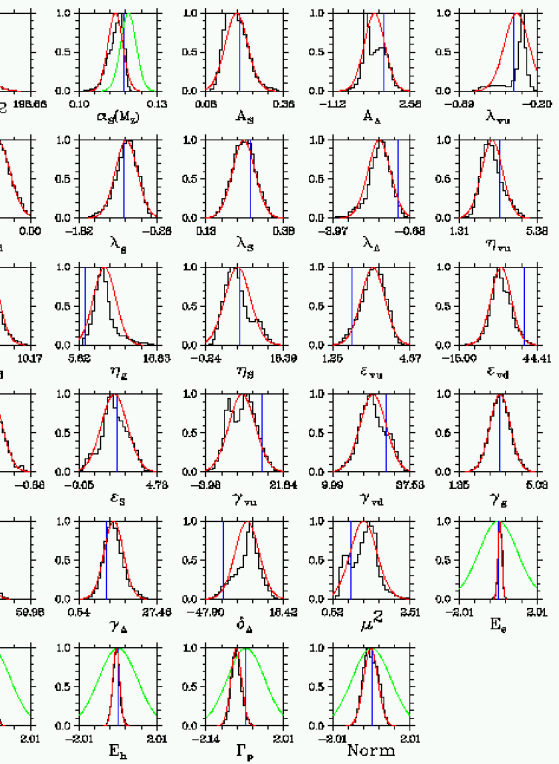
Figure 1: The H1-MRST set parameter distributions (histograms) together with the gaussian approximation (red curve) and the central MRST fit result [16] (blue bar). In addition the log-likelyhood $\Delta L^{2}$ distribution (histogram) and the $\chi^{2}$ probability distribution approximation (red curve) is shown. Note that the last 5 parameters are the detector model parameters of H1 [20] together with the prior probability distribution for this parameter (green curve). The green curve for the $\alpha_{S}$ result is the LEP value [23]

Given the factorization scheme dependence required for the calculation of the next-to-leading order matrix elements, the individual PDF’s do not contain much physics. Moreover the correlations between different PDF’s can be expected to be significant given the fact that at leading order the $F_{2}^{P}$ experiments only determine the squared electric charge weighted sum of the flavor PDF’s . At next-to-leading order one can hope at best to distinguish this charged sum of quark PDF’s from the gluon PDF. This renders a meticulous study of a specific flavor PDF prodigal. Yet, a cursory look might be helpful to understand the phenomelogical implications for hadron collider observables.

First of all we can look at the 21 PDF parameters of an optimized set together with $\alpha_{S}$, the squared renormalization/factorization scale and the log-likelyhood distribution. In fig. 1 we take as an example the H1-MRST optimized set which also includes the five detector modeling parameters. Prior to the optimalization each detector modeling parameters is given by a gaussian random parameter with an average of zero and a width of one. To obtain the fractional detector deformation of the $F_{2}^{P}$ signal a positive value of the random variable is multiplied by $\sigma_{+}$ and a negative value by $\sigma_{-}$. Examining fig. 1 we make several general observations which apply also to the other optimized set results:

• Many of the parameters deviate significantly from gaussian behavior, letting the linearized error propagation method of refs. [6, 7, 8] go astray.

• The central MRST fit [16] is not that far off for each individual parameter. The differences are attributed to the different treatment of the systematic errors and the MRST fit is averaged over many more experiments.

• The optimized detector response parameters are notably close to the H1 central value, though some of the distributions are skewed.

	$\alpha_{S}$-distribution	$\Delta L^{2}$-distribution
set	CL interval	$\min(\Delta L^{2})$	$\langle\Delta L^{2}\rangle$	$\frac{1}{2}\sigma^{2}(\Delta L^{2})$	NDP/DOF
ZEUS-MRST	(0.113,(0.114,(0.115),0.116),0.117)	466.1	481.2	42.9	187/23
NMC-MRST	(0.098,(0.102,(0.108),0.112),0.117)	185.4	196.4	10.1	127/23
H1-MRST	(0.108,(0.112,(0.115),0.117),0.119)	166.6	175.9	7.8	188/28
H1+LEP-MRST	(0.114,(0.116,(0.118),0.119),0.121)	167.3	176.0	8.3	189/28
BCDMS-MRST	(0.104,(0.106,(0.108),0.110),0.112)	317.2	328.1	12.1	344/23
BCDMS+LEP-MRST	(0.112,(0.113,(0.116),0.117),0.119)	325.0	335.8	15.7	345/23
E665-MRST	(0.106,(0.112,(0.116),0.127),0.133)	57.9	65.5	4.9	53/23
E665+LEP-MRST	(0.114,(0.117,(0.120),0.123),0.126)	59.1	66.5	6.0	54/23
H1+BCDMS-MRST	(0.109,(0.110,(0.112),0.114),0.115)	510.9	525.8	11.4	532/28
H1+BCDMS+LEP-MRST	(0.110,(0.111,(0.112),0.114),0.115)	511.5	521.8	10.0	533/28
H1+BCDMS+E665-MRST	(0.109,(0.111,(0.112),0.114),0.115)	580.3	596.2	12.3	585/28
H1+BCDMS+E665+LEP-MRST	(0.110,(0.112,(0.113),0.114),0.115)	579.7	592.3	10.4	586/28

Table 3: The relevant properties of the $\alpha_{S}$ and $\Delta L^{2}$ distributions for the optimized sets. The confidence level intervals are for a CL of 4.55%, 31.73% and 100%. The bin width used to calculate the confidence level intervals is 0.005 using the 1,000 PDF’s 

Also of interest are parameters not directly related to the PDF’s but important for the quality of the optimized set. These are the log-likelyhood distribution, the squared renormalization scale distribution and the $\alpha_{S}$ distribution for each of the twelve sets.

The value of $\alpha_{S}$ can be used to infer the reliability of the experimental error analysis. The confidence level intervals of the $\alpha_{S}$ distribution for all twelve PDF sets are listed in table 3. The notation used, $(a,(b,(c),d),e)$, is the following: the 100% confidence level interval is given by $c$ (i.e. the maximum value); the 31.73% confidence level interval is given by the interval $(b,d)$ (i.e. the “1-sigma” interval); the 4.55% confidence level interval is given by the interval $(a,e)$ (i.e. the “2-sigma” interval). In order to calculate the confidence level we use eq. 17 with $P_{pdf}^{\cal O}$ given by eq. 13:

$$CL(\mbox{$\alpha_{S}$})=\frac{1}{N}\sum_{i=1}^{N}\Theta\left(P_{pdf}(\mbox{$\alpha_{S}$}\left(\mbox{$\cal F$}_{i}\right))-P_{pdf}(\mbox{$\alpha_{S}$})\right)\ .$$ (19)

To evaluate the $P_{pdf}$ functions in the step function we have to measure the density of $\alpha_{S}$ predictions. To do this we choose the histogram approximation of eq. 14 with a width of 0.005. The number of PDF’s involved in the evaluation, $N$, is chosen to be 1,000. We can see the inclusion of $\alpha_{S}$ into the H1 and BCDMS optimalization pulls $\alpha_{S}$ towards the LEP value. For H1 it more than halves the uncertainty on $\alpha_{S}$, while for BCDMS the uncertainty is not affected much. This is understandable because the BCDMS result and the LEP result excluded each other up to a confidence level of 0.5%. Hence, coercing them into a combined optimalization has shifted the optimalization region and not, as is the case for the H1 optimalization, refined the optimalization region. For the sets combining several $F_{2}^{P}$ measurements we see that the inclusion of the LEP data point hardly affects the already well established value of $\alpha_{S}$. This can be understood by the large number of datapoints included in the combined experiments, rendering the uncertainty on $\alpha_{S}$ significantly smaller than the uncertainty on the LEP value of $\alpha_{S}$.

From the log-likelyhood we can deduct something about the quality of the optimalization. The log-likelyhood distribution is for all twelve sets close to the expected $\chi^{2}$ distribution. The relevant parameters are given in table 3. The minimum log-likelyhood, $\min(\Delta L^{2})$, found is on average equal to the number of data points (NDP) minus the degrees of freedom (DOF). However, due to the high degree of correlation between the PDF parameters the effective degrees of freedom (i.e. the independent degrees of freedom taking the correlations into account) is often much lower. The effective degrees of freedom are on average given by half the squared variance, $\frac{1}{2}\sigma^{2}(\Delta L^{2})$. The difference between the average value of the log-likelyhood, $\langle\Delta L^{2}\rangle$, and the minimum value is for a $\chi^{2}$ distributions equal to the effective number of independent parameters. From table 3 we can see that the ZEUS set and to a lesser extend the NMC set are problematic. This does not come as a surprise given the confidence level results of table 2.

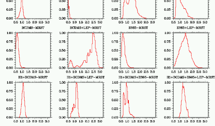
Figure 2: The squared renormalization/factorization scale distribution of the optimized sets. The horizontal axis is the squared ratio of the scale and the momentum transfer.

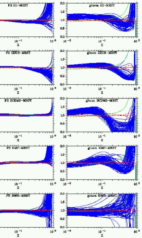
Figure 3: The ratio of the optimized PDF sets (blue) and CTEQ5M (green) over MRS99 at a scale of 10 GeV. The dashed red curves are the two MRS99 sets with $\alpha_{S}$$(M_{Z})$ values of 0.1125 and 0.1225. The left column is the charged summed combination of PDF’s , while the right column ratio of the gluon PDF .

Using the renormalization/factorization scale dependence one can deduce the applicability of the theory model. All 12 distributions are shown in fig. 2. The troubled ZEUS and NMC sets are also exposed here by the narrow range of optimized squared scales signaling a distress between the experimental result and the theory model. Yet, some of the other distributions are also worrisome indicating possibly a too restrictive parameterization choice. Note that while in the prior we assumed an uniform probability distribution for the squared scale, we restricted the range to be larger than half the squared momentum transfer $Q^{2}$ as we have a kinematic cut of $Q^{2}>2$ GeV² and a parameterization scale of $Q_{0}^{2}=1$ GeV².

Finally in fig. 3 we compare the optimized sets with the MRS99 [3] and CTEQ5M [4] distributions. This comparison forecasts the deviations we will see in the hadron collider observables between the global fitter predictions and the optimized PDF sets. As can be seen the squared charged sum of the flavored PDF’s agrees pretty well with MRS99 and CTEQ5M up to the point where there is data. Some subtle differences are present in some of the sets. The big difference however is the gluon distribution which is much lower above a parton fraction of 0.1 and higher between 0.01 and 0.1. These differences are consistent for all optimized PDF sets using the $F_{2}^{P}$ data and will be reflected in the phenomenology at hadron colliders.

It is interesting to note that the differences in the gluon PDF are especially large when compared with CTEQ5M. This gives us a first hint at the origin of differences with the optimized sets. The relevant difference between MRS99 and CTEQ5M is the choice of experiment to constrain the gluon PDF in the large $x$ region. The MRS99 global fit makes the traditional choice of using the WA70 [27] prompt photon data. Because the prompt photon data suffers from large theoretical uncertainties the CTEQ5M global fit instead chose the one jet inclusive transverse jet energy data of CDF and D0 [28, 29]. Yet the deep inelastic proton data favors the MRS99 over the CTEQ5M global fit result for large $x$ gluons. This is a rather troubling conclusion as it suggests a very significant deviation between the deep inelastic proton data and high transverse energy jet data at the TEVATRON.

4 Conclusions and Outlook

In this paper we introduced a flexible method to incorporate PDF uncertainties into phenomelogical predictions of collider observables. By representing the uncertainties as a density, i.e. an ensemble of PDF’s with which one predicts the observable, the practical use is both convenient and flexible. The sets used in this paper can be obtained from the website pdf.fnal.gov.

The restriction to a minimum set of experiments to determine the optimized PDF’s is deliberate as many experiments do not seem to be consistent with a single optimized PDF set. One of the next steps in developing the optimized PDF’s is to consider deuterium data and the related nuclear effects in the optimalization. While for deuterium the nuclear effects are small and manageable within the context of PDF optimalization, one can expect serious complications if one considers heavier targets. It might be better to use the optimized PDF’s to predict these measurements in order to obtain better understanding of the nuclear effects.

In the current optimized sets the most severe prior assumption is due to the restrictive MRST parameterization. One can argue the seemingly discrepancies between proton $F_{2}$ measurements and high energy jet production at CDF and D0 is due to the restrictive parameterization. It is therefore crucial to device more general schemes for parameterizing the PDF functionals. One way is to use complete sets of functions, in such a way that the higher order functions are associated with smaller scale fluctuation. The drawback of such methods is that changes in a parameter affect the PDF for all values of the parton fractions $x$. This induces strong correlations between the parameters and more importantly accurate data in localized regions of $x$ will affect the uncertainty estimates for all regions of $x$. A better method would be splines or other methods of generating functions using the value of the PDF at fixed grid points $x_{i}$. In such a case the parameters (i.e. the value at the grid points) are more localized. Such methods are under development and the subject of future publications.

Using the current optimized PDF sets a series of studies on hadron collider observables will be published. These studies range from luminosity measurements using $W$-boson and $Z$-boson cross sections to jet production. Given the upcoming run II at Fermilab and the LHC program at Cern further development of the optimized PDF’s is more than warranted as it will have a large impact on the phenomenology at these hadron colliders.

References

- [1] The CDF collaboration, hep-ex/9601008 (Phys. Rev. Lett. 77 (1996) 438).
- [2] J. Huston, E. Kovacs, S. Kuhlmann, H. L. Lai, J. F. Owens, D. Soper and W. K. Tung, hep-ph/9511386 (Phys. Rev. Lett. 77 (1996) 444).
- [3] A. D. Martin, R. G. Roberts, W. J. Stirling and R. S. Thorne, hep-ph/9906231 (Nucl. Phys. Proc. Suppl. 79 (1999) 105).
- [4] H. L. Lai, J. Huston, S. Kuhlmann, J. Morfin, F. Olness, J. F. Owens, J. Pumplin and W. K. Tung, hep-ph/9903282 (Eur. Phys. J. C12 (2000) 375).
- [5] The Structure Function Subgroup Summary, hep-ph/9706470 (Snowmass 1996 Workshop: New Directions for High Energy Physics).
- [6] S. Alekhin, hep-ph/9611213 (Eur. Phys. J. C10 (1999) 395).
- [7] M. Botje, hep-ph/9912439 (Eur. Phys. J. C14 (2000) 285).
- [8] V. Barone, C. Pascaud and F .Zomer, hep-ph/0004268.
- [9] D. Stump, J. Pumplin, R. Brock, D Casey, J. Huston, J. Kalk, H. L. Lai and W. K. Tung, hep-ph/0101051.
- [10] D. Stump, J. Pumplin, R. Brock, D Casey, J. Huston, J. Kalk, H. L. Lai and W. K. Tung, hep-ph/0101032.
- [11] W. Giele and S. Keller, hep-ph/9803393 (Phys. Rev. D58 (1998) 094023).
- [12] J. C. Collins, D. E. Soper and G. Sterman, Phys. Lett. B134 (1984) 263.
- [13] M. Botje, QCDNUM version 16.12, ZEUS-97-066 (unpublished).
- [14] J. Blümlein, M. Botje, C. Pascaud, S. Riemersma, W. L. van Neerven, A. Vogt and F. Zomer, hep-ph/9609400 (to appear in the proceedings of the workshop “Future Physics at HERA”, DESY, Hamburg, 1996).
- [15] M. Guagnelli, K. Jansen and R. Petronzio, hep-lat/9809009 (Nucl. Phys. B542 (1999) 395); hep-lat/9903012, (Phys. Lett. B459 (1999) 594).
- [16] A. D. Martin, R. G. Roberts, W. J. Stirling and R. S. Thorne, hep-ph/9803445 (Eur. Phys. J. C4 (1998) 463).
- [17] H. L. Lai, J. Huston, S. Kuhlmann, F. Olness, J. Owens, D. Soper, W. K. Tung and H. Weerts, hep-ph/9606399 (Phys. Rev. D55 (1997) 1280).
- [18] The BCDMS Collaboration, CERN-EP-89-06 (preprint contains the actual tabulated systematic uncertainties), Phys. Lett. B223 (1989) 485.
- [19] The NMC collaboration, hep-ph/9509406 (Phys. Lett. B364 (1995) 107).
- [20] The H1 collaboration, hep-ex/9603004 (Nucl. Phys. B470 (1996) 3).
- [21] The ZEUS collaboration, hep-ex/9607002 (Z. Phys. C72 (1996) 399).
- [22] The E665 collaboration, Phys. Rev. 54 (1996) 3006.
- [23] S. Bethke, hep-ex/0001023 (lecture given at Intern. Summer School at Nijmegen, August 1999).
- [24] N. Metropolis, N. Rosenbluth, A. Rosenbluth, M. Teller and E. Teller, Journal of Chemical Physics vol. 21, (1953) 1087.
- [25] S. Kirkpatrick, C. D. Gelatt and M. P. Vecchi, Science vol. 220 (1983) 671; S. Kirkpatrick, Journal of Statistical Physics vol 34 (1984) 975.
- [26] The FERMILAB PC-farm group.
- [27] The WA70 Collaboration, Z. Phys. C38 (1988) 371.
- [28] The CDF Collaboration, hep-ph/0102074.
- [29] The D0 Collaboration, hep-ex/0012046 (submitted to Phys. Rev. D).