Phase transition dynamics in the hot Abelian Higgs model

Abstract

We present a detailed numerical study of the equilibrium and non-equilibrium dynamics of the phase transition in the finite-temperature Abelian Higgs model. Our simulations use classical equations of motion both with and without hard-thermal-loop corrections, which take into account the leading quantum effects. From the equilibrium real-time correlators, we determine the Landau damping rate, the plasmon frequency and the plasmon damping rate. We also find that, close to the phase transition, the static magnetic field correlator shows power-law magnetic screening at long distances. The information about the damping rates allows us to derive a quantitative prediction for the number density of topological defects formed in a phase transition. We test this prediction in a non-equilibrium simulation and show that the relevant time scale for defect formation is given by the Landau damping rate.

DAMTP-2001-28 SUSX-TH-01-015

I Introduction

Whilst there are many useful techniques for studying the equilibrium properties of finite-temperature field theories, understanding the non-equilibrium dynamics is a much harder task. Nevertheless, it would be essential for many fields of physics, for instance cosmology, heavy ion physics and condensed matter physics. In all these fields, new empirical data will be available in near future, which would allow the theories to be tested, but the complexity and the non-equilibrium nature of the phenomena make it difficult to derive theoretical predictions that could be compared with the data.

One fairly generic consequence of phase transitions is formation of topological defects [1, 2]. If the phase transition is associated with a spontaneous breakdown of a global symmetry, this process is well understood. The correlation length of the order parameter cannot keep up with its equilibrium value, which diverges at the transition point. The direction of the symmetry breaking must therefore be uncorrelated at long distances, and at places where these correlated domains meet, topological defects are formed. This is called the Kibble-Zurek (KZ) mechanism (see e.g. [3] for a review).

If the symmetry that gets broken is a local gauge invariance, the above argument cannot be used directly, because the direction of the order parameter is not a gauge invariant quantity. We studied this recently in the context of the Abelian Higgs model [4], and pointed out that the thermal fluctuations of the magnetic field lead to another mechanism that forms topological defects. The argument was based on fairly generic assumptions, but leads to some concrete predictions that were confirmed in numerical simulations.

The aim of this paper is to study in more detail the dynamics of the Abelian Higgs model during the phase transition from the Coulomb phase to the Higgs phase. In particular, we concentrate on those degrees of freedom that are relevant for defect formation. This allows us to test the scenario of Ref. [4] on a more quantitative level.

The theory considered in Ref. [4] was classical, and although the same arguments apply to the quantum theory as well, the details of the dynamics are different. The full quantum field theory cannot be simulated in practice, but one can argue that the dynamics of the relevant long-wavelength degrees of freedom are classical [5]. By integrating out the short-wavelength fluctuations perturbatively, one obtains a classical effective theory with non-local interactions [6, 7, 8, 9], to which we refer as the hard-thermal-loop (HTL) improved theory. In order to understand how the quantum effects change the dynamics, we simulate this HTL improved theory using the method developed in Ref. [10].

The structure of the paper is the following: in Sect. II we present both the classical and HTL improved Abelian Higgs models. In Sect. III we discuss defect formation in the model, comparing the mechanism presented in [4] with the Kibble-Zurek scenario. In Sects. IV and V we describe our numerical simulations and present the results. Conclusions are given in Sect. VI and technical details of the HTL improved equations of motion and the lattice formulation in the two Appendices.

II Abelian Higgs model

The Abelian Higgs model is defined by the Lagrangian

$${\cal L}=-\frac{1}{4}F_{\mu\nu}F^{\mu\nu}+|D_{\mu}\phi|^{2}-m^{2}|\phi|^{2}-\lambda|\phi|^{4},$$ (1)

where $D_{\mu}=\partial_{\mu}+ieA_{\mu}$ and $F_{\mu\nu}=\partial_{\mu}A_{\nu}-\partial_{\nu}A_{\mu}$.

A particularly interesting feature of this theory is the existence of Nielsen-Olesen vortex solutions [11]. These string-like topological defects are characterized by a zero of the Higgs field at the centre of the vortex around which the Higgs phase angle has a non-zero winding number

$$n_{C}=\int_{C}d\vec{r}\cdot\nabla\gamma(\vec{r})\neq 0.$$ (2)

Here $C$ is a closed path around the vortex and $\gamma$ is the Higgs phase angle, i.e., $\phi=|\phi|\exp(i\gamma)$.

At finite temperature, perturbation theory is plagued by infrared divergences [12], which can be partly cured by a resummation of the perturbative expansion, but even the resummed expansion breaks down near the transition. Static equilibrium quantities, such as the phase diagram of the theory, can still be calculated reliably with non-perturbative Monte Carlo simulations.

The model has a phase transition between the high-temperature Coulomb phase and the low-temperature Higgs phase at $T^{2}=T_{c}^{2}\approx 12(-m^{2})/(3e^{2}+4\lambda)$. In the perturbative regime ($\lambda\ll e^{2}$), the transition is of first order [13], and at larger $\lambda$ it becomes continuous [14]. There are no local order parameters, but a number of non-local ones: the photon mass and the vortex tension are non-zero in the broken phase and vanish at the transition [15]. Therefore the transition is not a smooth crossover like the electroweak phase transition [16].

Monte Carlo simulations cannot be used for real-time quantities in the quantum theory, because the necessary path integral is not Euclidean but consists of a complicated path in complex time [17]. However, we can utilize the fact that modes with different momenta behave in very different ways [5]. The soft, long-wavelength modes ($k\ll T$) have large occupation numbers, and they can be approximated very well by a classical theory. This makes numerical simulations feasible, because the time-evolution of a classical field theory can be found simply by solving the equations of motion numerically.

A Classical theory at finite temperature

Classical field theory at finite temperature is ultraviolet divergent, and thus the results depend on the lattice spacing $\delta x$. Divergences like these are generic to all low-energy effective theories, and are exactly cancelled by corrections the high-momentum modes induce to the effective Lagrangian. If one is only interested in static equilibrium quantities, these corrections can be calculated in the limit of high temperature and small lattice spacing $\delta x$ [18, 19],

$$m_{T}^{2}=m^{2}+(3e^{2}+4\lambda)\left(\frac{T^{2}}{12}-\frac{3.176T}{4\pi\delta x}\right).$$ (3)

The approach we use in Sect. IV is to take this correction into account and solve the classical equations of motion

$$\partial_{\mu}F^{\mu\nu} = -2e{\rm Im}\phi^{*}D^{\nu}\phi,$$ (4)

$$D_{\mu}D^{\mu}\phi = -m_{T}^{2}\phi-2\lambda(\phi^{*}\phi)\phi.$$ (5)

However, as was pointed out in Ref. [20], these equations do not reproduce the real-time dynamics of the quantum theory correctly. Thus, the results are not reliable on a quantitative level, but they can still give a reasonably good qualitative picture of the dynamics, and provide a non-trivial test for the scenario presented in Section III.

B HTL improved theory

If the couplings are small, the system is close to thermal equilibrium and $T\delta x\gg 1$, it is possible to construct a classical theory which approximates the dynamics of the original quantum theory to leading-order accuracy in the coupling constants [9].

Near the phase transition, $m^{2}\sim-e^{2}T^{2}$, and we can use the high temperature approximation $T\gg m$ in our loop integrals, provided $e$ is small. We calculate the one-loop corrections from the hard modes to the self-energies of $\phi$ and $A_{i}$, and resum them into the effective Lagrangian [21]

$${\cal L}_{\text{HTL}} = -\frac{1}{4}F_{\mu\nu}F^{\mu\nu}-\frac{1}{4}m_{D}^{2}\int\frac{d\Omega}{4\pi}F^{\mu\alpha}\frac{v_{\alpha}v^{\beta}}{(v\cdot\partial)^{2}}F_{\mu\beta}$$ (7)

$$+|D_{\mu}\phi|^{2}-m_{T}^{2}|\phi|^{2}-\lambda|\phi|^{4},$$

where $m_{T}^{2}$ is given by Eq. (3), and the integration is taken over the unit sphere of velocities $v=(1,\vec{v})$, $\vec{v}^{2}=1$. The Debye mass has the value $m_{D}^{2}=\frac{1}{3}e^{2}T^{2}+\delta m_{D}^{2}$, where $\delta m_{D}^{2}$ is a counterterm that cancels the UV divergences and is discussed in more detail in Appendix B 2.

All the degrees of freedom remaining in this effective theory are classical, and therefore it can be treated as a classical theory. The time evolution of the fields will then be determined by the equations of motion [cf. Eq. (5)]:

$$\partial_{\mu}F^{\mu\nu} = m_{D}^{2}\int\frac{d\Omega}{4\pi}\frac{v^{\nu}v^{i}}{v\cdot\partial}E^{i}-2e{\rm Im}\phi^{*}D^{\nu}\phi,$$ (8)

$$D_{\mu}D^{\mu}\phi = -m_{T}^{2}\phi-2\lambda(\phi^{*}\phi)\phi.$$ (9)

As such, the equations of motion (9) are not well suited for our purposes. Firstly, it is not obvious how to find the corresponding Hamiltonian, which is necessary for preparing the initial configurations. And secondly, the equations of motion are non-local both in space and time.

In Ref. [10], a convenient local formulation was presented along the lines of Ref. [8]. The latter work introduces a new local field $W(t,\vec{x},\vec{v})$, representing the departure from the equilibrium distribution function for hard particles with velocity $\vec{v}$. Since the hard particles move at the speed of light, $\vec{v}$ consists of two free coordinates, making $W$ a six-dimensional field. In our formulation, part of the velocity dependence decouples from the dynamics of the soft modes, and we can describe exactly the same dynamics with two five-dimensional fields, $\vec{f}(t,\vec{x},z)$ and $\theta(t,\vec{x},z)$, where $z\in[0,1]$ is the cosine of the angle between the hard mode velocity and the gradient of the distribution function. The details of this formulation are given in Appendix A.

In order to simulate the model numerically, we define the theory on a periodic spatial lattice, and the $z$ dependence of $\vec{f}$ and $\theta$ is discretized by expressing them as sums over a finite number of Legendre modes, whose order ranges from $0$ to $N_{\rm max}$ [10]. The resulting equations of motion are detailed in Appendix A. We merely note here that, as shown in Ref. [10], for a given value of $N_{\rm max}$ and a given momentum $k$, the approximation breaks down at times

$$t\mathop{\raise 1.29167pt\hbox{$>$\kern-7.5pt\raise-4.73611pt\hbox{$\sim$}}}t_{c}(k)=4N_{\rm max}/k.$$ (10)

Therefore one can strictly speaking only measure correlators up to $\Delta t\sim N_{\rm max}\delta x$, but since the modes that are in equilibrium will remain in equilibrium even beyond that, one can essentially trust the results until $\Delta t\approx t_{c}(k)$, where $k$ is the relevant momentum scale.

In Sect. V, we study the dynamics of the model using the HTL improved equations of motion, and describe how these corrections change the results from the classical case.

III Defect formation

In cosmology, temperature of the universe decreases as a result of its expansion, and this leads to phase transitions. If we write the equations of motion in conformal coordinates, the effect of the expansion can be absorbed completely into a varying zero temperature Higgs mass term, $m^{2}=m^{2}(t)$.

In order to see this, we perform the conformal rescaling $dx^{\mu}\to adx^{\mu}$, $v^{\mu}\to av^{\mu}$, $A_{\mu}\to a^{-1}A_{\mu}$ and $\phi\to a^{-1}\phi$, where $a=a(t)$ is the scale factor of the Universe. If we can neglect the expansion rate in comparison to the microscopic timescales of the theory, which are given by $m_{T}^{-1}$ and $m_{D}^{-1}$, the effect of this rescaling on the action is to replace the mass terms $m_{T}^{2}$ and $m_{D}^{2}$ by $(m_{T}a)^{2}$ and $(m_{D}a)^{2}$ respectively. The hard modes are assumed to be ultra-relativistic, so they will stay close to a thermal distribution with temperature $T=\bar{T}a^{-1}$. Hence $(m_{D}a)^{2}$ stays constant, as do the rescaled thermal corrections to the Higgs mass, leaving the only time dependence in the parameter $m^{2}(t)=m^{2}a^{2}(t)$. In the following, we will assume that the phase transition is triggered in this way, by a mass term decreasing below a critical value, but we believe that the qualitative features would not be very different if some of the other parameters were changing at the same time.

When the system enters the Higgs phase, Nielsen-Olesen vortices are formed. In the limit $e\rightarrow 0$, this can be understood in terms of the Kibble mechanism [1]. When $m^{2}$ approaches its critical value, the Higgs correlation length $\xi$ grows, and if the system could remain in equilibrium it would eventually diverge at the transition point. However, $\xi$ cannot grow arbitrarily fast, because at the very least it is constrained by the finite speed of light. Therefore it remains finite if the transition takes place in finite time. At the transition point, the system consists of correlated domains of size $\hat{\xi}$ determined by the maximum correlation length reached. In each of these domains, the phase angle of the Higgs field is chosen independently of all others, and this gives rise to frustrations, vortices, where these domains meet. Up to a numerical factor, the number of vortices piercing a unit area is

$$n=N/A\approx\hat{\xi}^{-2}.$$ (11)

In practice, the maximal rate of change of the correlation length may be well below the speed of light, and this argument can indeed be made more precise by considering the dynamics of the system in more detail [22, 3].

In Ref. [4], we argued that this picture is not complete if $e>0$. After all, the phase angle of the Higgs field is not gauge invariant, and therefore arguments based on it cannot apply. Nevertheless, if the amplitude of the magnetic field is small, we can fix the gauge in which $A_{i}\approx 0$, and then we can use the above picture in this gauge. In these cases the above Kibble-Zurek scenario should work. However, if the initial state is at a non-zero temperature, magnetic field is never exactly zero, and it must be taken into account.

In the symmetric phase, the thermodynamics of the gauge field is described by ordinary electrodynamics. The energy of any magnetic field configuration is approximately given by

$$H_{\rm EM}[\vec{B}(\vec{x})]=\frac{1}{2}\int d^{3}x\vec{B}(\vec{x})^{2},$$ (12)

and the probability with which the thermal fluctuations can generate that configuration is proportional to $\exp(-H_{EM}/T)$. Let us consider a circular loop $C$ that bounds a surface $S$. The magnetic flux through the surface is

$$\Phi_{S}=\int d{\vec{S}}\cdot\vec{B}.$$ (13)

Although this is zero on the average, it is non-zero in almost all configurations, and therefore the typical value, given by $\sqrt{\Phi_{S}^{2}}$ is non-zero. We can estimate its value by calculating the energy of the field configuration that minimizes the energy for a given value of $\Phi_{S}$. This minimal configuration is simply a magnetic dipole, and its energy is

$$E_{\rm min}(\Phi_{S})\approx\Phi_{S}^{2}/R,$$ (14)

where $R$ is the radius of the loop $C$. Thermal fluctuations can create this configuration if $T\mathop{\raise 1.29167pt\hbox{$>$\kern-7.5pt\raise-4.73611pt\hbox{$\sim$}}}E_{\rm min}(\Phi_{S})$, and solving this for $\Phi_{S}$ shows that the typical flux through the loop is

$$\Phi_{S}\approx\sqrt{TR}.$$ (15)

When the system enters the Higgs phase, magnetic flux is confined into flux tubes, which costs energy. Therefore the dynamics tries to decrease the magnetic flux, but it can only do so at short distances, because the range of the interaction between the flux tubes decreases rapidly.

We can be more specific in Fourier space. We can write the two-point correlator of the magnetic flux density $\vec{B}$ as

$$\langle B_{i}(\vec{k})B_{j}(\vec{k}^{\prime})\rangle=\left(\delta_{ij}-\frac{k_{i}k_{j}}{k^{2}}\right)(2\pi)^{3}\delta(\vec{k}+\vec{k}^{\prime})G(k).$$ (16)

In the symmetric phase, different Fourier modes $\vec{B}(\vec{k})$ behave as independent oscillators in thermal bath, and thus each of them has the same amplitude $G_{0}(k)=T$. When the system enters the broken phase, magnetic field becomes massive, and the equilibrium distribution changes into

$$G(k)=T\frac{k^{2}}{k^{2}+m_{\gamma}^{2}}.$$ (17)

In order to stay in equilibrium, the amplitude of the long-wavelength modes must drop rapidly, but the time scale $\tau(k)$ of the dynamics of these modes is very slow. It depends on the individual system, but in general $\lim_{k\rightarrow 0}\tau(k)=\infty.$ Thus the modes with $k$ less than some critical value $\hat{k}$ cannot remain in equilibrium. If we know $\tau(k)$, we can calculate $\hat{k}$ from the condition

$$\left|\frac{d\ln G(\hat{k})}{dt}\right|\approx\frac{1}{\tau(\hat{k})}.$$ (18)

The consequence of the above process is that there will be long-wavelength magnetic fields present even in the Higgs phase. In particular, at distances less than $\hat{\xi}=2\pi/\hat{k}$ it looks like there was a uniform external magnetic field. We can estimate that its amplitude $B_{\rm avg}$ is

$$B_{\rm avg}^{2}\approx\left\langle\int_{0}^{\hat{k}}\frac{d^{3}k}{(2\pi)^{3}}B_{i}(\vec{k})\int_{0}^{\hat{k}}\frac{d^{3}k^{\prime}}{(2\pi)^{3}}B_{i}(\vec{k}^{\prime})\right\rangle\approx\int_{0}^{\hat{k}}\frac{d^{3}k}{(2\pi)^{3}}G_{0}(k)\sim T\hat{k}^{3}.$$ (19)

This magnetic flux must be confined into vortices, and because each vortex carries one flux quantum $\Phi_{0}=2\pi/e$, the number density of vortices per unit area is

$$n\approx\frac{e}{2\pi}B_{\rm avg}\approx\frac{e}{2\pi}T^{1/2}\hat{k}^{3/2}.$$ (20)

Even if we do not know $\tau(k)$, we can still make some concrete predictions based on this scenario. For instance, the spatial distribution of vortices turns out to be completely different than in the KZ scenario. At distances shorter than $\hat{\xi}=2\pi/\hat{k}$, the magnetic field points in the same direction, which means that the vortices tend to be aligned, while in the KZ scenario they prefer to be anti-aligned. This prediction was confirmed in the simulations in Ref. [4].

IV Classical simulations

A Equilibrium

In order to test the scenario presented in Sect. III, we carried out a number of numerical simulations. Let us first discuss the simulations of the classical model (5).

Because we are interested in transitions that start from close to thermal equilibrium, we will first have to thermalize the system. This means preparing an ensemble of field configurations with the canonical equilibrium distribution $\exp(-\beta H)$, where $\beta=1/T$ and the Hamiltonian $H$ is

$$H=\int d^{3}x\left[\frac{1}{2}\vec{E}^{2}+\frac{1}{2}(\vec{\nabla}\times\vec{A})^{2}+\pi^{*}\pi+(D_{i}\phi)^{*}(D_{i}\phi)+m_{T}^{2}\phi^{*}\phi+\lambda(\phi^{*}\phi)^{2}\right].$$ (21)

Here $\pi=\partial_{0}\phi$ is the canonical momentum of $\phi$, and in the temporal gauge ($A_{0}=0$), the electric field is simply $\vec{E}=-\partial_{0}\vec{A}$. In addition, the fields must satisfy the Gauss law as an extra constraint

$$\vec{\nabla}\cdot\vec{E}=2e{\rm Im}\phi^{*}\pi.$$ (22)

Because of the constraint (22), a straightforward Metropolis algorithm would not work very well. Instead, we used a hybrid algorithm, in which we thermalized the component of $\pi$ orthogonal to Eq. (22) with a heat bath algorithm, and performed a number of Metropolis updates to the gauge field $\vec{A}$. Because $\vec{A}$ does not appear in Eq. (22), it leaves the constraint unchanged. Then we evolved the system with the equations of motion

$$\partial_{0}\vec{A} = -\vec{E},$$ (23)

$$\partial_{0}\phi = \pi,$$ (24)

$$\partial_{0}\vec{E} = \vec{\nabla}\times\vec{\nabla}\times\vec{A}+2e{\rm Im}\phi^{*}D_{i}\phi,$$ (25)

$$\partial_{0}\pi = D_{i}D_{i}\phi-m_{T}^{2}\phi-2\lambda(\phi^{*}\phi)\phi,$$ (26)

which, again, leave the Gauss law unchanged. We repeated this procedure a number of times so that the system thermalized.

In our simulations, we used the couplings $e=0.3$ and $\lambda=0.18$. The lattice size was $120\times 120\times 20$ (the reason for choosing one short dimension is discussed in Sec. IV B), the lattice spacing was $\delta x=6T^{-1}$ and the time step was $\delta t=0.3T^{-1}$. The details of the lattice implementation are given in Appendix B 1.

Since $\lambda>e^{2}$, the phase transition is continuous. In order to determine the location of the transition point, and to test the accuracy of the tree-level result (17), we measured the correlator (16) at various values of $m^{2}$, starting deep in broken phase. For thermalization to each value of $m^{2}$, we used 24 hybrid Monte Carlo cycles each consisting of 400 Metropolis sweeps and time evolution for $\Delta t=600T^{-1}$. We carried out the measurement in nine independently thermalized configurations, measuring the average correlator in an unperturbed run of length $\Delta t=12000T^{-1}$ (and $\Delta t=72000T^{-1}$ for $m^{2}=-0.083T^{2}$). The results are shown in Fig. LABEL:fig:spatcorra. The solid lines show that the agreement with Eq. (17) is excellent, and we find that the phase transition takes place at $m^{2}\approx-0.083T^{2}$.

In the symmetric phase, the tree-level result (17) corresponds to a constant $G(k)=T$, but the data measured at $m^{2}=-0.083T^{2}$ (see Fig. LABEL:fig:spatcorrb), clearly turns down at small momenta. It is customary to parameterize the corrections to the tree-level result by introducing the static photon self energy $\Pi_{T}$, defined by

$$G(k)=T\frac{k^{2}}{k^{2}+\Pi_{T}(k)}.$$ (27)

Our measurements seem to contradict the results of Kraemmer et al. and Blaizot et al. [21, 23], who showed that after a resummation, the lowest-order term of $\Pi_{T}$ is proportional to $k^{2}$. Such a quadratic term would only change the overall normalization of the correlator and any higher-order terms would only modify the high-$k$ end of the spectrum. However, they considered specifically the case in which the zero-temperature Higgs mass vanishes, i.e., $m^{2}=0$. In that case, the thermally generated effective mass for the Higgs field $M^{2}$, which is approximately equal to $m_{T}^{2}$, is always $\sim e^{2}T^{2}$ [see Eq. (3)] and acts as an infrared regulator in the loop integral, making $\Pi_{T}(k)$ an analytic function of $k^{2}$. Because one can show that the constant term is forbidden, the lowest-order term must be $O(k^{2})$.

a)	b)

In our case, this argument breaks down because we are studying the system at the transition point where the effective Higgs mass $M$ becomes very small. In the momentum range $M\ll|\vec{k}|\ll eT$, the perturbative behaviour of $\Pi_{T}(k)$ at one loop order is

$$\Pi_{T}(k)=\frac{e^{2}T}{16}k=0.005625Tk.$$ (28)

This is shown as a solid line in Fig. LABEL:fig:spatcorrb, and agrees fairly well with the data. Assuming that perturbation theory is applicable, the discrepancy at very low $k$ can be explained by a non-zero effective Higgs mass, which arises because we are not exactly at the transition point. With $M>0$, the one-loop result is [23]

$$\Pi_{T}(k)=\frac{e^{2}MT}{4\pi}\left[\frac{4M^{2}+k^{2}}{2kM}\arctan\frac{k}{2M}-1\right].$$ (29)

The best fit gives $M=(0.0040\pm 0.0005)T$, and is shown in Fig. LABEL:fig:spatcorrb as a short-dashed line. It is curious how well it agrees with the measurements, because one would expect perturbation theory to break down at low momenta near the phase transition.

Assuming that the Higgs mass vanishes at the transition point, all that remains is Eq. (28). The existence of a linear term in the self energy $\Pi_{T}$ is surprising, because it implies magnetic screening. This screening is not as strong as it would be if there was a constant term, in which case the correlator would fall exponentially in the coordinate space. With a linear term, the low-momentum behaviour of the transverse gauge field correlator is $\sim k^{-1}$, and consequently, the long-distance behaviour in the coordinate space is $\sim r^{-2}$ instead of the usual $\sim r^{-1}$.

We also measured real-time correlators in the same simulations. In each of the nine independent configurations, we measured the correlator $G(t,k)$ and took the average of the results. Two examples, measured for $k=0.026T$ at $m^{2}=-0.083T^{2}$ and $m^{2}=-0.086T^{2}$, are shown in Fig. 2a. At all values of $m^{2}$ and $k$ we measured, the data were well described by the function

$$G_{\rm fit}(t)=a_{0}\exp(-\gamma_{L}t)+a_{1}\exp(-\gamma_{p}t)\cos(\omega_{p}t+\delta),$$ (30)

where $a_{0}$, $a_{1}$, $\gamma_{L}$, $\gamma_{p}$, $\omega_{p}$ and $\delta$ are free parameters. Physically, $\gamma_{L}$ is the Landau damping rate, $\gamma_{p}$ is the plasmon damping rate, and $\omega_{p}$ is the plasmon frequency. We fitted this function to the data at each point and estimated the errors using the bootstrap method. The results are shown in Figs. 2b–d.

We can compare these results with perturbative calculations, but we must keep in mind that since these simulations were carried out in a classical lattice theory, the result is not the same as in quantum theory in continuum. In the symmetric phase, the plasmon frequency should behave as

$$\omega_{p}(\vec{k})=\sqrt{\vec{k}^{2}+m_{p}^{2}},$$ (31)

where $m_{p}$ is the plasmon mass, which has been calculated in classical lattice perturbation theory in Refs. [25, 26],

$$m_{p}^{2}\approx 0.086e^{2}\frac{T}{\delta x}\approx 0.0013T^{2}.$$ (32)

We have plotted this curve in Fig. 2b, and it agrees very nicely with the measured frequencies at $m^{2}=-0.083T^{2}$. In the Higgs phase, the photon becomes massive due to the Higgs mechanism and this increases $m_{p}$.

The plasmon damping rate has not been calculated perturbatively for the classical lattice theory. However, a calculation has been carried out in the HTL-improved theory by Evans and Pearson [24], who showed that it was peaked just below the phase transition. Our classical results also show a rising trend as the transition is approached, although we cannot directly compare the numerical values.

a)	b)
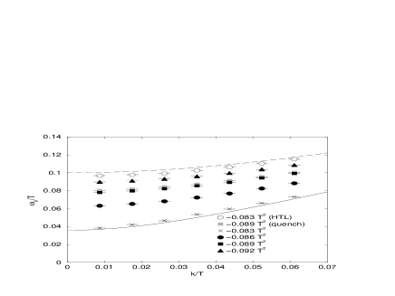
c)	d)

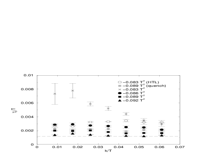
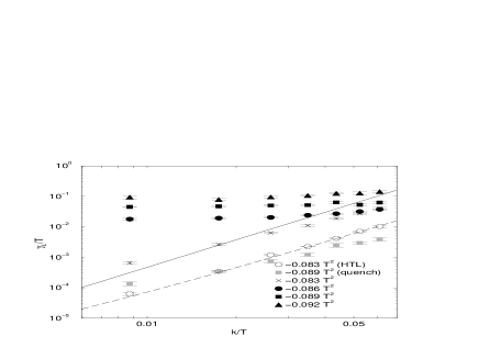
FIG. 2.: The real-time correlators measured at different values of $m^{2}$. a) Two examples of real-time correlators, measured at $m^{2}=-0.083T^{2}$ (solid) and $m^{2}=-0.086T^{2}$ (dashed), $k=0.026T$, together with fits of the form (30). b) The fitted plasmon frequencies $\omega_{p}$, and the perturbative estimates. c) The fitted plasmon damping rates $\gamma_{p}$. d) The fitted Landau damping rates $\gamma_{L}$, and the perturbative estimates. In plots b–d, the gray squares correspond to the state of the system after a quench and open circles to the HTL simulations discussed in Section V A.

The Landau damping rate in the symmetric phase has been calculated perturbatively in Ref. [25],

$$\gamma_{L}\approx\frac{7\delta x}{e^{2}T}k^{3}\approx 470\frac{k^{3}}{T^{2}}.$$ (33)

However, in our results the dependence on $\vec{k}$ is milder and we find the best fit with $\gamma_{L}\approx 15T^{-1.1}k^{2.1}$ above the transition point. Below the transition point, the exponential decay rate $\gamma_{L}$ becomes very large so that at late times, the correlator simply oscillates around zero (see Fig. 2a). In Fig. 2d, this behaviour can be seen in the values of the Landau damping rate.

In the defect formation scenario, the freeze-out occurs when Eq. (18) ceases to be satisfied. This happens most easily at the transition point, and there the real-time correlators are still the same as in the symmetric phase. Therefore, it is the symmetric phase correlators that determine the relevant time scale $\tau(k)$, and Fig. 2 shows clearly that for the long-wavelength modes, the lowest time scale is that of Landau damping, $\tau(k)\approx\gamma_{L}(k)^{-1}$.

Substituting $\tau(k)=\gamma_{L}(k)^{-1}$ to Eq. (18), we find

$$\frac{1}{\hat{k}^{2}}\frac{\delta m^{2}}{\tau_{Q}}\approx\gamma_{L}\approx 15T^{-1.1}\hat{k}^{2.1},$$ (34)

which implies

$$\hat{k}\approx\left(\frac{0.0061}{T\tau_{Q}}\right)^{1/4.1}T\approx 0.29T(T\tau_{Q})^{-0.24}\propto\tau_{Q}^{-0.24}.$$ (35)

B Phase transition

We simulated the phase transition by thermalizing a number of configurations with $m^{2}=m_{0}^{2}=-0.044T^{2}$, and solving numerically the equations of motion (23), varying the mass term with time according to

$$m^{2}(t)=m_{0}^{2}-\delta m^{2}\left(\frac{4}{3\pi}\arctan(t/\tau_{Q}-1)+\frac{1}{3}\right),$$ (36)

where $\delta m^{2}=0.089T^{2}$. This form of $m^{2}(t)$ has the advantage that long time after the transition, the system is in thermal equilibrium, making it possible to compare the final states.

The vortices produced in the transition are closed loops, and in general they will soon shrink to a point and disappear, which makes it very difficult to even define what we mean by the final vortex number. However, on a periodic lattice some of the vortex loops can be non-contractible, i.e. wind around the lattice in some direction. These loops can only disappear if they annihilate with another vortex of opposite direction, but this process is very slow, since the interactions between the vortices are exponentially suppressed at long distances. Therefore we chose one of the lattice dimensions much shorter than the other two (but still much longer than the microscopic length scales such as the Debye screening length $m_{D}^{-1}$.) A long time after the transition, when the system is deep in the broken phase, these vortices still remain and are well-defined macroscopic objects, and they can be counted without any ambiguities using the gauge-invariant lattice definition for the winding number [27, 28].

Because the scenario of defect formation discussed here is based on the assumption that the distribution of the magnetic field freezes in the transition, we can carry out a very simple test for the scenario by quenching the system through the transition and measuring the spatial correlator. We used $\tau_{Q}=300T^{-1}$ and stopped the quench at $m^{2}=-0.089T^{2}$ to carry out the measurement. The spatial correlator is shown in Fig. LABEL:fig:spatcorra as gray squares, and indeed, resembles much more the symmetric phase correlator than the equilibrium correlator at the same value of $m^{2}$. We also measured the real-time correlator, and the corresponding time scales are shown in Figs. 2b–c. The plasmon frequency and decay rate do not differ significantly from their equilibrium values, but Landau damping gets extremely slow. This means that once a mode has fallen out of equilibrium at the transition point, it takes a very long time before it thermalizes.

When one of the dimensions is shorter than $\hat{\xi}=2\pi/\hat{k}$, the prediction (20) changes into [4]

$$n\approx\frac{e}{2\pi}T^{1/2}L_{z}^{-1/2}\hat{k}^{-1}.$$ (37)

We tested this prediction by simulating the time evolution with different values of $\tau_{Q}$ and measuring the vortex number a long time after the transition at $t=\tau_{Q}+2400T^{-1}$. The results were published in Ref. [4], and are shown in Fig. 3. Each point is an average over around 15 runs starting from different initial configurations.

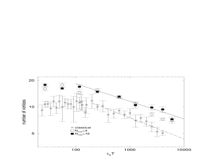
FIG. 3.: The dependence of the final number of vortices on the quench rate $\tau_{Q}$. The dashed line is a power-law fit of the data at $\tau_{Q}>200T^{-1}$ with the exponent $-0.24$ predicted by Eq. (35). The circles and squares correspond to the HTL simulations discussed in Section V B, and the solid line is a power-law fit of $\tau_{Q}>100T^{-1}$ using the exponent $-0.2$ predicted by Eq. (48).

Combining the result $\hat{k}\sim\tau_{Q}^{-0.24}$ from Eq. (35) with Eq. (37), we expect $N\approx c\tau_{Q}^{-0.24}$. If we determine the constant $c$ from the best fit to the data at $\tau_{Q}>200T^{-1}$, we find $c=39.5\pm 1.0$ and $\chi^{2}=7.6/13$ dof. This is shown in Fig. 3 as the dashed line. If we also leave the exponent as a free parameter, we find $N=(43.9\pm 7.9)(T\tau_{Q})^{-0.255\pm 0.026}$, with $\chi^{2}=7.2/12$ dof.

If we calculate precisely the prediction (37) using Eq. (35), we find $c\approx 650$ for the above fit parameter. However, it is not surprising that it differs from the measured value by a factor of $\approx 15$, not only because have we neglected factors or $2\pi$ and other numerical factors, but also because in our estimates we have assumed that the mechanism is ideally efficient and that all the magnetic flux is converted into vortices.

From the cosmological point of view, we are more interested in the area density of vortices in a fully three-dimensional case than in a thin box. Because the topology of the system does not prevent vortex loops from shrinking, the resulting network is not stable, unless it is stabilized by the expansion of the universe. We can therefore only use Eq. (20) as an estimate for the area density of vortices immediately after the transition. Comparing Eqs. (20) and (37), we find

$$n_{\rm 3D}=\left(\frac{2\pi}{e}\right)^{1/2}T^{-1/4}L_{z}^{3/4}n_{\rm 2D}^{3/2},$$ (38)

where $n_{\rm 2D}$ is given by Eq. (37) and $n_{\rm 3D}$ is the three-dimensional area density given by Eq. (20). In our case, $L_{z}=120T^{-1}$ and $A=5.2\times 10^{5}T^{-2}$, and we find

$$n_{\rm 3D}\approx 166T^{-1}n_{\rm 2D}^{3/2}\approx 1.3\times 10^{-4}(T\tau_{Q})^{-0.38}.$$ (39)

V HTL simulations

A Equilibrium

As discussed in Section II, the classical theory discussed above does not describe the dynamics of the quantum theory correctly. Therefore we also carried out the same simulations with the HTL improved theory (7). In the same way as in Section IV A, we first studied the equilibrium properties of the theory. We used the same couplings $e=0.3$ and $\lambda=0.18$ as in the classical case, and the same lattice. With these parameters, the Debye mass has the value $m^{2}_{D}=0.03T^{2}$. The number of Legendre modes was $N_{\rm max}=4$. The only effect of the HTL corrections to the thermodynamics is to give an extra contribution to electric screening, so we expect that the phase diagrams of the theories are practically the same. Therefore we only carried out the equilibrium measurements at the transition point, $m^{2}=-0.083T^{2}$.

Using the Hamiltonian (A24), we first prepared the thermal initial conditions with a Monte Carlo algorithm. This can be done in two steps:

1. Generate the soft mode configuration. The part of the Hamiltonian that involves the hard modes is Gaussian and therefore they can be integrated out exactly. This results in a theory with only the soft fields $\phi$ and $A_{i}$ and their canonical momenta. The Gauss law leads to an extra Debye screening term

   $$\delta H_{\rm Debye}=\frac{1}{2m_{D}^{2}}\left(\vec{\nabla}\cdot\vec{E}-2e{\rm Im}\phi^{*}\pi\right).$$ (40)

   in the Hamiltonian. We used a Metropolis algorithm for $\phi$ and a heat bath algorithm for all other fields, and carried out around 10000 thermalization sweeps.

2. Generate the hard modes in the background of the soft modes generated in step 1. Since the Hamiltonian is Gaussian it could in principle be diagonalized and the field values could be taken directly from a normal distribution. However, we did this only for $\theta$ and its momentum $\Pi$. Note that the lowest Legendre mode of $\Pi$ is fixed by the Gauss law,

   $$\Pi^{(0)}=-\frac{1}{m_{D}}\left(\vec{\nabla}\cdot\vec{E}-2e{\rm Im}\phi^{*}\pi\right).$$ (41)

   The field $\vec{f}$ and its momentum $\vec{F}$ were generated using a heat bath algorithm with around 5000 sweeps.

Again, we evolved the configurations taken from the thermal ensemble using the equations of motion (A17) for the time $\Delta t=12000T^{-1}$, measuring the equal-time and real-time correlators. The equal-time correlator is shown as open circles in Fig. LABEL:fig:spatcorr, and it agrees fairly well with the corresponding classical correlator. This time, the fit to the perturbative one-loop result (29) favours $M=0$, which suggests that because of the presence of the hard modes, the transition point is at slightly larger $m^{2}$ than in the classical case, and that $m^{2}=-0.083T^{2}$ is very close to it.

Because perturbation theory cannot be trusted at low momenta, we do not adopt the perturbative result (28), but instead we simply assume that the self energy is linear at small momenta

$$\Pi_{T}(k)=k_{\rm np}k,$$ (42)

and determine the coefficient $k_{\rm np}$ from the best fit to the data, which gives

$$k_{\rm np}=(0.0071\pm 0.0005)T,$$ (43)

and use this in our later estimates.

The hard modes have a significant effect on the real-time correlators, shown in Figs. 2b–d. Because they mimic the effect of the hard modes in the continuum quantum theory, we should now be able to compare the results with the standard perturbative calculations. For the plasmon mass, the perturbative result is [30, 21]

$$m_{p}=\frac{1}{\sqrt{3}}m_{D}=0.1T.$$ (44)

The dashed line in Fig. 2b shows the corresponding curve $\omega_{p}=\sqrt{k^{2}+m_{p}^{2}}$. The measured values are slightly below this curve, but the agreement is still very good.

The continuum plasmon damping rate at zero momentum has been computed perturbatively in the HTL approximation in Refs. [21, 24],

$$\gamma_{p}(T)=\frac{e^{2}T}{24\pi}A(T/T_{c},\lambda/e^{2}).$$ (45)

The function $A(T/T_{c},\lambda/e^{2})$ takes the value 1 at the critical point, peaks at value $\sim 1$ just below it, and vanishes above it when $m_{p}>2M$. In our case, the damping rate at the transition point would be

$$\gamma_{p}(T)\approx 0.0012T,$$ (46)

which is shown in Fig. 2c as a dashed line and is lower than value the measured at $m^{2}=-0.083T^{2}$ by roughly a factor of three. It has been observed earlier [26], that also in the SU(2) theory, the perturbative calculation underestimates the plasmon damping rate significantly. We can also note that the damping rate is lower than in the classical theory.

The Landau damping rate can be obtained directly from the HTL improved Lagrangian and is [30]

$$\gamma_{L}=\frac{4k^{2}}{\pi m_{D}^{2}}(k+k_{\rm np})\approx 42.4\frac{k^{2}}{T^{2}}(k+k_{\rm np}),$$ (47)

where we have taken into account the linear contribution (42) to the self energy. This curve is shown as the dashed line in Fig. 2d, and agrees well with the measured values. Again, we can conclude that the relevant time scale is that of Landau damping. If we can ignore the linear correction, we find [cf. Eq. (35)]

$$\hat{k}\approx\left(\frac{\pi}{4}m_{D}^{2}\frac{\delta m^{2}}{\tau_{Q}}\right)^{0.2}\approx 0.29T(T\tau_{Q})^{-0.2}\sim\tau_{Q}^{-0.2},$$ (48)

and in slowest transitions, we have

$$\hat{k}\approx\left(\frac{\pi}{4}\frac{m_{D}^{2}}{k_{\rm np}}\frac{\delta m^{2}}{\tau_{Q}}\right)^{0.25}\approx 0.74T(T\tau_{Q})^{-0.25}\sim\tau_{Q}^{-0.25}.$$ (49)

However, this corresponds to $\tau_{Q}\gg 10^{8}T^{-1}$, which is much larger than the values of $\tau_{Q}$ we are able to use in out simulations.

B Phase transition

As in Sect. IV B, we studied the non-equilibrium dynamics of the phase transition by starting from thermal configurations at $m^{2}=-0.044T^{2}$ and evolving the system with a time-dependent mass term (36). We used two different values for $N_{\rm max}$, $4$ and $16$.

In Fig. 3, we show how the final vortex number, measured at $t=2\tau_{Q}+2400T^{-1}$ depends on the quench rate $\tau_{Q}$. Each data point is an average over 20–30 runs. In fast transitions, $\tau_{Q}\mathop{\raise 1.29167pt\hbox{$<$\kern-7.5pt\raise-4.73611pt\hbox{$\sim$}}}1000T^{-1}$, the results for $N_{\rm max}=4$ and $16$ agree, but in slower transitions there is a statistically significant difference. This can be understood in terms of Eq. (10): For small $\tau_{Q}$, $N_{\rm max}=4$ is sufficient because by the time the approximation breaks down, the system is already so deep in the Higgs phase that the vortex number cannot change any more. When $\tau_{Q}$ gets larger, eventually a point is reached at which the breakdown occurs so early that it would have an effect on the final state. This may have happened even for $N_{\rm max}=16$ in the slowest transitions with $\tau_{Q}=6000T^{-1}$.

Combining Eq. (48) with Eq. (37), we find $N\sim\tau_{Q}^{-0.2}$. A fit to the $N_{\rm max}=16$ data at $\tau_{Q}>100T^{-1}$ with $N=c(T\tau_{Q})^{-0.2}$ gives $c=45.5\pm 0.9$ with $\chi^{2}=6.8/6$ dof, which shows that the results are compatible with the prediction. The fit is shown in Fig. 3 as a solid line. The prediction of Eq. (37) is $c\approx 660$, which is greater than the measured value by a factor of $\approx 15$. This is the same factor found in the classical case, which further supports our scenario. If we keep the exponent as a free parameter, we find $N=(45.9\pm 4.6)(T\tau_{Q})^{-0.201\pm 0.015}$, with $\chi^{2}=6.8/5$ dof.

Again, we relate the results to three dimensions using Eq. (38), and find

$$n_{\rm 3D}\approx 1.4\times 10^{-4}(\tau_{Q}T)^{-0.30}.$$ (50)

The conjectured non-perturbative behaviour at low momenta (42) would change this scaling law in very slow transitions. Eq. (20) would become $n\propto\hat{k}^{2}$, and Eq. (49) would therefore imply $n\propto\tau_{Q}^{-0.5}$.

VI Conclusions

In this paper we have presented a thorough study of the dynamics of the high temperature phase transition in the Abelian Higgs model, using both classical and HTL improved approximations. The aims were twofold. The first was to measure the equilibrium properties of the theory, and in particular find the relevant timescale for the decay of the long wavelength modes of the gauge field, which were identified in [4] as crucial to the understanding of vortex formation.

In Ref. [4], we performed numerical simulations of the Abelian Higgs model phase transition in real time by using the classical theory and changing the mass parameter of the Higgs field over a characteristic quench time $\tau_{Q}$. In this paper, our second aim was to do the same quenches with the HTL improved theory, and to compare the resulting scaling law for the number of vortices $N$ formed as a function of the quench time.

Our measurements of the equilibrium correlators show that perturbation theory gives a reasonable account of their behaviour, except perhaps for the plasmon damping rate. A new and unexpected result is that near the transition, the equal-time correlator exhibits power-law magnetic screening, with a coefficient that is similar but not equal to the perturbative one. In the HTL improved simulations, the numerical values of the plasmon mass and the Landau damping rate agree well with the perturbative values in the Coulomb phase. For the plasmon damping rate, however, the measured value was significantly higher than the perturbative estimate. As might be expected, the agreement is not as good in the classical theory: although the plasmon mass agrees well, the dependence of the Landau damping rate $\gamma_{L}$ on wavenumber $k$ is $\gamma_{L}\sim k^{2.1}$ rather than the expected $k^{3}$.

We found significant differences between the scaling laws for the classical simulations, and for HTL improved quenches with $N_{\rm max}=4$ and $N_{\rm max}=16$. The difference between the classical scaling law and the HTL improved one with $N_{\rm max}=16$ can be ascribed to the discrepancy in the Landau damping rate, and lends force to the contention made in [4] that it is the balancing of the cooling rate with the Landau damping rate which decides the length scale above which the fields fall out of equilibrium. The difference between $N_{\rm max}=4$ and $N_{\rm max}=16$ can be understood as stemming from a lack of phase space in the hard modes, which causes the HTL approximation to break down at times greater than $t_{c}(k)=4N_{\rm max}/k$.

Our simulations have been carried out to leading order in the couplings $e$ and $\lambda$, and hence do not include the effect of high momentum transfer scattering between the hard modes. However, the hard modes can still scatter by exchanging soft modes, we do not expect this to change the dynamics qualitatively on the relatively short time scales which we have been able to study. In very slow transitions, it may be that hard mode scattering and also non-perturbative effects in the photon self-energy start to become important and and the predicted scaling law $n\propto\tau_{Q}^{-0.3}$ ceases to be valid.

A HTL improved equations of motion

In Sect. II the local formulation of the HTL improved Abelian Higgs model was described. In this Appendix we detail the resulting equations of motion for the fields $\phi$ and $\vec{A}$ and Legendre modes $\theta$ and $\vec{f}$, which encode the effect of high momentum ($k\mathop{\raise 1.29167pt\hbox{$>$\kern-7.5pt\raise-4.73611pt\hbox{$\sim$}}}T$) particles.

These fields satisfy the equations of motion

$$\partial_{0}^{2}{\vec{A}} = -\vec{\nabla}\times\vec{\nabla}\times\vec{A}-2e{\rm Im}\phi^{*}\vec{D}\phi$$ (A2)

$$+m_{D}\int_{0}^{1}dzz^{2}\left(\vec{\nabla}\theta-m_{D}\vec{A}+\sqrt{\frac{1-z^{2}}{2z^{2}}}\vec{\nabla}\times\vec{f}\right),$$

$$\partial_{0}^{2}{\vec{f}}(z) = -z^{2}\vec{\nabla}\times\vec{\nabla}\times\vec{f}+m_{D}z\sqrt{\frac{1-z^{2}}{2}}\vec{\nabla}\times\vec{A},$$ (A3)

$$\partial_{0}^{2}{\theta}(z) = z^{2}\vec{\nabla}\cdot\left(\vec{\nabla}\theta-m_{D}\vec{A}\right).$$ (A4)

Since these equations for $\vec{f}$ and $\theta$ are linear, it is easy to solve them and show that the dynamics of $\phi$ and $A_{i}$ is identical to the original non-local theory (9).

Not only is this reformulation of the theory local, but the equations of motion are in a canonical form and we can therefore write down the corresponding Hamiltonian

$$H = \int d^{3}x\int_{0}^{1}dz\Biggl{[}\frac{1}{2}\vec{E}^{2}+\frac{1}{2}(\vec{\nabla}\times\vec{A})^{2}+\pi^{*}\pi+(D_{i}\phi)^{*}(D_{i}\phi)+m_{T}^{2}\phi^{*}\phi+\lambda(\phi^{*}\phi)^{2}$$ (A6)

$$+\frac{1}{2}\vec{F}^{2}+\frac{1}{2}{\Pi}^{2}+\frac{z^{2}}{2}(\vec{\nabla}\times\vec{f})^{2}+\frac{z^{2}}{2}(\vec{\nabla}\theta-m_{D}\vec{A})^{2}-m_{D}z\sqrt{\frac{1-z^{2}}{2}}\vec{f}\cdot\vec{\nabla}\times\vec{A}\Biggr{]},$$

where $\vec{F}=\partial_{0}{\vec{f}}$ and $\Pi=\partial_{0}\theta$ are the canonical momenta of $\vec{f}$ and $\theta$, respectively. We also need two extra conditions, namely the transverseness of $\vec{f}$ and Gauss’s law

$$\vec{\nabla}\cdot\vec{f} = \vec{\nabla}\cdot\vec{F}=0,$$ (A7)

$$\vec{\nabla}\cdot\vec{E} = -m_{D}\int_{0}^{1}dz\Pi(z)+2e{\rm Im}\phi^{*}\pi.$$ (A8)

The $z$ dependence of $\vec{f}$ and $\theta$ is discretized [10] by introducing the Legendre modes

$$\vec{f}^{(n)} = \int_{0}^{1}dzz\sqrt{\frac{2}{1-z^{2}}}P_{2n}(z)\vec{f}(z),\quad\theta^{(n)}=\int_{0}^{1}dzP_{2n}(z)\theta(z),$$ (A9)

$$\vec{F}^{(n)} = \int_{0}^{1}\frac{dz}{z}\sqrt{\frac{2}{1-z^{2}}}P_{2n}(z)\vec{F}(z),\quad\Pi^{(n)}=\int_{0}^{1}dzP_{2n}(z)\Pi(z).$$ (A10)

Note that we have used slightly different definitions from Ref. [10], in order to write the Hamiltonian in a practical form.

In terms of these modes, the equations of motion become

$$\partial_{0}\vec{A} = -\vec{E},$$ (A11)

$$\partial_{0}{\vec{f}}^{(n)} = C^{+}_{n}\vec{F}^{(n+1)}+C^{0}_{n}\vec{F}^{(n)}+C^{-}_{n}\vec{F}^{(n-1)},$$ (A12)

$$\partial_{0}{\theta}^{(n)} = \Pi^{(n)},$$ (A13)

$$\partial_{0}{\vec{E}} = \vec{\nabla}\times\vec{\nabla}\times\vec{A}+2e{\rm Im}\phi^{*}\vec{D}\phi+\frac{1}{3}m_{D}^{2}\vec{A}$$ (A15)

$$-\frac{1}{3}m_{D}\left(\vec{\nabla}\theta^{(0)}+2\vec{\nabla}\theta^{(1)}+\vec{\nabla}\times\vec{f}^{(0)}-\vec{\nabla}\times\vec{f}^{(1)}\right),$$

$$\partial_{0}\vec{F}^{(n)} = -\vec{\nabla}\times\vec{\nabla}\times\vec{f}^{(n)}+m_{D}\vec{\nabla}\times\vec{A}\delta_{n,0},$$ (A16)

$$\partial_{0}\Pi^{(n)} = C^{+}_{n}\vec{\nabla}^{2}\theta^{(n+1)}+C^{0}_{n}\vec{\nabla}^{2}\theta^{(n)}+C^{-}_{n}\vec{\nabla}^{2}\theta^{(n-1)}-m_{D}\vec{\nabla}\cdot\vec{A}\left(\frac{1}{3}\delta_{n,0}+\frac{2}{15}\delta_{n,1}\right),$$ (A17)

where

$$C^{+}_{n}=\frac{(2n+1)(2n+2)}{(4n+1)(4n+3)},\quad C^{0}_{n}=\frac{1}{4n+1}\left(\frac{(2n+1)^{2}}{4n+3}+\frac{4n^{2}}{4n-1}\right),\quad C^{-}_{n}=\frac{2n(2n-1)}{(4n+1)(4n-1)}.$$ (A18)

The Hamiltonian becomes

$$H = \int d^{3}x\Biggl{\{}\frac{1}{2}\vec{E}^{2}+\frac{1}{2}(\vec{\nabla}\times\vec{A})^{2}+\pi^{*}\pi+(D_{i}\phi)^{*}(D_{i}\phi)+m_{T}^{2}\phi^{*}\phi+\lambda(\phi^{*}\phi)^{2}$$ (A24)

$$+\sum_{n=0}^{\infty}\left[\frac{1}{4}\frac{1}{4n+3}\left((2n+1)\vec{F}^{(n)}+(2n+2)\vec{F}^{(n+1)}\right)^{2}\right.$$

$$-\frac{4n+1}{4}\left(C^{+}_{n}\vec{F}^{(n+1)}+C^{0}_{n}\vec{F}^{(n)}+C^{-}_{n}\vec{F}^{(n-1)}\right)^{2}$$

$$+\frac{4n+1}{4}\left(\vec{\nabla}\times\vec{f}^{(n)}\right)^{2}-\frac{1}{4}\frac{1}{4n+3}\left((2n+1)\vec{\nabla}\times\vec{f}^{(n)}+(2n+2)\vec{\nabla}\times\vec{f}^{(n+1)}\right)^{2}$$

$$+\frac{4n+1}{2}\left(\Pi^{(n)}\right)^{2}+\frac{1}{2}\frac{1}{4n+3}\left((2n+1)\vec{\nabla}\theta^{(n)}+(2n+2)\vec{\nabla}\theta^{(n+1)}\right)^{2}$$

$$\left.+\frac{m_{D}}{3}\vec{\nabla}\cdot\vec{A}\left(\theta^{(0)}+2\theta^{(1)}\right)-\frac{m_{D}}{3}\vec{\nabla}\times\vec{A}\left(\vec{f}^{(0)}-\vec{f}^{(1)}\right)+\frac{1}{6}m_{D}^{2}\vec{A}^{2}\right]\Biggr{\}},$$

B Lattice discretization

1 Classical theory

In order to carry out numerical simulations described in Section IV, we discretize the Hamiltonian (21) and the equations of motion (23) in the standard leap-frog fashion. The Higgs field $\phi$ was defined at the lattice sites, and its canonical momentum at temporal links between time slices. The gauge field $\vec{A}$ was represented by real numbers defined at links between lattice sites, and the electric field $\vec{E}$ by temporal plaquettes that connect these links. Therefore $\pi_{(t,\vec{x})}$ is actually defined at the point $(t+\delta t/2,\vec{x})$, $A_{i,(t,\vec{x})}$ at $(t,\vec{x}+\hat{\imath}/2)$ and $E_{i,(t,\vec{x})}$ at $(t+\delta t/2,\vec{x}+\hat{\imath}/2)$. Here $\hat{\imath}$ is a vector of length $\delta x$ in the $i$ direction.

The lattice version of the Hamiltonian (21) is

$$H = \sum_{\vec{x}}\delta x^{3}\left[\frac{1}{2}\sum_{i}E_{i}+\frac{1}{2}\sum_{i}\left(\epsilon_{ijk}\Delta_{j}^{+}A_{k}\right)^{2}+\pi^{*}\pi\right.$$ (B2)

$$\left.-\frac{2}{\delta x^{2}}\sum_{i}{\rm Re}\phi_{(\vec{x})}^{*}U_{i,(\vec{x})}\phi_{(\vec{x}+\hat{\imath})}+\left(m_{T}^{2}+\frac{6}{\delta x^{2}}\right)|\phi|^{2}+\lambda|\phi|^{4}\right].$$

where

$$U_{i} = \exp\left(ie\delta xA_{i}\right),$$ (B3)

$$\Delta^{\pm}_{i}\phi_{(\vec{x})} = \pm\delta x^{-1}\left(\phi_{(\vec{x}\pm\hat{\imath})}-\phi_{(\vec{x})}\right).$$ (B4)

We also define the lattice version of the covariant derivative

$$D^{+}_{i}\phi_{(\vec{x})} = \delta x^{-1}\left(U_{i,(\vec{x})}\phi_{(\vec{x}+\hat{\imath})}-\phi_{(\vec{x})}\right),$$ (B5)

$$D^{-}_{i}\phi_{(\vec{x})} = \delta x^{-1}\left(\phi_{(\vec{x})}-U^{*}_{i,(\vec{x}-\hat{\imath})}\phi_{(\vec{x}-\hat{\imath})}\right).$$ (B6)

The value of the bare lattice mass $m^{2}_{T}$ is given by Eq. (3) and was chosen in such a way that the Hamiltonian (B2) describes the thermodynamics of the finite-temperature theory with renormalized mass $m^{2}$ correctly [18, 19].

The discretized equations of motion are

$$\Delta_{t}E_{i,(t,\vec{x})} = \epsilon_{ijk}\epsilon_{klm}\Delta^{-}_{j}\Delta^{+}_{l}A_{i,(t,\vec{x})}-2e{\rm Im}\phi^{*}_{(t,\vec{x})}D^{+}_{i}\phi_{(t,\vec{x})},$$ (B7)

$$\Delta_{t}\pi_{(t,\vec{x})} = D_{i}^{-}D_{i}^{+}\phi_{(t,\vec{x})}-m_{T}^{2}\phi_{(t,\vec{x})}-2\lambda|\phi_{(t,\vec{x})}|^{2}\phi_{(t,\vec{x})},$$ (B8)

$$\Delta_{t}A_{i,(t+\delta t,\vec{x})} = -E_{i,(t,\vec{x})},$$ (B9)

$$\Delta\phi_{(t+\delta t,\vec{x})} = \pi_{(t,\vec{x})},$$ (B10)

where $\Delta_{t}\phi_{(t)}=\delta t^{-1}[\phi_{(t)}-\phi_{(t-\delta t)}]$ etc.

The lattice version of the Gauss law (22) is

$$\sum_{i}\Delta^{-}_{i}E_{i,(t,\vec{x})}=2e{\rm Im}\phi^{*}_{(t,\vec{x})}\pi_{(t,\vec{x})}.$$ (B11)

This is an extra constraint the initial field configuration must satisfy.

2 HTL theory

In the HTL simulations described in Section V, the soft modes were discretized in the same way as in the classical case. The extra field $\theta$ is defined at lattice sites and $f_{i}$ at the plaquettes. We denote by $f_{i,(t,\vec{x})}$ the field value at $(t,\vec{x}+\hat{x}/2+\hat{y}/2+\hat{z}/2-\hat{\imath}/2)$.

The lattice version of the HTL-improved Hamiltonian (A24) is

$$H_{\rm HTL}=H+\delta x^{3}\sum_{\vec{x}}\left[{\cal H}_{F}+{\cal H}_{f}+{\cal H}_{\Pi}+{\cal H}_{\theta}\right],$$ (B12)

where

$${\cal H}_{F} = \sum_{n=0}^{\infty}\frac{1}{4}\left[\frac{1}{4n+3}\left((2n+1)\vec{F}^{(n)}+(2n+2)\vec{F}^{(n+1)}\right)^{2}\right.$$ (B14)

$$\left.-(4n+1)\left(C^{+}_{n}\vec{F}^{(n+1)}+C^{0}_{n}\vec{F}^{(n)}+C^{-}_{n}\vec{F}^{(n-1)}\right)^{2}\right],$$

$${\cal H}_{f} = \sum_{n=0}^{\infty}\left[\frac{4n+1}{4}\left(\epsilon_{ijk}\Delta^{-}_{j}f_{k}^{(n)}\right)^{2}-\frac{1}{4}\frac{1}{4n+3}\left((2n+1)\epsilon_{ijk}\Delta^{-}_{j}f_{k}^{(n)}\right.\right.$$ (B16)

$$\left.\left.+(2n+2)\epsilon_{ijk}\Delta^{-}_{j}f_{k}^{(n+1)}\right)^{2}\right]-\frac{m_{D}}{3}\epsilon_{ijk}\Delta_{j}^{+}A_{k}\left(f_{k}^{(0)}-f_{k}^{(1)}\right)+\frac{1}{6}m_{D}^{2}A_{i}^{2},$$

$${\cal H}_{\Pi} = \sum_{n=0}^{\infty}\frac{4n+1}{2}\left(\Pi^{(n)}\right)^{2},$$ (B17)

$${\cal H}_{\theta} = \sum_{n=0}^{\infty}\frac{1}{2}\frac{1}{4n+3}\left((2n+1)\Delta^{+}_{i}\theta^{(n)}+(2n+2)\Delta^{+}_{i}\theta^{(n+1)}\right)^{2}+\frac{m_{D}}{3}\Delta^{-}_{i}A_{i}\left(\theta^{(0)}+2\theta^{(1)}\right).$$ (B18)

The Gauss law (A8) can be written in the form

$$\Pi^{(0)}_{(t,\vec{x})}=\frac{1}{m_{D}}\left(\sum_{i}\Delta^{-}_{i}E_{i,(t,\vec{x})}-2e{\rm Im}\phi^{*}_{(t,\vec{x})}\pi_{(t,\vec{x})}\right),$$ (B19)

and therefore we can eliminate $\Pi^{(0)}$ from the Hamiltonian.

The bare Higgs mass has the value given in Eq. (3), and the Debye mass is [18, 19]

$$m_{D}^{2}=\frac{1}{3}e^{2}T^{2}-2e^{2}\frac{3.176T}{4\pi\delta x}.$$ (B20)

These counterterms were calculated by matching static correlators and in the absence of Lorenz invariance, they do not remove all the ultraviolet divergences from real-time quantities. However, since our lattice spacing is relatively large, this leads only to small errors.

The discretized equations of motion are

$$\Delta_{t}E_{i,(t,\vec{x})} = \epsilon_{ijk}\epsilon_{klm}\Delta^{-}_{j}\Delta^{+}_{l}A_{i,(t,\vec{x})}-2e{\rm Im}\phi^{*}_{(t,\vec{x})}D^{+}\phi_{i,(t,\vec{x})}$$ (B22)

$$-\frac{m_{D}}{3}\left(\Delta^{+}_{i}\theta^{(0)}_{(t,\vec{x})}+2\Delta^{+}_{i}\theta^{(1)}_{(t,\vec{x})}+\epsilon_{ijk}\Delta^{-}_{j}f^{(0)}_{k,(t,\vec{x})}-\epsilon_{ijk}\Delta^{-}_{j}f^{(1)}_{k,(t,\vec{x})}\right),$$

$$\Delta_{t}\pi_{(t,\vec{x})} = D_{i}^{-}D_{i}^{+}\phi_{(t,\vec{x})}-m_{T}^{2}\phi_{(t,\vec{x})}-2\lambda|\phi_{(t,\vec{x})}|^{2}\phi_{(t,\vec{x})},$$ (B23)

$$\Delta_{t}F_{i,(t,\vec{x})}^{(n)} = -\epsilon_{ijk}\epsilon_{klm}\Delta^{+}_{j}\Delta^{-}_{l}f_{m,(t,\vec{x})}^{(n)}+\delta_{n,0}m_{D}\epsilon_{ijk}\Delta^{+}_{j}A_{k,(t,\vec{x})},$$ (B24)

$$\Delta_{t}\Pi_{(t,\vec{x})}^{(n)} = C^{+}_{n}\Delta_{i}^{+}\Delta_{i}^{-}\theta^{(n+1)}_{(t,\vec{x})}+C^{0}_{n}\Delta_{i}^{+}\Delta_{i}^{-}\theta^{(n)}_{(t,\vec{x})}+C^{-}_{n}\Delta_{i}^{+}\Delta_{i}^{-}\theta^{(n-1)}_{(t,\vec{x})}$$ (B26)

$$-m_{D}\Delta_{i}^{-}A_{i,(t,\vec{x})}\left(\frac{1}{3}\delta_{n,0}+\frac{2}{15}\delta_{n,1}\right),$$

$$\Delta_{t}A_{i,(t+\delta t,\vec{x})} = -E_{i,(t,\vec{x})},$$ (B27)

$$\Delta_{t}\phi_{(t+\delta t,\vec{x})} = \pi_{(t,\vec{x})},$$ (B28)

$$\Delta_{t}f_{i,(t+\delta t,\vec{x})}^{(n)} = C^{+}_{n}F_{i,(t,\vec{x})}^{(n+1)}+C^{0}_{n}F_{i,(t,\vec{x})}^{(n)}+C^{-}_{n}F_{i,(t,\vec{x})}^{(n-1)},$$ (B29)

$$\Delta_{t}\theta_{(t+\delta t,\vec{x})}^{(n)} = \Pi_{(t,\vec{x})}^{(n)}.$$ (B30)

REFERENCES

- [1] T. W. Kibble, J. Phys. A A9, 1387 (1976).
- [2] M. B. Hindmarsh and T. W. Kibble, Rept. Prog. Phys. 58, 477 (1995) [hep-ph/9411342].
- [3] W. H. Zurek, Phys. Rept. 276, 177 (1996) [cond-mat/9607135].
- [4] M. Hindmarsh and A. Rajantie, Phys. Rev. Lett. 85, 4660 (2000) [cond-mat/0007361]; A. Rajantie, cond-mat/0102403.
- [5] D. Y. Grigoriev and V. A. Rubakov, Nucl. Phys. B299, 67 (1988).
- [6] R. D. Pisarski, Phys. Rev. Lett. 63, 1129 (1989).
- [7] E. Braaten and R. D. Pisarski, Phys. Rev. D45, 1827 (1992).
- [8] J. P. Blaizot and E. Iancu, Phys. Rev. Lett. 70, 3376 (1993) [hep-ph/9301236].
- [9] G. D. Moore, C. Hu and B. Muller, Phys. Rev. D 58, 045001 (1998) [hep-ph/9710436].
- [10] A. Rajantie and M. Hindmarsh, Phys. Rev. D60, 096001 (1999) [hep-ph/9904270].
- [11] H. B. Nielsen and P. Olesen, Nucl. Phys. B61, 45 (1973).
- [12] A. D. Linde, Phys. Lett. B96, 289 (1980).
- [13] P. Dimopoulos, K. Farakos and G. Koutsoumbas, Eur. Phys. J. C1, 711 (1998) [hep-lat/9703004].
- [14] K. Kajantie, M. Karjalainen, M. Laine and J. Peisa, Nucl. Phys. B520, 345 (1998) [hep-lat/9711048].
- [15] K. Kajantie, M. Laine, T. Neuhaus, J. Peisa, A. Rajantie and K. Rummukainen, Nucl. Phys. B546, 351 (1999) [hep-ph/9809334].
- [16] K. Kajantie, M. Laine, K. Rummukainen and M. Shaposhnikov, Nucl. Phys. B493, 413 (1997) [hep-lat/9612006].
- [17] A. J. Niemi and G. W. Semenoff, Annals Phys. 152, 105 (1984).
- [18] M. Laine, Nucl. Phys. B451, 484 (1995) [hep-lat/9504001].
- [19] M. Laine and A. Rajantie, Nucl. Phys. B513, 471 (1998) [hep-lat/9705003].
- [20] D. Bödeker, L. McLerran and A. Smilga, Phys. Rev. D52, 4675 (1995) [hep-th/9504123].
- [21] U. Kraemmer, A. K. Rebhan and H. Schulz, Annals Phys. 238, 286 (1995) [hep-ph/9403301].
- [22] W. H. Zurek, Acta Phys. Polon. B24, 1301 (1993).
- [23] J. Blaizot, E. Iancu and R. R. Parwani, Phys. Rev. D 52, 2543 (1995) [hep-ph/9504408].
- [24] T. S. Evans and A. C. Pearson, Phys. Rev. D 55, 3748 (1997) [hep-ph/9502209].
- [25] P. Arnold, Phys. Rev. D55, 7781 (1997) [hep-ph/9701393].
- [26] D. Bödeker and M. Laine, Phys. Lett. B 416, 169 (1998) [hep-ph/9707489].
- [27] J. Ranft, J. Kripfganz and G. Ranft, Phys. Rev. D28, 360 (1983).
- [28] K. Kajantie, M. Karjalainen, M. Laine, J. Peisa and A. Rajantie, Phys. Lett. B428, 334 (1998) [hep-ph/9803367].
- [29] P. Ginsparg, Nucl. Phys. B170, 388 (1980).
- [30] E. M. Lifshitz and L. P. Pitaevskii, Physical Kinetics, Landau and Lifshitz Course of Theoretical Physics Volume 10, (Pergamon Press, Oxford, 1981).