Abstract

In this talk some of the theoretical aspects of $b\to s\gamma$ transitions are discussed. The focus is on inclusive decays, since these can be computed more reliably. Topics covered are (1) perturbative QCD corrections, (2) non-perturbative contributions and (3) effects of “new physics” in these decays.

1 Introduction

Radiative rare $B$ decays have attracted considerable attention in the last few years. After the first observation in 1994, by the CLEO collaboration [1], data have become quite precise [2] so that even a measurement of the CP asymmetry in these decays [3, 4] became possible. As far as data are concerned, the situation clearly will improve further, after the excellent start of both $B$ factories at KEK and at SLAC.

$B\to X_{s}\gamma$ tests the Standard Model (SM) in a particular way. Since there are no tree-level contributions to these processes in the SM, they can occur only at the one-loop level. The GIM cancellation, which is present in all the FCNC processes, is lifted in this case by the large top-quark mass; if the top quark were as light as the $b$ quark, these decays would be too rare to be observable.

Since the SM contribution is small, these decays have a good sensitivity to “new physics”, e.g. to new (heavy) particles contributing to the loop. In fact, already the first CLEO data could constrain some models for “new physics” in a stringent way[1].

The most general effective Hamiltonian describing these decays is given by

$$H_{eff}=\sum_{i}c_{i}\,O_{i}\,,$$ (1)

where the $O_{i}$ are local operators

$$O_{1\cdots 6} =$$ four-fermion operators

$$O_{7} = m_{b}\bar{s}\sigma_{\mu\nu}(1+\gamma_{5})b\,F^{\mu\nu}$$

$$O_{7}^{\prime} = m_{s}\bar{s}\sigma_{\mu\nu}(1-\gamma_{5})b\,F^{\mu\nu}$$

$$O_{8} = m_{b}\bar{s}\sigma^{\mu\nu}T^{a}(1+\gamma_{5})b\,G_{\mu\nu}^{a}$$

$$O_{8}^{\prime} = m_{s}\bar{s}\sigma^{\mu\nu}T^{a}(1-\gamma_{5})b\,G_{\mu\nu}^{a}$$ (2)

and $c_{i}$ are pertubatively calculable coefficients.

In any new physics analysis of $B$ decays only the coefficients $c_{i}$ are tested [5]. The decay $B\to X_{s}\gamma$ (and the corresponding exclusive decays) are practically determined by the two operators $O_{7}$ and $O_{7}^{\prime}$, and hence these decays are mainly testing $c_{7}$ and $c_{7}^{\prime}$. In the SM these two coefficients are

$$c_{7}=-\frac{G_{F}^{2}e}{32\sqrt{2}\pi^{2}}V_{tb}V_{ts}^{*}C_{7}m_{b},$$ (3)

$$c_{7}^{\prime}=-\frac{G_{F}^{2}e}{32\sqrt{2}\pi^{2}}V_{tb}V_{ts}^{*}C_{7}m_{s}$$ (4)

where $C_{7}$ is a function of $(m_{t}/M_{W})^{2}$, which we shall discuss later.

Furthermore, the two operators differ by the handedness of the quarks; in order to disentangle these two contributions there has to be a handle on the polarization of the quarks or of the photon, which is impossile at a $B$ factory. Consequently, from $b\to s\gamma$ alone only the combination $|c_{7}|^{2}+|c_{7}^{\prime}|^{2}$ can be determined in the near future.

Once the effective interaction for the quark transition is fixed, one has to calculate from this the actual hadronic process. This step is only for the inclusive decays under reasonable theoretical control; for exclusive decays, form factors are needed, which either need to be modelled or will finally come from the lattice.

For inclusive decays the machinery used is the heavy mass expansion. Using this framework for the total rate one can establish that (1) the leading term as $m_{b}\to\infty$ is the free quark decay, (2) there are no subleading corrections of order $1/m_{b}$, (2) the first non-vanising corrections are of order $1/m_{b}^{2}$ and are given in terms of two parameters. This will be discussed in section 3. Additional non-perturbative uncertainties are induced by a cut on the photon energy, which is necessary from the exprimental point of view to suppress backgrounds.

Part I deals with the perturbative corrections, part II with the non-perturbative ones. In part III, “new physics” in $b\to s\gamma$ is considered.

2 PART I: Perturbative Corrections

The main perturbative corrections are the QCD corrections, which are substantial. These corrections are calculated using an effective field-theory framework. To set this up, we have to write down first the relevant effective Hamiltonian as in (1). The operators appearing in (1) mix under renormalization as we evolve down from the $M_{W}$ mass scale to the relevant scale, which is the mass of the $b$ quark. The cofficient functions are calculated at the scale $\mu=M_{W}$ as a power series in the strong coupling

$$c_{i}(M_{W})=c_{i}^{(0)}(M_{W})+\frac{\alpha_{s}(M_{W})}{\pi}c_{i}^{(1)}(M_{W})+\cdots$$ (5)

Changing the scale $\mu$ results in a change of the coefficient functions and in the matrix elements, such that the matrix element of the effective Hamiltonian remains $\mu$-independent. This change can be computed perturbatively for sufficiently large $\mu$, using the standard machinery of renormalization group, which involves a calculation of the anomalous-dimension matrix that describes the mixing of the operators (1).

The solution of the renormalizaton group equation yields the coefficient functions at some lower scale $\mu$, which take the form (schematically)

$$c_{i}(\mu)=c_{i}^{(0)}(M_{W})\sum_{n=0}b_{n}^{(0)}\left(\frac{\alpha_{s}}{\pi}\ln\left(\frac{M_{W}^{2}}{\mu^{2}}\right)\right)^{n}$$ (6)

$$\quad+\frac{\alpha_{s}}{\pi}c_{i}^{(1)}(M_{W})\sum_{n=0}b_{n}^{(1)}\left(\frac{\alpha_{s}}{\pi}\ln\left(\frac{M_{W}^{2}}{\mu^{2}}\right)\right)^{n}+\cdots$$

where the $b_{n}$ are obtained from the solution of the renormalization group equation.

The last step is to compute the matrix elements of the operators at a scale $\mu\approx m_{b}$. This can be done for the inclusive case using the $1/m_{b}$ expansion. For the exclusive case, one would need the form factor in the corresponding approximation, which cannot be done with present theoretical techniques.

At present, the leading and the subleading terms of the coefficients have been calculated [11, 12, 13, 14], including electroweak contributions[15], the main part of which is due to the correct scale setting in $\alpha_{em}$.

A complete and up-to-date compilation can be found in [16]. Without going into any more detail we only quote the result from [16]

$$Br(B\to X_{s}\gamma)=(3.29\pm 0.33)\times 10^{-4}\,.$$ (7)

where this result includes a cut on the photon energy at $E_{\gamma,min}=0.05\,m_{b}$.

The QCD corrections are in fact dramatic; they increase the rate for $b\to s\gamma$ by about a factor of two. For example, already at the leading-log level we have $c_{7}(m_{b})/c_{7}(M_{W})=1.63$. Another indication of this fact is a substantial dependence of the leading-order result on the choice of the renormalization scale $\mu$. This is usually estimated by varying the scale $\mu$ between $m_{b}/2$ and $2m_{b}$. In this way one obtains a variation of $\delta_{\mu}={}^{+27.4\%}_{-20.4\%}$ for the leading-order result.

Taking into account the subleading terms reduces the scale dependence substantially. In fact, one has at subleading order [16] $\delta_{\mu}={}^{+0.1\%}_{-3.2\%}$, which is smaller than naively expected [17]. It has been argued that the smallness of $\delta_{\mu}$ is accidental [16]. However, arguments have been given recently [18] that these cancellations are not accidental. In fact, most of the large radiative corrections may be assigned to the running of the $b$ quark mass appearing in the operator $O_{7}$.

3 PART II: Non-Perturbative Corrections

Non-perturbative corrections arise from different sources. We shall consider here

• Long-distance effects from intermediate vector mesons $B\to J/\Psi X_{s}\to X_{s}\gamma$,

• Subleading terms in the heavy mass expansion: $1/m_{b}$ and $1/m_{c}$ corrections,

• Non-perturbative contributions to the photon spectrum (“shape function”).

3.1 $B\to J/\Psi X_{s}\to X_{s}\gamma$

One long-distance contribution comes from the process $B\to X_{s}J/\Psi$ and the subsequent decay of the (off-shell) $J/\Psi$ into a photon. The first process $B\to X_{s}J/\Psi$ has a branching ratio of order 1%, at least for an on-shell $J/\Psi$. Assuming that this is similar for the off-shell case, we have to multiply it with another factor $1/m_{c}^{2}$ for the propagation of the $J/\Psi$ and a factor $f_{J/\Psi}^{2}$, since the $J/\Psi$ has to annihilate into a photon. This leads us to the conclusion that this contribution is indeed negligibly small. However, one has to keep in mind that some extrapolation from $q^{2}=m_{J/\Psi}^{2}$ to $q^{2}=0$ is involved, assuming that this will not lead to a strong enhancement.

3.2 $1/m_{b}$ and $1/m_{c}$ corrections

A set of “standard” non-perturbative corrections arises from the heavy mass expansion [6, 7, 8, 9, 10]. As far as the total rate is concerned, we have the subleading corrections of order $1/m_{b}^{2}$, which are parametrized in terms of the kinetic energy $\lambda_{1}$ and the chromomagnetic moment $\lambda_{2}$ defined by the matrix elements

$$2M_{H}\lambda_{1} = \langle H(v)|\bar{h}_{v}(iD)^{2}h_{v}|H(v)\rangle$$ (8)

$$6M_{H}\lambda_{2} = \langle H(v)|\bar{h}_{v}\sigma_{\mu\nu}iD^{\mu}iD^{\nu}h_{v}|H(v)\rangle\,.$$ (9)

In terms of these two matrix elements the total rate reads at tree level up to order $1/m_{b}^{2}$

$$\Gamma=\frac{G_{F}^{2}\alpha m_{b}^{5}}{32\pi^{4}}|V_{ts}V_{tb^{*}}|^{2}|C_{7}|^{2}\left(1+\frac{\lambda_{1}-9\lambda_{2}}{2m_{b}^{2}}+\cdots\right)\,.$$ (10)

This result is fully integrated over the photon energy spectrum. One can also compute the energy spectrum of the photon within the $1/m_{b}$ expansion, which is given, again at tree level, by

$$\frac{d\Gamma}{dx}=\frac{G_{F}^{2}\alpha m_{b}^{5}}{32\pi^{4}}|V_{ts}V_{tb^{*}}|^{2}|C_{7}|^{2}$$ (11)

$$\left(\delta(1-x)-\frac{\lambda_{1}+3\lambda_{2}}{2m_{b}^{2}}\delta^{\prime}(1-x)+\frac{\lambda_{1}}{6m_{b}^{2}}\delta^{\prime\prime}(1-x)+\cdots\right)$$

which can only be interpreted in terms of moments of the spectrum. We shall return to this point in the next subsection.

Figure 1: Interference between $O_{7}$ and one of the four-fermion operators ($O_{2}$), leading to a contribution of order $1/m_{c}^{2}$

If the charm quark is also assumed to be heavy, one may discuss the charm-mass dependence in terms of a $1/m_{c}$ expansion [19]. The relevant contribution originates from the four-fermion operators (e.g. the operator $O_{2}$) involving the charm quark, see fig. 1. Expanding the matrix element of $O_{2}$ in powers of $1/m_{c}$ we obtain a local operator of the form

$$O_{1/m_{c}^{2}}=\frac{1}{m_{c}^{2}}\bar{s}\gamma_{\mu}(1-\gamma_{5})T^{a}b\,G^{a}_{\nu\lambda}\epsilon^{\mu\nu\rho\sigma}\partial^{\lambda}F_{\rho\sigma}$$ (12)

which can interfere with the leading term $O_{7}$ (see fig. 1).

The detailed calculation [20, 21] reveals that this contribution is rather small

$$\frac{\delta\Gamma_{1/m_{c}^{2}}}{\Gamma}=-\frac{C_{2}}{9C_{7}}\frac{\lambda_{2}}{m_{c}^{2}}\approx 0.03$$ (13)

3.3 Non-perturbative corrections in the photon energy spectrum

The non-perturbative corrections for the total rate are thus quite small and can safely be neglected against the perturbative ones. However, to extract the process $B\to X_{s}\gamma$ there has to be a lower cut on the photon energy to get rid of the uninteresting processes such as ordinary bremsstrahlung. Clearly it is desirable to have this cut as high as possible, but this makes the process “less inclusive” and hence more sensitive to non-perturbative contributions to the photon-energy spectrum.

Since we are dealing at tree level with a two-body decay, the naive calculation of the photon spectrum yields a $\delta$ function at partonic level and the $1/m_{b}^{n}$ corrections are again distributions located at the partonic energy $E_{\gamma}=m_{b}/2$, see (11). Clearly (11) cannot be used to implement a cut on the photon energy spectrum, since this is not a smooth function.

The perturbative contributions have been calculated and yield a spectrum that is mainly determined by the bremsstrahlung of a radiated gluon. This part of the calculation is fully perturbative and enters the next-to-leading order analysis described in part I of this talk. In particular, the partonic $\delta$ function smoothens and turns into “plus distributions” of the form

$$\frac{d\Gamma}{dx}=\cdots+\frac{\alpha_{s}}{\pi}\left[\left(\frac{\ln(1-x)}{1-x}\right)_{+}\,,\,\left(\frac{1}{1-x}\right)_{+}\right]\,,$$ (14)

where the ellipses denote terms that are regular as $x\to 1$ and contributions proportional to $\delta(1-x)$, which are determined by virtual gluons.

Here we shall focus on the non-perturbative contributions close to the endpoint. The general structure of the terms in the $1/m_{b}$ expansion is

$$\frac{d\Gamma}{dx} = \Gamma_{0}\left[\sum_{i}a_{i}\left(\frac{1}{m_{b}}\right)^{i}\delta^{(i)}(1-x)\right.$$

$$\qquad\left.+{\cal O}((1/m_{b})^{i+1}\delta^{(i)}(1-x))\right]\,,$$

where $\delta^{(i)}$ is the $i$th derivative of the $\delta$ function.

It has been shown [22, 23] that the terms with $\delta^{(i)}(1-x)/m_{b}^{i}$ can be resummed into a non-perturbative function such that the photon energy spectrum becomes

$$\frac{d\Gamma}{dx}=\frac{G_{F}^{2}\alpha m_{b}^{5}}{32\pi^{4}}|V_{ts}V_{tb^{*}}|^{2}|C_{7}|^{2}f(m_{b}[1-x])\,,$$ (16)

where the non-perturbative fuction $f$ is formally defined by the matrix element

$$2M_{B}f(\omega)=\langle B|\bar{Q}_{v}\delta(\omega+iD_{+})Q_{v}|B\rangle\,.$$ (17)

Here $D_{+}$ is the light-cone component of the covariant derivative, acting on $Q_{v}$, which denotes a heavy-quark field in the static approximation.

The shape function is in fact a universal function, which appears for any heavy-to-light transition in the corresponding kinematical region. In general these transitions should be written as a convolution of a (perturbatively calculable) Wilson coefficient and the non-perturbative matrix element

$$d\Gamma=\int\!d\omega\,C_{0}(\omega)\langle B|O_{0}(\omega)|B\rangle$$ (18)

with

$$O_{0}(\omega)=\bar{Q}_{v}\delta(\omega+iD_{+})Q_{v}$$ (19)

At tree level this leads to a simple and intuitive formula in which the mass $m_{b}$ is replaced by an “effective mass” $m_{b}^{*}=m_{b}-\omega$ such that

$$d\Gamma=\int\!d\omega\,d\Gamma_{tree}(m_{b}\to m_{b}^{*})f(\omega)$$ (20)

Since this function is universal, it appears in the semileptonic $b\to u\ell\bar{\nu}$ transitions as well as in the $b\to s\gamma$ decays. At leading twist, this leads to a model-independent relation between these inclusive decays, which may be used to obtain $|V_{ts}/V_{ub}|$ [25, 24].

Moments of the shape function can be related to the parameters describing the subleading effects in the $1/m_{b}$ expansion. One has

$$\int d\omega\,f(\omega)=1\,,\quad\int d\omega\,\omega\,f(\omega)=0\,,$$ (21)

$$\int d\omega\,\omega^{2}\,f(\omega)=-\frac{\lambda_{1}}{3m_{b}^{2}}\,,\quad\int d\omega\,\omega^{2}\,f(\omega)=-\frac{\rho_{1}}{3m_{b}^{2}}\,.$$

Radiative corrections can be included using the machinery of effective field theory as described in part I. However, here some ambiguity arises from the appearance of a double logarithm (see (14)), which makes the matching ambiguous. Various authors [25, 26] have used the mass convolution formula (20), although this has not yet been proven to be correct beyond the tree level.

Finally one may also try to resum the subleading terms in $1/m_{b}$, i.e. the terms of order $\delta^{(i)}(1-x)/m_{b}^{i+1}$ in (3.3). This has been discussed in [27], where it has been shown that the relevant operators are

$$O_{1}^{\mu}(\omega)=\bar{Q}_{v}\left\{iD^{\mu},\delta(iD_{+}+\omega)\right\}Q_{v}$$ (22)

$$O_{2}^{\mu}(\omega)=i\bar{Q}_{v}\left[iD^{\mu},\delta(iD_{+}+\omega)\right]Q_{v}$$

$$O_{3}^{\mu\nu}(\omega_{1},\omega_{2})=$$ (23)

$$\quad\bar{Q}_{v}\delta(iD_{+}+\omega_{2})\left\{iD^{\mu}_{\perp},iD^{\nu}_{\perp}\right\}\delta(iD_{+}+\omega_{1})Q_{v}$$

$$O_{4}^{\mu\nu}(\omega_{1},\omega_{2})=$$

$$\quad g_{s}\bar{Q}_{v}\delta(iD_{+}+\omega_{2})G_{\perp}^{\mu\nu}\delta(iD_{+}+\omega_{1})Q_{v}\,,$$

plus the corresponding ones where a Pauli spin matrix appears between the quark spinors.

The effect of the subleading terms can be parametrized by four universal functions, which appear again in both $b\to u\ell\bar{\nu}$ and $b\to s\gamma$. Using a simple but realistic model the effects of the subleading terms may be estimated as a function of the lower photon energy cut. In fig. 2 we plot the rate integrated from a lower cut as a function of this cut for various values of the parameters. As expected, the subleading terms at cut values of 2.3 GeV are of order 10% and negligibly small below 2.1 GeV.

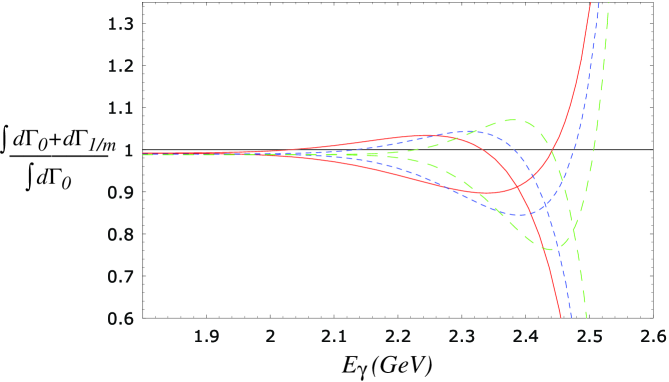
Figure 2: Partially integrated rate normalized to the leading twist result. The three lines with a peak correspond to $\rho_{2}=(500\mbox{ MeV})^{3}$, and $\bar{\Lambda}=570$ MeV (solid line), $\bar{\Lambda}=470$ MeV (short-dashed line) $\bar{\Lambda}=370$ MeV (long-dashed line). The two lines with a dip have $\rho_{2}=-(500\mbox{ MeV})^{3}$ and $\bar{\Lambda}=470$ MeV (dashed line), $\bar{\Lambda}=370$ MeV (dotted line).

4 PART III: “New Physics” in $b\to s\gamma$

In the Standard Model, $b\to s\gamma$ is a loop-induced process; it thus has considerable sensitivity to new physics effects. However, as already pointed out in the introduction, any $B$ physics experiment tests the coefficients $c_{i}$ appearing in the effective Hamiltonian (1) and thus all the information on new effects is encoded in combinations of the low-energy parameters $c_{i}$, which have to be computed in the Standard Model with the best possible accuracy. Comparing this to $B$ decay data, it will clearly be impossible to find clean evidence for some specific scenario of new physics.

At present, no significant deviation from the Standard Model has been observed in $B\to X_{s}\gamma$ nor in any other $B$ decay. Given that there are processes that are sensitive to new effects, $B$ physics (and $b\to s\gamma$ in particular) can contribute to constrain new physics scenarios.

Keeping this in mind one may try various scenarios of new physics and calculate the effects on $b\to s\gamma$, i.e. calculate the coefficients of the low energy effective Hamiltonian (1) in specific scenarios. There is an enormous variety of models for physics beyond the Standard Model on the market, and is is impossible to cover all these ideas.

For that reason I shall only consider two examples, which are instructive and demonstrate the kind of sensitivity one may expect. In the next subsection I shall consider the Type-II two-Higgs doublet model and in subsection 4.2 I shall discuss a few recent papers on supersymmetry with large values of $\tan\beta$.

4.1 Two-Higgs-Doublet Model (Type II)

One popular and consistent way to extend the Standard Model is to add one or more Higgs doublets. This can be done in various ways, but one well motivated way is to have two Higgs doublets where one doublet gives the mass to the up quarks, the other doublet to the down quarks.

Figure 3: The branching ratio for $B\to X_{s}\gamma$ as a function of the charged Higgs mass; figure taken from [29].

Figure 4: The $\tan\beta$-$M_{H^{+}}$ plane; contours indicate different experimental values for $B\to X_{s}\gamma$; figure taken from [29].

Out of the eight degrees of freedom of the Higgs sector, three are needed to give mass to the heavy weak bosons, while the other five become physical states. In particular, the spectrum contains a charged Higgs boson, which appears in the loops relevant to $b\to s\gamma$. The first analysis of this decay in this type of two-Higgs doublett model has been performed in [28].

The parameters of this model are the ratio of the two vacuum expectation values (usually expressed as $\tan\beta=v_{1}/v_{2}$), the mass $M_{H^{+}}$ of the charged Higgs boson, all other parameters are irrelevant for our discussion.

In fig. 3 (taken from [29]) the branching ratio of $b\to s\gamma$ is plotted as a function of the charged Higgs mass, for three different values of the renormalization scale $\mu$.

In fig. 4 (taken from [29]) we plot contours in the $\tan\beta$–$M_{H^{+}}$ plane for different values of the $B\to X_{s}\gamma$ branching ratio. From this figure it becomes clear that there is no large effect induced by enlarging $\tan\beta$. One may derive bounds on the charged Higgs mass independently of $\tan\beta$; the current bound is $M_{H^{+}}>314$ GeV at 95% CL [30]. This does not yet include the new CLEO result [2], which will move the bound to even higher values.

4.2 Supersymmetry with large $\tan\beta$

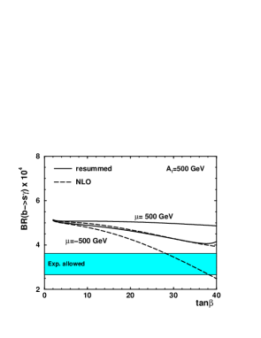
Figure 5: The rate for $B\to X_{s}\gamma$ versus $\tan\beta$; for the values of the parameters see text. Figure taken from [33].

If supersymmetry were an exact symmetry, $b\to s\gamma$ would vanish, owing to the cancellations between particles and sparticles [31]. This means that $b\to s\gamma$ tests the breaking of supersymmetry. Clearly many different scenarios for this symmetry breaking can be invented, having complicated flavour structure.

Again I shall pick an example from a recent analysis [32, 33]. In these papers it has been pointed out that $B\to X_{s}\gamma$ can indeed be enhanced in scenarios whith large $\tan\beta$. Working in the MSSM with a flavour-diagonal supersymmetry-breaking sector, the relevant parameters are the charged Higgs mass $M_{H^{+}}$, the light stop mass $m_{\tilde{t}_{1}}$, the supersymmetric $\mu$ parameter, and the parameter $A_{t}$ from the sector of soft-supersymmetry breaking.

For large $\tan\beta$, renormalization group methods may be used to resum these terms [33] and one may confront these results with the recent data. In fig. 5 (taken from [33]) we plot the rate for $B\to X_{s}\gamma$ as a function of $\tan\beta$ for $\mu=\pm 500$ GeV; the values of the other parameters are $M_{H^{+}}=200$ GeV, $m_{\tilde{t}_{1}}=250$ GeV, all other sparticle masses being at 800 GeV.

A similar plot can be made for negative $A_{t}$, but for the parameters chosen here this scenario is already practically excluded.

Given such a scenario, one may also scan over some range for the parameters and identify regions that are still allowed by the experimental constraints. In fig. 6 such a scan was performed with $m_{\tilde{t}_{2}}\leq m_{\tilde{t}_{1}}\leq 1$ TeV, $m_{\tilde{\chi}_{2}^{+}}\leq m_{\tilde{\chi}_{1}^{+}}\leq 1$ TeV, $|A_{t}|\leq 500$ GeV, all other sparticle masses being 1 TeV.

Clearly $B\to X_{s}\gamma$ places significant constraints on the parameter space of certain supersymmetric scenarios; however, these studies have been performed with a flavour diagonal supersymmetry-breaking sector. An analysis witout this constraint can be found in [34]

Figure 6: Allowed range in the $M_{H^{+}}$–$M_{\tilde{\chi}_{2}}$ plane for different values of $\tan\beta$ for two values of $m_{\tilde{t}_{2}}$. Figure taken from [33].

5 Conclusion

The inclusive radiative rare decay $B\to X_{s}\gamma$ is under reasonable theoretical control; the latest theoretical prediction [18] is slightly higher than (7)

$$Br_{th}(B\to X_{s}\gamma)=(3.71\pm 0.30)\times 10^{-4}\,,$$

where the difference originates from a different value for the ratio $m_{c}/m_{b}$; while [16] use the ratio of pole masses, in [18] $m_{c}^{\overline{MS}}/m_{b}^{Pole}$ is is used as an “educated guess” of NNLO corrections.

The latest (combined) experimental result is [18]

$$Br_{exp}=(B\to X_{s}\gamma)=(2.96\pm 0.35)\times 10^{-4}\,,$$ (24)

which is in agreement with theory within $1.6\sigma$.

The theoretical uncertainty is mainly determined by our ignorance of some of the input parameters (quark masses, mixing angles) and to some extent also by the uncertainty of higher-order radiative corrections. Improving the current theoretical uncertainty will be very difficult with current theoretical tools.

References

- [1] M. S. Alam et al. [CLEO Collaboration], Phys. Rev. Lett. 74, 2885 (1995).
- [2] E. Thorndike, these proceesdings
- [3] A. Lyon, these proceedings
- [4] T. E. Coan et al. [CLEO Collaboration], hep-ex/0010075.
- [5] A. Ali, G. F. Giudice and T. Mannel, Z. Phys. C 67, 417 (1995) [hep-ph/9408213].
- [6] A. V. Manohar and M. B. Wise, Cambridge Monographs on Particle Physics, Nuclear Physics, and Cosmology, Vol. 10.
- [7] N. Isgur and M. B. Wise, CEBAF-TH-92-10, appeared in: Stone, S. (ed.): B physics, World Scientific 1994, p. 158-209.
- [8] M. Neubert, Phys. Rept. 245, 259 (1994) [hep-ph/9306320].
- [9] I. Bigi, M. Shifman and N. Uraltsev, Ann. Rev. Nucl. Part. Sci. 47, 591 (1997) [hep-ph/9703290].
- [10] T. Mannel, Rept. Prog. Phys. 60, 1113 (1997).
- [11] K. Chetyrkin, M. Misiak and M. Munz, Phys. Lett. B 400, 206 (1997) [hep-ph/9612313].
- [12] A. Ali and C. Greub, Z. Phys. C 49, 431 (1991).
- [13] K. Adel and Y. Yao, Phys. Rev. D 49, 4945 (1994) [hep-ph/9308349].
- [14] C. Greub, T. Hurth and D. Wyler, hys. Lett. B 380, 385 (1996) [hep-ph/9602281], Phys. Rev. D 54, 3350 (1996) [hep-ph/9603404].
- [15] A. Czarnecki and W. J. Marciano, Phys. Rev. Lett. 81, 277 (1998) [hep-ph/9804252].
- [16] A. L. Kagan and M. Neubert, Eur. Phys. J. C 7, 5 (1999) [hep-ph/9805303].
- [17] A. J. Buras, M. Misiak, M. Munz and S. Pokorski, Nucl. Phys. B 424, 374 (1994) [hep-ph/9311345].
- [18] M. Misiak, talk given at the “XXVIII Rencontres de Moriond”, 10 - 17 March 2001, Les Arcs, France.
- [19] M. B. Voloshin, Phys. Lett. B 397, 275 (1997) [hep-ph/9612483], A. K. Grant, A. G. Morgan, S. Nussinov and R. D. Peccei, Phys. Rev. D 56, 3151 (1997) [hep-ph/9702380].
- [20] G. Buchalla, G. Isidori and S. J. Rey, Nucl. Phys. B 511, 594 (1998) [hep-ph/9705253].
- [21] Z. Ligeti, L. Randall and M. B. Wise, Phys. Lett. B 402, 178 (1997) [hep-ph/9702322].
- [22] M. Neubert, Phys. Rev. D 49, 4623 (1994) [hep-ph/9312311].
- [23] I. I. Bigi, M. A. Shifman, N. G. Uraltsev and A. I. Vainshtein, Int. J. Mod. Phys. A 9, 2467 (1994) [hep-ph/9312359].
- [24] A. K. Leibovich, I. Low and I. Z. Rothstein, Phys. Lett. B 486, 86 (2000) [hep-ph/0005124].
- [25] T. Mannel and S. Recksiegel, Phys. Rev. D 60, 114040 (1999) [hep-ph/9904475].
- [26] F. De Fazio and M. Neubert, JHEP9906, 017 (1999) [hep-ph/9905351].
- [27] C. W. Bauer, M. Luke and T. Mannel, hep-ph/0102089.
- [28] M. Ciuchini, G. Degrassi, P. Gambino and G. F. Giudice, two-Higgs doublet model,” Nucl. Phys. B 527 (1998) 21 [hep-ph/9710335].
- [29] F. M. Borzumati and C. Greub, Phys. Rev. D 58, 074004 (1998) [hep-ph/9802391].
- [30] P. Gambino, as in ref. [18]
- [31] S. Ferrara and E. Remiddi, Phys. Lett. B 53, 347 (1974).
- [32] G. Degrassi, P. Gambino and G. F. Giudice, JHEP0012, 009 (2000) [hep-ph/0009337].
- [33] M. Carena, D. Garcia, U. Nierste and C. E. Wagner, Phys. Lett. B 499, 141 (2001) [hep-ph/0010003].
- [34] F. Gabbiani, E. Gabrielli, A. Masiero and L. Silvestrini, Nucl. Phys. B 477, 321 (1996) [hep-ph/9604387], F. Borzumati, C. Greub, T. Hurth and D. Wyler, Phys. Rev. D 62, 075005 (2000) [hep-ph/9911245].