1 Introduction

The Tau–Charm Factory, a high–luminosity ($\sim 10^{33}\;\mbox{cm}^{-2}\;\mbox{s}^{-1}$) $e^{+}e^{-}$ collider with a centre–of–mass energy near the $\tau^{+}\tau^{-}$ production threshold, has been proposed [1, 2] as a powerful tool to perform high–precision studies of the $\tau$ lepton, charm hadrons and the charmonium system [3, 4]. In recent years, this energy region has been only partially explored by the Chinese BEBC machine ($\sim 10^{31}\;\mbox{cm}^{-2}\;\mbox{s}^{-1}$). The possibility to operate the Cornell CESR collider around the $\tau^{+}\tau^{-}$ threshold [5] has revived again the interest on Tau–Charm Factory physics [6].

A precise understanding of the $e^{+}e^{-}\to\tau^{+}\tau^{-}$ production cross section near threshold is clearly required. The accurate experimental analysis of this observable could allow to improve the present measurement [7] of the $\tau$ lepton mass. The cross section $\sigma(e^{+}e^{-}\to\tau^{+}\tau^{-})$ has already been analysed to ${\cal O}(\alpha^{3})$ in refs. [8, 9, 10], including a resummation of the leading Coulomb corrections.

The recent development of non-relativistic effective field theories of QED (NRQED) and QCD (NRQCD) [11] has allowed an extensive investigation of the threshold production of heavy flavours at $e^{+}e^{-}$ colliders. The threshold $b\bar{b}$ [12, 13, 14] and $t\bar{t}$ [15] production cross sections have been computed to the next-to-next-to-leading order (NNLO) in a combined expansion in powers of $\alpha_{s}$ and the fermion velocities. Making appropriate changes, those calculations can be easily applied to the study of $\tau^{+}\tau^{-}$ production.

In this paper we will compile and analyse the known higher–order corrections to the $\tau^{+}\tau^{-}$ production cross section. Although some ${\cal O}(\alpha^{4})$ contributions have not been computed yet, the dominant NNLO corrections can be already incorporated to the numerical predictions. One can then achieve a theoretical precision better than 0.1%.

The perturbative ${\cal O}(\alpha^{3})$ and ${\cal O}(\alpha^{4})$ contributions are discussed in section 2. Section 3 contains the relevant non-relativistic corrections at low velocities, generating ${\cal O}(\alpha^{n}/v^{m})$ effects. The photon vacuum–polarization and the initial state radiation contributions are accounted for in sections 4 and 5, respectively. In section 6, electroweak corrections are shown to be negligible. The numerical results for the $e^{+}e^{-}\to\tau^{+}\tau^{-}$ cross section and our final conclussions are given in section 7. Some technical details and detailed formulae are relegated to the appendices.

2 The Perturbative Calculation up to ${\cal O}(\alpha^{4})$

A NNLO analysis of a QED quantity, following perturbation theory in the number of loops, implies that contributions up to ${\cal O}(\alpha^{4})$ should be taken into account. Let us review the terms contributing to the total cross section of $\tau$ production in $e^{+}e^{-}$ annihilation up to this order.

At lowest order in QED, the $\tau$ leptons are produced by one-photon exchange in the s-channel, and the total cross section formula reads

$$\sigma_{\mbox{\tiny$B$}}(e^{+}\,e^{-}\to\tau^{+}\,\tau^{-})={{2\pi\,\alpha^{2}}\over{3s}}\,v\,(3-v^{2})~{}~{},$$ (1)

where $v=\sqrt{1-4M^{2}/s}$ is the velocity of the final $\tau$ leptons in the center-of-mass frame of the $e^{+}\,e^{-}$ pair and $M\equiv m_{\tau}$ is the $\tau$ mass. $v$ is an adequate expansion parameter for observables evaluated at energies close to the production threshold, since its value goes to zero as we approach this point. This makes $\sigma_{\mbox{\tiny$B$}}$ vanish in that limit, being the global factor $v$ in (1) of kinematic origin. The quantum numbers of the $\tau^{+}\,\tau^{-}$ pair are those of the photon, $J^{PC}=1^{--}$, which corresponds to allowed $\tau^{+}\,\tau^{-}$ states ${}^{3}S_{1}$ and ${}^{3}D_{1}$ in spectroscopic notation ${}^{2S+1}L_{J}$.

Electromagnetic corrections of ${\cal O}(\alpha)$ to $\sigma_{\mbox{\tiny$B$}}$ arise from the interference between the tree level result and the following 1-loop amplitudes:

• ${\cal O}(\alpha)$ corrections to the $e^{+}e^{-}\gamma$ vertex,

• ${\cal O}(\alpha)$ corrections to the $\tau^{+}\tau^{-}\gamma$ vertex,

• vacuum polarization,

• box diagrams (2-photon production).

The contributions from i) and ii) are usually expressed in terms of the Dirac and Pauli form factors at one loop [16]. The corrections to the photon propagator iii) are divided into two pieces: the leptonic contribution ($\ell=e,\mu,\tau$), which can be calculated perturbatively in QED, and the hadronic contribution, where QCD corrections make a perturbative estimate at low energies unreliable. The hadronic vacuum polarization can be related to the total cross section of hadron production by means of a dispersion relation. Finally, the interference of the tree–level amplitude with box diagrams iv) does not contribute to the total cross section, by virtue of Furry’s Theorem.

Besides the above virtual radiative corrections, the cross section of ${\cal O}(\alpha^{3})$ corresponding to the process of real photon emission, $e^{+}\,e^{-}\to\tau^{+}\,\tau^{-}\,\gamma$ , must be added. The Bremsstrahlung photon can be emitted by the initial or final fermion lines, but there is no contribution to the total cross section from the interference between both sets of diagrams, again due to Furry’s Theorem. We clearly see that there is no overlap between initial and final state radiative corrections for the total cross section up to ${\cal O}(\alpha^{3})$. A compilation of analytical expressions for all the terms mentioned above is found in Ref. [9].

Let us consider next ${\cal O}(\alpha^{2})$ electromagnetic corrections to the Born cross section. They come from several sources:

• Interferences between the one-loop diagrams mentioned previously. The total cross section contributions from interferences between i), ii) and iii) with box diagrams are again zero. The first term involving two-photon $\tau$ production comes from the square amplitude of the box diagrams.

• Interferences between the Born term and the following two-loop amplitudes: the electron and the $\tau$ vertex two-loop corrections, contained in the expressions of the electromagnetic form factors, ${\cal O}(\alpha)$ corrections to the vacuum polarization, and three-photon production diagrams, for which only the real part is needed.

• The ${\cal O}(\alpha^{4})$ Bremsstrahlung cross section, coming from the interference between tree-level and one-loop diagrams with one radiated photon, and from tree-level diagrams with two photons attached in any of the fermion lines, corresponding to the process $e^{+}\,e^{-}\to\tau^{+}\,\tau^{-}\,\gamma\gamma$. It is no longer true, at this order, that initial and final state real radiation could not interfere.

Recall that the spectral density $\mbox{Im}\Pi_{\mbox{\tiny em}}(s)$ built from the electromagnetic current of the $\tau$ leptons collects all final–state interactions, including both virtual and real radiation, for single-photon production, that is

$$\tilde{\sigma}(e^{+}e^{-}\to\gamma^{*}\to\tau^{+}\,\tau^{-})\,=\,\frac{48\pi^{2}\alpha^{2}}{3s}\,\mbox{Im}\Pi_{\mbox{\tiny em}}(s)\,,$$ (2)

where the tilde on $\sigma$ distinguishes it from the physical total cross section which includes all kind of corrections. Relation (2) results from a direct application of the optical theorem, and is more commonly written as the ratio

$$R_{\mbox{\tiny$em$}}(s) = \frac{\tilde{\sigma}(e^{+}e^{-}\to\gamma^{*}\to\ell^{+}\ell^{-})}{\sigma_{pt}}\,=\,12\pi\,\mbox{Im}\Pi_{\mbox{\tiny em}}(s)\,,$$ (3)

i.e., normalizing $\tilde{\sigma}$ to the point cross section $\sigma_{pt}\,=\,\frac{4\pi\alpha^{2}}{3s}$. The ratio $R_{\mbox{\tiny$em$}}$ is well suited for studying the non-relativistic dynamics of the $\tau^{+}\,\tau^{-}$ pair, as it fully contains the final–state interaction. Therefore, the threshold behaviour of the total cross section will be ruled by the expansion of $R_{\mbox{\tiny$em$}}$ at low velocities. The perturbative QED expression of $R_{\mbox{\tiny$em$}}$ is given in Appendix A up to NNLO in the combined expansion in powers of $\alpha$ and $v$.

As long as we do not care about multiple photon production of $\tau$ leptons, neither consider interference between initial and final state radiation, it is possible to factorize the total cross section as an integration over the product of separate pieces including initial, intermediate and final state corrections:

$$\sigma(s)=\int^{s}\,F(s,w)\,\bigg{|}\frac{1}{1+e^{2}\Pi{\mbox{\tiny em}}(w)}\bigg{|}^{2}\,\tilde{\sigma}(w)\,dw\,.$$ (4)

The radiation function $F(s,w)$ [17] describes initial state radiation, including virtual corrections, and $\sqrt{s}$ is the total energy in the center-of-mass frame. The integration emerges to account for the effective energy loss due to photon emission from the $e^{+}\,e^{-}$ pair. As previously mentioned, (4) is an exact relation for the total cross section only up to ${\cal O}(\alpha^{3})$, but it includes the largest corrections coming from the emission of an arbitrary number of initial photons, which can sizeably suppress the total cross section. The ${\cal O}(\alpha^{4})$ contributions not included in this analysis are those coming from two- and three-photon production diagrams, for which no velocity enhancement is expected in the threshold region and so represent pure ${\cal O}(\alpha^{2})$ corrections $\sim 0.005\%$, and the interferences between 2-photon Bremsstrahlung diagrams overlapping initial and final state radiation. However, we shall argue in section 3 that Bremsstrahlung contributions start at NNNLO in the combined expansion in $\alpha$ and $v$, and so they are beyond the scope of our analysis.

3 Non-Relativistic Corrections: NRQED

We now focus on the behaviour of the total cross section in the region just above the production threshold, where the small velocity of the produced $\tau$ leptons is another relevant parameter, besides $\alpha$. The final–state $\tau^{+}\tau^{-}$ interactions are encoded in the electromagnetic form factors. Written in terms of $v$, their expressions at one and two loops [18] show the existence of ${\cal O}\left(\frac{\alpha}{v}\right)$ and ${\cal O}\big{(}\frac{\alpha^{2}}{v^{2}}\big{)}$ power-like divergences in the limit $v\to 0$. This is a general result for any number of loops: diagrams with $n$ uncrossed photons exchanged between the produced leptons generate singular terms proportional to $\left(\frac{\alpha}{v}\right)^{n}$, known as Coulomb singularities, which lead to a breakdown of the QED perturbative series in $\alpha$ when $v\to 0$. Resummation of such terms is therefore mandatory, and it was done a long time ago [19], resulting in the well-known Sommerfeld factor

$$|\Psi_{c,\mbox{\tiny E}}(0)|^{2}\,=\,\frac{\alpha\pi/v}{1-\mbox{exp}(-\alpha\pi/v)}\,,$$ (5)

multiplying the Born cross section (1). This factor corresponds to the wave function at the origin, solution of the Schrödinger equation, of two conjugate charged particles of mass $M$ interacting through a Coulomb potential for positive energies $E=Mv^{2}$. The appearence of this factor in the cross section can be intuitively understood, since the Coulomb interaction modifies the scattered wave function of the lepton pair. The $1/v$ behaviour of this factor makes the cross section at threshold finite.

We clearly see that a NNLO calculation of the cross section in the kinematic region where $\alpha\sim v$ has to account for all terms proportional to $v\,(\alpha/v)^{n}\times[1;\alpha;v;\alpha^{2};\alpha v;v^{2}]$ with $n=1,2,\dots$ The leading divergences (i.e. $\left(\frac{\alpha}{v}\right)^{n}$, $n>1$) can be treated by using well-known results from non-relativistic quantum mechanics, but a systematic way to calculate higher-order corrections in this regime, such as $\left(\frac{\alpha}{v}\right)^{n}\times[v,v^{2},\cdots]$, seems to be far from obvious, at least from the point of view of covariant perturbation theory in the number of loops. An adequate description would come from a simplified theory which keeps the relevant physics at the scale $Mv\sim M\alpha$, characteristic of the Coulomb interaction, allowing for a clear and systematic identification of leading contributions.

NRQED [11] was designed precisely for this purpose. It is an effective field theory of QED at low energies, applicable to fermions in non-relativistic regimes, i.e. with typical momenta $p/M\sim v\ll 1$. Interactions contained in the NRQED Lagrangian (B.1) have a definite velocity counting but propagators and loop integrations can also generate powers of $v$. With appropriate counting rules at hand, one can prove that all interactions between the non-relativistic pair $\tau^{+}\tau^{-}$ can be described up to NNLO in terms of time-independent potentials [20], derived from the low-energy Lagrangian. It can also be shown that the contributions to the total cross section from diagrams with real photons emitted from the produced heavy leptons begin at NNNLO .

The key observable to study threshold effects in $\tau^{+}\tau^{-}$ production is the 2-point function, $\Pi_{\mbox{\tiny em}}(s)$ calculated at NNLO. Its fully covariant expression is written as the time ordered correlator of two electromagnetic QED currents of the $\tau$ lepton $j^{\mu}={\bar{\tau}}\gamma^{\mu}\tau$:

$$R_{\mbox{\tiny$em$}}(q^{2})=\frac{4\pi}{q^{2}}\,\,\mbox{Im}\Bigl{[}-i\int d^{4}x\,e^{iqx}\,\langle 0|T\left(j^{\mu}(x)\,j_{\mu}(0)^{\dagger}\right)|0\rangle\Bigr{]}\,.$$ (6)

Inserting the effective low-energy expression for the QED current, eq. (B.2), in the last equation, one can arrive to the basic relation between the spectral density at NNLO and the non-relativistic Green’s functions [22]:

$$R^{\mbox{\tiny NNLO}}_{\mbox{\tiny$em$}}(q^{2})=\frac{6\,\pi}{M^{2}}\,\,\mbox{Im}\Big{(}C_{1}\,G({\mbox{\boldmath$0$}},{\mbox{\boldmath$0$}};E)\,-\frac{4E}{3M}\,G_{c}({\mbox{\boldmath$0$}},{\mbox{\boldmath$0$}};E)\Big{)}\,,$$ (7)

with $C_{1}$ a short distance coefficient to be determined by matching full and effective theory results. The details of this derivation are found in Appendix B.

The Green’s function $G$ obeys the Schrödinger equation corresponding to a two-body system interacting through potentials derived from ${\cal{L}}_{\mbox{\tiny NRQED}}$ at NNLO, that means suppressed at most by $\alpha^{2},\alpha/M$ or $1/M^{2}$, as dictated by the counting rules. Such potentials have been calculated in the literature [23, 24, 25], and in configuration space they read

$$V_{c}(r) = -\,\frac{\alpha(\mu_{s})}{r}\,\bigg{\{}\,1+\bigg{(}\frac{\alpha(\mu_{s})}{4\,\pi}\bigg{)}\,\Big{[}\,2\,\beta_{1}\,\ln(\tilde{\mu}\,r)+a_{1}\,\Big{]}$$

$$+\,\bigg{(}\frac{\alpha(\mu_{s})}{4\,\pi}\bigg{)}^{2}\,\Big{[}\,\beta_{1}^{2}\,\Big{(}\,4\,\ln^{2}(\tilde{\mu}\,r)+\frac{\pi^{2}}{3}\,\Big{)}+2\,\Big{(}2\,\beta_{1}\,a_{1}+\beta_{2}\Big{)}\,\ln(\tilde{\mu}\,r)+a_{2}\,\Big{]}\,\bigg{\}}\,,$$

$$V_{\mbox{\tiny BF}}({\mbox{\boldmath$r$}}) = \frac{\alpha(\mu_{s})\,\pi}{M^{2}}\,\,\delta^{(3)}({\mbox{\boldmath$r$}})+\frac{\alpha(\mu_{s})}{2\,M^{2}r}\,\Big{[}\,{\mbox{\boldmath$\nabla$}}^{2}+\frac{1}{r^{2}}{\mbox{\boldmath$r$}}\,({\mbox{\boldmath$r$}}\,{\mbox{\boldmath$\nabla$}}){\mbox{\boldmath$\nabla$}}\,\Big{]}$$ (9)

$$-\,\frac{\alpha(\mu_{s})}{2\,M^{2}}\,\left[\,\frac{{\mbox{\boldmath$S$}}^{2}}{r^{3}}-\,3\,\frac{\big{(}{\mbox{\boldmath$S$}}\,{\mbox{\boldmath$r$}}\,\big{)}^{2}}{r^{5}}\,-\frac{4\pi}{3}\big{(}2\,{\mbox{\boldmath$S$}}^{2}-3\big{)}\,\delta^{(3)}({\mbox{\boldmath$r$}})\,\right]+\,\frac{3\,\alpha(\mu_{s})}{2\,M^{2}\,r^{3}}\,{\mbox{\boldmath$L$}}\,{\mbox{\boldmath$S$}}\,,$$

$$V_{\mbox{\tiny An}}({\mbox{\boldmath$r$}}) = \frac{\alpha(\mu_{s})\,\pi}{M^{2}}\,{\mbox{\boldmath$S$}}^{2}\,\delta^{(3)}({\mbox{\boldmath$r$}})\,.$$ (10)

$$V_{\mbox{\tiny Ki}}({\mbox{\boldmath$r$}}) = -\frac{{\mbox{\boldmath$\nabla$}}^{4}}{4M^{3}}\,.$$ (11)

Here $\alpha(\mu_{s})$ denotes the electromagnetic coupling constant renormalized in the $\overline{MS}$ scheme at the scale $\mu_{s}\equiv\mu_{\mbox{\tiny$soft$}}$. The latter is the renormalization scale set for the ${\cal O}(\alpha)$ and ${\cal O}(\alpha^{2})$ corrections to the Coulomb potential (LABEL:coulombpotential), as determined in [23] and [24], respectively. Note that these corrections involve ultraviolet divergent light fermion loops ($m_{f}\ll M$), which cannot be accurately described within NRQED. The scale $\tilde{\mu}$ is equal to $\mu_{\mbox{\tiny$soft$}}\,e^{\gamma_{\mbox{\tiny E}}}$, with $\gamma_{\mbox{\tiny E}}$ the Euler constant, and the rest of coefficients in (LABEL:coulombpotential) take the values

$$\beta_{1} = -\frac{4}{3}\,n_{\ell}\,,\hskip 28.45274pt\beta_{2}=-4\,n_{\ell}\,,$$ (12)

$$a_{1} = -\frac{20}{9}\,n_{\ell}\,,\hskip 28.45274pta_{2}=-\bigg{(}\,\frac{55}{3}-16\,\zeta_{3}\,\bigg{)}\,n_{\ell}+\bigg{(}\,\frac{20}{9}\,n_{\ell}\,\bigg{)}^{2}\,.$$ (13)

The constants $\beta_{1}$ and $\beta_{2}$ are the one- and two-loop coefficients of the QED beta function in the $\overline{MS}$ scheme defined as

$$\frac{d\ln\alpha}{d\ln\mu^{2}}=\beta(\alpha)=\beta_{1}\frac{\alpha}{4\pi}+\beta_{2}\bigg{(}\frac{\alpha}{4\pi}\bigg{)}^{2}+\cdots$$ (14)

The number of active lepton flavors $n_{\ell}$ would be equal to two for interacting $\tau$’s. If quark loops are included we should substitute $n_{\ell}\to n_{f}\equiv(n_{\ell}+N_{c}\sum_{q}Q_{q}^{2})$, being $Q_{q}$ the electromagnetic charge of the quark $q$ (with mass lower than $M$).

The Breit-Fermi potential $V_{\mbox{\tiny BF}}$ (see e.g. [25]) has been written in terms of the total spin $S$ and angular momentum $L$ of the lepton pair. At NNLO, the heavy leptons are only produced in triplet S-wave states, so we just need to consider the corresponding projection of the $V_{\mbox{\tiny BF}}$ potential, (i.e. make ${\mbox{\boldmath$S$}^{2}}=2$ and ${\mbox{\boldmath$L$}}=0$ in (9)). $V_{\mbox{\tiny An}}$ is a NNLO piece derived from the first contact term written in ${\cal{L}}_{\mbox{\tiny NRQED}}$, eq. (B.1), which reproduces the QED tree level s-channel diagram for the process $\ell^{+}\ell^{-}\to\ell^{+}\ell^{-}$. In QCD this diagram connects $q\bar{q}$ color-octet states, so this piece is not present in recent papers devoted to threshold electromagnetic quark production, where $q\bar{q}$ pairs can only be produced in color-singlet states. Finally, the term (11) is the first relativistic correction to the kinetic energy.

The Green’s function at NNLO will therefore satisfy the Schrödinger equation 

$$\bigg{(}-\frac{{\mbox{\boldmath$\nabla$}}^{2}}{M}-\frac{{\mbox{\boldmath$\nabla$}}^{4}}{4M^{3}}+V_{c}({\mbox{\boldmath$r$}})+V_{\mbox{\tiny BF}}({\mbox{\boldmath$r$}})+V_{\mbox{\tiny An}}({\mbox{\boldmath$r$}})-E\,\bigg{)}\,G({\mbox{\boldmath$r$}},{\mbox{\boldmath$r$}^{\prime}},E)\,=\,\delta^{(3)}({\mbox{\boldmath$r$}}-{\mbox{\boldmath$r$}^{\prime}})\,.$$ (15)

A solution of eq. (15) must rely on numerical or perturbative techniques. In the QED case, a significant difference between both approaches is not expected, being $\alpha$ such a small parameter . Consequently we will follow the perturbative approach, using recent results by Hoang, Penin and others [13, 22, 26], who calculated the NLO and NNLO corrections to the Green’s function analytically, via Rayleigh-Schrödinger time-independent perturbation theory around the known LO Coulomb Green’s function:

$$G({\mbox{\boldmath$x$}},{\mbox{\boldmath$y$}};E)\,=\,{G}_{c}({\mbox{\boldmath$x$}},{\mbox{\boldmath$y$}};E)\,+\,\delta G({\mbox{\boldmath$x$}},{\mbox{\boldmath$y$}};E)\,,$$

$$\delta G({\mbox{\boldmath$x$}},{\mbox{\boldmath$y$}};E)\,=\,-\int d^{3}\mbox{\boldmath$z$}\,{G}_{c}({\mbox{\boldmath$x$}},{\mbox{\boldmath$z$}};E)\,(H-H_{0})\,{G}_{c}({\mbox{\boldmath$z$}},{\mbox{\boldmath$y$}};E)\,+\cdots\,$$

$$=-\int d^{3}\mbox{\boldmath$z$}\,{G}_{c}({\mbox{\boldmath$x$}},{\mbox{\boldmath$z$}};E)\,\bigg{(}-\frac{{\mbox{\boldmath$\nabla$}}^{4}}{4M^{3}}+V_{\mbox{\tiny BF}}({\mbox{\boldmath$z$}})+V_{\mbox{\tiny An}}({\mbox{\boldmath$z$}})+V_{c}^{\tiny(1)}({\mbox{\boldmath$z$}})+V_{c}^{\tiny(2)}({\mbox{\boldmath$z$}})\bigg{)}\,{G}_{c}({\mbox{\boldmath$z$}},{\mbox{\boldmath$y$}};E)\,+\cdots$$

$$\hskip 62.59596pt\,=\,\delta_{\mbox{\tiny Ki,BF}}G+\delta_{\mbox{\tiny An}}G+\delta^{\mbox{\tiny NLO}}_{\tiny 1}G+\delta_{\tiny 2}G+\delta^{\mbox{\tiny NNLO}}_{\tiny 1}G+\,\cdots\,.$$ (16)

Here $H_{0}=-{\mbox{\boldmath$\nabla$}}^{2}/M+V_{c}^{\mbox{\tiny LO}}(r)$ is the pure Coulomb Hamiltonian. We refer the reader to Appendix C for complete expressions of $G_{c}$ and the different $\delta G$’s, as calculated in the literature, and for a full discussion about the regularization procedure. Let us just quote here that the Sommerfeld factor (5), which appears in the LO cross section can be easily recovered from the basic relation (7), if one reminds the spectral representation of the Green’s function

$$G({\mbox{\boldmath$r$}},{\mbox{\boldmath$r$}^{\prime}};E)=\sum_{n}\,\frac{\Psi_{n}({\mbox{\boldmath$r$}})\,\Psi_{n}^{*}({\mbox{\boldmath$r$}^{\prime}})}{E_{n}-E-i\epsilon}\,+\,\int\frac{d^{3}{\mbox{\boldmath$k$}}}{(2\pi)^{3}}\,\frac{\Psi_{k}({\mbox{\boldmath$r$}})\,\Psi_{k}^{*}({\mbox{\boldmath$r$}^{\prime}})}{E_{k}-E-i\epsilon}\,,$$ (17)

with $\Psi_{n}({\mbox{\boldmath$r$}})$ the bound state’s wave functions ($E_{n}<0$), and $\Psi_{k}({\mbox{\boldmath$r$}})$ corresponding to eigenfunctions of $H$ with $E_{k}={\mbox{\boldmath$k$}}^{2}/M>0$. The LO spectral density is proportional to the imaginary part of the Coulomb Green’s function, and so, from (17), proportional to $|\Psi_{c,\mbox{\tiny E}}(0)|^{2}$, i.e. to the solution at the origin of the Schrödinger equation with the LO Coulomb potential.

Finally, the short distance coefficient $C_{1}$ must be fixed. The “direct matching procedure” [27] allows a straightforward determination of $C_{1}$, by comparing the NNLO non-relativistic expression (7) with the result (A.1) for $R_{\mbox{\tiny$em$}}$, calculated in full QED keeping terms up to ${\cal O}(\alpha^{2})$ and NNLO in the velocity expansion. The short distance coefficient $C_{1}$ is then expressed as a perturbative series in $\alpha(\mu_{\mbox{\tiny$hard$}})$

$$C_{1}(M,\mu_{\mbox{\tiny$hard$}},\mu_{\mbox{\tiny$fac$}})\,=\,1+\left(\frac{\alpha(\mu_{\mbox{\tiny$hard$}})}{\pi}\right)\,c_{1}^{(1)}+\left(\frac{\alpha(\mu_{\mbox{\tiny$hard$}})}{\pi}\right)^{2}\,c_{1}^{(2)}(\mu_{\mbox{\tiny$hard$}},\mu_{\mbox{\tiny$fac$}})+\dots\,,$$ (18)

where we have anticipated that $c_{1}^{(1)}$ does not depend on any scale. The renormalization point $\mu_{\mbox{\tiny$hard$}}$, chosen for $\alpha_{\mbox{\tiny$\overline{MS}$ }}$ in the short distance coefficient, needs not be equal to that governing the perturbative expansions of the correlators, $\mu_{\mbox{\tiny$soft$}}$, which only contains long-distance physics . The result of the matching reads [22]

$$c_{1}^{(1)} = -4$$

$$c_{1}^{(2)} = \pi^{2}\,\bigg{[}\,\kappa-\frac{4}{3\pi^{2}}n_{f}\,\ln\frac{M^{2}}{\mu_{\mbox{\tiny$hard$}}^{2}}-\frac{1}{6}\ln\frac{M^{2}}{\mu_{\mbox{\tiny$fac$}}^{2}}\,\bigg{]}\,,$$ (19)

with

$$\kappa=\bigg{[}\,\frac{1}{\pi^{2}}\,\bigg{(}\,\frac{39}{4}-\zeta_{3}\,\bigg{)}+\frac{4}{3}\ln 2-\frac{35}{18}\,\bigg{]}+\bigg{[}\,\frac{4}{9}\,\bigg{(}\,\frac{11}{\pi^{2}}-1\,\bigg{)}\,\bigg{]}+n_{f}\,\bigg{[}\,\frac{11}{9\,\pi^{2}}\,\bigg{]}\,.$$ (20)

The factorization scale $\mu_{\mbox{\tiny$fac$}}$ is introduced to separate long and short distance contributions in the process of regularization (see Appendix C for details).

4 Vacuum Polarization

We now turn over intermediate state corrections in formula (4). For a complete NNLO description of $\sigma(e^{+}e^{-}\to\tau^{+}\tau^{-})$, two-loop corrections to the photon propagator should be included. Despite having calculated the final state observable $R_{\mbox{\tiny$em$}}$ in the $\overline{MS}$ scheme, we can exploit the fact that the piece $e^{2}/\,[1+e^{2}\,\Pi_{\mbox{\tiny em}}(s)]$ is a renormalization group invariant, and so evaluate these set of corrections in the $on-shell$ scheme, where decoupling of heavy fermions is naturally implemented. The $on-shell$ renormalized vacuum polarization function is defined as

$$\Pi_{\mbox{\tiny em}}^{\mbox{\tiny$ren$}}(q^{2})\,=\,\Pi_{\mbox{\tiny em}}(q^{2})-\Pi_{\mbox{\tiny em}}(0)\,.$$ (21)

The light lepton contributions to the vacuum polarization are the standard 1- and 2-loop perturbative expressions [28]:

$$e^{2}\,\Pi_{\mbox{\tiny$e,\mu$}}(q^{2})\,=\,\bigg{(}\frac{\alpha}{\pi}\bigg{)}\Pi^{(1)}(q^{2})+\bigg{(}\frac{\alpha}{\pi}\bigg{)}^{2}\Pi^{(2)}(q^{2})+{\cal O}(\alpha^{3})\,,$$ (22)

with

$$\Pi^{(1)}(q^{2}) = \sum_{i=e,\mu}\,\frac{1}{3}\bigg{[}\frac{5}{3}-\ln\Big{(}-\frac{q^{2}}{m_{i}^{2}}\Big{)}+\frac{6m_{i}^{2}}{q^{2}}+{\cal O}\Big{(}\frac{m_{i}^{4}}{q^{4}}\Big{)}\bigg{]}\,,$$ (23)

$$\Pi^{(2)}(q^{2}) = \sum_{i=e,\mu}\,\frac{1}{4}\bigg{[}\frac{5}{6}-4\zeta_{3}-\ln\Big{(}-\frac{q^{2}}{m_{i}^{2}}\Big{)}-12\frac{m_{i}^{2}}{q^{2}}\ln\Big{(}-\frac{q^{2}}{m_{i}^{2}}\Big{)}+{\cal O}\Big{(}\frac{m_{i}^{4}}{q^{4}}\Big{)}\bigg{]}\,,$$ (24)

where we have only retained the relevant terms in the limit $m_{\ell}^{2}\ll q^{2}$ ($m_{\ell}$ are the pole light-lepton masses). For the $\tau$ contribution in the threshold vicinity $q^{2}\stackrel{{\scriptstyle>}}{{{}_{\sim}}}4M^{2}$, resummation of singular terms in the limit $v\to 0$ is mandatory. Under the assumption $\alpha\sim v$, it is clear that we need to know NLO contributions to $\Pi_{\tau}(q^{2})$, which means retaining uniquely $G_{c}$ and $\delta_{1}^{\mbox{\tiny NLO}}G$ in (16), but performing the direct matching not only for the imaginary part but also for the real part (up to ${\cal O}(\alpha)$):

$$e^{2}\Pi^{\mbox{\tiny NLO}}_{\tau}(q^{2})=\frac{2\pi\alpha}{M^{2}}\,C_{1}\bigg{(}\,{G}_{c}({\mbox{\boldmath$0$}},{\mbox{\boldmath$0$}};E)+\delta^{\mbox{\tiny NLO}}_{1}G({\mbox{\boldmath$0$}},{\mbox{\boldmath$0$}};E)\bigg{)}+\alpha\,h_{1}+\alpha^{2}h_{2}\,.$$ (25)

The one-loop coefficient $C_{1}$ was already obtained in (19), and $h_{1},h_{2}$ are fixed by demanding equality between $\mbox{Re}\,\Pi_{\tau}$ calculated in full QED and expression (25). We get

$$h_{1} = \frac{8}{9\pi}\,,$$

$$h_{2} = \frac{1}{4\,{{\pi}^{2}}}\,\left(3-\frac{21}{2}\,\zeta_{3}\right)+\frac{11}{32}-\frac{3}{4}\,\ln 2+\frac{1}{2}\,\ln\frac{M}{\mu_{\mbox{\tiny$fac$}}}\,.$$ (26)

In the hadronic sector, a perturbative estimate of the vacuum polarization in terms of free quarks is unreliable since strong interactions at low energies become non-perturbative. An alternative approach consists in relating the hadronic vacuum polarization with the total cross section $\sigma(e^{+}e^{-}\to\gamma^{*}\to had)$, by using unitarity and the analyticity of $\Pi_{\mbox{\tiny had}}(s)$:

$$\Pi_{\mbox{\tiny had}}(s) = \frac{s}{\pi}\int^{\infty}_{4m_{\pi}^{2}}dt\,\,\frac{\mbox{Im}\,\Pi_{\mbox{\tiny had}}(t)}{t(t-s-i\epsilon)}$$ (27)

$$= \frac{s^{2}}{16\pi^{3}\alpha^{2}}\,\int^{\infty}_{4m_{\pi}^{2}}dt\,\,\frac{\sigma(e^{+}e^{-}\to had)}{t(t-s-i\epsilon)}\,.$$

Usually, $\sigma(e^{+}e^{-}\to\gamma^{*}\to had)$ is conveniently parameterized and the unknown parameters fitted to experimental measurements or else related to phenomenological constants. In this paper we will make use of a parameter-free formula for $\sigma(e^{+}e^{-}\to\gamma^{*}\to had)$ in the low-energy region, where the non-perturbative effects are more important, and the perturbative result for the high energy part. Below 1 GeV, the electromagnetic production of hadrons is dominated by the $\rho$ resonance ($J^{PC}=1^{--}$) and its decay to two charged pions. The photon mediated $\pi^{+}\pi^{-}$ production cross section at a center-of-mass energy $\sqrt{s}$ is written as

$$\sigma(e^{+}e^{-}\to\pi^{+}\pi^{-})=\frac{\pi\alpha^{2}}{3s}\bigg{(}1-\frac{4m_{\pi}^{2}}{s}\bigg{)}^{3/2}\arrowvert\,F(s)\,\arrowvert^{2}\,,$$ (28)

with $F(s)$ being the pion electromagnetic form factor defined as

$$\langle\pi^{+}\pi^{-}|j^{\mu}|0{\rangle}=F(s)\,(p_{\pi^{-}}-p_{\pi^{+}})^{\mu}\,.$$

In the isospin limit, only the $I=1$ part of the quark electromagnetic current $j^{\mu}=Q_{u}\,\bar{u}\gamma^{\mu}u+Q_{d}\,\bar{d}\gamma^{\mu}d$ survives. An analytic expression for the pion isovectorial form factor was obtained in Ref. [29] using Resonance Chiral Theory [30] and restrictions imposed by analyticity and unitarity. The so-obtained $F(s)$, which provides an excellent description of experimental data up to energies of the order of 1 GeV, reads:

$$F(s) \!\!\!= \!\!\!\frac{M^{2}_{\rho}}{M^{2}_{\rho}-s-iM_{\rho}\Gamma_{\rho}(s)}\exp\Biggl{\{}\frac{-s}{96\pi^{2}f_{\pi}^{2}}\hbox{Re}\,A(m_{\pi}^{2}/s,m_{\pi}^{2}/M_{\rho}^{2})\Biggr{\}}\,,$$ (29)

where $\Gamma_{\rho}(s)$ is the off-shell width of the $\rho$ meson [31],

$$\Gamma_{\rho}(s) = {M_{\rho}\,s\over 96\pi f_{\pi}^{2}}\theta(s-4m_{\pi}^{2})\,\sigma_{\pi}^{3}$$ (30)

$$= -{M_{\rho}\,s\over 96\pi^{2}f_{\pi}^{2}}\,\hbox{Im}\left[A(m_{\pi}^{2}/s,m_{\pi}^{2}/M_{\rho}^{2})\right]\,,$$

and

$$A(m_{\pi}^{2}/s,m_{\pi}^{2}/M_{\rho}^{2})\,=\,\ln{\left(m^{2}_{\pi}/M_{\rho}^{2}\right)}+{8m^{2}_{\pi}\over s}-\frac{5}{3}+\sigma_{\pi}^{3}\,\ln{\left(\frac{\sigma_{\pi}+1}{\sigma_{\pi}-1}\right)}\,,$$

$$\sigma_{\pi}\equiv\sqrt{1-4m_{\pi}^{2}/s}\,.$$

Formula (28) will be integrated in (27) up to an upper bound $s_{\rho}\sim$ 1 GeV². For the integration region above $s_{\rho}$, we use the perturbative results of $\mbox{Im}\Pi_{\mbox{\tiny had}}$:

$$e^{2}\mbox{Im}\,\Pi_{u,d,s}(s)=\sum_{q=u,d,s}N_{c}\,Q_{q}^{2}\frac{\alpha}{3}\left[1+\frac{\alpha_{s}}{\pi}\right]\,,$$ (31)

for light quarks, in the zero mass limit, and

$$e^{2}\,\mbox{Im}\,\Pi_{c,b}(s)=\sum_{q=c,b}\theta(s-4m_{q}^{2})N_{c}\,Q_{q}^{2}\frac{\alpha}{3}\!\!\!\! \Bigg{[} \!\!\!\!\Big{(}1+\frac{2m_{q}^{2}}{s}\Big{)}\,\sqrt{1-\frac{4m_{q}^{2}}{s}}$$ (32)

$$+ \!\!\!\!\frac{\alpha_{s}}{\pi}\,C_{F}\bigg{(}\frac{3}{4}+9\frac{m_{q}^{2}}{s}+\frac{m_{q}^{4}}{s^{2}}\Big{(}\frac{5}{2}-18\ln\frac{m_{q}^{2}}{s}\Big{)}\bigg{)}\,\Bigg{]}\,,$$

for the $b$ and $c$ quarks . In both (31) and (32) the first QCD loop correction to the quark vacuum polarization has been added, with $\alpha_{s}$ the strong coupling constant. This simplified description is good enough to achieve an accuracy better than 0.1$\%$ for the $e^{+}e^{-}\to\tau^{+}\tau^{-}$ cross section.

As a test of our method to calculate the hadronic vacuum polarization, we have computed its contribution to the running of $\alpha$ at the scale $\sqrt{s}=M_{Z}$, and compared it with the results of recent analyses devoted to this subject [32, 33]. In the on-shell scheme the evolution of the electromagnetic coupling constant due to hadron polarization is commonly defined as

$$\alpha(s)=\frac{\alpha}{1-\Delta_{\mbox{\tiny had}}\alpha(s)}$$

with

$$\Delta_{\mbox{\tiny had}}\alpha(s)=-4\pi\alpha\,\mbox{Re}\left[\Pi_{\mbox{\tiny had}}(s)-\Pi_{\mbox{\tiny had}}(0)\right]\,.$$

At the scale $M_{Z}$ we get $\Delta_{\mbox{\tiny had}}\alpha(M_{Z}^{2})\times 10^{4}=268$, to be compared with the values $\Delta_{\mbox{\tiny had}}\alpha(M_{Z}^{2})\times 10^{4}=280\pm 7$ and $\Delta_{\mbox{\tiny had}}\alpha(M_{Z}^{2})\times 10^{4}=276.3\pm 1.6$, obtained in [32] and [33] respectively. Our simple estimate only deviates by 4$\%$ and 3$\%$ respectively, from those analyses. Considering that $\Pi_{\mbox{\tiny had}}$ modifies $\sigma(e^{+}e^{-}\to\tau^{+}\tau^{-})$ near threshold by roughly $1\%$, our result has a global uncertainty smaller than $0.1\%$ for the total cross section.

Let us just mention that the theoretical description of the vector form factor of the pion has been improved in a recent paper [34] using a model-independent parameterization which can fairly reproduce experimental data coming from $e^{+}e^{-}\to\pi^{+}\pi^{-}$ up to higher energies, $\sqrt{s}\stackrel{{\scriptstyle<}}{{{}_{\sim}}}1.2$ GeV. With such results, we would gain knowledge on the hadronic contribution to vacuum polarization, but its numerical effect on our final estimate would not be relevant, considering the important features of the hadronic spectrum we are leaving out by using naive QCD perturbation theory from $\sqrt{s}\sim 1.2$ GeV upwards.

5 Initial State Radiation

In this section we collect the radiative corrections to single-photon annihilation of the initial $e^{+}e^{-}$ pair. These include both virtual and real photon radiation, all of which are needed at ${\cal O}(\alpha^{2})$ in a formal NNLO analysis of $\sigma(e^{+}e^{-}\to\tau^{+}\tau^{-})$. However, for the emission of soft photons (i.e. photons whose energy do not exceed an experimental resolution $\Delta E\ll\sqrt{s}$), it is a well-known feature that the expansion parameter is not $\alpha$ but $(\alpha/\pi)\log(s/m_{e}^{2})\log(E/\Delta E)$, which may be quite large, making necessary to retain all terms of the expansion with respect to it. It is possible to perform such resummation by using an approach based on the Structure Functions formalism [17]. In this technique, the effect of initial state radiation is accounted for by convoluting the cross section without initial radiative corrections with Structure Functions for electrons and positrons, in analogy with a Drell-Yan process in QCD. In the leading logarithmic approximation (i.e. when only terms containing a factor $L\equiv\log(s/m_{e}^{2})$ with each power of $\alpha$ are retained) this formalism allows to represent the cross section in the form (4):

$$\sigma(s)=\int^{\frac{2\Delta E}{\sqrt{s}}}_{0}dx\,F(x,s)\,\bigg{|}\frac{1}{1+e^{2}\Pi(s^{\prime})}\bigg{|}^{2}\,\tilde{\sigma}(s^{\prime})\,,$$ (33)

with the “available” center-of-mass energy after Bremsstrahlung loss defined as $s^{\prime}=s(1-x)$, and the radiation function

$$F(x,s)\!\! = \!\!\beta x^{\beta-1}\bigg{[}1+\frac{\alpha}{\pi}\bigg{(}\frac{\pi^{2}}{3}-\frac{1}{2}\bigg{)}+\frac{3}{4}\beta-\frac{\beta^{2}}{24}\bigg{(}\frac{1}{3}L+2\pi^{2}-\frac{37}{4}\bigg{)}\bigg{]}-\beta\bigg{(}1-\frac{1}{2}x\bigg{)}$$ (34)

$$+ \!\!\frac{1}{8}\beta^{2}\bigg{[}4(2-x)\ln\frac{1}{x}-\frac{(1+3(1-x)^{2})}{x}\ln(1-x)-6+x\bigg{]}\,,$$

$$\beta=\frac{2\alpha}{\pi}(L-1)\,.$$

The total cross section, at the kinetic energy above threshold $E=\sqrt{s}-2M$, is evaluated by convoluting the photon-mediated cross section of $\tau^{+}\tau^{-}$ production without initial radiative corrections with a weight function $F$ describing such radiation effects, from an energy $E$ down to $E^{\prime}\simeq E-\Delta E$. The function $F(x,s)$ becomes larger as $x\to 0$, i.e. for $E^{\prime}\stackrel{{\scriptstyle<}}{{{}_{\sim}}}E$, and it strongly decreases as the $x$ variable grows.

Besides the leading $(\alpha/\pi)^{n}L^{n}$ terms, expression (34) also includes all ${\cal O}(\alpha)$ terms exactly. The analysis of higher-order terms, not included in $F(x,s)$, is showed in [17] to go beyond $0.1\%$ accuracy for the interval of energies $0.2$ GeV$<\sqrt{s}<10$ GeV. We shall use eq. (34) to evaluate initial state corrections to the total cross section.

6 Electroweak Corrections

The small corrections arising from $\tau$ production through a $Z$ boson can be easily incorporated in our basic formula (33). Electroweak production of heavy quarks including threshold effects has already been studied in previous papers [35, 36]. The trivial part comes from the vector couplings of the $Z$ current, which just add a term proportional to $R_{\mbox{\tiny$em$}}(s)$ to the total cross section:

$$\tilde{\sigma}^{\gamma^{*}\!,Z^{*}_{\tiny vec}}(s)=\sigma_{pt}\left[1-2\frac{s}{s-M_{z}^{2}}\,v_{e}\,v_{\tau}+\left(\frac{s}{s-M_{z}^{2}}\right)^{2}\left[v_{e}^{2}+a_{e}^{2}\right]v_{\tau}^{2}\right]R_{\mbox{\tiny$em$}}(s)\,,$$ (35)

where $v_{\ell}$ and $a_{\ell}$ are the neutral-current couplings of charged leptons,

$$v_{e,\mu,\tau} = \frac{-1+4\sin^{2}\theta_{W}}{4\sin\theta_{W}\cos\theta_{W}}\,,$$ (36)

$$a_{e,\mu,\tau} = \frac{-1}{4\sin\theta_{W}\cos\theta_{W}}\,.$$ (37)

At the $\tau^{+}\tau^{-}$ threshold, electroweak corrections are at least suppressed by terms of ${\cal O}(8m_{\tau}^{2}/M_{Z}^{2})\sim 3\cdot 10^{-3}$ with respect to photon mediated production. Due to the further suppression induced by the couplings $v_{e}=v_{\tau}\sim 0.05$, these electroweak corrections represent a contribution below 0.0008% to the total cross section, and therefore, they will not be considered for our purposes.

The non-trivial part of the electroweak corrections comes from the axial couplings of the $Z$ boson with the non-relativistic final state fermions. For such contributions one needs to expand the QCD axial-vector current in terms of proper NRQED currents and then to construct the corresponding non-relativistic correlator, which is already a NNLO contribution describing the $\tau^{+}\tau^{-}$ system in a P-wave triplet state [35, 36]. However it is suppressed by ${\cal O}(16m_{\tau}^{4}/M_{Z}^{4})$, so fully negligible in our analysis.

7 Final Results for $\sigma(e^{+}e^{-}\to\tau^{+}\tau^{-})$

We now use formulas collected in previous sections to analyse the behaviour of $\sigma(e^{+}e^{-}\to\tau^{+}\tau^{-})$ at threshold energies. Some of the parameters appearing in the different pieces take the following values:

• The $\tau$ mass, extracted from [37], is $m_{\tau}=1777.03\pm 0.30$ MeV.

• The two-loop running of the electromagnetic coupling constant, defined in the $\overline{MS}$ scheme, is needed to evaluate $\alpha(\mu_{\mbox{\tiny$soft$}})$ and $\alpha(\mu_{\mbox{\tiny$hard$}})$, which show up in the non-relativistic correlator and in the short-distance coefficient, respectively. The 1- and 2-loop coefficients of the $\beta$-function were already given in (12). The reference value for the QED running coupling has been chosen by the relation $\alpha_{\mbox{\tiny$\overline{MS}$}}(m_{e}^{2})=\alpha$, with $\alpha=1/137.036$ the ordinary fine structure constant.

• The first QCD perturbative correction to the vacuum polarization of free quarks is proportional to the strong coupling constant $\alpha_{s}$ (see eqs. (31) and (32)). At the energy scale of $\tau$ production, it is appropriate to choose $m_{\tau}$ as the normalization point for $\alpha_{s}$; the corresponding value is $\alpha_{s}(m_{\tau}^{2})=0.35\pm 0.03$ [38].

• The dependence on the various renormalization scales $\mu_{\mbox{\tiny$soft$}}$, $\mu_{\mbox{\tiny$hard$}}$ and $\mu_{\mbox{\tiny$fac$}}$ is very small. The most pronounced one comes from variations on the scale $\mu_{\mbox{\tiny$soft$}}$ governing the combined expansion in $\alpha$ and $v$ of the NRQED correlators. The logarithms of this scale over $Mv$, which show up in the non-relativistic Green’s functions, suggest taking $\mu_{\mbox{\tiny$soft$}}\sim Mv\sim M\alpha\simeq 13\,$MeV to minimize the size of the NLO and the NNLO corrections. In fact, in the range 10 MeV $<\mu_{\mbox{\tiny$soft$}}<$ 100 MeV the sensitivity to changes in this scale is reduced, and we have the smallest NLO and NNLO corrections to $R_{\mbox{\tiny$em$}}$, varying in the whole range by less than 0.15% and 0.08% respectively. The residual dependences on the other two scales are fully negligible.

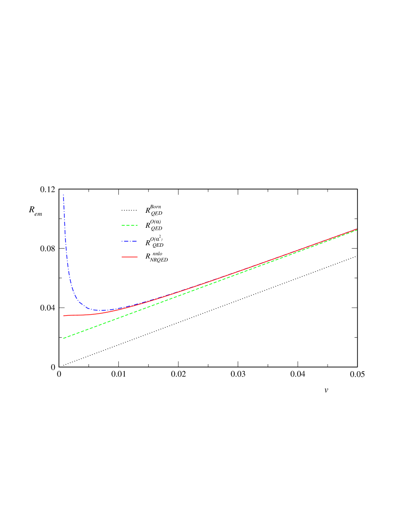
Figure 1: The spectral density $R_{em}$ at low velocities in both QED and NRQED.

The need for performing resummations of the leading non-relativistic terms $\left(\alpha/v\right)^{n}[v,v\alpha,v^{2},\dots]$ is evidenced in Figs. 1 and 2. The spectral density $R_{\mbox{\tiny$em$}}$, calculated in both QED and NRQED, is displayed in Fig. 1 as a function of the $\tau$ velocity. The QED tree-level result vanishes as $v\to 0$, due to the phase space velocity in formula (1), which is cancelled by the first $v^{-1}$ term appearing in the ${\cal O}(\alpha)$ correction, making the cross section at threshold finite. More singular terms near threshold, $v^{-2},v^{-3},\dots$ arising in higher-order corrections completely spoil the expected good convergence of the QED perturbative series in the limit $v\to 0$. This breakdown is clearly seen in the behaviour of the ${\cal O}(\alpha^{2})$ correction to the QED spectral density in Fig. 1. This is no longer the case for the effective theory perturbative series, whose convergence improves as we approach the threshold point, as shown in Fig. 2a, and higher-order corrections reduce the perturbative uncertainty inherent to any series truncated at a finite order. In the whole energy range displayed in Fig. 2a, the differences between the NNLO, NLO and LO results are below 0.8%, which indicates that the LO result, i.e. the Sommerfeld factor, contains the relevant physics to describe the threshold region, although NLO and NNLO corrections would be needed for more accurate descriptions of the total cross section.

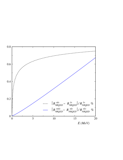
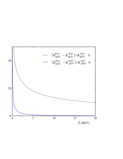
Figure 2: Relative sizes of corrections to $R_{em}(s)$ as calculated in (a) NRQED and (b) QED.

We can safely assume that the NNLO result for the spectral density has a theoretical uncertainty below 0.1% for energies close enough to threshold. At larger energies, the subleading contributions gain importance and the convergence of the double series in $\alpha$ and $v$ is poorer, due to the higher powers of the velocity which are not taken into account. This is the opposite behaviour to that of the usual perturbative QED expansion, Fig. 2b, where the series convergence improves as we move far away the threshold.

Adding the intermediate and initial state corrections we have a complete description of the total cross section of $\tau^{+}\tau^{-}$ production, as shown in Fig. 3. Coulomb interaction between the produced $\tau$’s, governed by the parameter $\alpha/v$, becomes essential right within few MeV above the threshold, and his effects have to be taken into account to all orders in this parameter, making the total cross section finite in this region. Initial state radiation effectively reduces the available center-of-mass energy for $\tau$ production, lowering in this way the total cross section. We can verify that this reduction remains at higher energies above threshold by examining Fig. 4. A maximum energy for the soft photons, $\Delta E=60$ MeV has been chosen to perform the integration (33).

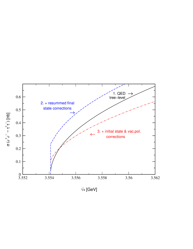
Figure 3: The total cross section $\sigma(e^{+}e^{-}\to\tau^{+}\tau^{-})$ at threshold: at tree level (solid line); plus NNLO corrections to final state interaction, eq. (2) (dashed line); and also including radiative corrections from the initial $e^{+}e^{-}$ state and from vacuum polarization, eq. (4), (dash-dotted curve).

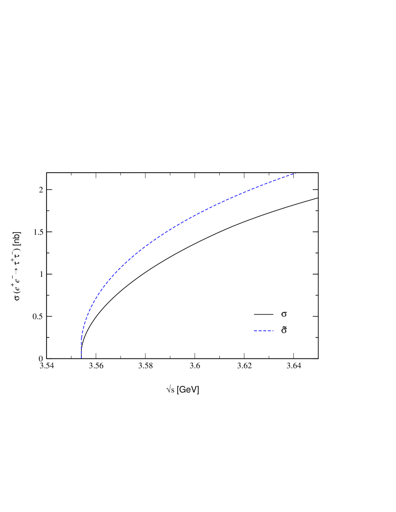
Figure 4: Initial radiation effects in the total cross section $\sigma(e^{+}e^{-}\to\tau^{+}\tau^{-})$ up to energies around 100 MeV above threshold ($v\simeq 0.2$); the dashed line represents $\tilde{\sigma}(e^{+}e^{-}\to\tau^{+}\tau^{-})$, which does not include radiative corrections from initial state, as defined in equation (2).

We should emphasize that NNLO corrections do not modify the predicted behaviour of the LO and NLO cross section as calculated in previous works [8, 9], but are essential to improve the accuracy of experimental fits with higher precision data and, even more important, to guarantee that the truncated perturbative series at NLO gets small corrections from higher-order terms. In this way, we have shown that the theoretical uncertainty of our analysis of $\sigma(e^{+}e^{-}\to\tau^{+}\tau^{-})$ is lower than 0.1%, being the main sources of error our estimates of the hadronic contribution to vacuum polarization and of the initial state radiation. The former could be easily improved using similar techniques to those applied to estimate $\alpha(M_{Z})$, but at the energy point $\sqrt{s}=2m_{\tau}$, including fits to $\sigma(e^{+}e^{-}\to hadrons)$ data, and the latter, being detector dependent, should be accurately monitored and their effects correctly implemented in data analyses. Nevertheless, the statistical uncertainty of the most recent experiments is still much larger than the theoretical one due to low statistics, and we should wait for future machines to improve it.

Acknowledgements

We are grateful to J. Portolés for helpful discussions. We would also like to thank M. Eidemüller, M. Jamin, M. Perrottet and E. de Rafael for useful comments. This work has been supported by the EU TMR, EC-contract No. ERB FMRX-CT98-0169, and by CICYT (Spain) under grant PB97-1261. The work of P. Ruiz-Femenía has been partially supported by a FPU scholarship of the Spanish Ministerio de Educación y Cultura.

Appendix A

The expression of the two-loop spectral density as calculated in perturbative QED and up to NNLO in the velocity expansion ($\tilde{v}\equiv\sqrt{E/M}$) reads [18]:

$$R_{\mbox{\tiny 2loop QED}}^{\mbox{\tiny NNLO}}=\!\!\! \bigg{[} \!\!\!\frac{3}{2}\,\tilde{v}-\frac{17}{16}\,\tilde{v}^{3}\,+{\cal O}(\tilde{v}^{4})\,\bigg{]}+\frac{\alpha(\mu_{\mbox{\tiny$h$}})}{\pi}\,\bigg{[}\,\frac{3\,\pi^{2}}{4}-6\,\tilde{v}+\frac{\pi^{2}}{2}\,\tilde{v}^{2}\,+{\cal O}(\tilde{v}^{3})\,\bigg{]}$$

$$+ \!\!\!\alpha^{2}(\mu_{\mbox{\tiny$h$}})\,\bigg{[}\,\frac{\pi^{2}}{8\,\tilde{v}}+\frac{3}{2}\bigg{(}\,-2\,+n_{f}\,\Big{(}\,\frac{1}{6}\ln\frac{4\,\tilde{v}^{2}\,M^{2}}{\mu_{\mbox{\tiny$hard$}}^{2}}-\frac{5}{18}\,\Big{)}\,\bigg{)}$$

$$+ \!\!\!\bigg{(}\,\frac{49\,\pi^{2}}{192}+\frac{3}{2}\,\kappa-2\,n_{f}\frac{1}{\pi^{2}}\,\,\ln\frac{M^{2}}{\mu_{\mbox{\tiny$hard$}}^{2}}-\,\ln\tilde{v}\,\bigg{)}\,\tilde{v}\,+{\cal O}(\tilde{v}^{2})\,\bigg{]}\,.$$ (A.1)

The constant $\kappa$ has already been defined in eq. (20). The renormalization point in the $\overline{MS}$ scheme has been chosen equal to $\mu_{\mbox{\tiny$hard$}}$, and $M$ denotes the pole mass.

Appendix B

The NRQED Lagrangian relevant for our analysis reads

$${\cal{L}}_{\mbox{\tiny NRQED}}\,=\,\frac{1}{2}\,(\,{\mbox{\boldmath$E$}}^{2}-{\mbox{\boldmath$B$}}^{2}\,)+\,\psi^{\dagger}\,\bigg{[}\,iD_{t}+c_{2}\,\frac{{\mbox{\boldmath$D$}}^{2}}{2\,M}+c_{4}\,\frac{{\mbox{\boldmath$D$}}^{4}}{8\,M^{3}}+\ldots$$ (B.1)

$$\hskip 22.76219pt+\frac{c_{F}\,e}{2\,M}\,{\mbox{\boldmath$\sigma$}}\cdot{\mbox{\boldmath$B$}}+\,\frac{c_{D}\,e}{8\,M^{2}}\,(\,{\mbox{\boldmath$D$}}\cdot{\mbox{\boldmath$E$}}-{\mbox{\boldmath$E$}}\cdot{\mbox{\boldmath$D$}}\,)+\frac{c_{S}\,e}{8\,M^{2}}\,i\,{\mbox{\boldmath$\sigma$}}\,(\,{\mbox{\boldmath$D$}}\times{\mbox{\boldmath$E$}}-{\mbox{\boldmath$E$}}\times{\mbox{\boldmath$D$}}\,)+\ldots\,\bigg{]}\,\psi$$

$$-\,\frac{d_{1}\,e^{2}}{4\,M^{2}}\,(\psi^{\dagger}{\mbox{\boldmath$\sigma$}}\sigma_{2}\chi^{*})\,(\chi^{T}\sigma_{2}{\mbox{\boldmath$\sigma$}}\psi)-\,\frac{d_{2}}{M^{2}}\,(\psi^{\dagger}\sigma_{2}\chi^{*})\,(\chi^{T}\sigma_{2}\psi)\,+\,$$

$$+\frac{d_{3}\,e^{2}}{6\,M^{4}}\,\Big{[}\,(\psi^{\dagger}{\mbox{\boldmath$\sigma$}}\sigma_{2}\chi^{*})\,(\chi^{T}\sigma_{2}{\mbox{\boldmath$\sigma$}}(-\mbox{$\frac{i}{2}$}{\stackrel{{\scriptstyle\leftrightarrow}}{{\mbox{\boldmath$D$}}}})^{2}\psi)+\mbox{h.c.}\,\Big{]}+\ldots\,\,.$$

The lepton and antilepton are described by the Pauli spinors $\psi$ and $\chi$, respectively. Antilepton bilinears and higher–order operators have been omitted. The first line in eq. (B.1) is related to the kinetic term of the QED Lagrangian, with the bilinear $\psi$ terms coming from the expansion of the lepton relativistic energy up to ${\cal O}(1/M^{3})$. Second line terms reproduce the electromagnetic couplings of the leptons with photons of energy lower than $M$. Four fermion operators displayed in latter lines reproduce production and annihilation of an $\ell^{+}\ell^{-}$ pair in a S-wave singlet ($d_{2}$) or triplet ($d_{1}$ and $d_{3}$) state. Additional interaction terms between photon fields should be introduced to simulate fermion loops. The short-distance coefficients $c_{i},d_{i}$ must be determined following the matching procedure up to a certain order in $\alpha$, in order to absorb infinities arising in calculations beyond tree level.

Which interactions are to be kept for a given precision (in $\alpha$ and $v\sim p/M$) is dictated by counting rules. The presence of two dynamical scales in the theory, the fermions three-momentum $\simeq Mv$, and their kinetic energies $\simeq Mv^{2}$, makes the NRQED counting rules more involved than in most effective field theories. While the factors of $\alpha$ in a specific diagram can be read off from vertex coefficients, powers of $v$ are also generated by internal propagators and loop integrations. There has been a hard discussion during recent years on how to organize calculations within NRQED/NRQCD in a systematic expansion in $v$ [39], especially in the context of dimensional regularization. The situation seems to be clarified with the new formulation proposed in Refs. [40, 41]. In a cutoff scheme power counting rules for the velocity had been previously derived by Labelle [20] using time ordered perturbation theory together with the Coulomb gauge to separate the “soft” photons (with energy $E_{\gamma}\simeq Mv$) from the “ultrasoft” ones ($E_{\gamma}\simeq Mv^{2}$). Although quite troublesome for calculations beyond NNLO in the velocity expansion, these rules give the order in $v$ of diagrams containing only soft photons by simple dimensional analysis. Following these rules one proves that the latter diagrams are all we need to describe low-energy interaction between the pair of fermions up to NNLO. Moreover, soft photons have an energy independent propagator and therefore all interactions up to NNLO can be described in terms of potentials, being this a highly non-trivial result which cannot be derived in the context of full QED covariant perturbation theory .

The effective $\gamma\tau^{+}\tau^{-}$ coupling seen by the non-relativistic leptons is given by the expansion of the QED current in terms of the operators of the low-energy theory:

$$j^{k}_{\mbox{\tiny NR}}(x)=b_{1}\,\Big{(}\psi^{\dagger}\sigma^{k}\chi\Big{)}(x)-\frac{b_{2}}{6M^{2}}\,\Big{(}{\psi}^{\dagger}\sigma^{k}(\mbox{$-\frac{i}{2}$}\stackrel{{\scriptstyle\leftrightarrow}}{{\mbox{\boldmath$D$}}})^{2}\chi\Big{)}(x)+\ldots\,.$$ (B.2)

We have only quoted the terms which are needed at NNLO. The first piece is a dimension-three current while the second has dimension-five and it is already of NNLO, as dictated by counting rules [20] due to the presence of the $1/M^{2}$ factor. Notice that both pieces have quantum numbers ${}^{3}S_{1}$. There is another dimension five current, describing ${}^{3}D_{1}$ $\tau^{+}\tau^{-}$ production which however would not contribute to the NNLO cross section because the correlator of the product of a ${}^{3}S_{1}$ current and a ${}^{3}D_{1}$ one vanishes. The Wilson coefficients of the NRQED ${}^{3}S_{1}$ current encode the effects of the hard modes which have been integrated out. The coefficient $b_{1}$ needs to be known at order $\alpha^{2}$, while $b_{2}=1$ at NNLO. Inserting expansion (B.2) into the correlation function (6) leads to the NRQED expression of the ratio $R_{\mbox{\tiny$em$}}$ at NNLO

$$R^{\mbox{\tiny NNLO}}_{\mbox{\tiny$em$}}(q^{2})=\frac{4\,\pi}{q^{2}}\,\mbox{Im}\Big{(}C_{1}\,\Big{[}\,{\cal{A}}_{1}(E)\,\Big{]}-\frac{1}{6M^{2}}C_{2}\,\Big{[}\,{\cal{A}}_{2}(E)\,\Big{]}\Big{)}\,,$$ (B.3)

where

$${\cal{A}}_{1} = -i\int d^{4}x\,e^{iqx}\,\Big{\langle}\,0\,\Big{|}T\,\Big{(}{\psi}^{\dagger}{\mbox{\boldmath$\sigma$}}\,\chi\cdot{\chi}^{\dagger}{\mbox{\boldmath$\sigma$}}\,\psi\Big{)}\,\Big{|}\,0\,\Big{\rangle}\,,$$ (B.4)

$${\cal{A}}_{2} = -i\int d^{4}x\,e^{iqx}\,\Big{\langle}\,0\,\Big{|}T\,\Big{(}{\psi}^{\dagger}{\mbox{\boldmath$\sigma$}}\,\chi\cdot{\chi}^{\dagger}{\mbox{\boldmath$\sigma$}}\,(\mbox{$-\frac{i}{2}$}\stackrel{{\scriptstyle\leftrightarrow}}{{\mbox{\boldmath$D$}}})^{2}\psi+\mbox{h.c.}\Big{)}\,\Big{|}\,0\,\Big{\rangle}\,.$$ (B.5)

The short distance coefficients read $C_{1}=(b_{1})^{2}$ and $C_{2}=1$. The correlators ${\cal{A}}_{1}$ and ${\cal{A}}_{2}$ contain the non-relativistic interactions derived from the NRQED Lagrangian. Such interactions, at NNLO, are purely described by instantaneous potentials, similar to those used in familiar quantum mechanics. Therefore, once the lepton pair is created by the external current with relative momentum $k$ and until it is annihilated, the four point function describing their evolution reduces to a Schrödinger Green function for a two-body system with kinetic energy $E=\sqrt{s}-2M$, see Fig. 5.

Figure 5: Graphical representation of the NRQED vector-current correlator diagrams: the lepton pair $\ell^{+}\ell^{-}$ is created and annihilated by the coupling ${\psi}^{\dagger}{\mbox{\boldmath$\sigma$}}\,\chi$ in (B.4), and all the intermediate diagrams of the $\ell^{+}\ell^{-}$ non-relativistic NNLO interaction are resummed in the Green’s function $G(E)$.

The exact relation for ${\cal{A}}_{1}$ reads

$${\cal{A}}_{1}(E) = \mbox{Tr}\int\frac{d^{3}\mbox{\boldmath$k$}}{(2\pi)^{3}}\int\frac{d^{3}\mbox{\boldmath$k$}^{\prime}}{(2\pi)^{3}}\,\mbox{\boldmath$\sigma$}\,\tilde{G}({\mbox{\boldmath$k$}},{\mbox{\boldmath$k$}^{\prime}};E)\,\mbox{\boldmath$\sigma$}$$ (B.6)

$$= 6\,\Bigl{[}\,\lim_{r,r^{\prime}\to 0}\,G({\mbox{\boldmath$r$}},{\mbox{\boldmath$r$}^{\prime}};E)\,\Bigr{]}\,,$$

where we have used the identity $\mbox{Tr}(\mbox{\boldmath$\sigma$}\cdot\mbox{\boldmath$\sigma$})=3\,\mbox{Tr}(\mbox{I})=6$. One can check that eq. (B.6) gives the right proportionality factor between ${\cal{A}}_{1}$ and $G$ just considering the free case. There is no extra factor coming from the different normalizations of the relativistic and the non-relativistic quantities.

For the ${\cal{A}}_{2}$ correlator we have

$${\cal{A}}_{2}(E) = \mbox{Tr}\int\frac{d^{3}\mbox{\boldmath$k$}}{(2\pi)^{3}}\int\frac{d^{3}\mbox{\boldmath$k$}^{\prime}}{(2\pi)^{3}}\,({\mbox{\boldmath$k$}}^{2}+{\mbox{\boldmath$k$}^{\prime}}^{2})\,\tilde{G_{c}}({\mbox{\boldmath$k$}},{\mbox{\boldmath$k$}^{\prime}};E)\,$$ (B.7)

$$= -6\left({\mbox{\boldmath$\nabla$}}^{2}_{r}+{\mbox{\boldmath$\nabla$}}^{2}_{r^{\prime}}\right)G_{c}({\mbox{\boldmath$r$}},{\mbox{\boldmath$r$}^{\prime}};E)|_{r,r^{\prime}\to 0}\,.$$

As ${\cal{A}}_{2}$ is already of NNLO, only the Green’s function for the Coulomb potential shall be considered. Relation (B.7) can be further simplified by using the Schrödinger eq. (15), retaining just the LO piece of $V_{c}(r)$. For the imaginary part, we have

$$-\frac{{\mbox{\boldmath$\nabla$}}^{2}_{r}}{M}\,\mbox{Im}\,G_{c}({\mbox{\boldmath$r$}},{\mbox{\boldmath$r$}^{\prime}};E)\,=\,\left(E-V_{c}^{\mbox{\tiny LO}}(r)\,\right)\,\mbox{Im}\,G_{c}({\mbox{\boldmath$r$}},{\mbox{\boldmath$r$}^{\prime}};E)\,=\,\left(E+\frac{\alpha}{r}\,\right)\,\mbox{Im}\,G_{c}({\mbox{\boldmath$r$}},{\mbox{\boldmath$r$}^{\prime}};E)\,.$$ (B.8)

In the limit $r,r^{\prime}\to 0$, the term $\alpha/r\,\mbox{Im}G_{c}$ represents an ultraviolet divergence which must be regularized. Following the direct matching procedure [27] to fix the value of the short distance coefficient $C_{1}$ allows us to drop power-like divergences, such as $\alpha/r\,\mbox{Im}G_{c}|_{r\to 0}$, which must cancel with similar ultraviolet divergences in $C_{1}$ in the final expression for the total cross section. Therefore we can safely substitute $\mbox{Im}\,{\cal{A}}_{2}$ by $12EM\,G_{c}({\mbox{\boldmath$r$}},{\mbox{\boldmath$r$}^{\prime}};E)|_{r,r^{\prime}\to 0}$ in (B.3) to get the complete relation between the spectral density at NNLO and the non-relativistic Green’s functions:

$$R^{\mbox{\tiny NNLO}}_{\mbox{\tiny$em$}}(q^{2})=\frac{6\,\pi}{M^{2}}\,\mbox{Im}\Big{(}C_{1}\,G({\mbox{\boldmath$0$}},{\mbox{\boldmath$0$}};E)\,-\frac{4E}{3M}\,G_{c}({\mbox{\boldmath$0$}},{\mbox{\boldmath$0$}};E)\Big{)}\,,$$ (B.9)

where we have expanded the relation $q^{2}=(2M+E)^{2}$ to first order in $E/2M$, which is already a NNLO contribution.

Appendix C

The well-known Coulomb Green’s function [42], solution of the LO Hamiltonian, at the origin reads ($\tilde{v}\equiv\sqrt{E/M}\,$)

$$G_{c}^{r}({\mbox{\boldmath$0$}},{\mbox{\boldmath$0$}};E)\,=\,\frac{M^{2}}{4\pi}\,\bigg{(}\,i\,\tilde{v}-\alpha(\mu_{s})\bigg{[}{\mbox{ln}}\,\Big{(}-i\frac{M\tilde{v}}{\mu_{\mbox{\tiny$fac$}}}\Big{)}+\gamma+{\Psi}\Big{(}1-i\,\frac{\alpha(\mu_{s})}{2\,\tilde{v}}\Big{)}\,\bigg{]}\bigg{)}\,,$$ (C.1)

where $\Psi(z)=\frac{d}{dz}\log\Gamma(z)$ and $\Gamma(z)$ is the Euler Gamma function. The superscript ‘r’ stands for ‘renormalized’, since in the short distance limit $r,r^{\prime}\to 0$ the Coulomb Green’s function, and some of the $\delta G$, have $1/r$ and $\log(r)$ divergent terms. Following the lines of previous papers [22, 43] power-like divergences are subtracted and ultraviolet log-terms are regularized by introducing a cutoff $\mu_{f}$ and hence subtracting the energy-independent part. However, the imaginary part of $G_{c}$ has no ultraviolet divergent terms, so they would not contribute to the total cross section. This is not longer the case for the corrections $\delta_{\mbox{\tiny Ki,BF}}G$ and $\delta_{\mbox{\tiny An}}G$, and their (imaginary part) residual dependence on the $\mu_{f}$-scale will be canceled with the scale dependence of the coefficient $C_{1}$, which is determined using the “direct matching procedure” [27] described at the end of section 3. We quote the result for $\delta_{\mbox{\tiny Ki,BF}}G$ ($C_{F}\to 1,T_{F}\to 1$ and $C_{A}\to 0$ for the U(1) group) [22]:

$$\delta_{\mbox{\tiny Ki,BF}}G(0,0;E) = \frac{\alpha(\mu_{s})M^{2}}{4\pi}\,\Bigg{(}i\,{5\over 8}\,\frac{\tilde{v}^{3}}{\alpha(\mu_{s})}-2\tilde{v}^{2}\left[\ln\left(-i\frac{M\tilde{v}}{\mu_{\mbox{\tiny$fac$}}}\right)+\gamma+\Psi\left(1-i\frac{\alpha(\mu_{s})}{2\tilde{v}}\right)\right]$$ (C.2)

$$+\,\,\,i\,{11\over 16}\alpha(\mu_{s})\tilde{v}\,\Psi^{\prime}\left(1-i{\alpha(\mu_{s})\over 2\tilde{v}}\,\right)\Bigg{)}+{4\pi\over 3}{\alpha(\mu_{s})\over M^{2}}G_{c}^{r}(0,0,E)^{2}\,.$$

The integration for the $V_{\mbox{\tiny An}}$ potential is trivial, and the resulting (renormalized) correction $\delta_{\mbox{\tiny An}}G$ reads

$$\delta_{\mbox{\tiny An}}G(0,0;E)=-2{\alpha(\mu_{s})\pi\over M^{2}}G_{c}^{r}(0,0,E)^{2}\,.$$ (C.3)

The ${\cal O}(\alpha)$ correction to the Coulomb potential, $V_{c}^{\tiny(1)}(r)$, must be iterated twice because it is a NLO contribution. The corresponding corrections $\delta^{\mbox{\tiny NLO}}_{\tiny 1}G$ and $\delta^{\mbox{\tiny NNLO}}_{\tiny 1}G$ have been calculated in [13] and [26], respectively. The details of their calculation can be found therein. Their final expressions read:

$$\delta^{\mbox{\tiny NLO}}_{1}G(0,0;E)=\bigg{(}\frac{\alpha(\mu_{s})}{4\pi}\bigg{)}^{2}M^{2}\left\{\sum_{m=0}^{\infty}F^{2}(m)(m+1)\left(C_{0}^{1}+(L(v)+\Psi(m+2))C_{1}^{1}\right)\right.$$

$$-2\sum_{m=1}^{\infty}\sum_{n=0}^{m-1}F(m)F(n){n+1\over m-n}C_{1}^{1}+2\sum_{m=0}^{\infty}F(m)\left(C_{0}^{1}+(L(v)-2\gamma-\Psi(m+1))C_{1}^{1}\right)$$

$$\left.+L(v)C_{0}^{1}+\left(-\gamma L(v)+{1\over 2}L(v)^{2}\right)C_{1}^{1}\right\}\,,$$ (C.4)

and

$$\delta^{\mbox{\tiny NNLO}}_{1}G(0,0;E)=i\left({\alpha(\mu_{s})\over 4\pi}\right)^{2}{\alpha(\mu_{s})^{2}\over 4\pi}{M^{2}\over 2v}\left\{\sum_{m=0}^{\infty}H^{3}(m)(m+1)\right.\cdot$$

$$\cdot\left(C_{0}^{1}+\left(\Psi(m+2)+L(v)\right)C_{1}^{1}\right)^{2}$$

$$-2\sum_{m=1}^{\infty}\sum_{n=0}^{m-1}{n+1\over m-n}C_{1}^{1}\left(H^{2}(m)H(n)\left(C_{0}^{1}+\left(\Psi(m+2)+L(v)-{1\over 2}{1\over m-n}\right)C_{1}^{1}\right)\right.$$

$$\left.+H(m)H^{2}(n)\left(C_{0}^{1}+\left(\Psi(n+2)+L(v)-{1\over 2}{n+1\over(m-n)(m+1)}\right)C_{1}^{1}\right)\right)$$ (C.5)

$$+2(C_{1}^{1})^{2}\left(\sum_{m=2}^{\infty}\sum_{l=1}^{m-1}\sum_{n=0}^{l-1}{H(m)H(n)H(l)}{n+1\over(l-n)(m-n)}\right.$$

$$+\sum_{m=2}^{\infty}\sum_{n=1}^{m-1}\sum_{l=0}^{n-1}{H(m)H(n)H(l)}{l+1\over(n-l)(m-n)}$$

$$\left.\left.+\sum_{n=2}^{\infty}\sum_{m=1}^{n-1}\sum_{l=0}^{m-1}{H(m)H(n)H(l)}{(l+1)(m+1)\over(n+1)(n-l)(n-m)}\right)\right\}\,,$$

with

$$F(m)=\frac{i}{2(m+1)}\,\frac{\alpha(\mu_{s})}{v}\,\bigg{(}m+1-i\,\frac{\alpha(\mu_{s})}{2v}\bigg{)}^{-1}\,,$$ (C.6)

$$L(v)=-{\mbox{ln}}\bigg{(}-2i\frac{Mv}{\mu_{s}}\bigg{)}\,,$$ (C.7)

and finally

$$H(m)=\left(m+1-i{\displaystyle{\alpha(\mu_{s})\over 2v}}\right)^{-1}.$$

The constants $C_{0}^{1}$, $C_{1}^{1}$ are defined in terms of $\beta_{1}$ (14):

$$C_{0}^{1} = a_{1}+2\beta_{1}\gamma\,,$$

$$C_{1}^{1} = 2\beta_{1}\,.$$ (C.8)

The iteration of the ${\cal O}(\alpha^{2})$ piece, $V_{c}^{\tiny(2)}(r)$, was also computed in [13]:

$$\delta_{2}G(0,0;E)=\left({\alpha(\mu_{s})\over 4\pi}\right)^{2}{\alpha(\mu_{s})M^{2}\over 4\pi}\left\{\sum_{m=0}^{\infty}F^{2}(m)\left((m+1)\left(C_{0}^{2}+L(v)C_{1}^{2}+L^{2}(k)C_{2}^{2}\right)\right.\right.$$

$$\left.+(m+1)\Psi(m+2)\left(C_{1}^{2}+2L(v)C_{2}^{2}\right)+I(m)C_{2}^{2}\right)$$

$$+2\sum_{m=1}^{\infty}\sum_{n=0}^{m-1}F(m)F(n)\left(-{n+1\over m-n}\left(C_{1}^{2}+2L(v)C_{2}^{2}\right)+J(m,n)C_{2}^{2}\right)$$ (C.9)

$$+2\sum_{m=0}^{\infty}F(m)\left(C_{0}^{2}+L(v)C_{1}^{2}+(L^{2}(v)+K(m))C_{2}^{2}-(2\gamma+\Psi(m+1))\left(C_{1}^{2}+2L(v)C_{2}^{2}\right)\right)$$

$$\left.+L(v)C_{0}^{2}+\left(-\gamma L(v)+{1\over 2}L^{2}(v)\right)C_{1}^{2}+N(v)C_{2}^{2}\right\}\,,$$

with the functions $I(m),J(m,n),K(m),N(v)$ defined as

$$I(m)=(m+1)\left(\Psi^{2}(m+2)-\Psi^{\prime}(m+2)+{\pi^{2}\over 3}-{2\over(m+1)^{2}}\right)$$

$$-2(\Psi(m+1)+\gamma),$$

$$J(m,n)=2{n+1\over m-n}\left(\Psi_{1}(m-n)-{1\over n+1}+2\gamma\right)$$

$$+2{m+1\over m-n}(\Psi(m-n+1)-\Psi(m+1)),$$

$$K(m)=2(\Psi(m+1)+\gamma)^{2}+\Psi^{\prime}(m+1)-\Psi^{2}(m+1)+2\gamma^{2},$$

$$N(v)=\left(\gamma+{\pi^{2}\over 6}\right)L(v)-\gamma L^{2}(v)+{1\over 3}L^{3}(v)\,,$$

and the constants

$$C_{0}^{2}=\Big{(}\frac{\pi^{2}}{3}+4\gamma^{2}\Big{)}+\beta_{1}^{2}+2(\beta_{2}+2\beta_{1}a_{1})\gamma+a_{2}\,,$$

$$C_{1}^{2}=2(\beta_{2}+2\beta_{1}a_{1})+8\beta_{1}^{2}\gamma\,,$$

$$C_{2}^{2}=4\beta_{1}^{2}\,.$$

None of the above mentioned Coulomb $\delta G$ corrections have energy dependent ultraviolet terms on their imaginary part, so no matching is necessary for them.

References

• [1] J. Kirkby, A $\tau$–Charm Factory at CERN, CERN-EP/87-210 (1987).
• [2] J.M. Jowett, Initial Design of a $\tau$–Charm Factory at CERN CERN LEP-TH/87-56 (1987); The $\tau$–Charm Factory Storage Ring, CERN LEP-TH/88-22 (1988).
• [3] Proc. Tau–Charm Factory Workshop (SLAC, California, 1989), ed. L.V. Beers, SLAC-Report-343 (1989).
• [4] Proc. 3rd Workshop on the Tau-Charm Factory (Marbella, Spain, 1993), eds. J. Kirkby and R. Kirkby (Editions Frontières, Gif-sur-Yvette, 1994).
• [5] Workshop on Prospects for CLEO/CESR with $3<E_{\mbox{\tiny CM}}<5$ GeV, Cornell, May 2001.
• [6] A. Pich, Perspectives on Tau–Charm Factory Physics, in [4] p. 767.
• [7] J.Z. Bai et al (BES), Phys. Rev. D53 (1996) 20.
• [8] M.B. Voloshin, Topics in Tau Physics at a Tau-Charm Factory, TPI-MINN-89/33-T (1989), unpublished [hep-ph/9312358].
• [9] M. Perrottet, An Improved Calculation of $\sigma(e^{+}\,e^{-}\to\tau^{+}\,\tau^{-})$ Near Threshold, in [4] p. 89.
• [10] B.H. Smith and M.B. Voloshin, Phys. Lett. B324 (1994) 117.
• [11] W. E. Caswell and G. P. Lepage, Phys. Lett. B167 (1986) 437.
• [12] M. Jamin and A. Pich, Nucl. Phys. B507 (1997) 334.
• [13] J. H. Kühn, A. A. Penin and A. A. Pivovarov, Nucl. Phys. B534 (1998) 356.
• [14] K. Melnikov and A. Yelkhovsky, Phys. Rev. D59 (1999) 114009;
A.A. Penin and A.A. Pivovarov, Nucl. Phys. B549 (1999) 217;
M. Beneke and A. Signer, Phys. Lett. B471 (1999) 233;
A.H. Hoang, Phys. Rev. D59 (1999) 014039.
• [15] A.H. Hoang et al., Eur. Phys. J. direct C3, (2000) 1.
• [16] R. Barbieri, J.A. Mignaco and E. Remiddi, Nuovo Cimento 11A (1972) 824.
• [17] E.A. Kuraev and V.S. Fadin, Yad. Fiz. 41 (1985) 733 [Sov. J. Nucl. Phys. 41 (1985) 466].
• [18] A.H. Hoang, Phys. Rev. D56 (1997) 7276.
• [19] A. Sommerfeld, Atombau und Spektrallinien, Vol.II, Vieweg, Braunschweig, 1939.
• [20] P. Labelle, Phys. Rev. D58 (1998) 093913.
• [21] F.A. Berends, K.J.F. Gaemers and R. Gastmans, Nucl. Phys. B57 (1973) 381.
• [22] A. H. Hoang and T. Teubner, Phys. Rev. D58 (1998) 114023.
• [23] W. Fischler, Nucl. Phys. B129 (1977) 157 ;
A. Billoire, Phys. Lett. B92 (1980) 343.
• [24] M. Peter, Nucl. Phys. B501 (1997) 471;
Y. Schröder, Phys. Lett. B447 (1999) 321.
• [25] L. D. Landau and E. M. Lifshitz, Relativistic Quantum Theory, Part 1 (Pergamos, Oxford, 1974)
• [26] A. A. Penin and A. A. Pivovarov, Phys. Lett. B435 (1998) 413.
• [27] A.H. Hoang, Phys. Rev. D57 (1998) 1615.
• [28] G. Källen and A. Sabry, Kgl. Danske Videnskab. Selskab Mat. Fys. Medd. 29 (1955) No.17.
• [29] F. Guerrero and A. Pich, Phys. Lett. B412 (1997) 382.
• [30] G.Ecker, J. Gasser, A. Pich and E. de Rafael, Nucl. Phys. B321 (1989) 311;
G.Ecker, J. Gasser, H. Leutwyler, A. Pich and E. de Rafael, Phys. Lett. B223 (1989) 425.
• [31] D. Gómez-Dumm, A. Pich and J. Portolés, Phys. Rev. D62 (2000) 054014.
• [32] S. Eidelman and F. Jegerlehner, Z. Phys. C67 (1995) 585.
• [33] M. Davier and A. Höcker, Phys. Lett. B435 (1998) 427.
• [34] A. Pich and J. Portolés, The vector form-factor of the pion from unitariry and analyticity: a model independent approach, hep-ph/0101194.
• [35] A.A. Penin and A.A. Pivovarov, Analytical results for $e^{+}e^{-}\to\bar{t}t$ and $\gamma\gamma\to\bar{t}t$ observables near the threshold up to the next-to-next-to leading order of NRQCD, hep-ph/9904278.
• [36] A.H. Hoang and T. Teubner, Phys. Rev. D60 (1999) 114027.
• [37] Particle Data Group, Review of Particle Properties, Eur. Phys. J.  C15 (2000) 1.
• [38] A. Pich,Tau Physics: Theoretical Perspective, hep-ph/0012297;
Tau Physics, Proc. 19th Int. Symposium on Lepton and Photon Interactions at High Energies (Stanford, 1999), eds. J. Jaros and M. Peskin (World Scientific, Singapore, 2000) 157.
• [39] M.E. Luke and A.V. Manohar, Phys. Rev. D55 (1997) 4129;
A.V. Manohar, Phys. Rev. D56 (1997) 230;
A. Pineda and J. Soto, Nucl. Phys. Proc. Suppl. 64 (1998) 428;
M. Beneke and V.A. Smirnov, Nucl. Phys. B522 (1998) 321;
H.W. Griesshammer, Phys. Rev. D58 (1998) 094027.
• [40] M.E. Luke, A.V. Manohar and I.Z. Rothstein, Phys. Rev. D61 (2000) 074025.
• [41] A.V. Manohar, J. Soto, I.W. Stewart, Phys.Lett. B486 (2000) 400.
• [42] E.H. Wichmann and C. H. Woo, J. Math. Phys. 2 (1961) 178;
L. Hostler, J. Math. Phys. 5 (1964) 591;
J. Schwinger, J. Math. Phys. 5 (1964) 1606.
• [43] K. Melnikov and A. Yelkhovsky, Nucl. Phys. B528 (1998) 59.