1 Introduction

Solar parameters in the range of the large mixing angle MSW solution (LMA-MSW)[1, 2] are expected to affect sizeably the neutrino oscillation[3] probabilities at terrestial distances. The discovery of CP-violation in the lepton sector might then be at reach [4]-[17].

Consider a neutrino factory from a muon storage ring [18, 19] with muon energies of some dozens of GeV. In [11] a detailed study of the potential of such a neutrino factory in determining the leptonic CP-violating phase, $\delta$, and the angle $\theta_{13}$ was performed, within the LMA-MSW. Just the range $0<\delta<90^{\circ}$ and $\theta_{13}>1^{\circ}$ was analyzed, though. It has been argued that the CP phase can be only determined up to a sign [17]. In order to clarify this issue the full range $-180^{\circ}<\delta<180^{\circ}$ has to be explored. Besides, it is important to understand what is the lower value of $\theta_{13}$ at which the sensitivity to CP violation is lost.

A second limitation of the analysis performed in [11] is that the atmospheric parameters, $\theta_{23}$ and $\Delta m^{2}_{23}$, as well as the solar ones, $\theta_{12}$ and $\Delta m^{2}_{12}$, were assumed to be known. Neither an error estimate on the average Earth matter density was included. It has been recently pointed out [20] that the errors in these parameters might modify drastically the conclusions reached in [11].

For the atmospheric parameters, the main source of new information will come from proposed long baseline accelarator experiments (KEK, Minos, Opera)[21] while for the solar ones lying in the LMA-MSW range, mostly from Kamland[22]. Minos is expected to measure $\sin^{2}2\theta_{23}$ and $\Delta m^{2}_{23}$ at the $10\%$ level [23], in the range allowed by SuperKamiokande [24]. In the neutrino factory this uncertainty is expected to be improved to about $1\%$ from muon disappearance measurements[25, 26, 13]. Concerning the solar parameters in the LMA-MSW regime, $\sin^{2}2\theta_{12}$ and $\Delta m_{12}^{2}$, Kamland will be able to determine them to better than $10\%$ for $\Delta m^{2}_{12}\geq 10^{-5}$ eV² and $\sin^{2}2\theta_{12}>0.7$ [27], well before the time of the neutrino factory.

In this work we study, by means of an approximate analytical formula, the existence of degenerate solutions for the parameters ($\mbox{$\theta_{13}$},\delta$): solutions that give the same probabilities for the $\nu_{e}\nu_{\mu}$ and ${\bar{\nu}}_{e}{\bar{\nu}}_{\mu}$ transitions than the one chosen by nature. We complete the analysis of [11] by considering the full range of $\theta_{13}$ and $\delta$, which reveals the existence of these degeneracies, and include the errors with which the atmospheric and solar parameters will be known at the time of the neutrino factory. Furthermore, we discuss the uncertainty on the average Earth electron density along the neutrino path, and study its relevance in the range $O(1$–$10\%)$.

In section 2, we analyse the sensitivity to CP violation in the full range $-180^{\circ}<\delta<180^{\circ}$ and clarify the correlation of $\delta$ with the unknown parameter $\theta_{13}$. In section 3, the results of ref. [11] on the simultaneous fits to $\theta_{13}$ and $\delta$ are extended to the full range of $\delta$ and $\theta_{13}<1^{\circ}$. Section 4 describes the method to include in the analysis the errors on the atmospheric and solar parameters and on the Earth matter density, taking properly into account the corresponding correlations between neutrinos and antineutrinos, as well as between different energy bins and baselines (when more than one baseline is considered). The results of the fits including these errors and the discussion of the relative importance of each of them are then presented. Section 5 states our conclusions.

2 Sensitivity to CP violation

Given the high intensity expected at the neutrino factory, the effects of the solar mass difference, $\Delta m^{2}_{12}$, are not negligible over terrestrial distances in the LMA-MSW scenario, opening the way to observing leptonic CP violation.

The best way to measure $\delta$ and $\theta_{13}$ is through the subleading transitions $\nu_{e}\rightarrow\nu_{\mu}$ and ${\bar{\nu}}_{e}\rightarrow\bar{\nu}_{\mu}$. They can be measured at a neutrino factory by searching for wrong–sign muons [19, 5] while running in both polarities of the beam, i.e. $\mu^{+}$ and $\mu^{-}$ respectively.

The exact oscillation probabilities in matter when no mass difference is neglected have been derived analytically in [28]. However, the physical implications of the formulae in [28] are not easily derived. Defining $\Delta_{ij}\equiv\frac{\Delta m^{2}_{ij}}{2E}$, a convenient and precise approximation is obtained by expanding to second order in the following small parameters: $\theta_{13}$, $\Delta_{12}/\mbox{$\Delta_{23}$}$, $\Delta_{12}/A$ and $\Delta_{12}\,L$. The result is (details of the calculation can be found in [11]):

$$P_{\nu_{e}\nu_{\mu}(\bar{\nu}_{e}\bar{\nu}_{\mu})} = s_{23}^{2}\sin^{2}2\mbox{$\theta_{13}$}\,\left(\frac{\mbox{$\Delta_{13}$}}{\tilde{B}_{\mp}}\right)^{2}\,\sin^{2}\left(\frac{\tilde{B}_{\mp}\,L}{2}\right)\,+\,c_{23}^{2}\sin^{2}2\theta_{12}\,\left(\frac{\Delta_{12}}{A}\right)^{2}\,\sin^{2}\left(\frac{A\,L}{2}\right)$$ (1)

$$+ \tilde{J}\;\frac{\Delta_{12}}{A}\,\frac{\mbox{$\Delta_{13}$}}{\tilde{B}_{\mp}}\,\sin\left(\frac{AL}{2}\right)\,\sin\left(\frac{\tilde{B}_{\mp}L}{2}\right)\,\cos\left(\pm\delta-\frac{\mbox{$\Delta_{13}$}\,L}{2}\right)\,,$$

where $L$ is the baseline, $\tilde{B}_{\mp}\equiv|A\mp\mbox{$\Delta_{13}$}|$ and the matter parameter, $A$, is given in terms of the average electron number density, $n_{e}(L)$, as $A\equiv\sqrt{2}\,G_{F}\,n_{e}(L)$, where the $L$-dependence will be taken from [29]. $\tilde{J}$ is defined as

$$\tilde{J}\equiv\cos\theta_{13}\;\sin 2\theta_{13}\;\sin 2\theta_{23}\;\sin 2\theta_{12}.$$ (2)

In the limit $A\rightarrow 0$, this expression reduces to the simple formulae in vacuum

$$P_{\nu_{e}\nu_{\mu}(\bar{\nu}_{e}\bar{\nu}_{\mu})} = s_{23}^{2}\,\sin^{2}2\mbox{$\theta_{13}$}\,\sin^{2}\left(\frac{\mbox{$\Delta_{13}$}\,L}{2}\right)+c_{23}^{2}\,\sin^{2}2\theta_{12}\,\sin^{2}\left(\frac{\Delta_{12}\,L}{2}\right)$$ (3)

$$+ \tilde{J}\,\cos\left(\pm\delta-\frac{\mbox{$\Delta_{13}$}\,L}{2}\right)\;\frac{\Delta_{12}\,L}{2}\sin\left(\frac{\mbox{$\Delta_{13}$}\,L}{2}\right).$$

In the following we will denote by atmospheric, $P^{atm}_{\nu(\bar{\nu})}$, solar, $P^{sol}$, and interference term, $P^{inter}_{\nu(\bar{\nu})}$, the three terms in eqs. (1).

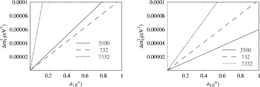
Figure 1: Contours $P^{atm}_{\nu}=P^{sol}$ (left) and $P^{atm}_{\bar{\nu}}=P^{sol}$ (right) on the plane $\theta_{13},\Delta m_{12}^{2}$, for the three reference baselines. $\Delta m_{23}^{2}=3\times 10^{-3}$ eV² and $\theta_{12}=\theta_{23}=45^{\circ}$.

It is easy to show that

$$|P^{inter}_{\nu(\bar{\nu})}|\leq P^{atm}_{\nu(\bar{\nu})}+P^{sol},$$ (4)

implying two very different regimes. When $\theta_{13}$ is relatively large or $\Delta m^{2}_{12}$ small, the probability is dominated by the atmospheric term, since $P^{atm}_{\nu(\bar{\nu})}\gg P^{sol}$. We will refer to this situation as the atmospheric regime. Conversely, when $\theta_{13}$ is very small or $\Delta m^{2}_{12}$ large, the solar term dominates $P^{sol}\gg P^{atm}_{\nu(\bar{\nu})}$. This is the solar regime. Fig. 1 illustrates the separation between the two regimes on the plane $\Delta m^{2}_{12}$ and $\theta_{13}$ for neutrinos and antineutrinos, as derived from eq. (1). The area to the right(left) of the curves corresponds to the atmospheric(solar) regime.

We discuss next the subtleties in the measurent of CP violation in both regimes.

2.1 Correlation between $\delta$ and $\theta_{13}$

The oscillation probabilities of eq. (1), from whose measurement $\delta$ could be extracted, depend as well on $\theta_{23},\Delta m^{2}_{23},\theta_{12},\Delta m^{2}_{12},A$ and $\theta_{13}$. Uncertainties in the latter quantities can then hide the effect of CP violation. Although the first five of these parameters are expected to be known at the time of the neutrino factory with a good accuracy, $\theta_{13}$ might well remain unknown. It is essential then to understand whether the correlation between $\theta_{13}$ and $\delta$ can be resolved in such a way that CP violation is measurable. The effect of the uncertainties in the remaining parameters will be analysed in section 5.

Consider a single beam polarity and a fixed neutrino energy and baseline. The expansion of eq. (1) to second order in $\theta_{13}$ leads to

$$P_{\nu_{e}\nu_{\mu}(\bar{\nu}_{e}\bar{\nu}_{\mu})}=X_{\pm}\theta^{2}_{13}\,+\,Y_{\pm}\mbox{$\theta_{13}$}\,\cos\left(\pm\delta-\frac{\mbox{$\Delta_{13}$}\,L}{2}\right)+P^{sol}\,,$$ (5)

with obvious assignations for the coefficients $X$ and $Y$, which are independent of $\theta_{13}$ and $\delta$. Note that the solar term $P^{sol}$ is the same for neutrinos and antineutrinos.

Consider for instance $P_{\nu_{e}\nu_{\mu}}$. The question is how many values of $(\mbox{$\theta_{13}$},\delta)$ give the same probability than some central values chosen by nature $(\bar{\theta}_{13},\bar{\delta})$.

This requirement can be solved simply for $\theta_{13}$ as a function of $\delta$:

$$\theta_{13} = -\frac{Y_{+}}{2X_{+}}\cos\left(\delta-\frac{\mbox{$\Delta_{13}$}\,L}{2}\right)$$ (6)

$$\pm {\rm Sqrt}\left[\left(\frac{Y_{+}}{2X_{+}}\cos\left(\delta-\frac{\mbox{$\Delta_{13}$}\,L}{2}\right)\right)^{2}+\frac{1}{X_{+}}(P_{\nu_{e}\nu_{\mu}}(\bar{\theta}_{13},\bar{\delta})-P^{sol})\right].$$

Eq. (6) is a curve of equal probability on the plane $(\theta_{13},\delta)$, which for most of the parameter space spans the whole range of $\delta$. It follows that, at any baseline, it is not possible to determine $\delta$ from the measurement of wrong–sign muons at fixed neutrino energy with a single beam polarity.

The analogous exercise for antineutrinos can be carried out resulting in a different equal-probability curve, with the substitutions in eq. (6): $\delta\rightarrow-\delta$, $X_{+}(Y_{+})\rightarrow X_{-}(Y_{-})$. Assume now that both the neutrino and antineutrino oscillation probabilities have been measured, still at fixed (anti)neutrino energy and baseline. The question is if the two equal-probability curves intersect at values of $(\mbox{$\theta_{13}$},\delta)$ different from ($\bar{\theta}_{13},\bar{\delta}$). This condition implies equating eq. (6) to the corresponding one for antineutrinos and solving for $\delta$, for small $\mbox{$\theta_{13}$}>0$. The resulting equation is rather complicated, but simplifies considerably in the atmospheric and extreme solar regimes.

2.1.1 Atmospheric regime

In this regime it is safe to keep terms only up to first order in $Y_{+}/X_{+}(Y_{-}/X_{-})$ in eq. (6). As a result only the solution of eq. (6) with $+$ sign in front of the square root is acceptable since $\theta_{13}>0$. Eq. (6) simplifies to:

$$\theta_{13} = \bar{\theta}_{13}-\frac{Y_{+}}{2X_{+}}\left[\cos\left(\delta-\frac{\mbox{$\Delta_{13}$}\,L}{2}\right)-\cos\left(\bar{\delta}-\frac{\mbox{$\Delta_{13}$}\,L}{2}\right)\right].$$ (7)

The equation for $\delta$ is then obtained from equating eq. (7) for neutrinos to that for antineutrinos. The problem ammounts to finding the roots of a function of $\delta$ which is continuous and periodic. Since it must have at least one root at $\delta=\bar{\delta}$, by periodicity there must be at least a second root in the range $-180^{\circ}<\delta<180^{\circ}$.

The second solution for $\delta$ in this approximation is:

$$\sin\delta-\sin\bar{\delta} = -2\,\frac{\sin\bar{\delta}-z\,\cos\bar{\delta}}{1+z^{2}},$$

$$\cos\delta-\cos\bar{\delta} = 2\,z\,\frac{\sin\bar{\delta}-z\,\cos\bar{\delta}}{1+z^{2}},$$ (8)

where

$$z\equiv\frac{C_{+}}{C_{-}}\,\tan\frac{\Delta_{13}L}{2},\,\,\,;\,\,\,C_{\pm}\equiv\frac{1}{2}(\frac{Y_{+}}{X_{+}}\pm\frac{Y_{-}}{X_{-}}).$$ (9)

The corresponding value of $\theta_{13}$ is:

$$\mbox{$\theta_{13}$}={\bar{\theta}}_{13}-\frac{1}{2}\;\frac{\sin{\bar{\delta}}-z\cos{\bar{\delta}}}{1+z^{2}}\,\frac{C_{+}^{2}-C_{-}^{2}}{C_{-}}\,\sin\frac{\Delta_{13}L}{2}.$$ (10)

Only for the value of $\bar{\delta}$ satisfying

$$\tan{\bar{\delta}}=z$$ (11)

do the two solutions degenerate into one. Except for this particular point, there are two degenerate solutions with the penalty that, if nature has been perverse in her choice of ${\bar{\delta}}$, one solution may correspond to CP-conservation and its image not, and viceversa.

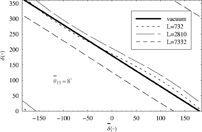
Figure 2: Degenerate value of $\delta$ as a function of true value $\bar{\delta}$, for ${\bar{\theta}}_{13}=8^{\circ}$ and three different baselines; the vacuum result $\delta=\pi-\bar{\delta}$ is also shown.

In vacuum this is not the case. Eq. (8) in the vacuum limit: $C_{-}\rightarrow 0$ or $z\rightarrow\infty$, gives $\delta=\pi-\bar{\delta}$ so that only for ${\bar{\delta}}=\pm\pi/2$ there is no degeneracy. Then the two solutions either break or conserve CP.

In Fig. (2), we show the result of $\delta$ as a function of $\bar{\delta}$ for ${\bar{\theta}}_{13}=8^{\circ}$ for three reference baselines together with the vacuum result. The difference between $\delta$ and ${\bar{\delta}}$ is maximal close to $\bar{\delta}=0^{\circ},180^{\circ}$.

It is interesting to consider the different impact of these degenerate solutions at different baselines. At short baselines, the oscillation probabilities for neutrinos and antineutrinos are approximately the same for two reasons: 1) the relative size of the $\sin\delta$ versus $\cos\delta$ term in eq. (1) is $\tan(\Delta_{13}L/2)\ll 1$, 2) matter effects are irrelevant with the solutions approaching the vacuum case [11, 17]. Indeed, the expansion of eq. (7) for $\Delta_{13}L/2\ll 1$ simplifies to

$$\theta_{13} \simeq \bar{\theta}_{13}-\frac{Y_{+}}{2X_{+}}\left(\cos\delta-\cos\bar{\delta}\right)\,.$$ (12)

The same equation holds for antineutrinos, since $X_{+}(Y_{+})=X_{-}(Y_{-})$ in this approximation. The two equations have collapsed into one, and consequently we expect to find a continuum curve of solutions $(\theta_{13},\delta)$ of the approximate form given by eq. (12). As the baseline increases the probabilities for neutrino and antineutrino oscillations start to differ, not only due to the term in $\sin\delta$, but also because of the matter effects. A shift in $\delta$ cannot in general be then compensated in the neutrino and antineutrino probabilities by a common shift of $\theta_{13}$, and only the two–fold degeneracy discussed above survives.

2.1.2 Solar regime

In this regime the second term in eq. (1) dominates, although the first term cannot be neglected in the analysis of degenerate solutions even for very small values of $\bar{\theta}_{13}$. The reason is that there exist, at fixed neutrino energy and baseline, a pair of values $(\mbox{$\theta_{13}$},\delta)$ at which the first and third terms in eq. (1) exactly compensate both for neutrinos and antineutrinos, in such a way that they are indistinguishable from the situation with ${\bar{\theta}}_{13}=0$ and any $\bar{\delta}$. It is easy to find these values by setting $\bar{\theta}_{13}=0$ in eq. (6) and in the equivalent equation for antineutrinos. $\delta$ is the solution of:

$$\tan\delta=-\frac{1}{z}\,,$$ (13)

and the corresponding $\theta_{13}$ is:

$$\mbox{$\theta_{13}$}=-\frac{Y_{+}}{X_{+}}\cos\left(\delta-\frac{\Delta_{13}L}{2}\right)\,.$$ (14)

Taking as an example $\Delta m^{2}_{23}=3\times 10^{-3}$ eV², $L=2810$ km and $E_{\nu}=0.3E_{\mu},E_{\mu}=50$ GeV, this point is:

$$\mbox{$\theta_{13}$}\sim 1.5^{\circ},\;\;\;\;\;\;\delta\sim-165^{\circ}.$$ (15)

As we will see in the next section, this solution is clearly seen in the fits. Alike to the pattern in the atmospheric regime, this degeneracy occurs only at fixed neutrino energy and baseline.

In summary, this analysis implies that, even with the information from both beam polarities, there are in general two equally probable solutions, at fixed neutrino energy and baseline, for the parameters $\theta_{13}$ and $\delta$. This is of course applicable to any experiment that tries to measure simultaneously $\theta_{13}$ and $\delta$ from the subleading transitions $\nu_{e}\nu_{\mu}$ and ${\bar{\nu}}_{e}{\bar{\nu}}_{\mu}$. These degeneracies can in principle be resolved by exploiting the energy and baseline dependence of the oscillation signals, as will be discussed later on. We point out that a supplementary measurement of the channel $\nu_{e}\nu_{\tau}({\bar{\nu}}_{e}{\bar{\nu}}_{\tau})$ could also be of great help in resolving the degeneracies, if performed with enough accuracy, as the $\delta$-dependent terms in the oscillation probabilities have the opposite sign than for the $\nu_{e}\nu_{\mu}({\bar{\nu}}_{e}{\bar{\nu}}_{\mu})$ transitions. The experimental challenge of measuring those transitions is however much greater and we will not follow this avenue here.

3 Simultaneous determination of $\delta$ and $\theta_{13}$

In [11] a detailed study of the possibility to determine simultaneously $\theta_{13}$ and $\delta$ was performed, but only the range $\theta_{13}>1^{\circ}$ was explored for the LMA-MSW solution. According to Fig. 1, this corresponds to the atmospheric regime. However, the sensitivity to $\theta_{13}$ for the SMA-MSW solution (where only the term $P^{atm}$ survives) was found to extend to smaller values: $\theta_{13}\sim 0.15^{\circ}$ at $\Delta m^{2}_{23}=3\times 10^{-3}$ eV². For the LMA-MSW scenario, such a low value of $\theta_{13}$ lies well inside what we have named the solar regime, which is thus also relevant in the study of CP-violation for $\theta_{13}<1^{\circ}$.

It is very illustrative to consider the different behaviour of the CP asymmetries, defined in [30, 5, 7], in both regimes, as an indication of the sensitivity to CP violation.

The $\delta$-dependent terms in the oscillation probabilities of eq. (1) are linearly suppressed on the two small parameters: $\Delta m^{2}_{12}$ and $\theta_{13}$. In the atmospheric regime the leading term, $P^{atm}$, does not depend on $\Delta m^{2}_{12}$, while it is quadratically dependent on $\theta_{13}$. The sensitivity to CP violation decreases thus linearly with $\Delta m^{2}_{12}$ while it is rather stable as $\theta_{13}$ decreases . There is of course a limit to this CP-insensitivity to $\theta_{13}$ and this is precisely when we enter the solar regime. In the solar regime the role of both parameters is interchanged and while the sensitivity to CP violation decreases linearly with $\theta_{13}$, it remains rather flat with $\Delta m^{2}_{12}$.

This behaviour is shown in Fig. 3, which displays the significance of the CP-odd asymmetries defined in [30, 5, 7] as a function of $\theta_{13}$, for $\Delta m^{2}_{12}$ fixed, and viceversa. In both figures the change in behaviour coincides roughly with the limit between the atmospheric and solar regimes. These asymmetries have been obtained for a muon beam of $50\,{\rm GeV}$ providing $10^{21}$ useful $\mu^{+}$ and $\mu^{-}$ decays and a 40 Kton magnetized iron detector [31], which is our working setup in the present work, as it was in [11].

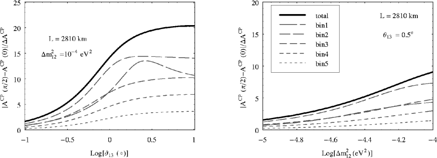
Figure 3: Significance of the asymmetries at $L=2810$ km as a function of $\theta_{13}$ for $E_{\mu}=50$ GeV, $\Delta m^{2}_{12}=10^{-4}$ eV² (left figure) and $\Delta m^{2}_{12}$ for $\theta_{13}=0.5^{\circ}$ (right figure). $\Delta m_{23}^{2}=3\times 10^{-3}$ eV² and $\theta_{12}=\theta_{23}=45^{\circ}$. The five dashed curves correspond to neutrino energy bins of 10 GeV, and the solid curve is the average.

In [11] (see also [13]) $\delta$ and $\theta_{13}$ were extracted from a spectral fit of wrong–sign muons signals for both polarities, using the exact oscillation probabilities in the approximation of constant Earth matter density. Note that an analysis based on CP asymmetries alone does not use all the available information. The observables used were the number of wrong–sign muons in five bins of energy for both beam polarities:

$$N^{\lambda}_{i,\pm},$$ (16)

where $\lambda$ labels the baseline, i the energy bin and $\pm$ the sign of the decaying muons. These numbers are given by:

$$N^{\lambda}_{i,\pm}=\int^{E_{i}+\Delta E}_{E_{i}}\;\Phi_{\nu(\bar{\nu})}(E_{\nu},L)\;\sigma_{\nu(\bar{\nu})}(E_{\nu})\;P_{\nu(\bar{\nu})}(E_{\nu},L,\theta_{13},\delta,{\alpha})$$ (17)

where ${\alpha}$ is the set of remaining oscillation parameters: $\theta_{23},\theta_{12},\Delta m^{2}_{23},\Delta m^{2}_{12}$ and the matter parameter $A$, which were taken as known. $\Phi_{\nu(\bar{\nu})}$ denote the neutrino fluxes and $\sigma_{\nu(\bar{\nu})}$ the DIS cross sections.

Simultaneous $\chi^{2}$ fits of the parameters $\delta$ and $\theta_{13}$ were performed for three reference baselines $L=732$ km (the Cern to Gran Sasso distance or Fermilab to Soudan), $3500$ km (to be replaced in this work by $2810$ km, the distance from Cern to La Palma) and $7332$ km, as well as for various combinations of them.

The $\chi^{2}$ at a fixed baseline is of the generic form:

$$\chi_{\lambda}^{2}=\sum_{i,j}\sum_{p,p^{\prime}}\;(n^{\lambda}_{i,p}-N^{\lambda}_{i,p})C_{i,p:,j,p^{\prime}}^{-1}(n^{\lambda}_{j,p^{\prime}}-N^{\lambda}_{j,p^{\prime}})\,,$$ (18)

where $C$ is the $2N_{bin}\times 2N_{bin}$ covariance matrix. $n^{\lambda}_{i,p}$ are the simulated “data” obtained from a Gaussian or Poisson smearing including backgrounds and efficiencies (for more details we refer to [11]). In the combination of two baselines we have:

$$\chi_{\lambda\lambda^{\prime}}^{2}=\sum_{l,l^{\prime}}\sum_{i,j}\sum_{p,p^{\prime}}\;(n^{l}_{i,p}-N^{l}_{i,p})C_{l,i,p:l^{\prime},j,p^{\prime}}^{-1}(n^{l^{\prime}}_{j,p^{\prime}}-N^{l^{\prime}}_{j,p^{\prime}})\,,$$ (19)

where $C$ is now a matrix of dimension $4N_{bin}\times 4N_{bin}$

As the errors on the ${\alpha}$ were neglected, $C$ contained only statistical errors, $\delta n^{l}_{i,p}$, which were assumed to be independent for different $i$, $p$ and $l$:

$$C_{l,i,p;l^{\prime},j,p^{\prime}}\equiv\delta_{ll^{\prime}}\;\delta_{ij}\;\delta_{pp^{\prime}}\;({\delta n}^{l}_{i,p})^{2}.$$ (20)

In [11] only the restricted range $0<\delta<90^{\circ}$ and $\theta_{13}>1^{\circ}$ was explored. For this reason the degeneracies appearing when the full range of $\delta$ is considered were missed. We have repeated the analysis by considering the full range of $\delta$ and $\theta_{13}$. In all the plots that follow realistic efficiencies and backgrounds have been included. We have checked that the degenerate images in the plots shown below appear at the points indicated by the analysis of the previous section. The false images are somewhat softened, as different neutrino and antineutrino energies enter in the analysis, but still visible. We present fits only for $\Delta m^{2}_{23}>0$. The opposite case gives better results: for $\Delta m^{2}_{23}<0$, the statistics for the signals of positive and negative wrong–sign muons are closer (so that the difference is more neatly seen) because matter effects enhance in this case $P_{{\bar{\nu}}_{e}{\bar{\nu}}_{\mu}}$, compensating to a large extent the difference in the neutrino DIS cross sections $\sigma_{\nu}\simeq 2\sigma_{\bar{\nu}}$.

All the results shown below correspond to central values of the parameters in the LMA-MSW scenario: $\Delta m^{2}_{12}=10^{-4}$ eV², $\Delta m_{23}^{2}=3\times 10^{-3}$ eV² and $\theta_{12}=\theta_{23}=45^{\circ}$, except in Fig. 12, where the full range of $\Delta m^{2}_{12}$ is considered.

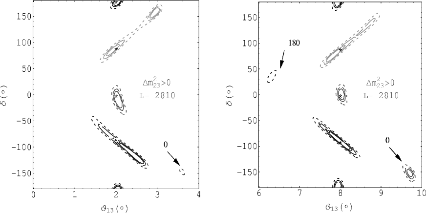
Figure 4: Simultaneous fits of $\delta$ and $\theta_{13}$ at $L=2810$ km for different central values (indicated by the stars) of $\bar{\delta}=-90^{\circ},0^{\circ},90^{\circ},180^{\circ}$ and ${\bar{\theta}}_{13}=2^{\circ}$ (left), $8^{\circ}$ (right). The value of $\bar{\delta}$ for the degenerate solutions is also indicated.

3.1 Atmospheric regime

Recall that the pure CP-effects peak at distances in the range $2000$–$4000$ km [5, 7, 11]. In Figs. 4 we show the results of the fits including efficiencies and backgrounds for $L=2810$ km for central values of ${\bar{\delta}}=-90^{\circ},0^{\circ},90^{\circ},180^{\circ}$ and for $\bar{\theta}_{13}=2^{\circ}$ (left) and $\bar{\theta}_{13}=8^{\circ}$ (right). The energy dependence of the signals is not significant enough (with our setup) to resolve the expected two-fold degeneracy. The second solution is clearly seen for the central value of ${\bar{\delta}}=0^{\circ}$ as an isolated island. For the central values ${\bar{\delta}}=-90^{\circ}$ and ${\bar{\delta}}=90^{\circ}$, the degeneracy is responsible for the rather large contours which encompass the two solutions. Notice that as ${\bar{\theta}}_{13}$ diminishes the fake solution for $\bar{\delta}=90^{\circ}$ moves towards $\delta=180^{\circ}$, as it should (recall that, in the solar regime, the vacuum fake image lies at $\delta=180^{\circ}$).

Figs. 5 show the fits for ${\bar{\theta}}_{13}=8^{\circ}$ at $L=732$ km and $7332$ km. In the former, the expected continous line of solutions of the form given by eq. (12) is clearly seen. The measurement of $\delta$ is thus impossible at this baseline if $\theta_{13}$ is unknown. In the longer baseline, the sensitivity to $\delta$ is similarly lost but for a different reason: the CP-signal is fading away (indeed the underlying degenerate solutions become much closer in $\theta_{13}$) and statistics is diminishing.

In Fig. 6 we show the result of combining any two baselines. The two-fold degeneracy does not disappear completely in the combination of the two shorter baselines, while it does in the remaining two combinations. It is interesting that, while the shorter and longer baselines by themselves are not appropiate for CP studies, their combination is quite promising, due to the very different pattern shown by the correlation between $\theta_{13}$ and $\delta$ in each of them. The overall conclusion is that the combination of any two distances is interesting regarding CP violation.

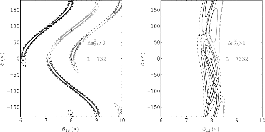
Figure 5: Simultaneous fits of $\delta$ and $\theta_{13}$ at $L=732$ km (left) and $L=7332$ km (right) for different central values of $\bar{\delta}=-90^{\circ},0^{\circ},90^{\circ},180^{\circ}$ and $\bar{\theta}_{13}=8^{\circ}$.

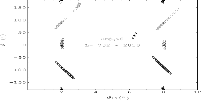
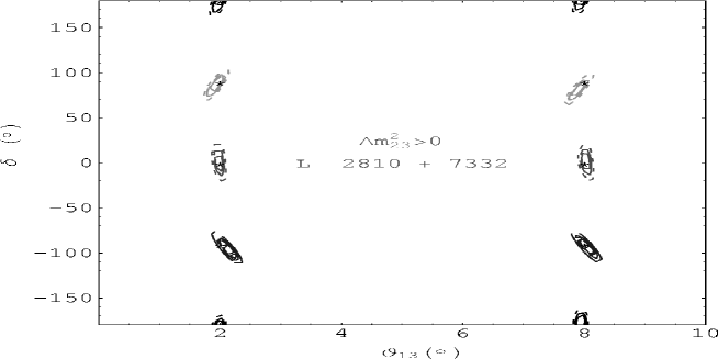
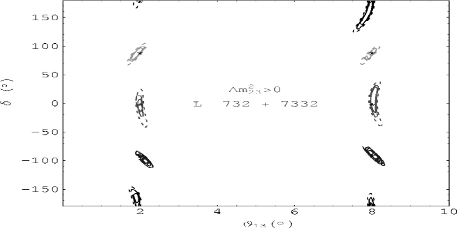
Figure 6: Fits of $\delta$ and $\theta_{13}$ combining any two baselines.

3.2 Solar regime

In Fig. 7 we show the results of the fits including efficiencies and backgrounds for $L=2810$ km for central values of ${\bar{\delta}}=-90^{\circ},0^{\circ},90^{\circ},180^{\circ}$ and for ${\bar{\theta}}_{13}=0.3^{\circ}$ (left) and ${\bar{\theta}}_{13}=0.6^{\circ}$ (right). Consider for instance the case ${\bar{\theta}}_{13}=0.3^{\circ}$ (left): the degenerate images of the four points chosen appear grouped at the right/lower side of the figure. These are the solutions that mimic $\theta_{13}=0$ as predicted in section 2.1.2. The position of these solutions can be accurately predicted from the analysis of the previous section. The comparison of these figures with Fig. 4 illustrates the expected decrease of the sensitivity to CP violation for very small $\theta_{13}$, consistent with the behaviour of the significance of the CP-asymmetry in the solar regime shown in Fig. 3. Note that at ${\bar{\theta}}_{13}=0.3$, the sensitivity to CP is already lost for ${\bar{\delta}}=-90^{\circ}$.

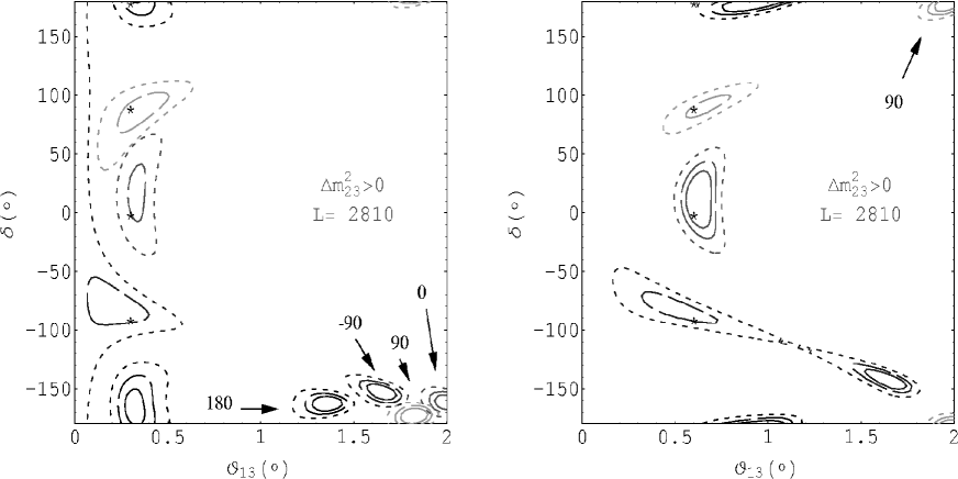
Figure 7: Simultaneous fits of $\delta$ and $\theta_{13}$ at $L=2810$ km, for different central values of $\bar{\delta}=-90^{\circ},0^{\circ},90^{\circ},180^{\circ}$ and ${\bar{\theta}}_{13}=0.3^{\circ}$ (left), $0.6^{\circ}$ (right). The value of $\bar{\delta}$ for the degenerate solutions is indicated.

In Fig. 8 we show the result of combining the baselines $L=2810$ km and $L=732$ km with the longer one. As in the atmospheric regime, the degeneracies are nicely resolved in the combination of the intermediate and long baselines. However, in this case the combination of the short and long baselines is not as good. Note the degenerate solution that survives for $\bar{\delta}=90^{\circ}$ which appears centered at $\delta=-90^{\circ}$. This is the result of the intersection of the approximately vertical contours found at $L=7332$ km with the $\cos\delta$ contours at $L=732$ km (see Fig. 5).

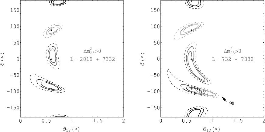
Figure 8: Simultaneous fits of $\delta$ and $\theta_{13}$ at two combinations of baselines, $L=2810+7332$ km (left) and $L=732+7332$ km (right), for ${\bar{\theta}}_{13}=0.6^{\circ}$ and different central values of $\bar{\delta}=-90^{\circ},0^{\circ},90^{\circ},180^{\circ}$.

4 New analysis: inclusion of expected errors on oscillation parameters and matter density

Consider the uncertainty in the theoretical parameters ${\alpha}$. These errors induce in general a correlation between the observables, $N^{\lambda}_{i,\pm}$, which has to be taken into account. The matrix $C$ of eq. (19) is of the form:

$$C_{l,i,p;l^{\prime},j,p^{\prime}}\equiv\delta_{ll^{\prime}}\;\delta_{ij}\;\delta_{pp^{\prime}}\;({\delta n}^{l}_{i,p})^{2}+\sum_{\alpha}\;\frac{\partial N^{l}_{i,p}}{\partial\alpha}\frac{\partial N^{l^{\prime}}_{j,p^{\prime}}}{\partial\alpha}\;\sigma^{2}(\alpha),$$ (21)

where $\sigma(\alpha)$ is the 1$\sigma$ error on the parameter $\alpha$.

Recent analysis of the expected uncertainty in the knowledge of the atmospheric parameters at the neutrino factory indicate a $\sim 1\%$ uncertainty in $\Delta m_{23}^{2}$ and $\sin^{2}2\theta_{23}$ [25, 26] For the solar parameters we include the results of the analyses of the Kamland reach [27]: $2\%$ error in $\Delta m_{12}^{2}$ and $\pm 0.04$ in $\sin^{2}2\theta_{12}$, for maximal $\theta_{12}$, both at $1\sigma$. Slightly smaller errors could be obtained for the product $(\sin 2\theta_{12}\,\Delta m^{2}_{12})^{2}$ which is the combination entering the relevant oscillation probabilities [32], a refinement we neglect here. For the uncertainty on the matter parameter, $A$, we could not find any estimate in the literature. The dispersion of the different models of the Earth density profile [33] indicates an uncertainty of $1$–$2\%$ for trajectories which do not cross the core, though. We consider a range between $1$–$10\%$ for illustration.

The most important changes result from the uncertainty in $\theta_{23}$ and in the matter parameter $A$, with the former affecting mainly the measurement of $\theta_{13}$ and the latter the sensitivity to $\delta$.

Recall Fig. 4, where no errors on the oscillation and matter parameters were included. Fig. 9 (left) depicts the results for ${\bar{\delta}}=90^{\circ}$ and $-90^{\circ}$ at $L=2810$ km, including all errors (with an error in the matter parameter of $1\%$) compared (right) with the situation in which only the error on the atmospheric angle $\theta_{23}$ is included. The two graphics in this figure are almost identical, showing that the dominant error is that of $\theta_{23}$. It affects mainly the determination of $\theta_{13}$, a fact easy to understand: while the measurement of the leading transition $\nu_{\mu}\rightarrow\nu_{\tau}$ is sensitive to $\sin^{2}2\theta_{23}$, and this can be measured with a $1\%$ uncertainty, the subleading transition $\nu_{e}\rightarrow\nu_{\mu}$ is proportional to $\sin^{2}\theta_{23}$. For maximal $\theta_{23}$ mixing a $1\%$ relative error in the former translates into a $6\%$ in the latter. This is then the largest relative error of all the parameters that enter $P^{atm}$, which is dominant in most of the parameter space. Note that the effect of the errors is more important for larger $\bar{\theta}_{13}$. In Fig. 10 we show the results for the best combination of baselines when all errors have been included. The resolution of the degeneracies discussed in the previous sections is still achieved, but the contours have become sizeably larger.

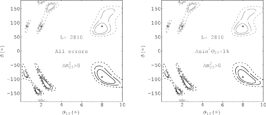
Figure 9: Fits of $\delta$ and $\theta_{13}$ for various central values of ${\bar{\delta}}$ and ${\bar{\theta}}_{13}$ at $L=2810$ km including all the errors on the remaining parameters (left plot) with $\Delta A/A=1\%$ and including only the error on $\theta_{23}$ (right plot).

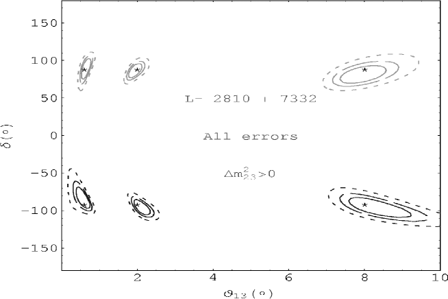
Figure 10: Fits of $\delta$ and $\theta_{13}$ combining the two baselines: $2810$ km and $7332$ km, for various central values of ${\bar{\delta}}$ and ${\bar{\theta}}_{13}$ including all the errors on the remaining parameters with $\Delta A/A=1\%$.

The uncertainty in $A$ is more relevant for the determination of $\delta$, although if this error is controlled at the percent level the effect is negligible. In general, even for $\Delta A/A=10\%$, the effect is far less important than the error induced by correlations between $\theta_{13}$ and $\delta$. This can be seen with just one baseline, where the degeneracies survive. As an illustration, in Fig. 11 for L=$2810$ km, $\Delta A/A$ is varied in the range $1-10\%$, with $\bar{\delta}=90^{\circ}$, $\bar{\theta}_{13}=8^{\circ}$ and the errors on the remaining oscillation parameters included. This is to be compared with Fig. 4 (right) where no uncertainties were assumed. The error in $\delta$ is seen to be mostly dominated by the correlation of $\theta_{13}$ and $\delta$. For the combination $L=2810+7332$ km, where the degeneracies are resolved, the effect of the error in A is more important in relative terms (compare Fig. 10 with the middle plot in Fig. 6): a $10\%$ error in $A$ is a $50\%$ increase of the error in $\delta$.

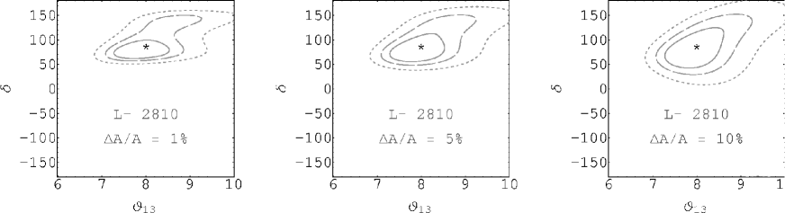
Figure 11: Results from a simultaneous fits to $\theta_{13},\delta$ for ${\bar{\delta}}=90^{\circ}$ including errors on the oscillation parameters and varying the error on the average Earth matter density from $1\%=10\%$.

It is clearly desirable to have a per cent control over the average Earth matter density, which does not look a priori unrealistic.

Recently, the authors of [20] have presented an analysis of the sensitivity to CP violation, including the errors on the oscillation and matter parameters, with quite different conclusions. In particular, they state that CP violation can only be measured in a small window at the shorter baselines. There are a number of differences between their analysis and ours. They do not consider the simultaneous determination of $\theta_{13}$ and $\delta$, but include and ad hoc $10\%$ error on $\theta_{13}$. They assume as well larger errors on the remaining solar and atmospheric parameters: a democratic $10\%$. We have seen that estimates from Kamland and the expectation from disappearance measurements at the neutrino factory give more optimistic results. Finally, they do not take into account correlations of the errors that these parameters induce on the different observables: wrong–sign muons in different energy bins and different polarities. Neither they include experimental background and efficiencies.

Let us turn now to the case of smaller values of $\Delta m^{2}_{12}$ allowed in the LMA-MSW range. For fixed $\theta_{13}$, the sensitivity to $\delta$ decreases linearly with $\Delta m^{2}_{12}$ in the atmospheric regime and more slowly in the solar one. For the plots in the atmospheric regime of this section it does not necessarily imply, though, a linear scaling (with $\Delta m^{2}_{12}$) of the error in $\delta$, as the latter is mostly dominated by the existence of degenerate solutions on the plane ($\theta_{13},\delta$), whose separation dos not follow such a linear pattern.

It is interesting to understand how much of the LMA-MSW range can be covered in the discovery of CP violation. This is illustrated in Fig. 12 with a rough exclusion plot. For the hypothetical nature values ${\bar{\delta}}=90^{\circ}$ and the best combination of baselines, $L=2810+7332$ km, the line corresponds to the minimum value of $\Delta m^{2}_{12}$ at which the $99\%$CL error on the phase reaches $90^{\circ}$ degrees, and is thus indistinguishable from $0^{\circ}$ or $180^{\circ}$ (i.e. no CP violation). The error on the phase is computed by taking the longest vertical size (upwards or downwards, whichever is longest) of the $99\%$CL contour from $90^{\circ}$. All errors on the parameters have been included. With this definition, there is sensitivity to CP violation for $\mbox{$\theta_{13}$}>$ few tenths of degree and $\Delta m^{2}_{12}>3\times 10^{-4}$ eV².

An analogous plot in [11] indicated better sensitivity. Several reasons account for the difference. First, only the possibility of separating $90^{\circ}$ from $0^{\circ}$ (instead of $180^{\circ}$, which is more constraining [20]) was considered there. Second, the correlation between $\theta_{13}$ and $\delta$ was not taken into account: in order words, $\theta_{13}$ was fixed at its true value ${\bar{\theta}}_{13}$ and only then the error on $\delta$ considered. Finally, the errors on the remaining oscillation parameters and $A$ were not included, although this makes a very small difference if $\Delta A/A=1\%$.

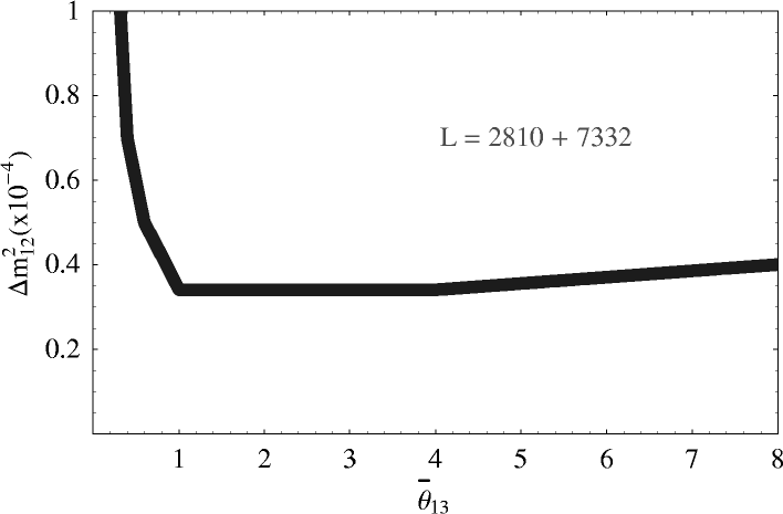
Figure 12: Sensitivity reach for CP violation as defined in the text on the plane $(\Delta m^{2}_{12},{\bar{\theta}}_{13})$ for the combination of baselines L = 2810 and 7332 km. All errors are included.

A final comment. As stated before, the problem of the correlations between $\theta_{13}$ and $\delta$ has to be faced by any experiment measuring just the $\nu_{e}\leftrightarrow\nu_{\mu}$ and $\bar{\nu}_{e}\leftrightarrow\bar{\nu}_{\mu}$ transitions. In particular this applies to the so-called “superbeams” [34]: intense neutrino beams from pion (and kaon) decay. They could provide, though, very useful complementary information to the neutrino factory in disentangling $\theta_{13}$ and $\delta$, for their expected reach $\theta_{13}>3^{\circ}$[34].

5 Conclusions

A neutrino factory from muon storage rings, with muon energies of a few dozen GeV, is an appropiate facility to discover leptonic CP violation through wrong–sign muon searches. This requires that the solution to the neutrino solar deficit is confirmed to lie in the LMA-MSW regime, and the angle $\theta_{13}$ is larger than a few tenths of degree. Within this range, the sensitivity to CP-violation is lost only for the smaller values of the solar mass difference allowed by the LMA-MSW scenario.

At the hypothetical time of the neutrino factory, the value of the parameters $\theta_{13}$ and $\delta$ may be still unknown and will have to be simultaneously measured. In this paper we have considered the full range of possible values of $\delta$. A relevant problem unearthed is the generic existence, at a given (anti)neutrino energy and fixed baseline, of a second value of the set ($\mbox{$\theta_{13}$},\delta$) which gives the same oscillation probabilities for neutrinos and antineutrinos than the true value chosen by nature. It is a generic challenge for any future facility. The spectral analysis and the combination of baselines satisfactorily resolves this degeneracy.

Furthermore, we have included in the analysis the expected uncertainty on the knowledge of the rest of the oscillation parameters ($\sin^{2}\theta_{23},\,\Delta m^{2}_{23},\,\sin^{2}\theta_{12},\,\Delta m^{2}_{12}$) and on the Earth electron density. Noticeable changes result from the error on $\theta_{23}$, which affects mainly the uncertainty in $\theta_{13}$, and from the uncertainty on the Earth matter profile, which affects mainly the extraction of $\delta$. The latter uncertainty is of little consequence if at the level of a few percent. It seems pertinent to us that a detailed geological analysis of the planned baselines is performed, to reinforce the expectations as regards CP violation.

Realistic background detection errors and experimental efficiencies have been included in the analysis. The overall conclusion is that the optimal distance for studying CP-violation effects with neutrino energies of few dozens of GeV is still of $O(3000)$ km, although the combination of two baselines, one of which being preferably a very long one, is very important in resolving degeneracies.

6 Acknowledgements

We thank J. Bahcall, A. Cervera, A. Donini, A. de Gouvea, P. Lipari, H. Murayama, A. Pierce and S. Rigolin for useful conversations and exchanges. We are specially indebted to A. Cervera, A. Donini and S. Rigolin for earlier collaboration on this subject and their contribution to the early stages of this work. We acknowledge as well discussions with J. Sato. This work has been partially supported by CICYT projects AEN/97/1678, AEN/99/0692 and GCPA640 as well as the Generalitat Valenciana project GV99-3-1-01.

References

- [1] L. Wolfenstein, Phys. Rev. D17 (1978) 2369; D20 (1979) 2634; S.P. Mikheyev and A. Smirnov, Sov. J. Nucl. Phys. 42 (1986) 913.
- [2] For a recent global analysis of solar data and atmospheric data see for instance M.C. González-García et al, Phys. Rev. D63 (2001) 033005.
- [3] B. Pontecorvo, Sov. Phys. JETP 26 (1968) 984.
- [4] J. Arafune, M. Koike and J. Sato, Phys. Rev. D56 (1997) 3093. Phys. Lett. B345 (1998) 373. H. Minakata and H. Nunokawa, Phys. Lett. B413 (1997) 369; Phys. Rev. D57 (1998) 4403. S.M. Bilenky, C. Giunti and W. Grimus, Phys.Rev. D58 (1998) 033001. M. Tanimoto, Phys. Lett. B462 (1999) 115.
- [5] A. de Rújula, M. B. Gavela and P. Hernández, Nucl. Phys. B547 (1999) 21.
- [6] K. Dick et al, Nucl. Phys. B562 (1999) 299.
- [7] A. Donini et al, Nucl.Phys. B574 (2000) 23.
- [8] A. Romanino, Nucl. Phys. B574 (2000) 675.
- [9] G. Barenboim and F. Scheck, Phys.Lett. B475 (2000) 95.
- [10] M. Freund et al, Nucl. Phys. B578 (2000) 27.
- [11] A. Cervera et al., Nucl. Phys. B579 (2000) 17; Erratum-ibid. B593 (2001) 731.
- [12] J. Bernabeu and M.C. Banuls, Nucl. Phys. Proc. Suppl. 87 (2000) 315.
- [13] A. Bueno, M. Campanelli and A. Rubbia, Nucl. Phys. B589 (2000) 577.
- [14] V. Barger, S. Geer and K. Whisnant, Phys. Rev. D61 (2000) 053004.
- [15] H. Minakata and H. Nunokawa, Phys. Lett. B495(2000)369.
- [16] S.J. Parke and T.J. Weiler, Phys. Lett. B501(2001) 106.
- [17] P. Lipari, hep-ph/0102046.
- [18] D.G. Kosharev, CERN internal report CERN/ISR-DI/74-62 (1974).
- [19] S. Geer, Phys. Rev. D57 (1998); 6989; and erratum.
- [20] M. Koike, R. Ota and J. Sato, hep-ph/0011387 and hep-ph/0103024.
- [21] S.H. Ahn et al., K2K Collaboration, hep-ex/0103001. E. Ables et al.,MINOS Collaboration, FERMILAB-PROPOSAL-P-875, Feb 1995; FERMILAB-PROPOSAL-P-875-ADD, NUMI-L-79, Apr 1995. M. Guler et al., OPERA Collaboration, CERN-SPSC-2000-028, CERN-SPSC-P-318, LNGS-P25-00, Jul 2000.
- [22] The KamLAND proposal, Stanford-HEP-98-03; http://kamland.lbl.gov/KamLAND.US.Proposal.pdf.
- [23] D. A. Petyt, Thesis submitted to Univ. of Oxford, England, 1998.
- [24] Super Kamiokande collaboration, Phys. Rev. Lett. 81 (1998) 1562. L. Fogli et al., Nucl. Instrum. Meth. A451 (2000) 10.
- [25] V. Barger et. al., Phys. Rev. D62 (2000) 013004.
- [26] M.C. González-García, talk at the CERN Nufact neutrino oscillation working group, February 2000.
- [27] V. Barger, D. Marfatia and B.P. Wood, hep-ph/0011251. H. Murayama and A. Pierce, hep-ph/0012075.
- [28] H. W. Zaglauer and K. H. Schwarzer, Z. Phys. C 40 (1988) 273.
- [29] R. Gandhi et. al., Astropart. Phys. 5 (1996) 81.
- [30] N. Cabibbo, Phys. Lett. B72 (1978) 33.
- [31] A. Cervera, F. Dydak and J.J. Gómez-Cadenas, Nucl. Instrum. Meth. A451 (2000) 123.
- [32] A. Pierce, private communication.
- [33] J.N. Bahcall and P.I. Krastev, Phys. Rev. C56 (1997) 2839. J.N. Bahcall, private comunication.
- [34] B. Richter, hep-ph/0008222. K. Dick et al, hep-ph/0008016. V. Barger et al, hep-ph/0012017. A. Blondel, M. Dóndega and S. Gilardoni, CERN NuFact Note 2000-53. M. Mezzetto, CERN NuFact Note 2000-60. Talk by J.J. Gómez-Cadenas at Venice Workshop on Neutrino Telescopes http://axpd24.pd.infn.it/conference2001/venice01.html.