1 Introduction

The study of $\pi\pi$ scattering is a classical subject in the field of strong interactions. The properties of the pions are intimately related to an approximate symmetry of QCD. In the chiral limit, where $m_{u}$ and $m_{d}$ vanish, this symmetry becomes exact, the Lagrangian being invariant under the group SU(2)${}_{\mbox{\tiny R}}\times$SU(2)${}_{\mbox{\tiny L}}$ of chiral rotations. The symmetry is spontaneously broken to the isospin subgroup SU(2)${}_{\mbox{\tiny V}}$. The pions represent the corresponding Goldstone bosons.

In reality, the quarks are not massless. The theory only possesses an approximate chiral symmetry, because $m_{u}$ and $m_{d}$ happen to be very small. The consequences of the fact that the symmetry breaking is small may be worked out by means of an effective field theory [1]. The various quantities of interest are expanded in powers of the momenta and quark masses. In the case of the pion mass, for instance, the expansion starts with [2]

$$M_{\pi^{+}}^{2}=(m_{u}+m_{d})\,B+O(m^{2})\,,\hskip 20.00003ptB=\frac{1}{F^{2}}\,|\langle 0|\,\overline{\rule[4.19998pt]{3.99994pt}{0.0pt}}uu\,|0\rangle|\,,$$ (1.1)

where $F$ is the value of the pion decay constant in the chiral limit, $m_{u},m_{d}\rightarrow 0$. The formula shows that the square of the pion mass is proportional to the product of $m_{u}+m_{d}$ with the order parameter $\langle 0|\,\overline{\rule[4.19998pt]{3.99994pt}{0.0pt}}uu\,|0\rangle$. The two factors represent quantitative measures for explicit and spontaneous symmetry breaking, respectively. If the explicit symmetry breaking is turned off, the pions do become massless, as they should: The symmetry is then exact, so that the spectrum contains three massless Goldstone bosons, while all other levels form massive, degenerate isospin multiplets.

The properties of the Goldstone bosons are strongly constrained by chiral symmetry: In the chiral limit, the scattering amplitude vanishes when the momenta of the pions tend to zero. To first order in the symmetry breaking, the $S$–wave scattering lengths are proportional to the square of the pion mass [3]:

$$a_{0}^{0}=\frac{7M_{\pi}^{2}}{32\,\pi F_{\pi}^{2}}\,,\hskip 20.00003pta_{0}^{2}=-\frac{M_{\pi}^{2}}{16\,\pi F_{\pi}^{2}}\,,$$ (1.2)

where $a_{\ell}^{I}$ stands for the scattering length in the isospin $I$ channel with angular momentum $\ell$. The two low energy theorems (1.2) are valid only at leading order in a series expansion in powers of the quark masses: The next–to–leading order corrections were calculated in [4], and even the next–to–next–to–leading order corrections are now known [5].

In the following, we exploit the fact that analyticity, unitarity and crossing symmetry impose further constraints on the scattering amplitude. These were analyzed in detail in [6], on the basis of the Roy equations [7] and of the experimental data available at intermediate energies. The upshot of that analysis is that $a_{0}^{0}$ and $a_{0}^{2}$ are the essential low energy parameters: Once these are known, the available experimental data determine the low energy behaviour of the $\pi\pi$ scattering amplitude to within remarkably small uncertainties. As discussed above, chiral symmetry predicts exactly these two parameters. Hence the low energy behaviour of the scattering amplitude is fully determined by the experimental data in the intermediate energy region and the theoretical properties just mentioned: analyticity, unitarity, crossing symmetry and chiral symmetry.

The resulting predictions for the $S$–wave scattering lengths were presented already [8]. The purpose of the present paper is to (i) discuss the analysis that underlies these predictions in more detail, (ii) present the results for the threshold parameters of the $P$–, $D$–, and $F$–waves, (iii) give an explicit representation for the $S$– and $P$–wave phase shifts and (iv) extract the information about the coupling constants of the effective Lagrangian.

Several authors have performed a comparison of the chiral perturbation theory predictions with the data, in particular also in view of a determination of the effective coupling constants $\ell_{1}$ and $\ell_{2}$ [9]–[22]. Stern and collaborators [23, 24] investigate the problem from a different point of view, referred to as “Generalized Chiral Perturbation Theory”. These authors treat the $S$–wave scattering lengths as free parameters and investigate the possibility that their values strongly deviate from those predicted by Weinberg. In the language of the effective chiral Lagrangian, this scenario would arise if the standard estimates for the effective coupling constant $\ell_{3}$ were entirely wrong: The quark condensate would then fail to represent the leading order parameter of the spontaneously broken chiral symmetry. Indeed, these estimates rely on a theoretical picture that has not been tested experimentally.

On the experimental side, the situation is the following. As shown in early numerical analyses of the Roy equations [25], only data sufficiently close to threshold can provide significant bounds on the scattering lengths. The often quoted values $a_{0}^{0}=0.26\pm 0.05$, $a_{0}^{2}=-0.028\pm 0.012$ [26, 27] mainly rely on the $3\cdot 10^{4}$ $K\rightarrow\pi\pi e\nu$ decays collected by the Geneva-Saclay collaboration, which provided its final results in 1977 [28]. There are new data from Brookhaven [29, 30], where more than $4\cdot 10^{5}$ $K_{e_{4}}$ decays are being analyzed, and the low energy behaviour of the relevant form factors is now also known much better [32, 22]. As will be discussed in section 13, the preliminary results of this experiment indeed reduce the uncertainties significantly. A similar experiment is proposed by the NA48 collaboration at CERN [33]. Unfortunately, the data taking at the DA$\Phi$NE facility is delayed, due to technical problems with the accelerator. A beautiful experiment is under way at CERN [34], which is based on the fact that $\pi^{+}\pi^{-}$ atoms decay into a pair of neutral pions, through the strong transition $\pi^{+}\pi^{-}\!\rightarrow\!\pi^{0}\pi^{0}$. Since the momentum transfer nearly vanishes, only the scattering lengths are relevant: At leading order in isospin breaking, the transition amplitude is proportional to $a_{0}^{0}\!-\!a_{0}^{2}$. The corrections at next–to–leading order are now also known [35], as a result of which a measurement of the lifetime of a $\pi^{+}\pi^{-}$ atom amounts to a measurement of this combination of scattering lengths. Finally, we mention the new data on pion production off nucleons, obtained by the CHAOS collaboration at Triumf [36]. The scattering lengths may be extracted from these data by means of a Chew-Low extrapolation procedure. Chiral symmetry, however, suppresses the one-pion exchange contribution with a factor of $t$, so that a careful data selection is required to arrive at a coherent Chew-Low fit. It yet remains to be seen whether these data permit a significant reduction of the uncertainties in the experimental determination of $a_{0}^{0}$ and $a_{0}^{2}$.

The experiments mentioned above are of particular interest, because they offer a test of the hypothesis that the quark condensate represents the leading order parameter of the spontaneously broken symmetry: If the predictions obtained in the present paper should turn out to be in contradiction with the outcome of these experiments, the commonly accepted theoretical picture would require thorough revision.

2 Chiral representation

Throughout the present paper we work in the isospin limit: We disregard the e.m. interaction and set $m_{u}=m_{d}=m$. The various elastic reactions among two pions may then be represented by a single scattering amplitude $A(s,t,u)$. Only two of the Mandelstam variables are independent, $s+t+u=4M_{\pi}^{2}$ and, as a consequence of Bose statistics, the amplitude is invariant under an interchange of $t$ and $u$.

As discussed in detail in ref. [9], chiral perturbation theory allows one to study the properties of the $\pi\pi$ scattering amplitude that follow from the occurrence of a spontaneously broken approximate symmetry. The method is based on a systematic expansion in powers of the momenta and of the light quark masses. We refer to this as the chiral expansion and use the standard bookkeeping, which counts the quark masses like two powers of momentum, $m=O(p^{2})$.

The two loop representation of the scattering amplitude given in [5] yields the first three terms in the chiral expansion of the partial waves:

$$t^{I}_{\ell}(s)=t^{I}_{\ell}(s)_{2}+t^{I}_{\ell}(s)_{4}+t^{I}_{\ell}(s)_{6}+O(p^{8})$$ (2.1)

At leading order, only the $S$– and $P$–waves are different from zero:

$$t^{0}_{0}(s)_{2}=\frac{2s-M_{\pi}^{2}}{32\pi F_{\pi}^{2}}\,,\hskip 20.00003ptt^{1}_{1}(s)_{2}=\frac{s-4M_{\pi}^{2}}{96\pi F_{\pi}^{2}}\,,\hskip 20.00003ptt^{2}_{0}(s)_{2}=-\frac{s-2M_{\pi}^{2}}{32\pi F_{\pi}^{2}}\,.$$ (2.2)

In the low energy expansion, inelastic reactions start showing up only at $O(p^{8})$. The unitarity condition therefore reads:

$$\mbox{Im}\,t^{I}_{\ell}(s)=\sigma(s)\,|\hskip 0.39993ptt^{I}_{\ell}(s)\hskip 0.29999pt|^{2}+O(p^{8})\,,\hskip 20.00003pt\sigma(s)=\sqrt{1-\frac{4M_{\pi}^{2}}{s}}\,.$$ (2.3)

The condition immediately implies that the imaginary parts of the two loop amplitude may be worked out from the one-loop representation:

$$\mbox{Im}\,t_{\ell}^{I}(s)=\sigma(s)\,t_{\ell}^{I}(s)_{2}\,\left\{t_{\ell}^{I}(s)_{2}+2\,\mbox{Re}\,t_{\ell}^{I}(s)_{4}\right\}+O(p^{8})$$ (2.4)

The formula shows that, at low energies, the imaginary parts of the partial waves with $\ell\geq 2$ are of order $p^{8}$ and hence beyond the accuracy of the two loop calculation.

Stated differently, the imaginary part of the two loop representation is due exclusively to the $S$– and $P$–waves. This implies that, up to and including $O(p^{6})$, the chiral representation of the scattering amplitude only involves three functions of a single variable:

$$A(s,t,u) \!\!\!= \!\!\!C(s,t,u)+32\pi\left\{\mbox{$\frac{1}{3}$}\,U^{0}(s)+\mbox{$\frac{3}{2}$}\,(s-u)\,U^{1}(t)+\mbox{$\frac{3}{2}$}\,(s-t)\,U^{1}(u)\right.$$ (2.5)

$$\!\!\!\left.+\mbox{$\frac{1}{2}$}\,U^{2}(t)+\mbox{$\frac{1}{2}$}\,U^{2}(u)-\mbox{$\frac{1}{3}$}\,U^{2}(s)\right\}+O(p^{8})\,.$$

The first term is a crossing symmetric polynomial in $s$, $t$, $u$,

$$C(s,t,u)=c_{1}+s\,c_{2}+s^{2}\,c_{3}+(t-u)^{2}\,c_{4}+s^{3}\,c_{5}+s\,(t-u)^{2}\,c_{6}\,.$$ (2.6)

The functions $U^{0}(s)$, $U^{1}(s)$ and $U^{2}(s)$ describe the “unitarity corrections” associated with $s$–channel isospin $I=0,1,2$, respectively. In view of the fact that the chiral perturbation theory representation for the imaginary parts of the partial waves grows with the power $\mbox{Im}\,t^{I}_{\ell}(s)_{6}\propto s^{3}$, we need to apply several subtractions for the dispersive representation of these functions to converge. It is convenient to subtract at $s=0$ and to write the dispersion integrals in the form

$$U^{0}(s) \!\!\!= \!\!\!\frac{s^{4}}{\pi}\int_{4M_{\pi}^{2}}^{\infty}ds^{\prime}\;\frac{\sigma(s^{\prime})\,t_{0}^{0}(s^{\prime})_{2}\,\{t_{0}^{0}(s^{\prime})_{2}+2\,\mbox{Re}\,t_{0}^{0}(s^{\prime})_{4}\}}{s^{\prime\,4}(s^{\prime}-s)}\,,$$

$$U^{1}(s) \!\!\!= \!\!\!\frac{s^{3}}{\pi}\int_{4M_{\pi}^{2}}^{\infty}ds^{\prime}\;\frac{\sigma(s^{\prime})\,t_{1}^{1}(s^{\prime})_{2}\,\{t_{1}^{1}(s^{\prime})_{2}+2\,\mbox{Re}\,t_{1}^{1}(s^{\prime})_{4}\}}{s^{\prime\,3}(s^{\prime}-4M_{\pi}^{2})\,(s^{\prime}-s)}\,,$$ (2.7)

$$U^{2}(s) \!\!\!= \!\!\!\frac{s^{4}}{\pi}\int_{4M_{\pi}^{2}}^{\infty}ds^{\prime}\;\frac{\sigma(s^{\prime})\,t_{0}^{2}(s^{\prime})_{2}\,\{t_{0}^{2}(s^{\prime})_{2}+2\,\mbox{Re}\,t_{0}^{2}(s^{\prime})_{4}\}}{s^{\prime\,4}(s^{\prime}-s)}\,.$$

The subtraction constants are collected in the polynomial $C(s,t,u)$. Alternatively, we could set $C(s,t,u)=0$ and book the subtraction terms as polynomial contributions to $U^{0}(s)$, $U^{1}(s)$, $U^{2}(s)$. The decomposition of $C(s,t,u)$ into a set of three polynomials of a single variable is not unique, however, so that we would have to adopt a convention for this splitting – we find it more convenient to work with the above representation of the amplitude.

The specific structure of the unitarity correction given above was noted already in [23]. It is straightforward to check that the explicit result of the full two loop calculation described in [5] is indeed of this structure. The essential result of that calculation is the expression for the polynomial part of the amplitude, in terms of the effective coupling constants. The corresponding formulae, which specify how the coefficients $c_{1},\ldots,\,c_{6}$ depend on the quark masses, are given in appendix B. These, in particular contain Weinberg’s low energy theorem, which in this language states that the expansion of the coefficients $c_{1}$ and $c_{2}$ starts with

$$c_{1}=-\frac{M_{\pi}^{2}}{F_{\pi}^{2}}\left\{1+O(M_{\pi}^{2})\right\}\,,\hskip 20.00003ptc_{2}=\frac{1}{F_{\pi}^{2}}\left\{1+O(M_{\pi}^{2})\right\}\,.$$ (2.8)

The two loop calculation specifies the expansion of these two coefficients up to and including next–to–next–to–leading order.

3 Phenomenological representation

As shown by Roy [7], the fixed-$t$ dispersion relations for the isospin amplitudes can be written in such a form that they express the $\pi\pi$ scattering amplitude in terms of the imaginary parts in the physical region of the $s$–channel. The resulting representation for $A(s,t,u)$ contains two subtraction constants, which may be identified with the scattering lengths $a^{0}_{0}$ and $a^{2}_{0}$. Unitarity converts this representation into a set of coupled integral equations, which we recently examined in great detail [6]. In the present context, the main result of interest is that the representation allows us to determine the imaginary parts of the scattering amplitude in terms of $a_{0}^{0}$ and $a_{0}^{2}$. Since the resulting representation is based on the available experimental information, we refer to it as the phenomenological representation.

In the following, we treat the imaginary parts of the partial wave amplitudes as if they were completely known from phenomenology – we will discuss the uncertainties in these quantities as well as their dependence on $a_{0}^{0}$ and $a_{0}^{2}$ in detail, once we have identified the manner in which they enter our predictions for the scattering lengths.

The chiral representation shows that the singularities generated by the imaginary parts of the partial waves with $\ell\geq 2$ start manifesting themselves only at $O(p^{8})$. Accordingly, we may expand the corresponding contributions to the dispersion integrals into a Taylor series of the momenta. The singularities due to the imaginary parts of the $S$– and $P$–waves, on the other hand, start manifesting themselves already at $O(p^{4})$ – these cannot be replaced by a polynomial. The corresponding contributions to the amplitude are of the same structure as the unitarity corrections and also involve three functions of a single variable. It is convenient to subtract the relevant dispersion integrals in the same manner as for the chiral representation:

$$\,\overline{\rule[7.5pt]{8.99994pt}{0.0pt}}W^{0}(s) \!\!\!= \!\!\!\frac{s^{4}}{\pi}\int_{4M_{\pi}^{2}}^{\infty}ds^{\prime}\;\frac{\mbox{Im}\,t_{0}^{0}(s^{\prime})}{s^{\prime\,4}(s^{\prime}-s)}\,,$$

$$\,\overline{\rule[7.5pt]{8.99994pt}{0.0pt}}W^{1}(s) \!\!\!= \!\!\!\frac{s^{3}}{\pi}\int_{4M_{\pi}^{2}}^{\infty}ds^{\prime}\;\frac{\mbox{Im}\,t_{1}^{1}(s^{\prime})}{s^{\prime\,3}(s^{\prime}-4M_{\pi}^{2})\,(s^{\prime}-s)}\,,$$ (3.1)

$$\,\overline{\rule[7.5pt]{8.99994pt}{0.0pt}}W^{2}(s) \!\!\!= \!\!\!\frac{s^{4}}{\pi}\int_{4M_{\pi}^{2}}^{\infty}ds^{\prime}\;\frac{\mbox{Im}\,t_{0}^{2}(s^{\prime})}{s^{\prime\,4}(s^{\prime}-s)}\,.$$

Since all other contributions can be replaced by a polynomial, the phenomenological amplitude takes the form

$$A(s,t,u) \!\!\!= \!\!\!16\pi a_{0}^{2}+\frac{4\pi}{3M_{\pi}^{2}}\,(2a_{0}^{0}-5a_{0}^{2})\,s+\,\overline{\rule[7.5pt]{5.0pt}{0.0pt}}P(s,t,u)$$

$$\!\!\!+32\pi\left\{\mbox{$\frac{1}{3}$}\,\overline{\rule[7.5pt]{8.99994pt}{0.0pt}}W^{0}(s)+\mbox{$\frac{3}{2}$}(s-u)\,\overline{\rule[7.5pt]{8.99994pt}{0.0pt}}W^{1}(t)+\mbox{$\frac{3}{2}$}(s-t)\,\overline{\rule[7.5pt]{8.99994pt}{0.0pt}}W^{1}(u)\right.$$

$$\!\!\!\left.\hskip 23.00006pt+\mbox{$\frac{1}{2}$}\,\overline{\rule[7.5pt]{8.99994pt}{0.0pt}}W^{2}(t)+\mbox{$\frac{1}{2}$}\,\overline{\rule[7.5pt]{8.99994pt}{0.0pt}}W^{2}(u)-\mbox{$\frac{1}{3}$}\,\overline{\rule[7.5pt]{8.99994pt}{0.0pt}}W^{2}(s)\right\}+O(p^{8})\,.$$

We have explicitly displayed the contributions from the subtraction constants $a_{0}^{0}$ and $a_{0}^{2}$. The term $\,\overline{\rule[7.5pt]{5.0pt}{0.0pt}}P(s,t,u)$ is a crossing symmetry polynomial

$$\,\overline{\rule[7.5pt]{5.0pt}{0.0pt}}P(s,t,u) \!\!\!= \!\!\!\overline{\rule[5.0pt]{3.99994pt}{0.0pt}}p_{1}+\overline{\rule[5.0pt]{3.99994pt}{0.0pt}}p_{2}\,s+\overline{\rule[5.0pt]{3.99994pt}{0.0pt}}p_{3}\,s^{2}+\overline{\rule[5.0pt]{3.99994pt}{0.0pt}}p_{4}\,(t-u)^{2}+\overline{\rule[5.0pt]{3.99994pt}{0.0pt}}p_{5}\,s^{3}+\overline{\rule[5.0pt]{3.99994pt}{0.0pt}}p_{6}\,s(t-u)^{2}\,.$$ (3.3)

As demonstrated in the appendix, its coefficients can be expressed in terms of the following integrals over the imaginary parts of the partial waves:

$$\,\overline{\rule[7.5pt]{3.00003pt}{0.0pt}}I\hskip 0.50003pt_{n}^{I} \!\!\!= \!\!\!\sum_{\ell=0}^{\infty}\,\frac{(2l+1)}{\pi}\int_{4M_{\pi}^{2}}^{\infty}\!ds\;\frac{\mbox{Im}\,t^{I}_{\ell}(s)}{s^{n+2}(s-4M_{\pi}^{2})}\,,$$ (3.4)

$$H \!\!\!= \!\!\!\sum_{\ell=2}^{\infty}\,(2l+1)\,\ell(\ell+1)\,\frac{1}{\pi}\int_{4M_{\pi}^{2}}^{\infty}\!\!ds\;\frac{2\,\mbox{Im}\,t^{0}_{\ell}(s)+4\,\mbox{Im}\,t^{2}_{\ell}(s)}{9\,s^{3}(s-4M_{\pi}^{2})}\,.$$

The explicit expressions read

$$\!\!\!\overline{\rule[5.0pt]{3.99994pt}{0.0pt}}p_{1}=-128\pi M_{\pi}^{4}\left(\,\overline{\rule[7.5pt]{3.00003pt}{0.0pt}}I\hskip 0.50003pt^{1}_{0}+\,\overline{\rule[7.5pt]{3.00003pt}{0.0pt}}I\hskip 0.50003pt^{2}_{0}+2M_{\pi}^{2}\,\overline{\rule[7.5pt]{3.00003pt}{0.0pt}}I\hskip 0.50003pt^{1}_{1}+2M_{\pi}^{2}\,\overline{\rule[7.5pt]{3.00003pt}{0.0pt}}I\hskip 0.50003pt^{2}_{1}+8M_{\pi}^{4}\,\overline{\rule[7.5pt]{3.00003pt}{0.0pt}}I\hskip 0.50003pt^{2}_{2}\right),$$

$$\!\!\!\overline{\rule[5.0pt]{3.99994pt}{0.0pt}}p_{2}=-\frac{64\pi M_{\pi}^{2}}{3}\left(2\,\overline{\rule[7.5pt]{3.00003pt}{0.0pt}}I\hskip 0.50003pt^{0}_{0}-6\,\overline{\rule[7.5pt]{3.00003pt}{0.0pt}}I\hskip 0.50003pt^{1}_{0}-2\,\overline{\rule[7.5pt]{3.00003pt}{0.0pt}}I\hskip 0.50003pt^{2}_{0}-15M_{\pi}^{2}\,\overline{\rule[7.5pt]{3.00003pt}{0.0pt}}I\hskip 0.50003pt^{1}_{1}-3M_{\pi}^{2}\,\overline{\rule[7.5pt]{3.00003pt}{0.0pt}}I\hskip 0.50003pt^{2}_{1}-36M_{\pi}^{4}\,\overline{\rule[7.5pt]{3.00003pt}{0.0pt}}I\hskip 0.50003pt^{2}_{2}+6M_{\pi}^{2}H\right),$$

$$\!\!\!\overline{\rule[5.0pt]{3.99994pt}{0.0pt}}p_{3}=\frac{8\pi}{3}\!\left(4\,\overline{\rule[7.5pt]{3.00003pt}{0.0pt}}I\hskip 0.50003pt^{0}_{0}-9\,\overline{\rule[7.5pt]{3.00003pt}{0.0pt}}I\hskip 0.50003pt^{1}_{0}-\,\overline{\rule[7.5pt]{3.00003pt}{0.0pt}}I\hskip 0.50003pt^{2}_{0}-16M_{\pi}^{2}\,\overline{\rule[7.5pt]{3.00003pt}{0.0pt}}I\hskip 0.50003pt^{0}_{1}-42M_{\pi}^{2}\,\overline{\rule[7.5pt]{3.00003pt}{0.0pt}}I\hskip 0.50003pt^{1}_{1}+22M_{\pi}^{2}\,\overline{\rule[7.5pt]{3.00003pt}{0.0pt}}I\hskip 0.50003pt^{2}_{1}-72M_{\pi}^{4}\,\overline{\rule[7.5pt]{3.00003pt}{0.0pt}}I\hskip 0.50003pt^{2}_{2}+24M_{\pi}^{2}H\right),$$

$$\!\!\!\overline{\rule[5.0pt]{3.99994pt}{0.0pt}}p_{4}=8\pi\left(\,\overline{\rule[7.5pt]{3.00003pt}{0.0pt}}I\hskip 0.50003pt^{1}_{0}+\,\overline{\rule[7.5pt]{3.00003pt}{0.0pt}}I\hskip 0.50003pt^{2}_{0}+2M_{\pi}^{2}\,\overline{\rule[7.5pt]{3.00003pt}{0.0pt}}I\hskip 0.50003pt^{1}_{1}+2M_{\pi}^{2}\,\overline{\rule[7.5pt]{3.00003pt}{0.0pt}}I\hskip 0.50003pt^{2}_{1}-24M_{\pi}^{4}\,\overline{\rule[7.5pt]{3.00003pt}{0.0pt}}I\hskip 0.50003pt^{2}_{2}\right),$$ (3.5)

$$\!\!\!\overline{\rule[5.0pt]{3.99994pt}{0.0pt}}p_{5}=\frac{4\pi}{3}\left(8\,\overline{\rule[7.5pt]{3.00003pt}{0.0pt}}I\hskip 0.50003pt^{0}_{1}+9\,\overline{\rule[7.5pt]{3.00003pt}{0.0pt}}I\hskip 0.50003pt^{1}_{1}-11\,\overline{\rule[7.5pt]{3.00003pt}{0.0pt}}I\hskip 0.50003pt^{2}_{1}-32M_{\pi}^{2}\,\overline{\rule[7.5pt]{3.00003pt}{0.0pt}}I\hskip 0.50003pt^{0}_{2}+44M_{\pi}^{2}\,\overline{\rule[7.5pt]{3.00003pt}{0.0pt}}I\hskip 0.50003pt^{2}_{2}-6H\right),$$

$$\!\!\!\overline{\rule[5.0pt]{3.99994pt}{0.0pt}}p_{6}=4\pi\left(\,\overline{\rule[7.5pt]{3.00003pt}{0.0pt}}I\hskip 0.50003pt^{1}_{1}-3\,\overline{\rule[7.5pt]{3.00003pt}{0.0pt}}I\hskip 0.50003pt^{2}_{1}+12M_{\pi}^{2}\,\overline{\rule[7.5pt]{3.00003pt}{0.0pt}}I\hskip 0.50003pt^{2}_{2}+2H\right).$$

The fact that, at low energies, the scattering amplitude may be represented in terms of integrals over the imaginary parts that can be evaluated phenomenologically, was noted earlier, by Stern and collaborators [23]. These authors also worked out the implications for the threshold parameters and the effective coupling constants of the chiral Lagrangian and we will compare their results with ours, but we first need to specify the framework we are using.

4 Matching conditions

In the preceding sections, we have set up two different representations of the scattering amplitude: One based on chiral perturbation theory and one relying on the Roy equations. The purpose of the present section is to show that, in their common domain of validity, the two representations agree, provided the parameters occurring therein are properly matched.

The chiral and phenomenological representations are of the same structure. The coefficients of the polynomials $C(s,t,u)$ and $\,\overline{\rule[7.5pt]{5.0pt}{0.0pt}}P(s,t,u)$ are defined differently and, instead of the functions $U^{I}(s)$ occurring in the chiral representation, the phenomenological one involves the functions $\,\overline{\rule[7.5pt]{8.99994pt}{0.0pt}}W^{I}(s)$. The latter are defined in eq. (3), as integrals over the imaginary parts of the physical $S$– and $P$–waves.

The key observation is that, in the integrals (3), only the region where $s^{\prime}$ is of order $p^{2}$ matters for the comparison of the two representations. The remainder generates contributions to the amplitude that are most of order $p^{8}$. Moreover, for small values of $s^{\prime}$, the quantities $\mbox{Im}\,t^{I}_{\ell}(s^{\prime})$ are given by the chiral representation in eq. (2.4) except for contributions that again only manifest themselves at $O(p^{8})$. This implies that the differences between the functions $\,\overline{\rule[7.5pt]{8.99994pt}{0.0pt}}W^{I}(s)$ and $U^{I}(s)$ are beyond the accuracy of the chiral representation:

$$\,\overline{\rule[7.5pt]{8.99994pt}{0.0pt}}W^{0}(s) \!\!\!= \!\!\!U^{0}(s)+O(p^{8})\,,$$

$$\,\overline{\rule[7.5pt]{8.99994pt}{0.0pt}}W^{1}(s) \!\!\!= \!\!\!U^{1}(s)+O(p^{6})\,,$$ (4.1)

$$\,\overline{\rule[7.5pt]{8.99994pt}{0.0pt}}W^{2}(s) \!\!\!= \!\!\!U^{2}(s)+O(p^{8})\,.$$

Hence the two representations agree if and only if the polynomial parts do,

$$C(s,t,u)=16\pi a_{0}^{2}+\frac{4\pi}{3M_{\pi}^{2}}\,(2a_{0}^{0}-5a_{0}^{2})\,s+\,\overline{\rule[7.5pt]{5.0pt}{0.0pt}}P(s,t,u)+O(p^{8})\,.$$

This implies that the coefficients of $C(s,t,u)$ and $\,\overline{\rule[7.5pt]{5.0pt}{0.0pt}}P(s,t,u)$ are related by

$$\begin{array}[]{lcllcl}c_{1}&\!\!\!=&\!\!\!16\pi a_{0}^{2}+\overline{\rule[5.0pt]{3.99994pt}{0.0pt}}p_{1}+O(p^{8})\,,&\!\!\!c_{2}&\!\!\!=&\!\!\!{\displaystyle\frac{4\pi}{3M_{\pi}^{2}}}\,(2a_{0}^{0}-5a_{0}^{2})+\overline{\rule[5.0pt]{3.99994pt}{0.0pt}}p_{2}+O(p^{6})\,,\\ c_{3}&\!\!\!=&\!\!\!\rule{0.0pt}{13.99995pt}\,\overline{\rule[5.0pt]{3.99994pt}{0.0pt}}p_{3}+O(p^{4})\,,&\!\!\!c_{4}&\!\!\!=&\!\!\!\,\overline{\rule[5.0pt]{3.99994pt}{0.0pt}}p_{4}+O(p^{4})\,,\\ c_{5}&\!\!\!=&\!\!\!\rule{0.0pt}{18.00005pt}\,\overline{\rule[5.0pt]{3.99994pt}{0.0pt}}p_{5}+O(p^{2})\,,&\!\!\!c_{6}&\!\!\!=&\!\!\!\,\overline{\rule[5.0pt]{3.99994pt}{0.0pt}}p_{6}+O(p^{2})\,.\end{array}$$ (4.5)

The chiral representation specifies the coefficients $c_{1},\ldots,\,c_{6}$ in terms of the effective coupling constants, while the quantities $\overline{\rule[5.0pt]{3.99994pt}{0.0pt}}p_{1},\ldots,\,\overline{\rule[5.0pt]{3.99994pt}{0.0pt}}p_{6}$ are experimentally accessible. Since the main uncertainties in the latter arise from the poorly known values of the scattering lengths $a^{0}_{0}$, $a^{2}_{0}$, the above relations essentially determine the coefficients $c_{1},\ldots,\,c_{6}$ in terms of these two parameters.

5 Symmetry breaking in the effective Lagrangian

As discussed in section 2, unitarity fully determines the scattering amplitude to third order of the chiral expansion, in terms of the couplings constants occurring in the derivative expansion of the effective Lagrangian to $O(p^{6})$,

$${\cal L}_{{eff}}={\cal L}_{2}+{\cal L}_{4}+{\cal L}_{6}+\ldots$$ (5.1)

The leading term ${\cal L}_{2}$ only contains $F$ and $M^{2}\equiv 2\,m\,B$. The vertices relevant for $\pi\pi$ scattering involve the coupling constants $\ell_{1},\ell_{2},\ell_{3},\ell_{4}$ from ${\cal L}_{4}$, and ${\cal L}_{6}$ generates 6 further couplings: $r_{1},\ldots\,,r_{6}$. We need to distinguish two different categories of coupling constants:

a. Terms that survive in the chiral limit. Four of the coupling constants that enter the two loop representation of the scattering amplitude belong to this category: $\ell_{1},\,\ell_{2},\,r_{5},\,r_{6}$.

b. Symmetry breaking terms. The corresponding vertices are proportional to a power of the quark mass and involve the coupling constants $\ell_{3}$, $\ell_{4}$, $r_{1}$, $r_{2}$, $r_{3}$, $r_{4}$.

The constants of the first category show up in the momentum dependence of the scattering amplitude, so that these couplings may be determined phenomenologically. The symmetry breaking terms, on the other hand, specify the dependence of the amplitude on the quark masses. Since these cannot be varied experimentally, information concerning the second category of coupling constants can only be obtained from sources other than $\pi\pi$ scattering. In part, we are relying on theoretical estimates here. Although these are rather crude, the uncertainties do not significantly affect our results, for the following reason.

The quark masses $m_{u},\,m_{d}$, which are responsible for the symmetry breaking effects, are very small compared to the intrinsic scale $\Lambda$ of the theory, which is of order 500 MeV or 1 GeV. The group SU(2)${}_{\mbox{\tiny R}}\times$SU(2)${}_{\mbox{\tiny L}}$ therefore represents a nearly perfect symmetry of the QCD Hamiltonian. In the isospin limit, the symmetry breaking effects are controlled by the ratio $m/\Lambda$, with $m=\frac{1}{2}\,(m_{u}+m_{d})$. In view of $m\simeq 5\,\mbox{MeV}$, the expansion parameter is of the order of $10^{-2}$, indicating that the expansion converges very rapidly.

In the framework of the effective theory, it is convenient to replace powers of $m$ by powers of $M_{\pi}^{2}$ and to identify the intrinsic scale $\Lambda$ with $4\,\pi\,F_{\pi}$. The expansion parameter $m/\Lambda$ is then replaced by

$$\xi=\left(\frac{M_{\pi}}{4\,\pi\,F_{\pi}}\right)^{\!\!2}\,.$$ (5.2)

The numerical value $\xi=1.445\cdot 10^{-2}$ confirms the estimate just given.

We know of only one mechanism that can upset the above crude order of magnitude estimate for the symmetry breaking effects: The perturbations generated by the quark mass term in the QCD Hamiltonian, $m_{u}\,\overline{\rule[4.19998pt]{3.99994pt}{0.0pt}}uu+m_{d}\,\,\overline{\rule[6.49994pt]{3.99994pt}{0.0pt}}dd$, may be enhanced by small energy denominators. Indeed, small energy denominators do occur:

(i) In the chiral limit, the pions are massless, so that the straightforward expansion in powers of the quark masses leads to infrared singularities. For a finite pion mass, these singularities are cut off at a scale of the order of $M_{\pi}$ and the divergences are converted to finite expressions that involve the logarithm of $M_{\pi}$. The most important contributions of this type are generated by the vertices contained in the leading order effective Lagrangian, which are fully determined by $F_{\pi}$ and $M_{\pi}$. Accordingly, the coefficients of the leading chiral logarithms do not involve any unknown constants. In those cases where this coefficient happens to be large, the symmetry breaking effects are indeed enhanced, so that the above rule of thumb estimate then fails.

(ii) States that remain massive in the chiral limit may give rise to small energy denominators if their mass happens to be small. In the framework of chiral perturbation theory, the occurrence of such states manifests itself only indirectly, through the fact that some of the effective coupling constants are comparatively large. The $\rho$–meson represents the most prominent example and it is well-known that some of the coupling constants (for instance $\ell_{1}$ and $\ell_{2}$) are dominated by the contribution from this state [9]. In fact, for all of those effective couplings that have been determined experimentally, the observed magnitude is well accounted for by the hypothesis that they are dominated by the resonances seen at low energies [38].

6 Low energy theorems

As the two loop formulae are rather lengthy, we first discuss the principle used to arrive at the prediction for the $S$–wave scattering lengths at one loop level, where the algebra is quite simple. The first order corrections to the two low energy theorems (2.8) are readily obtained from the formulae given in appendix B. Expressed in terms of the scale invariant effective coupling constants $\,\overline{\rule[7.5pt]{3.99994pt}{0.0pt}}\ell_{1},\ldots\,,\,\overline{\rule[7.5pt]{3.99994pt}{0.0pt}}\ell_{4}$ introduced in [4], the result reads:

$$c_{1} \!\!\!= \!\!\!-\frac{M_{\pi}^{2}}{F_{\pi}^{2}}\left\{1+\xi\left(-\frac{4}{3}\,\,\overline{\rule[7.5pt]{3.99994pt}{0.0pt}}\ell_{1}+\frac{1}{2}\,\,\overline{\rule[7.5pt]{3.99994pt}{0.0pt}}\ell_{3}+2\,\,\overline{\rule[7.5pt]{3.99994pt}{0.0pt}}\ell_{4}-\frac{197}{210}\right)+O(\xi^{2})\right\}\,,$$

$$c_{2} \!\!\!= \!\!\!\frac{1}{F_{\pi}^{2}}\left\{1+\xi\left(-\frac{4}{3}\,\,\overline{\rule[7.5pt]{3.99994pt}{0.0pt}}\ell_{1}+2\,\,\overline{\rule[7.5pt]{3.99994pt}{0.0pt}}\ell_{4}-\frac{67}{140}\right)+O(\xi^{2})\right\}\,.$$ (6.1)

The corrections involve both types of couplings: $\ell_{1}$ is of type a. and can thus be determined from the momentum dependence of the scattering amplitude, while $\ell_{3}$ and $\ell_{4}$ are of type b.. Indeed, both $\ell_{1}$ and $\ell_{2}$ show up in the terms proportional to $s^{2}$ and $(t-u)^{2}$:

$$c_{3} \!\!\!= \!\!\!\frac{1}{(4\pi F_{\pi})^{2}}\left\{\frac{\,\overline{\rule[7.5pt]{3.99994pt}{0.0pt}}\ell_{1}}{3}+\frac{\,\overline{\rule[7.5pt]{3.99994pt}{0.0pt}}\ell_{2}}{6}-\frac{47}{84}\right\}+O(\xi)\,,\hskip 5.0ptc_{4}=\frac{1}{(4\pi F_{\pi})^{2}}\left\{\frac{\,\overline{\rule[7.5pt]{3.99994pt}{0.0pt}}\ell_{2}}{6}-\frac{127}{840}\right\}+O(\xi)\,.$$

These formulae show that, up to and including terms of order $\xi$, the quantities

$$C_{1} \!\!\!\equiv \!\!\!F_{\pi}^{2}\left\{c_{2}+4M_{\pi}^{2}(c_{3}-c_{4})\right\},\hskip 10.00002ptC_{2}\equiv\frac{F_{\pi}^{2}}{M_{\pi}^{2}}\left\{-c_{1}+4M_{\pi}^{4}(c_{3}-c_{4})\right\}$$ (6.2)

exclusively contain the symmetry breaking couplings $\ell_{3}$ and $\ell_{4}$:

$$C_{1} \!\!\!= \!\!\!1+\xi\left\{2\,\bar{\ell}_{4}-\frac{887}{420}\right\}+O(\xi^{2})\,,\hskip 5.0ptC_{2}=1+\xi\left\{\frac{\bar{\ell}_{3}}{2}+2\,\bar{\ell}_{4}-\frac{18}{7}\right\}+O(\xi^{2})\,.$$

In the following, we analyze the low energy theorems for the $S$–wave scattering lengths by means of the quantities $C_{1}$ and $C_{2}$ defined in eq. (6.2). The one for $2a_{0}^{0}-5a_{0}^{2}$, for instance, is obtained by inserting the matching relations (4.5) in the definition of $C_{1}$ and solving for the scattering lengths. The result reads

$$2a^{0}_{0}-5a_{0}^{2} \!\!\!= \!\!\!\frac{3M_{\pi}^{2}}{4\pi F_{\pi}^{2}}\,C_{1}+M_{\pi}^{4}\,\alpha_{1}+O(M_{\pi}^{8})\,,$$ (6.3)

where $\alpha_{1}$ collects the contributions from the phenomenological moments,

$$\alpha_{1} \!\!\!= \!\!\!16\,M_{\pi}^{2}(8\,\,\overline{\rule[7.5pt]{3.00003pt}{0.0pt}}I\hskip 0.50003pt^{0}_{1}+9\,\,\overline{\rule[7.5pt]{3.00003pt}{0.0pt}}I\hskip 0.50003pt^{1}_{1}-11\,\,\overline{\rule[7.5pt]{3.00003pt}{0.0pt}}I\hskip 0.50003pt^{2}_{1}-36M_{\pi}^{2}\,\,\overline{\rule[7.5pt]{3.00003pt}{0.0pt}}I\hskip 0.50003pt^{2}_{2}-6\,H)\,.$$ (6.4)

The analogous low energy theorems for $a_{0}^{0}$ and $a_{0}^{2}$ read

$$a^{0}_{0} \!\!\!= \!\!\!\frac{7M_{\pi}^{2}}{32\pi F_{\pi}^{2}}\,C_{0}+M_{\pi}^{4}\,\alpha_{0}+O(M_{\pi}^{8})\,,$$ (6.5)

$$a^{2}_{0} \!\!\!= \!\!\!-\frac{M_{\pi}^{2}}{16\pi F_{\pi}^{2}}\,C_{2}+M_{\pi}^{4}\,\alpha_{2}+O(M_{\pi}^{8})\,,$$

where $C_{0}$ is a combination of $C_{1}$ and $C_{2}$,

$$C_{0}=\frac{1}{7}\,(12\,C_{1}-5\,C_{2})\,,$$ (6.6)

while $\alpha_{0}$, $\alpha_{2}$ again stand for a collection of moments

$$\alpha_{0} \!\!\!= \!\!\!\frac{4}{3}\,(5\,\,\overline{\rule[7.5pt]{3.00003pt}{0.0pt}}I\hskip 0.50003pt^{0}_{0}+10\,\,\overline{\rule[7.5pt]{3.00003pt}{0.0pt}}I\hskip 0.50003pt^{2}_{0}+28M_{\pi}^{2}\,\overline{\rule[7.5pt]{3.00003pt}{0.0pt}}I\hskip 0.50003pt^{0}_{1}+24M_{\pi}^{2}\,\overline{\rule[7.5pt]{3.00003pt}{0.0pt}}I\hskip 0.50003pt^{1}_{1}-16M_{\pi}^{2}\,\overline{\rule[7.5pt]{3.00003pt}{0.0pt}}I\hskip 0.50003pt^{2}_{1}-96M_{\pi}^{4}\,\overline{\rule[7.5pt]{3.00003pt}{0.0pt}}I\hskip 0.50003pt^{2}_{2}+6M_{\pi}^{2}H)\,,$$

$$\alpha_{2} \!\!\!= \!\!\!\frac{8}{3}\,(\,\overline{\rule[7.5pt]{3.00003pt}{0.0pt}}I\hskip 0.50003pt^{0}_{0}+2\,\,\overline{\rule[7.5pt]{3.00003pt}{0.0pt}}I\hskip 0.50003pt^{2}_{0}-4M_{\pi}^{2}\,\overline{\rule[7.5pt]{3.00003pt}{0.0pt}}I\hskip 0.50003pt^{0}_{1}-6M_{\pi}^{2}\,\overline{\rule[7.5pt]{3.00003pt}{0.0pt}}I\hskip 0.50003pt^{1}_{1}+10M_{\pi}^{2}\,\overline{\rule[7.5pt]{3.00003pt}{0.0pt}}I\hskip 0.50003pt^{2}_{1}+24M_{\pi}^{4}\,\overline{\rule[7.5pt]{3.00003pt}{0.0pt}}I\hskip 0.50003pt^{2}_{2}+6M_{\pi}^{2}H)\,.$$ (6.7)

The relations (6.2)–(6) specify the $S$–wave scattering lengths in terms of $C_{1}$, $C_{2}$ and the phenomenological moments $\,\overline{\rule[7.5pt]{3.00003pt}{0.0pt}}I\hskip 0.50003pt^{I}_{n}$ and $H$. Note that these contain infrared singularities. Their chiral expansion starts with the contributions generated by the square of the tree level amplitudes:

$$\,\overline{\rule[7.5pt]{3.00003pt}{0.0pt}}I\hskip 0.50003pt^{0}_{1} \!\!\!= \!\!\!\frac{101}{M_{\pi}^{2}K}+O(1)\,,\hskip 20.00003pt\,\overline{\rule[7.5pt]{3.00003pt}{0.0pt}}I\hskip 0.50003pt^{0}_{2}=\frac{227}{14M_{\pi}^{4}K}+O(M_{\pi}^{-2})\,,$$

$$\,\overline{\rule[7.5pt]{3.00003pt}{0.0pt}}I\hskip 0.50003pt^{1}_{1} \!\!\!= \!\!\!\frac{2}{M_{\pi}^{2}K}+O(1)\,,\hskip 20.00003pt\,\overline{\rule[7.5pt]{3.00003pt}{0.0pt}}I\hskip 0.50003pt^{1}_{2}=\frac{1}{7M_{\pi}^{4}K}+O(M_{\pi}^{-2})\,,$$ (6.8)

$$\,\overline{\rule[7.5pt]{3.00003pt}{0.0pt}}I\hskip 0.50003pt^{2}_{1} \!\!\!= \!\!\!\frac{14}{M_{\pi}^{2}K}+O(1)\,,\hskip 20.00003pt\,\overline{\rule[7.5pt]{3.00003pt}{0.0pt}}I\hskip 0.50003pt^{2}_{2}=\frac{13}{7M_{\pi}^{4}K}+O(M_{\pi}^{-2})\,,$$

$$\rule{0.0pt}{11.99998pt}H \!\!\!= \!\!\!O(1)\,,\hskip 60.00009ptK\equiv 61440\,\pi^{3}F_{\pi}^{4}\,.$$

The evaluation of the moments requires phenomenological information. Since the behaviour of the imaginary parts near threshold is sensitive to the scattering lengths we are looking for, the same applies for these moments. In the narrow range of interest, the dependence is well described by the quadratic formulae in appendix E, which yield

$$M_{\pi}^{4}\alpha_{0} \!\!\!= \!\!\!.0448+.30\,\Delta a_{0}^{0}-.37\,\Delta a_{0}^{2}+.5\,(\Delta a_{0}^{0})^{2}-1.2\,\Delta a_{0}^{0}\Delta a_{0}^{2}+1.8\,(\Delta a_{0}^{2})^{2}\,$$

$$M_{\pi}^{4}\alpha_{1} \!\!\!= \!\!\!.0619+.48\,\Delta a_{0}^{0}-.26\,\Delta a_{0}^{2}+.86\,(\Delta a_{0}^{0})^{2}-1.7\,\Delta a_{0}^{0}\Delta a_{0}^{2}+.3\,(\Delta a_{0}^{2})^{2}\,$$

$$M_{\pi}^{4}\alpha_{2} \!\!\!= \!\!\!.00553+.023\,\Delta a_{0}^{0}-.095\,\Delta a_{0}^{2}-.1\,\Delta a_{0}^{0}\Delta a_{0}^{2}+.7\,(\Delta a_{0}^{2})^{2}\,,$$ (6.9)

with $\Delta a_{0}^{0}=a_{0}^{0}-0.225$, $\Delta a_{0}^{2}=a_{0}^{2}+0.03706$.

7 The coupling constants $\ell_{3}$ and $\ell_{4}$

The representation of the $S$–wave scattering lengths derived in the preceding section splits the correction to Weinberg’s leading order formulae into two parts: a correction factor $C_{n}$, which at first nonleading order only involves the coupling constants $\ell_{3}$ and $\ell_{4}$ and a term $\alpha_{n}$ that can be determined on phenomenological grounds.

The significance of the coupling constants $\ell_{3}$ and $\ell_{4}$ is best seen in the expansion of $M_{\pi}$ and $F_{\pi}$ in powers of the quark mass. The relation of Gell-Mann, Oakes and Renner [2] states that the expansion of $M_{\pi}^{2}$ starts with a term linear in $m$. The coupling constant $\ell_{3}$ determines the first order correction:

$$M_{\pi}^{2} \!\!\!= \!\!\!M^{2}\,\{1-\mbox{$\frac{1}{2}$}\,\xi\,\,\overline{\rule[7.5pt]{3.99994pt}{0.0pt}}\ell_{3}+O(\xi^{2})\}\,,\hskip 20.00003ptM^{2}\equiv 2\,B\,m\,.$$ (7.1)

The constant $B$ stands for the value of $|\langle 0|\,\overline{\rule[4.19998pt]{3.99994pt}{0.0pt}}uu\,|0\rangle|/F_{\pi}^{2}$ in the chiral limit. Note that $\,\overline{\rule[7.5pt]{3.99994pt}{0.0pt}}\ell_{3}$ contains a chiral logarithm, $\,\overline{\rule[7.5pt]{3.99994pt}{0.0pt}}\ell_{3}=-\ln M_{\pi}^{2}+O(1)$. The coupling constant $\,\overline{\rule[7.5pt]{3.99994pt}{0.0pt}}\ell_{4}$, which also contains a chiral logarithm with unit coefficient, $\,\overline{\rule[7.5pt]{3.99994pt}{0.0pt}}\ell_{4}=-\ln M_{\pi}^{2}+O(1)$, is the analogous term in the expansion of the pion decay constant,

$$F_{\pi}=F\,\{1+\xi\,\,\overline{\rule[7.5pt]{3.99994pt}{0.0pt}}\ell_{4}+O(\xi^{2})\}\,,$$ (7.2)

where $F$ is the value of $F_{\pi}$ in the chiral limit.

The same two coupling constants also show up in the scalar form factor

$$\langle\pi(p^{\prime})\,|\,m_{u}\,\overline{\rule[4.19998pt]{3.99994pt}{0.0pt}}uu+m_{d}\,\,\overline{\rule[6.49994pt]{3.99994pt}{0.0pt}}dd\,|\,\pi(p)\rangle=\sigma_{\pi}\,\{1+\mbox{$\frac{1}{6}$}\,\langle r^{2}\rangle\rule[-1.99997pt]{0.0pt}{0.0pt}_{s}\,t+O(t^{2})\}\,.$$ (7.3)

The value of the matrix element at $t=0$ is the pion $\sigma$–term. According to the Feynman-Hellman theorem, it is given by $\sigma_{\pi}=m\,\partial M_{\pi}^{2}/\partial m$. The relation (7.1) thus shows that $\ell_{3}$ also determines the $\sigma$–term to first nonleading order:

$$\sigma_{\pi}=M_{\pi}^{2}\,\{1-\mbox{$\frac{1}{2}$}\,\xi\,(\,\overline{\rule[7.5pt]{3.99994pt}{0.0pt}}\ell_{3}-1)+\xi^{2}\,\Delta_{\sigma}+O(\xi^{3})\}\,.$$ (7.4)

Moreover, chiral symmetry implies that the same coupling constant that determines the difference between $F_{\pi}$ and $F$ also fixes the scalar radius at leading order of the chiral expansion [9]:

$$\langle r^{2}\rangle\rule[-1.99997pt]{0.0pt}{0.0pt}_{s}=\frac{3}{8\pi^{2}F_{\pi}^{2}}\left\{\,\overline{\rule[7.5pt]{3.99994pt}{0.0pt}}\ell_{4}-\frac{13}{12}+\xi\,\Delta_{r}+O(\xi^{2})\right\}\,.$$ (7.5)

We may therefore eliminate $\ell_{4}$ in favour of the scalar radius and rewrite the correction factors in the form

$$C_{0} \!\!\!= \!\!\!1+\frac{M_{\pi}^{2}}{3}\,\langle r^{2}\rangle\rule[-1.99997pt]{0.0pt}{0.0pt}_{s}-\frac{5\,\xi}{14}\left\{\,\overline{\rule[7.5pt]{3.99994pt}{0.0pt}}\ell_{3}-\frac{563}{525}\right\}+\xi^{2}\Delta_{0}+O(\xi^{3})\,,$$

$$C_{1} \!\!\!= \!\!\!1+\frac{M_{\pi}^{2}}{3}\,\langle r^{2}\rangle\rule[-1.99997pt]{0.0pt}{0.0pt}_{s}+\frac{23\,\xi}{420}+\xi^{2}\Delta_{1}+O(\xi^{3})\,,$$ (7.6)

$$C_{2} \!\!\!= \!\!\!1+\frac{M_{\pi}^{2}}{3}\,\langle r^{2}\rangle\rule[-1.99997pt]{0.0pt}{0.0pt}_{s}+\frac{\xi}{2}\left\{\,\overline{\rule[7.5pt]{3.99994pt}{0.0pt}}\ell_{3}-\frac{17}{21}\right\}+\xi^{2}\Delta_{2}+O(\xi^{3})\,,$$

with $\Delta_{0}\equiv(12\,\Delta_{1}-5\,\Delta_{2})/7$. The first order corrections are then determined by $\langle r^{2}\rangle\rule[-1.99997pt]{0.0pt}{0.0pt}_{s}$ and $\ell_{3}$, while $\Delta_{0}$, $\Delta_{1}$ and $\Delta_{2}$ represent the two loop contributions. The scalar form factor is also known to two loops [39]. The explicit expressions for the second order corrections are given in appendix C.

For the numerical value of the scalar radius, we rely on the dispersive evaluation of the scalar form factor described in ref. [40]. We have repeated that calculation with the information about the phase shift $\delta_{0}^{0}(s)$ obtained in ref. [6]. In view of the strong final state interaction in the $S$–wave, the scalar radius is significantly larger than the electromagnetic one, $\langle r^{2}\rangle_{\scriptscriptstyle e.m.}=0.439\pm 0.008\,\mbox{fm}^{2}$ [41]. The result reads

$$\langle r^{2}\rangle\rule[-1.99997pt]{0.0pt}{0.0pt}_{s}=0.61\pm 0.04\,\mbox{fm}^{2}\,,$$ (7.7)

where the error is our estimate of the uncertainties to be attached to the dispersive calculation. The number confirms the value given in ref. [40] and is consistent with earlier estimates of the low energy constant $\ell_{4}$, based on the symmetry breaking seen in $F_{K}/F_{\pi}$ or on the decay $K\rightarrow\pi\ell\nu$ [42], but is more accurate. It corresponds to $\frac{1}{3}M_{\pi}^{2}\,\langle r^{2}\rangle\rule[-1.99997pt]{0.0pt}{0.0pt}_{s}=0.102\pm 0.007$, so that the contribution from the scalar radius represents a correction of order 10%, in $C_{0}$, $C_{1}$, as well as in $C_{2}$.

The crucial parameter that distinguishes the standard framework from the one proposed in ref. [23] is $\ell_{3}$. The value of this coupling constant is not known accurately. Numerically, however, a significant change in the prediction for the scattering lengths can only arise if the crude estimate

$$\,\overline{\rule[7.5pt]{3.99994pt}{0.0pt}}\ell_{3}=2.9\pm 2.4$$ (7.8)

given in ref. [9] should turn out to be entirely wrong: With this estimate, the contribution from $\ell_{3}$ to $a^{0}_{0}$ and $a_{0}^{2}$ is of order $0.002$ and $0.001$, respectively. We do not make an attempt at reducing the uncertainty in $\ell_{3}$ within the standard framework, because it barely affects our final result. Instead, we will explicitly display the sensitivity of the outcome to this coupling constant.

8 Results for $a_{0}^{0}$ and $a_{0}^{2}$ at one loop level

We first drop the two loop corrections $\Delta_{n}$. Inserting the values $\langle r^{2}\rangle\rule[-1.99997pt]{0.0pt}{0.0pt}_{s}=0.61\,\mbox{fm}^{2}$ and $\,\overline{\rule[7.5pt]{3.99994pt}{0.0pt}}\ell_{3}=2.9$, the low energy theorems (7) yield

$$C_{0}=1.092\,,\hskip 20.00003ptC_{1}=1.103\,,\hskip 20.00003ptC_{2}=1.117\,.$$ (8.1)

The correction factor $C_{1}$ is fully determined by the contribution from the scalar radius. The numerical values of $C_{0}$ and $C_{2}$ differ little from $C_{1}$: The estimate (7.8) implies that the contributions from the coupling constant $\ell_{3}$ are very small, so that these terms are also dominated by the scalar radius. Inserting the values (6), (8.1) in the relations (6.5) and solving for $a_{0}^{0},a_{0}^{2}$, we then get

$$a_{0}^{0}=0.2195\,,\hskip 5.0pta^{2}_{0}=-0.0446\,,\hskip 5.0pt2a_{0}^{2}-5a^{2}_{0}=0.662\,.$$ (8.2)

These numbers are somewhat different from those obtained in [4], which are also based on the one loop representation of the scattering amplitude. In fact, even if the two loop corrections $\Delta_{n}$ are dropped, the formulae (6.5) for the $S$–wave scattering lengths differ from those given in ref. [4]. In the case of $a_{0}^{0}$, for example, the formula given there reads

$$a^{0}_{0}=\frac{7M_{\pi}^{2}}{32\pi F_{\pi}^{2}}\left\{1+\frac{M_{\pi}^{2}}{3}\,\langle r^{2}\rangle\rule[-1.99997pt]{0.0pt}{0.0pt}_{s}-\frac{5\,\xi}{14}\left(\,\overline{\rule[7.5pt]{3.99994pt}{0.0pt}}\ell_{3}-\frac{353}{15}\right)\right\}+\frac{25}{4}M_{\pi}^{4}(a^{0}_{2}+2a^{2}_{2})+O(M_{\pi}^{6}),$$

where $a^{0}_{2}$ and $a^{2}_{2}$ are the $D$–wave scattering lengths. As far as the contributions proportional to $\langle r^{2}\rangle\rule[-1.99997pt]{0.0pt}{0.0pt}_{s}$ and $\ell_{3}$ are concerned, the expression is the same, but instead of the phenomenological moments contained in $\alpha_{0}$, the above formula contains the term

$$\alpha_{0}\;\longleftrightarrow\;\frac{25}{4}\,(a^{0}_{2}+2a^{2}_{2})+\frac{737}{6720\,\pi^{3}F_{\pi}^{4}}\,.$$ (8.3)

Indeed, the $D$–wave scattering lengths may be expressed in terms of moments, up to and including contributions of first nonleading order. Projecting the phenomenological representation (3) onto the $D$–waves, we find that the functions $\,\overline{\rule[7.5pt]{8.99994pt}{0.0pt}}W^{I}(s)$ do not contribute to the scattering lengths, while the contribution from the background polynomial reads

$$a^{0}_{2} \!\!\!= \!\!\!\frac{16}{45}\,\left\{\,\overline{\rule[7.5pt]{3.00003pt}{0.0pt}}I\hskip 0.50003pt^{0}_{0}+3\,\overline{\rule[7.5pt]{3.00003pt}{0.0pt}}I\hskip 0.50003pt^{1}_{0}+5\,\overline{\rule[7.5pt]{3.00003pt}{0.0pt}}I\hskip 0.50003pt^{2}_{0}-4M_{\pi}^{2}(\,\overline{\rule[7.5pt]{3.00003pt}{0.0pt}}I\hskip 0.50003pt^{0}_{1}-3\,\overline{\rule[7.5pt]{3.00003pt}{0.0pt}}I\hskip 0.50003pt^{1}_{1}+5\,\overline{\rule[7.5pt]{3.00003pt}{0.0pt}}I\hskip 0.50003pt^{2}_{1})+30M_{\pi}^{2}H\right\}+O(M_{\pi}^{4})\,,$$ (8.4)

$$a^{2}_{2} \!\!\!= \!\!\!\frac{8}{45}\,\left\{2\,\overline{\rule[7.5pt]{3.00003pt}{0.0pt}}I\hskip 0.50003pt^{0}_{0}-3\,\overline{\rule[7.5pt]{3.00003pt}{0.0pt}}I\hskip 0.50003pt^{1}_{0}+\,\overline{\rule[7.5pt]{3.00003pt}{0.0pt}}I\hskip 0.50003pt^{2}_{0}-4M_{\pi}^{2}(2\,\overline{\rule[7.5pt]{3.00003pt}{0.0pt}}I\hskip 0.50003pt^{0}_{1}+3\,\overline{\rule[7.5pt]{3.00003pt}{0.0pt}}I\hskip 0.50003pt^{1}_{1}+\,\overline{\rule[7.5pt]{3.00003pt}{0.0pt}}I\hskip 0.50003pt^{2}_{1})+24M_{\pi}^{2}H\right\}+O(M_{\pi}^{4})\,.$$

The comparison with the exact representation for the $D$–wave scattering lengths given in [6] shows that the contributions from the imaginary parts of the $S$– and $P$–waves can be represented in terms of the moments and the coefficients agree with those above. The formula (8.4) includes the contributions from the higher partial waves, up to and including corrections of first nonleading order. In the difference,

$$\Delta a_{0}^{0}=M_{\pi}^{4}\left\{\alpha_{0}-\frac{25}{4}\,(a^{0}_{2}+2a^{2}_{2})-\frac{737}{6720\,\pi^{3}F_{\pi}^{4}}\right\}\,,$$

the leading moments cancel, but the terms with $\,\overline{\rule[7.5pt]{3.00003pt}{0.0pt}}I\hskip 0.50003pt^{I}_{1}$, $\,\overline{\rule[7.5pt]{3.00003pt}{0.0pt}}I\hskip 0.50003pt^{I}_{2}$ and $H$ remain:

$$\Delta a_{0}^{0}=-\frac{737\,M_{\pi}^{4}}{6720\,\pi^{3}F_{\pi}^{4}}+8\,M_{\pi}^{6}\,(8\,\,\overline{\rule[7.5pt]{3.00003pt}{0.0pt}}I\hskip 0.50003pt^{0}_{1}+4\,\,\overline{\rule[7.5pt]{3.00003pt}{0.0pt}}I\hskip 0.50003pt^{1}_{1}+4\,\,\overline{\rule[7.5pt]{3.00003pt}{0.0pt}}I\hskip 0.50003pt^{2}_{1}-H)-128\,M_{\pi}^{8}\,\overline{\rule[7.5pt]{3.00003pt}{0.0pt}}I\hskip 0.50003pt^{2}_{2}\,.$$ (8.5)

The low energy expansion of the moments of eq. (6) shows that the contributions of $O(M_{\pi}^{4})$ in $\Delta a_{0}^{0}$ indeed cancel out, demonstrating that the formula given in ref. [4] agrees with our representation, up to terms that are beyond the algebraic accuracy of that formula.

Numerically, however, the leading order terms represent a rather poor approximation for the moments, so that there is a numerical difference: The numerical values of the moments are given in appendix E. Inserting these in (8.4), we obtain $a^{0}_{2}=1.76\cdot 10^{-3}\,M_{\pi}^{-4}$, $a^{2}_{2}=0.171\cdot 10^{-3}\,M_{\pi}^{-4}$, so that the one loop formula of ref. [4] yields $a_{0}^{0}=0.205$, instead of the value $a_{0}^{0}=0.2195$ given above. The difference arises because we are matching the chiral and phenomenological representations differently: We represent the amplitude in terms of three functions of a single variable $s$ and match the coefficients of the Taylor expansion at $s=0$. In ref. [4], the one loop formulae for the various scattering lengths were obtained by directly evaluating the chiral representation at threshold – in other words, the matching was performed at $s=4M_{\pi}^{2}$ rather than at $s=0$.

We emphasize that the above discussion in the framework of the one loop approximation only serves to explicitly demonstrate that the choice of the matching conditions is not irrelevant. Admittedly, in our final analysis, where we will be working at two loop accuracy, the noise due to that choice is significantly smaller.

9 Infrared singularities

From a purely algebraic point of view, the manner in which the matching is done is irrelevant, as long as it is performed in the common region of validity of the chiral and phenomenological representations. We could also match the two loop representation to the phenomenological one at threshold and would then obtain a formula analogous to the one given in [4], but now valid to next–to–next–to–leading order. Alternatively, we could match the two representations of the scattering amplitude at the center of the Mandelstam triangle – the result would only differ by contributions that are beyond the accuracy of the chiral representation.

There is a good reason for preferring the procedure specified above to a matching at threshold: The branch cut required by unitarity starts there. The modifications of the tree level result generated by the higher order effects are quite large at threshold, because they are enhanced by a small energy denominator. Indeed, $a_{0}^{0}$ contains a chiral logarithm with an unusually large coefficient:

$$a_{0}^{0}=\frac{7\,M_{\pi}^{2}}{32\,\pi\,F_{\pi}^{2}}\left\{1+\frac{9}{2}\,\ell_{\chi}+\ldots\right\}\,,\hskip 20.00003pt\ell_{\chi}\equiv\left(\frac{M_{\pi}}{4\hskip 0.50003pt\pi\hskip 0.50003ptF_{\pi}}\right)^{\!\!2}\ln\!\left(\!\frac{\mu^{2}}{M_{\pi}^{2}}\!\right)\,.$$

The phenomenon gives rise to an exceptionally large correction that violates the rule of thumb of section 5 by an order of magnitude: The one-loop correction increases the tree level prediction by about 25% !

At the center of the Mandelstam triangle, the amplitude also contains a chiral logarithm ($s_{0}=\frac{4}{3}\,M_{\pi}^{2})$:

$$A(s_{0},s_{0},s_{0})=\frac{M_{\pi}^{2}}{3\,F_{\pi}^{2}}\left\{1+\frac{11}{6}\,\ell_{\chi}+\ldots\right\}\,.$$

The coefficient is less than half as big as the one in $a_{0}^{0}$, but it still represents a sizeable correction.

In our matching procedure, we replace $a_{0}^{0}$ and $a_{0}^{2}$ by $C_{0}$ and $C_{2}$ and at the same time also eliminate $\ell_{4}$ in favour of the scalar radius. What matters for the convergence properties of the quantities appearing in our matching conditions are the infrared singularities contained in

$$C_{0}-\frac{M_{\pi}^{2}}{3}\,\langle r^{2}\rangle\rule[-1.99997pt]{0.0pt}{0.0pt}_{s}=1-\frac{5}{14}\,\ell_{\chi}+\ldots\,,\hskip 10.00002ptC_{2}-\frac{M_{\pi}^{2}}{3}\,\langle r^{2}\rangle\rule[-1.99997pt]{0.0pt}{0.0pt}_{s}=1+\frac{1}{2}\,\ell_{\chi}+\ldots\,.$$

The coefficients occurring here are remarkably small. The term $C_{1}-\frac{1}{3}M_{\pi}^{2}\langle r^{2}\rangle\rule[-1.99997pt]{0.0pt}{0.0pt}_{s}$ does not contain a chiral logarithm at all. We can therefore expect that, for the quantities that are relevant for the determination of the $S$–wave scattering lengths, the perturbation series converges very rapidly, much more so than for a matching at threshold or at the center of the Mandelstam triangle. As we will see, this is indeed born out by the numerical analysis.

10 Estimates for symmetry breaking at $O(p^{6})$

We now extend the analysis to next–to–next–to–leading order. For that purpose, we need an estimate for the symmetry breaking couplings $r_{1}\,\ldots\,,r_{4}$ and $r_{S_{2}}$ of ${\cal L}_{6}$, which enter the low energy theorems for $C_{0},C_{1},C_{2}$ at order $M_{\pi}^{4}$, as well as the relation between the scalar radius and the coupling constant $\ell_{4}$. The corresponding correction terms $\Delta_{0},\Delta_{1},\Delta_{2}$ are listed in (C.2). In the normalization used there, the resonance estimates of refs. [5, 21, 43] amount to

$$\tilde{r}_{1}\simeq-1.5\,,\hskip 10.00002pt\tilde{r}_{2}\simeq 3.2\,,\hskip 10.00002pt\tilde{r}_{3}\simeq-4.2\,,\hskip 10.00002pt\tilde{r}_{4}\simeq-2.5\,,\hskip 10.00002pt\tilde{r}_{S_{2}}\simeq-0.7\,.$$ (10.1)

Inserting these numbers in (C.2), we obtain a shift in $C_{0},C_{1},C_{2}$ by $-0.3$, $-0.5$ and $-0.8$ permille, respectively. This confirms the expectation that the effects due to the symmetry breaking coupling constants $r_{n}$ are tiny. Since the scale is set by the scalar or pseudoscalar non–Goldstone states contributing to the relevant sum rules, $M_{s}\simeq 1\,\mbox{GeV}$, the corresponding corrections are of order $M_{\pi}^{4}/M_{s}^{4}\simeq 4\cdot 10^{-4}$. In the SU(2) framework we are using here, the $K\bar{K}$ continuum also contributes to the effective coupling constants, but in view of $4M_{K}^{2}\simeq M_{s}^{2}$, the corresponding scale is even somewhat larger. In the following, we assume that the estimates in equation (10.1) are valid to within a factor of two.

In the case of $r_{1},\ldots\,,r_{4}$, the main uncertainty stems from the $\pi\pi$ continuum underneath the resonances, that is from the chiral logarithms. Since the formulae (C.2) are quadratic in these, the scale dependence of those coupling constants is rather pronounced. This can be seen by varying the scale $\mu$, at which the running coupling constants are assumed to be saturated by the resonance contributions. For $0.5\,\mbox{GeV}<\mu<1\,\mbox{GeV}$, the corrections vary in the range

$$0.002\,\,\raisebox{-3.00003pt}{$\stackrel{{\scriptstyle\raisebox{-0.70004pt}{$<$}}}{{\sim}}$ \par}\,\,\xi^{2}\Delta_{0}\,\,\raisebox{-3.00003pt}{$\stackrel{{\scriptstyle\raisebox{-0.70004pt}{$<$}}}{{\sim}}$ \par}\,\,0.005\,,\hskip 3.00003pt-0.001\,\,\raisebox{-3.00003pt}{$\stackrel{{\scriptstyle\raisebox{-0.70004pt}{$<$}}}{{\sim}}$ \par}\,\,\xi^{2}\Delta_{1}\,\,\raisebox{-3.00003pt}{$\stackrel{{\scriptstyle\raisebox{-0.70004pt}{$<$}}}{{\sim}}$ \par}\,\,0.003\,,\hskip 5.0pt-0.005\,\,\raisebox{-3.00003pt}{$\stackrel{{\scriptstyle\raisebox{-0.70004pt}{$<$}}}{{\sim}}$ \par}\,\,\xi^{2}\Delta_{2}\,\,\raisebox{-3.00003pt}{$\stackrel{{\scriptstyle\raisebox{-0.70004pt}{$<$}}}{{\sim}}$ \par}\,\,0.001\,.$$

In the representation (7.5) for the scalar radius, the two loop correction $\Delta_{r}$ represents an effect of first order. Estimating the magnitude in the same manner as for $\Delta_{0},\Delta_{1},\Delta_{2}$, the result varies in the range $0.18\,\,\raisebox{-3.00003pt}{$\stackrel{{\scriptstyle\raisebox{-0.70004pt}{$<$}}}{{\sim}}$ \par}\,\,\xi\Delta_{r}\,\,\raisebox{-3.00003pt}{$\stackrel{{\scriptstyle\raisebox{-0.70004pt}{$<$}}}{{\sim}}$ \par}\,\,0.28$. The correction thus shifts the scalar radius by $0.04\pm 0.01\,\mbox{fm}^{2}$.

In the following, the central values are calculated by using the resonance estimates (10.1) at the scale $\mu=M_{\rho}$. For some of the quantities analyzed in the present paper, the result is insensitive to the uncertainties inherent in these estimates, but in some cases, they even dominate our error bars – we will discuss the sensitivity of the various results in detail.

11 Final results for $a_{0}^{0}$ and $a_{0}^{2}$

We are now in a position to describe the determination of $a_{0}^{0}$ and $a_{0}^{2}$ at two loop accuracy. Our matching conditions identify two different representations for the coefficients $c_{1},\,\ldots\,c_{6}\,$: the chiral representation specified in equation (B) and the phenomenological one in (4.5). For the evaluation of the $S$–wave scattering lengths, only the first four coefficients are relevant. For these, the chiral representation involves the effective coupling constants $\ell_{1}$, $\ell_{2}$, $\ell_{3}$, $\ell_{4}$, $r_{1}$, $r_{2}$, $r_{3}$, $r_{4}$, while the phenomenological representation contains only the two parameters $a_{0}^{0}$ and $a_{0}^{2}$, which enter explicitly as well as implicitly, through the moments $\overline{\rule[5.0pt]{3.99994pt}{0.0pt}}p_{1},\,\ldots\,,\,\overline{\rule[5.0pt]{3.99994pt}{0.0pt}}p_{4}$. In principle, we solve the four conditions for the four variables $a_{0}^{0}$, $a_{0}^{2}$, $\ell_{1}$, $\ell_{2}$, treating the symmetry breaking coupling constants $\ell_{3}$, $\ell_{4}$, $r_{1},\ldots\,,r_{4}$ as known.

The constant $\ell_{3}$ is varied in the range specified in (7.8). Concerning $\ell_{4}$, we rely on the result for the scalar radius given in (7.7), thus in effect replacing the input variable $\ell_{4}$ by $\langle r^{2}\rangle_{s}$. The analysis then involves a fifth condition: the relation (7.5), which expresses the scalar radius in terms of effective coupling constants.

If all of the input variables are taken at their central values, the representation for the moments given in appendix E can be used. The solution of the resulting system of numerical equations occurs at the values quoted in table 1, first row.

	$a_{0}^{0}\rule{8.00003pt}{0.0pt}$	$a_{0}^{2}\rule{11.99998pt}{0.0pt}$	$\,\overline{\rule[7.5pt]{3.99994pt}{0.0pt}}\ell_{1}\rule{6.99997pt}{0.0pt}$	$\,\overline{\rule[7.5pt]{3.99994pt}{0.0pt}}\ell_{2}\rule{3.99994pt}{0.0pt}$	$\,\overline{\rule[7.5pt]{3.99994pt}{0.0pt}}\ell_{4}\rule{3.99994pt}{0.0pt}$	$\tilde{r}_{5}\rule{1.99997pt}{0.0pt}$	$\tilde{r}_{6}\rule{1.99997pt}{0.0pt}$
	$0.220$	$-0.0444$	$-0.36$	$4.31$	$4.39$	3.8	1.0
$\langle r^{2}\rangle\rule[-1.99997pt]{0.0pt}{0.0pt}_{s}$	0.002	0.0003	0.04	0.02	0.19	0.05	0.03
$\ell_{3}$	0.004	0.0009	0.01	0.00	0.02	0.01	0.00
$r_{n}$	0.001	0.0002	0.51	0.10	0.10	1.04	0.10
exp	0.001	0.0002	0.29	0.04	0.03	0.12	0.02
tot	0.005	0.0010	0.59	0.11	0.22	1.05	0.11

Table 1: Solution of the matching conditions. The first row contains the central values. The next four rows indicate the uncertainties in this result, arising from the one in $\langle r^{2}\rangle_{s}$, $\ell_{3}$, $r_{n}$ and in the experimental input used in the Roy equations. The last row is obtained by adding these up in quadrature.

The next four rows indicate the sensitivity to the input used for $\langle r^{2}\rangle_{s}$, $\ell_{3}$, to the uncertainties in the symmetry breaking coupling constants $r_{n}$ of $O(p^{6})$, and to those in the experimental information used when solving the Roy equations. The details of the error analysis that underlies these numbers are described in appendix F.

The table shows that the uncertainties in the prediction for $a_{0}^{0}$ and $a_{0}^{2}$ are dominated by those from $\ell_{3}$. In particular, the result for the $S$–wave scattering lengths is not sensitive to the contributions from the coupling constants occurring at $O(p^{6})$. Adding up the uncertainties due to these and to the experimental input in the Roy equations, we arrive at

$$a_{0}^{0} \!\!\!= \!\!\!\hskip 8.00003pt0.220\pm 0.001+0.027\,\Delta_{r^{2}}-0.0017\,\Delta\ell_{3}\,,$$ (11.1)

$$a^{2}_{0} \!\!\!= \!\!\!-0.0444\pm 0.0003-0.004\,\Delta_{r^{2}}-0.0004\,\Delta\ell_{3}\,,$$

where $\Delta_{r^{2}}$ and $\Delta\ell_{3}$ are defined by

$$\langle r^{2}\rangle\rule[-1.99997pt]{0.0pt}{0.0pt}_{s}=0.61\,\mbox{fm}^{2}(1+\Delta_{r^{2}})\,,\hskip 20.00003pt\,\overline{\rule[7.5pt]{3.99994pt}{0.0pt}}\ell_{3}=2.9+\Delta\ell_{3}\,.$$

Our final result for the $S$–wave scattering lengths follows from this representation with the estimates for $\Delta_{r^{2}}$, $\Delta\ell_{3}$ given in (7.8), (7.7), and reads

$$\!\!\!a_{0}^{0}=0.220\pm 0.005\,,\hskip 52.00005pta^{2}_{0}=-0.0444\pm 0.0010\,,$$ (11.2)

$$\!\!\!2a_{0}^{0}-5a_{0}^{2}=0.663\pm 0.006\,,\hskip 20.00003pta^{0}_{0}-a^{2}_{0}=0.265\pm 0.004\,.$$

Expressed in terms of the coefficients $C_{0},C_{1},C_{2}$, this result corresponds to

$$C_{0}=1.096\pm 0.021\,,\hskip 10.00002ptC_{1}=1.104\pm 0.009\,,\hskip 10.00002ptC_{2}=1.115\pm 0.022\,.$$ (11.3)

12 Discussion

The terms omitted in the chiral perturbation series represent an inherent limitation of our calculation. The matching must be done in such a manner that these are small. In contrast to a matching at threshold – that is, to the straightforward expansion of the scattering lengths – our method fulfills this criterion remarkably well: We are using the expansion in powers of the quark masses only for the coefficients $C_{0}$, $C_{1}$ and $C_{2}$, while the curvature generated by the unitarity cut is evaluated phenomenologically. As discussed in section 9, the infrared singularities occurring in the expansion of these quantities have remarkably small residues. Indeed, truncating the expansion of $C_{n}$ at order $1$, $m$ and $m^{2}$, respectively and solving equation (6.5) in the corresponding approximation, we obtain

$$a_{0}^{0} \!\!\!= \!\!\!\hskip 8.00003pt0.197\hskip 5.0pt\rightarrow\hskip 8.00003pt0.2195\rightarrow\hskip 8.00003pt0.220\,,$$

$$a_{0}^{2} \!\!\!= \!\!\!-0.0402\rightarrow-0.0446\rightarrow-0.0444\,,$$ (12.1)

$$2\,a_{0}^{0}-5\,a_{0}^{2} \!\!\!= \!\!\!\hskip 8.00003pt0.594\hskip 5.0pt\rightarrow\hskip 8.00003pt0.662\hskip 5.0pt\rightarrow\hskip 8.00003pt0.663\,,$$

indicating that the series converges very rapidly. For this reason, we expect the contributions from yet higher orders to be entirely negligible.

The rapid convergence of the series is a virtue of the specific method used to match the chiral and phenomenological representations. To demonstrate this, we briefly discuss the alternative approach used in refs. [4, 5], where the results for the various scattering lengths and effective ranges are obtained by directly evaluating the chiral representation of the scattering amplitude at threshold. Keeping the values of the effective coupling constants fixed at the central values and truncating the series at order $m$, $m^{2}$ and $m^{3}$, we obtain the sequence

$$a_{0}^{0} \!\!\!= \!\!\!\hskip 8.00003pt0.159\hskip 5.0pt\rightarrow\hskip 8.00003pt0.200\hskip 5.0pt\rightarrow\hskip 8.00003pt0.216\,,$$

$$a_{0}^{2} \!\!\!= \!\!\!-0.0454\rightarrow-0.0445\rightarrow-0.0445\,,$$ (12.2)

$$2\,a_{0}^{0}-5\,a_{0}^{2} \!\!\!= \!\!\!\hskip 8.00003pt0.545\hskip 5.0pt\rightarrow\hskip 8.00003pt0.624\hskip 5.0pt\rightarrow\hskip 8.00003pt0.654\,.$$

The first terms on the right correspond to Weinberg’s formulae. The second and third terms are in agreement with the old one loop results of ref. [4] and the two loop results of ref. [5, 22, 44], respectively. As indicated by the difference between the second and third terms,

\psfrag{l3bar}{\raisebox{-10.00002pt}{\Large$\,\overline{\rule[10.80002pt]{5.75992pt}{0.0pt}}\ell_{3}$}}\psfrag{a0}{\Large$a_{0}^{0}$}\psfrag{a2}{\Large$a_{0}^{2}$}\psfrag{-0.025}{\hskip 12.95995pt$-0.025$}\psfrag{-0.03}{\hskip 4.32005pt$-0.030$}\psfrag{-0.035}{\hskip 12.95995pt$-0.035$}\psfrag{-0.04}{\hskip 4.32005pt$-0.040$}\psfrag{-0.045}{\hskip 12.95995pt$-0.045$}\psfrag{-0.05}{\hskip 4.32005pt$\!-0.050$}\psfrag{-0.055}{\hskip 12.95995pt$-0.055$}\psfrag{0.26}{\hskip 2.87996pt$0.26$}\psfrag{0.24}{\hskip 2.87996pt$0.24$}\psfrag{0.22}{\hskip 2.87996pt$0.22$}\psfrag{0.18}{\hskip 2.87996pt$0.18$}\psfrag{0.16}{\hskip 2.87996pt$0.16$}\includegraphics[width=398.33858pt]{aellipse}

Figure 1: Constraints imposed on the $S$–wave scattering lengths by chiral symmetry. The three full circles illustrate the convergence of the chiral perturbation series at threshold, according to eq. (12.2). The one at the left corresponds to Weinberg’s leading order formulae. The error ellipse represents our final result. The other elements of the figure are specified in the text.

the corrections of $O(p^{6})$ are by no means negligible for a matching at threshold. This is illustrated in fig. 1, where the three full circles correspond to the sequence (12). The triangle at the right and the shaded rectangle indicate the central values and the uncertainties quoted in the 1979 compilation of ref. [27]. The triangle and the diamond near the center of the figure correspond to set I and set II of ref. [5], respectively. The ellipse represents the 68% confidence contour of our final result in eq. (11.2). The details of the error analysis that underlies this result are described in appendix F.

The reason why the straightforward expansion of the scattering lengths in powers of the quark masses converges rather slowly is that these represent the values of the amplitude at threshold, that is at the place where the branch cut required by unitarity starts. The truncated chiral representation does not describe that singularity well enough, particularly at one loop, where the relevant imaginary parts stem from the tree level approximation.

If the effective coupling constants are the same, the only difference between our method and a matching at threshold is the one between the functions $\,\overline{\rule[7.5pt]{8.99994pt}{0.0pt}}W^{I}(s)$ and $U^{I}(s)$. In particular, the results for $a_{0}^{0}$, $a_{0}^{2}$ only differ because the numerical values of $\,\overline{\rule[7.5pt]{8.99994pt}{0.0pt}}W^{I}(s)$ and $U^{I}(s)$ at $s=4M_{\pi}^{2}$ are not the same. As mentioned above, the difference between the two sets of functions affects the scattering amplitude only at $O(p^{8})$ and beyond. Numerically, however, it is not irrelevant which one of the two is used to describe the effects generated by the unitarity cuts: While the functions $\,\overline{\rule[7.5pt]{8.99994pt}{0.0pt}}W^{I}(s)$ account for the imaginary parts of the $S$- and $P$-waves to the accuracy to which these are known, the quantities $U^{I}(s)$ represent a comparatively crude approximation, obtained by evaluating the imaginary parts with the one-loop representation.

13 Correlation between $a_{0}^{0}$ and $a_{0}^{2}$

As mentioned earlier, the main difference between Generalized Chiral Perturbation Theory and the standard one used in the present paper resides in the coupling constant $\ell_{3}$. Apart from that, the formulae are identical – only the bookkeeping for the chiral power of the quark mass matrix is different. In particular, the relation between the scalar radius and the coupling constant $\ell_{4}$ also holds in that framework, but there is no prediction for the $S$–wave scattering lengths $a_{0}^{0}$ and $a_{0}^{2}$, because these involve the coupling constant $\ell_{3}$. The fact that $\ell_{4}$ is strongly constrained by the value of the scalar radius implies, however, that there is a strong correlation between $a_{0}^{0}$ and $a_{0}^{2}$, independently of whether the quark condensate is the leading order parameter: Apart from higher order corrections, both of these are controlled by the same parameter $\ell_{3}$. The dependence is approximately described by the parabolae

$$a_{0}^{0} \!\!\!= \!\!\!0.225-1.6\cdot 10^{-3}\,\,\overline{\rule[7.5pt]{3.99994pt}{0.0pt}}\ell_{3}-1.3\cdot 10^{-5}\,(\,\overline{\rule[7.5pt]{3.99994pt}{0.0pt}}\ell_{3})^{2}\,,$$ (13.1)

$$a_{0}^{2} \!\!\!= \!\!\!-0.0433-3.6\cdot 10^{-4}\,\,\overline{\rule[7.5pt]{3.99994pt}{0.0pt}}\ell_{3}-4.3\cdot 10^{-6}\,(\,\overline{\rule[7.5pt]{3.99994pt}{0.0pt}}\ell_{3})^{2}\,.$$

\psfrag{l3bar}{\raisebox{-10.00002pt}{\large$\,\overline{\rule[9.00002pt]{4.79993pt}{0.0pt}}\ell_{3}$}}\psfrag{a00}{}\psfrag{a20}{}\psfrag{-0.035}{\hskip 1.99997pt$-0.035$}\psfrag{-0.04}{\hskip 1.99997pt$\!-0.040$}\psfrag{-0.045}{\hskip 1.99997pt$-0.045$}\psfrag{-0.05}{\hskip 1.99997pt$\!-0.050$}\psfrag{-0.055}{\hskip 1.99997pt$-0.055$}\psfrag{0.26}{$0.26$\hskip 23.00006pt \raisebox{15.00002pt}{\large$a_{0}^{0}$} \hskip 100.00015pt\raisebox{15.00002pt}{\large$a_{0}^{2}$}}\psfrag{0.22}{$0.22$}\psfrag{0.18}{$0.18$}\psfrag{40}{$40$}\psfrag{20}{$20$}\psfrag{0}{$0$}\includegraphics[width=284.52756pt]{al3}

Figure 2: $S$–wave scattering lengths as functions of $\ell_{3}$.

which are displayed in fig. 2. Note that the interval shown far exceeds the range relevant for the standard picture, which is indicated by the vertical bar.

Eliminating the parameter $\ell_{3}$, we obtain a correlation between $a_{0}^{0}$ and $a_{0}^{2}$:

$$a_{0}^{2} \!\!\!= \!\!\!-.0444\pm.0008+.236\,(a_{0}^{0}-.22)$$

$$\!\!\!-.61\,(a_{0}^{0}-.22)^{2}-9.9\,(a_{0}^{0}-.22)^{3}\,.$$

The error given accounts for the various sources of uncertainty in our input – evaluating these as described in appendix F, we find that they are nearly independent of $a_{0}^{0}$. The correlation is indicated in fig. 1: The values of $a_{0}^{0}$ and $a_{0}^{2}$ are constrained to the region between the two dash–dotted lines that touch the error ellipse associated with the standard picture. As discussed in ref. [6], a qualitatively similar correlation also results from the Olsson sum rule [45] – the two conditions are perfectly compatible, but the one above is considerably more stringent. Fig. 1 also shows that for $a_{0}^{0}<0.18$, or $\,\overline{\rule[7.5pt]{3.99994pt}{0.0pt}}\ell_{3}>25$, the center of the region allowed by the correlation falls outside the universal band, which is indicated by the tilted lines. The same happens on the opposite side, for $a_{0}^{0}>0.28$, $\,\overline{\rule[7.5pt]{3.99994pt}{0.0pt}}\ell_{3}<-54$. Since the Roy equations only admit solutions if the two subtraction constants $a_{0}^{0}$ and $a_{0}^{2}$ are in the universal band, exceedingly large values of $\,\overline{\rule[7.5pt]{3.99994pt}{0.0pt}}\ell_{3}$ are thus excluded. Note also that the correlation implies an upper bound on the $I=2$ scattering length: $a^{2}_{0}<-0.035$.

The correlation between $a_{0}^{2}$ and $a_{0}^{0}$ can be used, for instance, to analyze the information about the phase difference $\delta_{0}^{0}-\delta_{1}^{1}$ obtained from the decay $K\rightarrow\pi\pi e\,\nu$. At the low energies occurring there, this difference is dominated by the contribution $\propto a_{0}^{0}$ from the $I=0$ $S$–wave scattering length. The relation (13) allows us to correct for the higher order terms of the threshold expansion: The phase difference can be expressed in terms of the energy and the value of $a_{0}^{0}$, up to very small uncertainties. This is illustrated in fig. 3:

\psfrag{0.18}{\hskip 5.0pt\raisebox{-1.99997pt}{$0.18$}}\psfrag{0.22}{\hskip 5.0pt\raisebox{-1.99997pt}{$0.22$}}\psfrag{0.26}{\hskip 5.0pt\raisebox{-1.99997pt}{$0.26$}}\includegraphics[width=284.52756pt]{d0md1}

Figure 3: Phase relevant for the decay $K\rightarrow\pi\pi e\nu$. The three bands correspond to the three indicated values of the $S$–wave scattering length $a_{0}^{0}$. The uncertainties are dominated by those from the experimental input used in the Roy equations. The triangles are the data points of Rosselet et al. [28], while the full circles represent the preliminary E865 results [30].

The center of the three narrow bands shown is obtained by fixing the value of $a_{0}^{2}$ with the correlation (13) and inserting the result in the numerical parametrization of the phase shifts in appendix D of ref. [6]. At a given value of $a_{0}^{0}$, the uncertainties in the result for the phase difference $\delta_{0}^{0}(s)-\delta_{1}^{1}(s)$ are dominated by the one in the experimental input used for the $I=0$ $S$–wave. Near threshold, the uncertainties are proportional to $(s-4M_{\pi}^{2})^{3/2}$ – in the range shown, they amount to less than a third of a degree. While the data of Rosselet et al. [28] are consistent with all three of the indicated values of $a_{0}^{0}$, the preliminary results of the E865 experiment at Brookhaven [29, 30] are not. Instead they beautifully confirm the prediction (11.2): The best fit to these data is obtained for $a_{0}^{0}=0.218$, with $\chi^{2}=5.7$ for 5 degrees of freedom. As pointed out in ref. [46], the correlation (13) can be used to convert data on the phase difference into data on the scattering lengths. For a detailed discussion of the consequences for the value of $a_{0}^{0}$, we refer to [46, 47].

14 Results for $\ell_{1}$ and $\ell_{2}$

The effective coupling constants of ${\cal L}_{4}$ enter the chiral perturbation theory representation of the scattering amplitude and of the scalar form factor only as corrections, so that our results for these are subject to significantly larger uncertainties than those for $a_{0}^{0}$, $a_{0}^{2}$. According to table 1, we obtain

$$\,\overline{\rule[7.5pt]{3.99994pt}{0.0pt}}\ell_{1}=-0.4\pm 0.6\,,\hskip 20.00003pt\,\overline{\rule[7.5pt]{3.99994pt}{0.0pt}}\ell_{2}=4.3\pm 0.1\,.$$ (14.1)

The noise in the symmetry breaking couplings $r_{n}$ of ${\cal L}_{6}$ and the one in the Roy equation input yield comparable contributions, while those from the other entries are negligibly small. The corresponding error ellipse is shown in fig. 4.

\psfrag{l1bar}{\large$\,\overline{\rule[9.00002pt]{4.79993pt}{0.0pt}}\ell_{1}$}\psfrag{l2bar}{\large$\,\overline{\rule[9.00002pt]{4.79993pt}{0.0pt}}\ell_{2}$}\psfrag{OneLoop}{\raisebox{2.39996pt}{\footnotesize GL}}\psfrag{ABT}{\raisebox{-1.20007pt}{\footnotesize ABT}}\psfrag{Girlanda}{\hskip 73.20026pt\raisebox{24.00006pt}{\footnotesize GKMS}}\psfrag{x}{$\times$}\includegraphics[width=284.52756pt]{lellipse1}

Figure 4: Values of the coupling constants $\ell_{1}$ and $\ell_{2}$. The shaded ellipse shows

the result of our calculation. The rectangles indicate the ranges quoted in refs. [9], [22] and [24]. The triangle and the diamond correspond to set I and set II of [5], respectively. The cross represents the resonance saturation estimate of ref. [48]. The full circle is the result obtained by matching at one loop and the thin ellipse close to it represents the uncertainties in the effective one loop couplings $\ell^{eff}_{1}$, $\ell^{eff}_{2}$.

In order to investigate the uncertainties due to the neglected higher order terms, we again compare this with what is found if the phenomenological representation is matched to the one loop approximation of the chiral perturbation series. For the central values of the input parameters, the solution of the matching conditions then occurs at $\,\overline{\rule[7.5pt]{3.99994pt}{0.0pt}}\ell_{1}=-1.8$, $\,\overline{\rule[7.5pt]{3.99994pt}{0.0pt}}\ell_{2}=5.4$ : The two loop effects shift the one loop result by about $+1.4$ and $-1.1$ units, respectively. The shift arises from the fact that the expansion of the coefficients $c_{3}$ and $c_{4}$ contains very strong infrared singularities at first nonleading order. Analogous contributions also occur in $c_{1}$ and $c_{2}$, at next–to–next–to–leading order, but in the combinations $C_{0}$, $C_{1}$, $C_{2}$ that matter for the determination of the scattering lengths, these singularities only generate very small effects: In these quantities, the contributions of order $p^{4}$ amount to less than 1%. We conclude that, unlike the result for $a_{0}^{0}$, $a_{0}^{2}$, where the uncertainties from the neglected higher order terms are tiny, the one for $\ell_{1}$ and $\ell_{2}$ is sensitive to these. Although we expect the corresponding contributions to be small compared to the first order shift given above, they might be of the same order as those from the uncertainties in our input – we do not offer a quantitative guess.

The couplings $\ell_{1}$ and $\ell_{2}$ are quark mass independent, whereas the physical quantities used to estimate their values incorporate quark mass effects. As a result of this, it is problematic to rely on phenomenological determinations based on the one loop approximation when analyzing quantities at two loop order. The large infrared singularities that accompany the contributions from $\ell_{1}$ and $\ell_{2}$ are automatically accounted for in the two loop representation, but are missing in the framework of a one loop calculation – in the phenomenological analysis, their contributions are lumped into those from the coupling constants. As an illustration, we mention the set I of couplings introduced in [5], that uses the one-loop values for $\ell_{1}$ and $\ell_{2}$, but leads to $D$-wave scattering lengths that do not agree well with the values extracted from experiment, as was first pointed out in ref. [24]. For a detailed discussion of this issue, we refer to [48].

We now show that, once the shift in the values of $\ell_{1}$, $\ell_{2}$ is accounted for, the one and two loop representations for the coefficients $c_{1},\ldots\,,c_{4}$ become nearly the same, so that the results obtained by matching the phenomenological representation with the chiral one at two loop level nearly coincide with those found in the one loop approximation. The infrared singularities responsible for that shift are those contained in the coefficients $b_{3}$, $b_{4}$. If we solve the expressions for these coefficients in one loop approximation, we obtain

$$\ell^{eff}_{1}\equiv 3\,(\,\overline{\rule[7.20001pt]{3.99994pt}{0.0pt}}b_{3}-\,\overline{\rule[7.20001pt]{3.99994pt}{0.0pt}}b_{4})+\frac{4}{3}\,,\hskip 20.00003pt\ell^{eff}_{2}\equiv 6\,\,\overline{\rule[7.20001pt]{3.99994pt}{0.0pt}}b_{4}+\frac{5}{6}\,.$$ (14.2)

The expansion of these quantities in powers of the quark masses starts with $\ell_{n}^{eff}=\,\overline{\rule[7.5pt]{3.99994pt}{0.0pt}}\ell_{n}+O(\xi)$. The infrared singularities generated by the two loop graphs show up in the terms of order $\xi$, in particular through contributions proportional to $\tilde{L}^{2}=\ln^{2}(\mu^{2}/M_{\pi}^{2})$, which are very important numerically. Accounting for the uncertainties in our input, we obtain

$$\ell^{eff}_{1}=-1.9\pm 0.2\,,\hskip 20.00003pt\ell^{eff}_{2}=5.25\pm 0.04\,.$$ (14.3)

The comparison with the values $\,\overline{\rule[7.5pt]{3.99994pt}{0.0pt}}\ell_{1}=-1.8$, $\,\overline{\rule[7.5pt]{3.99994pt}{0.0pt}}\ell_{2}=5.4$, found when matching at one loop, shows that the couplings relevant in the context of the one loop approximation may indeed be characterized in this manner (compare fig. 4, where the values for $\,\overline{\rule[7.5pt]{3.99994pt}{0.0pt}}\ell_{1}$, $\,\overline{\rule[7.5pt]{3.99994pt}{0.0pt}}\ell_{2}$ obtained at one loop are indicated by the full circle, while the thin ellipse corresponds to the above numerical result for $\ell^{eff}_{1}$, $\ell^{eff}_{2}$).

Now comes the point we wish to make: We may also evaluate the one loop formulae (6) for $c_{1},\,c_{2}$, replacing $\,\overline{\rule[7.5pt]{3.99994pt}{0.0pt}}\ell_{1}$, $\,\overline{\rule[7.5pt]{3.99994pt}{0.0pt}}\ell_{2}$ by the above effective values. The outcome differs from what is obtained with the two loop formulae only by a fraction of a percent – the difference is in the noise of the two loop result. In this sense, the main effect of the infrared singularities in the two loop graphs amounts to a shift in the values of the coupling constants $\,\overline{\rule[7.5pt]{3.99994pt}{0.0pt}}\ell_{1}$, $\,\overline{\rule[7.5pt]{3.99994pt}{0.0pt}}\ell_{2}$. This explains why the matching conditions used in the present paper yield very accurate results for the $S$–wave scattering lengths already at one loop, while the corresponding results for these two couplings are off.

The literature contains quite a few determinations of the coupling constants $\ell_{1}$ and $\ell_{2}$ that are based on the one loop approximation of chiral perturbation theory [9] – [16], starting with the estimates $\,\overline{\rule[7.5pt]{3.99994pt}{0.0pt}}\ell_{1}=-2.3\pm 3.7$, $\,\overline{\rule[7.5pt]{3.99994pt}{0.0pt}}\ell_{2}=6.0\pm 1.3$ given in ref. [9], which are perfectly consistent with our result for $\ell^{eff}_{1}$, $\ell^{eff}_{2}$. Note that, in the case of $\,\overline{\rule[7.5pt]{3.99994pt}{0.0pt}}\ell_{2}$, the shift generated by the two loop graphs takes the result outside the quoted range (as stated in ref. [9], that range only measures the accuracy to which the first order corrections can be calculated and does not include an estimate of contributions due to higher order terms).

The results for the effective coupling constants obtained by Girlanda et al. [24] read $\,\overline{\rule[7.5pt]{3.99994pt}{0.0pt}}\ell_{1}=-0.37\pm 0.95\pm 1.71$, $\,\overline{\rule[7.5pt]{3.99994pt}{0.0pt}}\ell_{2}=4.17\pm 0.19\pm 0.43$. The first error comes from the evaluation of the integrals over the imaginary parts, while the second reflects the uncertainties in the contributions from the couplings of ${\cal L}_{6}$. Our results in eq. (14.1) confirm these numbers, with substantially smaller errors – we repeat, however, that these only account for the noise seen in our calculation.

Amoros, Bijnens and Talavera [22] have extracted values for the coupling constants of ${\cal L}_{4}$ from their two loop analysis of the $K_{e_{4}}$ form factors – which is based on SU(3)${}_{\scriptscriptstyle R}\times$SU(3)_L chiral perturbation theory – and obtain $\,\overline{\rule[7.5pt]{3.99994pt}{0.0pt}}\ell_{1}=0.4\pm 2.4$, $\,\overline{\rule[7.5pt]{3.99994pt}{0.0pt}}\ell_{2}=4.9\pm 1.0$. Fig. 4 shows that these are perfectly consistent with ours. As these authors are relying on the one loop relations between the coupling constants $L_{n}$ of that framework and the couplings $\ell_{n}$ relevant for SU(2)${}_{\scriptscriptstyle R}\times$SU(2)_L, the results are accompanied by comparatively large errors.

15 Values of $\ell_{4}$, $r_{5}$ and $r_{6}$

For the central values of the input, the matching conditions lead to $\,\overline{\rule[7.5pt]{3.99994pt}{0.0pt}}\ell_{4}=4.39$ (first row in table 1). The uncertainties in this number due to the various sources of error are dominated by the one in the scalar radius and the noise in the symmetry breaking coupling constants $r_{1}$, $r_{2}$, $r_{3}$, $r_{4}$, $r_{S_{2}}$ of ${\cal L}_{6}$. In order to estimate the uncertainties due to the higher order effects that our calculation neglects, we compare the above two loop result with the value $\,\overline{\rule[7.5pt]{3.99994pt}{0.0pt}}\ell_{4}=4.60$, obtained by truncating the chiral representation for the scalar radius at leading order. The comparison shows that the shift generated by the two loop contributions is of the same size as the one due to the uncertainty in the scalar radius. Those from yet higher orders are expected to be significantly smaller, so that the uncertainty in the final result is dominated by the sources of error listed in the table. The net result reads

$$\,\overline{\rule[7.5pt]{3.99994pt}{0.0pt}}\ell_{4}=4.4\pm 0.2\,.$$ (15.1)

The number is consistent with the one loop estimate $\,\overline{\rule[7.5pt]{3.99994pt}{0.0pt}}\ell_{4}=4.3\pm 0.9$, given in ref. [9]. The infrared singularities that accompany the coupling constant $\,\overline{\rule[7.5pt]{3.99994pt}{0.0pt}}\ell_{4}$ are much weaker than those occurring together with $\,\overline{\rule[7.5pt]{3.99994pt}{0.0pt}}\ell_{1}$, $\,\overline{\rule[7.5pt]{3.99994pt}{0.0pt}}\ell_{2}$. The same is true also for $\,\overline{\rule[7.5pt]{3.99994pt}{0.0pt}}\ell_{3}$, where the uncertainties are much too large for such effects to matter at all.

The above result confirms the value $\,\overline{\rule[7.5pt]{3.99994pt}{0.0pt}}\ell_{4}=4.4\pm 0.3$, obtained by Bijnens, Colangelo and Talavera [21], from a comparison of the two loop representation with the dispersive result of the scalar radius, but this was to be expected, because the input used in the two evaluations is nearly the same.

In the framework of the calculation mentioned in section 14, Amoros, Bijnens and Talavera [22] obtain $\,\overline{\rule[7.5pt]{3.99994pt}{0.0pt}}\ell_{4}=4.2\pm 0.18$, also consistent with our result (as emphasized by these authors, the error bar does not account for the uncertainties due to higher order effects, which in their approach are quite substantial).

The coupling constants $\tilde{r}_{n}\equiv(4\pi)^{4}\,r_{n}^{r}(\mu)$ are scale dependent. We could introduce corresponding scale independent quantities, analogous to the terms $\,\overline{\rule[7.5pt]{3.99994pt}{0.0pt}}\ell_{n}$ used for the coupling constants of ${\cal L}_{4}$. The scale dependence is rather complicated, however, because it is quadratic in $\ln\mu$. We instead quote the values obtained for $\mu=M_{\rho}=0.77\,\mbox{GeV}$. Our analysis does not shed any light on the symmetry breaking coupling constants $r_{1},\ldots\,,r_{4}$, which belong to the input of our calculation, but we can determine $r_{5}$ and $r_{6}$, from the matching conditions for $c_{5}$ and $c_{6}$ – we did not yet make use of these. Numerically, we find:

$$\tilde{r}_{5}=3.8\pm 1.0\,,\hskip 20.00003pt\tilde{r}_{6}=1.0\pm 0.1\,.$$ (15.2)

Table 1 shows that the noise seen in our calculation is dominated by the one in the estimates for the symmetry breaking coupling constants $r_{1},\ldots\,,r_{4}$. Note that the error bars do not account for the uncertainties due to higher order contributions – our evaluation does not give us any handle on these.

The resonance estimates of refs. [5, 21, 43] offer a test: They lead to

$$\tilde{r}_{5}\simeq 2.7\,,\hskip 20.00003pt\tilde{r}_{6}\simeq 0.75\,,$$ (15.3)

and thus corroborate the outcome of our analysis, both in sign and in magnitude. In fact, as pointed out by Ecker [48], the estimates

$$\,\overline{\rule[7.5pt]{3.99994pt}{0.0pt}}\ell_{1}\simeq-0.7\,,\hskip 20.00003pt\,\overline{\rule[7.5pt]{3.99994pt}{0.0pt}}\ell_{2}\simeq 5.0\,,\hskip 20.00003pt\,\overline{\rule[7.5pt]{3.99994pt}{0.0pt}}\ell_{3}\simeq 1.9\,,\hskip 20.00003pt\,\overline{\rule[7.5pt]{3.99994pt}{0.0pt}}\ell_{4}\simeq 3.7\,,$$ (15.4)

obtained from resonance saturation of sum rules [38], are perfectly consistent with the numbers found at two loop accuracy. We conclude that there is good evidence for the picture drawn in ref. [9] to be valid: The values of all of the effective coupling constants encountered in the two loop representation of the scattering amplitude are consistent with the assumption that these are dominated by the contributions from the singularities due to the exchange of the lightest non–Goldstone states. Admittedly, this assumption does not lead to very sharp values, because the separation of the resonance contributions from the continuum underneath is not unique. The problem manifests itself in the scale dependence of the coupling constants – resonance saturation can literally hold only at one particular scale. Also, it is not a straightforward matter to formulate the resonance saturation hypothesis for singularities due to the exchange of particles of spin two or higher [19, 20]. Even so, we consider it important that the values found for the coupling constants are within the noise inherent in the assumption that, once the poles and cuts due to the Goldstone bosons are removed, the low energy behaviour of the scattering amplitude is dominated by the singularities due to the remaining states. Since these remain massive in the chiral limit, their contributions to the chiral expansion are suppressed by powers of momenta or quark masses, but they do show up at nonleading orders.

16 The coefficients $b_{1},\,\ldots,\,b_{6}$

The matching conditions (4.5) express the coefficients $c_{n}$ of the chiral representation in terms of the $S$–wave scattering lengths and moments of the imaginary parts. Inserting the numerical representation for the dependence of the moments on the scattering lengths and comparing the result with eq. (B), we obtain the following representation for the coefficients introduced in ref. [5]:

$$\,\overline{\rule[7.20001pt]{3.99994pt}{0.0pt}}b_{1} \!\!\!= \!\!\!\!\hskip 3.00003pt-.1\pm.1-21\,\Delta a_{0}^{0}+1670\,\Delta a_{0}^{2}+9\,(\Delta a_{0}^{0})^{2}+96\,\Delta a_{0}^{0}\Delta a_{0}^{2}-972\,(\Delta a_{0}^{2})^{2},$$

$$\,\overline{\rule[7.20001pt]{3.99994pt}{0.0pt}}b_{2} \!\!\!= \!\!\!\!\hskip 5.0pt8.2\pm.4+179\,\Delta a_{0}^{0}-602\,\Delta a_{0}^{2}-135\,(\Delta a_{0}^{0})^{2}+315\,\Delta a_{0}^{0}\Delta a_{0}^{2}-65\,(\Delta a_{0}^{2})^{2},$$

$$\,\overline{\rule[7.20001pt]{3.99994pt}{0.0pt}}b_{3} \!\!\!= \!\!\!\!-.41\pm.06+3.5\,\Delta a_{0}^{0}-12.9\,\Delta a_{0}^{2}+7\,(\Delta a_{0}^{0})^{2}-30\,\Delta a_{0}^{0}\Delta a_{0}^{2}+40\,(\Delta a_{0}^{2})^{2},$$

$$\,\overline{\rule[7.20001pt]{3.99994pt}{0.0pt}}b_{4} \!\!\!= \!\!\!\!\hskip 6.99997pt.71\pm.01+1.3\,\Delta a_{0}^{0}-4.1\,\Delta a_{0}^{2}-\,(\Delta a_{0}^{0})^{2}-4\,\Delta a_{0}^{0}\Delta a_{0}^{2}+25\,(\Delta a_{0}^{2})^{2},$$ (16.1)

$$\,\overline{\rule[7.20001pt]{3.99994pt}{0.0pt}}b_{5} \!\!\!= \!\!\!\!\hskip 1.99997pt2.99\pm.35+32.6\hskip 0.70007pt\Delta a_{0}^{0}-97.0\hskip 0.70007pt\Delta a_{0}^{2}+104\hskip 0.70007pt(\Delta a_{0}^{0})^{2}-451\hskip 0.70007pt\Delta a_{0}^{0}\Delta a_{0}^{2}+602\hskip 0.70007pt(\Delta a_{0}^{2})^{2},$$

$$\,\overline{\rule[7.20001pt]{3.99994pt}{0.0pt}}b_{6} \!\!\!= \!\!\!\!\hskip 3.00003pt2.18\pm.01+7.2\,\Delta a_{0}^{0}-28.4\,\Delta a_{0}^{2}-3\,(\Delta a_{0}^{0})^{2}+9\,\Delta a_{0}^{0}\Delta a_{0}^{2}-62\,(\Delta a_{0}^{2})^{2},$$

with $\Delta a_{0}^{0}\equiv a_{0}^{0}-0.225$, $\Delta a_{0}^{2}\equiv a_{0}^{2}+0.03706$.

\psfrag{-0.6}{\raisebox{-1.99997pt}{$-0.6$}}\psfrag{-0.5}{\raisebox{-1.99997pt}{$-0.5$}}\psfrag{-0.4}{\raisebox{-1.99997pt}{$-0.4$}}\psfrag{-0.3}{\raisebox{-1.99997pt}{$-0.3$}}\psfrag{-0.2}{\raisebox{-1.99997pt}{$-0.2$}}\psfrag{-0.1}{\raisebox{-1.99997pt}{$-0.1$}}\psfrag{0.8}{$0.80$}\psfrag{0.78}{$0.78$}\psfrag{0.76}{$0.76$}\psfrag{0.74}{$0.74$}\psfrag{0.72}{$0.72$}\psfrag{0.7}{$0.70$}\psfrag{b3bar}{\hskip 5.0pt\large$\,\overline{\rule[8.64003pt]{4.79993pt}{0.0pt}}b_{3}$}\psfrag{b4bar}{\raisebox{6.00002pt}{\large$\,\overline{\rule[8.64003pt]{4.79993pt}{0.0pt}}b_{4}$}}\psfrag{SetII}{\footnotesize BCEGS II}\psfrag{W}{\footnotesize W}\psfrag{GKMS}{\footnotesize GKMS}\psfrag{0.28}{\hskip 4.0pt280}\psfrag{0.3}{\hskip 1.59998pt300}\psfrag{0.32}{\hskip 4.0pt320}\psfrag{0.34}{\hskip 4.0pt340}\psfrag{0.36}{\hskip 4.0pt360}\psfrag{0.38}{\hskip 4.0pt380}\includegraphics[width=284.52756pt]{b34.eps}

Figure 5: Result for $b_{3}$ and $b_{4}$. The errors in our result are dominated by those

in the experimental input used when solving the Roy equations: The nearly degenerate ellipse indicates the result obtained if these could be ignored. The rectangles correspond to the values quoted in refs. [18] and [24], while the diamond marks the one obtained in ref. [5], set II.

The error bars indicate the uncertainties in the outcome due to those in the experimental input used when solving the Roy equations. The representation holds for arbitrary values of the scattering lengths in the vicinity of the point of reference. Inserting our results from (11.2) and adding errors quadratically, we finally obtain

$$\,\overline{\rule[7.20001pt]{3.99994pt}{0.0pt}}b_{1} \!\!\!= \!\!\!-12.4\pm 1.6\,,\hskip 16.99998pt\,\overline{\rule[7.20001pt]{3.99994pt}{0.0pt}}b_{2}=11.8\pm 0.6\,,\hskip 15.00002pt\,\overline{\rule[7.20001pt]{3.99994pt}{0.0pt}}b_{3}=-0.33\pm 0.07\,,$$

$$\,\overline{\rule[7.20001pt]{3.99994pt}{0.0pt}}b_{4} \!\!\!= \!\!\!0.74\pm 0.01\,,\hskip 20.00003pt\,\overline{\rule[7.20001pt]{3.99994pt}{0.0pt}}b_{5}=3.58\pm 0.37\,,\hskip 10.00002pt\,\overline{\rule[7.20001pt]{3.99994pt}{0.0pt}}b_{6}=2.35\pm 0.02\,.$$ (16.2)

We emphasize that the error bars only indicate the noise seen in our evaluation. In $\,\overline{\rule[7.20001pt]{3.99994pt}{0.0pt}}b_{1},\ldots\,,\,\overline{\rule[7.20001pt]{3.99994pt}{0.0pt}}b_{4}$, the two loop representation does account for the contributions of next–to–leading order, but in the case of $\,\overline{\rule[7.20001pt]{3.99994pt}{0.0pt}}b_{5},\,\overline{\rule[7.20001pt]{3.99994pt}{0.0pt}}b_{6}$, it only yields the leading terms – these quantities are particularly sensitive to the neglected higher orders.

\psfrag{2.375}{}\psfrag{2.35}{$2.35$}\psfrag{2.325}{}\psfrag{2.3}{$2.30$}\psfrag{2.275}{}\psfrag{2.25}{$2.25$}\psfrag{2.225}{\hskip 5.0pt\raisebox{-15.00002pt}{$2.20$}}\psfrag{2.35}{$2.35$}\psfrag{3.2}{\raisebox{-1.99997pt}{$3.2$}}\psfrag{3.4}{\raisebox{-1.99997pt}{$3.4$}}\psfrag{3.6}{\raisebox{-1.99997pt}{$3.6$}}\psfrag{3.8}{\raisebox{-1.99997pt}{$3.8$}}\psfrag{4}{\raisebox{-1.99997pt}{$4.0$}}\psfrag{4.2}{\raisebox{-1.99997pt}{$4.2$}}\psfrag{b5bar}{\hskip 5.0pt\large$\,\overline{\rule[8.64003pt]{4.79993pt}{0.0pt}}b_{5}$}\psfrag{b6bar}{\raisebox{6.00002pt}{\large$\,\overline{\rule[8.64003pt]{4.79993pt}{0.0pt}}b_{6}$}}\psfrag{SetII}{\footnotesize BCEGS II}\psfrag{W}{\footnotesize W}\psfrag{W1}{\hskip 2.40002pt\footnotesize W}\psfrag{GKMS}{\footnotesize GKMS}\psfrag{0.28}{\hskip 4.0pt280}\psfrag{0.3}{\hskip 1.59998pt300}\psfrag{0.32}{\hskip 4.0pt320}\psfrag{0.34}{\hskip 4.0pt340}\psfrag{0.36}{\hskip 4.0pt360}\psfrag{0.38}{\hskip 4.0pt380}\includegraphics[width=284.52756pt]{b56.eps}

Figure 6: Result for $b_{5}$ and $b_{6}$. The strip between the two horizontal lines corre-

sponds to the value for $b_{6}$ of Wanders [18].

The above results may be compared with the values found in the literature. Girlanda, Knecht, Moussallam and Stern [24] work within generalized chiral perturbation theory and do not have a prediction for the magnitude of the coefficients $b_{1}$ and $b_{2}$, because the corresponding expressions contain the two free parameters $\alpha$ and $\beta$. In their framework, the analogs of the constants $b_{3},\ldots\,,b_{6}$ are denoted by $\lambda_{1},\ldots\,,\lambda_{4}$. The explicit relation between the two sets of quantities is given in eq. (A). In our notation, the numerical values of ref. [24] correspond to $\,\overline{\rule[7.20001pt]{3.99994pt}{0.0pt}}b_{3}=-0.56\pm 0.37$, $\,\overline{\rule[7.20001pt]{3.99994pt}{0.0pt}}b_{4}=0.737\pm 0.039$, $\,\overline{\rule[7.20001pt]{3.99994pt}{0.0pt}}b_{5}=3.25\pm 1.50$, $\,\overline{\rule[7.20001pt]{3.99994pt}{0.0pt}}b_{6}=2.42\pm 0.22$ and are perfectly consistent with our results, where the errors are smaller. The result for $\,\overline{\rule[7.20001pt]{3.99994pt}{0.0pt}}b_{1}$ and $\,\overline{\rule[7.20001pt]{3.99994pt}{0.0pt}}b_{2}$, obtained above within the standard framework, amounts to a prediction for the magnitude of $\alpha$ and $\beta$. Numerically, we obtain

$$\alpha=1.08\pm 0.07\,,\hskip 20.00003pt\beta=1.12\pm 0.01\,.$$ (16.3)

Wanders [18] has obtained values for the coefficients $b_{3}$, $b_{4}$ and $b_{6}$ from manifestly crossing symmetric dispersion relations. Matching the chiral and dispersive representations at the center of the Mandelstam triangle, he obtains the values $\,\overline{\rule[7.20001pt]{3.99994pt}{0.0pt}}b_{3}=-0.403\pm 0.032$, $\,\overline{\rule[7.20001pt]{3.99994pt}{0.0pt}}b_{4}=0.719\pm 0.024$, $\,\overline{\rule[7.20001pt]{3.99994pt}{0.0pt}}b_{6}=2.29\pm 0.075$, which are also consistent with our numbers. Note that the quoted errors only account for the uncertainties arising from the procedure used in ref. [18] and do not cover those in the input. Fig. 5 shows that, in the case of $\,\overline{\rule[7.20001pt]{3.99994pt}{0.0pt}}b_{3}$, the experimental input in the Roy equations represents the dominating source of error.

Amoros, Bijnens and Talavera [22] have determined the coefficients $b_{n}$ on the basis of their analysis of the $K_{e_{4}}$ form factors, referred to earlier. The results for the coefficients $b_{3},\ldots\,,b_{6}$ are accompanied by rather large errors and we do not list these here, but merely note that the central values in eq. (16) are within the quoted range, in all cases. For the first two terms, however, Amoros et al. arrive at comparatively accurate values, $\,\overline{\rule[7.20001pt]{3.99994pt}{0.0pt}}b_{1}=-10.8\pm 3.3$, $\,\overline{\rule[7.20001pt]{3.99994pt}{0.0pt}}b_{2}=10.8\pm 3.2$, which are also perfectly consistent with those in eq. (16). The fact that, in their analysis, the remaining coefficients are subject to large uncertainties, also manifests itself in column C of table 2: The error bars in the first five rows of the table, $a_{0}^{0}\,\cdots\,a_{1}^{1}$, are much smaller than those in the remainder.

17 $S$– and $P$–wave phase shifts

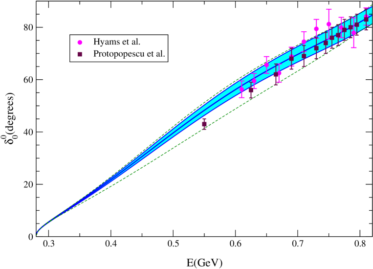
Figure 7: $I=0$ $S$–wave phase shift. The full line results with the central values of the scattering lengths and of the experimental input used in the Roy equations. The shaded region corresponds to the uncertainties of the result. The dotted lines indicate the boundaries of the region allowed if the constraints imposed by chiral symmetry are ignored [6]. The data points are from refs. [49] and [50].

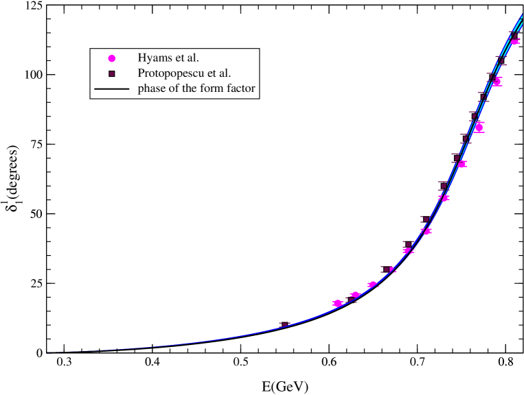
Figure 8: $P$–wave phase shift. The phase of the pion form factor is also shown, but it can barely be distinguished from the central result of our analysis. The data points are from refs. [49] and [50].

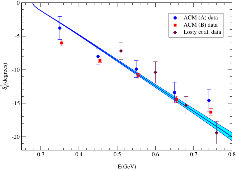
Figure 9: $I=2$ $S$–wave phase shift. The full line results with the central values of the scattering lengths and of the experimental input used in the Roy equations. The shaded region corresponds to the uncertainties of the result. The data points represent the two phase shift representations of the Aachen-Cern-Munich collaboration [51] and the one of Losty et al. [52]

For the reasons discussed in detail in ref. [6], the two $S$–wave scattering lengths are the essential parameters in the low energy domain. The result in eq. (11.2) specifies these to within very small uncertainties. In particular, we can now work out the phase shifts of the $S$– and $P$–waves on this basis, using the Roy equation analysis of [6]. The available experimental information for the imaginary parts above $\sqrt{s_{0}}=0.8\,\mbox{GeV}$, as well as the scattering lengths $a_{0}^{0}$, $a_{0}^{2}$ are used as an input, while the output of the calculation consists of the phases $\delta_{0}^{0}(s)$, $\delta_{1}^{1}(s)$ and $\delta_{0}^{2}(s)$, in the region below $s_{0}$. In view of the two subtractions occurring in the Roy equations, the behaviour of the imaginary parts above 1 GeV has very little influence on the behaviour of the solutions below $0.8\,\mbox{GeV}$. Also, there is a consistency check: In the region above $s_{0}$, the output must agree with the input. For the values of the scattering lengths required by chiral symmetry, this condition is indeed met. In fact, the solution of the Roy equations closely follow the input, within the rather broad range of variations allowed for the imaginary parts in ref. [6]. This also means that the Roy equations do not strongly constrain the behaviour of the phases above 0.8 GeV.

The result is shown in figs. 7, 8 and 9. For comparison, these figures also show the data points of the phase shift analyses given by Hyams et al. [49], Protopopescu et al. [50], the solutions A and B of Hoogland et al. (ACM) [51] and the one of Losty et al. [52], as well as the $P$–wave phase extracted from the data on the reactions $e^{+}e^{-}\rightarrow\pi^{+}\pi^{-}$ and $\tau\rightarrow\nu\pi\pi$. For further information on the $S$–wave phase shifts, we refer the reader to [53, 54].

The three central curves are described by the parametrization [55]

$$\tan\delta_{\ell}^{I}=\sqrt{1-{4M_{\pi}^{2}\over s}}\;q^{2\,\ell}\left\{A^{I}_{\ell}+B^{I}_{\ell}q^{2}+C^{I}_{\ell}q^{4}+D^{I}_{\ell}q^{6}\right\}\left({4M_{\pi}^{2}-s^{I}_{\ell}\over s-s^{I}_{\ell}}\right)\;,$$ (17.1)

with $s=4\,(M_{\pi}^{2}+q^{2})$. The numerical values of the coefficients are:

$$A_{0}^{0} \!\!\!= \!\!\!.220\,,\hskip 45.00006ptA^{1}_{1}=.379\cdot 10^{-1}\,,\hskip 22.0ptA^{2}_{0}=-.444\cdot 10^{-1}\,,$$

$$B_{0}^{0} \!\!\!= \!\!\!.268\,,\hskip 45.00006ptB^{1}_{1}=.140\cdot 10^{-4}\,,\hskip 20.00003ptB^{2}_{0}=-.857\cdot 10^{-1}\,,$$ (17.2)

$$C_{0}^{0} \!\!\!= \!\!\!-.139\cdot 10^{-1}\,,\hskip 10.00002ptC^{1}_{1}=-.673\cdot 10^{-4}\,,\hskip 13.00005ptC^{2}_{0}=-.221\cdot 10^{-2}\,,$$

$$D_{0}^{0} \!\!\!= \!\!\!-.139\cdot 10^{-2}\,,\hskip 10.00002ptD^{1}_{1}=.163\cdot 10^{-7}\,,\hskip 20.00003ptD^{2}_{0}=-.129\cdot 10^{-3}\,,$$

in units of $M_{\pi}$. In particular, the constants $A_{\ell}^{I}$ represent the scattering lengths of the three partial waves under consideration, while the $B_{\ell}^{I}$ are related to the effective ranges.

The parameters $s_{\ell}^{I}$ specify the value of $s$ where $\delta_{\ell}^{I}(s)$ passes through $90^{\circ}$:

$$s_{0}^{0}=36.77\,M_{\pi}^{2}\,,\hskip 10.00002pts^{1}_{1}=30.72\,M_{\pi}^{2}\,,\hskip 10.00002pts^{2}_{0}=-21.62\,M_{\pi}^{2}\,.$$ (17.3)

In the channels with $I=0,1$, the corresponding energies are $846\,\mbox{MeV}$ and $774\,\mbox{MeV}$, respectively (the negative sign of $s_{0}^{2}$ indicates that in the $I=2$ channel, which is exotic, the phase remains below $90^{\circ}$).

The value of the phase difference $\delta^{0}_{0}-\delta^{2}_{0}$ at $s=M_{K}^{2}$ is of special interest, in connection with the decays $K\rightarrow\pi\pi$. In particular, the phase of $\epsilon^{\prime}/\epsilon$ is determined by that phase difference. Our representation of the scattering amplitude allows us to pin this quantity down at the 3% level of acuracy:

$$\delta_{0}^{0}(M_{K^{0}}^{2})-\delta^{2}_{0}(M_{K^{0}}^{2})=47.7^{\circ}\pm 1.5^{\circ}\,.$$ (17.4)

We add two remarks concerning the comparison with the $P$–wave phase shift extracted from the $e^{+}e^{-}$ and $\tau$ data. First, we note that the agreement at 0.8 GeV is enforced by our approach: In the Roy equation analysis, the value of the phase shift at that energy represents an input parameter and we have made use of those data to pin it down. Once that is done, however, the behaviour of the phase shift at lower energies is unambiguously fixed: Chiral symmetry determines the two subtraction constants, so that the solution of the Roy equations becomes unique. In other words – disregarding the small effects due to the uncertainties in the input of our analysis, which are shown in fig. 8 – there is only one interpolation between threshold and 0.8 GeV that is consistent with the constraints imposed by analyticity, unitarity and chiral symmetry. Figure 8 shows that the predicted curve indeed very closely follows the phase extracted from the $e^{+}e^{-}$ and $\tau$ data. This confirms the conclusions reached in ref. [56].

Actually, the figure conceals a discrepancy in the threshold region, where the phase is too small for the effect to be seen by eye: Evaluating the $P$–wave scattering length with the Gounaris–Sakurai parametrization of the form factor given in ref. [57] (the curve shown in the figure), we obtain a result that is smaller than the value for $a_{1}^{1}$ in table 2, by about 10%, that is by many standard deviations of our prediction. The discrepancy is in the noise of the data on the form factor: There is little experimental information in the threshold region, so that the behaviour of the form factor is not strongly constrained there. Indeed, there are alternative parametrizations that also fit the data, but have a distinctly different behaviour near and below threshold. Even parametrizations with unphysical singularities at $s=0$, such as the one proposed in [58], provide decent fits in the experimentally accessible region. In this respect, the present work does add significant information about the $P$–wave phase shift, as it predicts the behaviour near threshold, within very narrow limits.

18 Poles on the second sheet

The partial wave amplitude $t^{1}_{1}(s)$ contains a pole on the second sheet. Denoting the pole position by $s=(M_{\rho}-\frac{i}{2}\,\Gamma_{\rho})^{2}$, we obtain

$$M_{\rho}=762.4\pm 1.8\,\mbox{MeV}\,,\hskip 10.00002pt\Gamma_{\rho}=145.2\pm 2.8\,\mbox{MeV}\,.$$ (18.1)

Note that the values quoted for the “mass” often represent the energy where the real part of the amplitude vanishes – in contrast to the position of the pole, that value is not independent of the process considered. As the scattering is approximately elastic there, the corresponding mass is the energy where the phase shift goes through $90^{\circ}$. For the $P$–wave, this happens at

$$m_{\rho}=773.5\pm 2.5\,\mbox{MeV}\,.$$

The real part of the pole position is smaller than the energy where the phase shift passes through $90^{\circ}$, by about 10 MeV. The uncertainty in $\Gamma_{\rho}$ is significantly smaller than the error bar quoted in [6]: The constraints imposed on the scattering amplitude by the low energy theorems of chiral symmetry also allow a better determination of the width.

The $I=0$ $S$–wave also contains a pole on the second sheet. The uncertainties in the pole position are considerably larger than in the case of the $\rho$, because the singularity is far from the real axis. Also, the uncertainties in the phase shift are somewhat larger here. Varying the input parameters as well as the analytic form of the representation used for $t_{0}^{0}$, we find that the pole occurs in the region $\sqrt{s}=(470\pm 30)-\,i\,(295\pm 20)\,\mbox{MeV}$, while the phase passes through $90^{\circ}$ at $\sqrt{s}=844\pm 13\,\mbox{MeV}$.

There is no harm in calling this an unusually broad resonance, but that sheds little light on the low energy structure of the scattering amplitude. In particular, it should not come as a surprise if the values for the mass and width of the resonance, obtained on the basis of the assumption that the pole represents the most important feature in this channel, are very different from the real and imaginary parts of the energy at which the amplitude actually has a pole – there is more to the physics of the $S$–wave than the occurrence of a pole far from the real axis. A collection of numbers concerning the pole position is given in [59] and for a recent review of the abundant literature on the subject, we refer to [60]. A recent discussion in the framework of the $NN$ interaction is given in [61].

We add a remark concerning the physics behind the pole in $t^{0}_{0}$ – admittedly, the reasoning is of qualitative nature. In the chiral limit, current algebra predicts $t^{0}_{0}=s/16\pi F_{\pi}^{2}$: The amplitude vanishes at threshold, but the real part grows quadratically with the energy, so that the imaginary part rises with the fourth power. The rapid growth signals the occurrence of a strong final state interaction. In order to estimate the strength of the corresponding branch cut, we invoke the inverse amplitude method, replacing the above formula by $t_{0}^{0}=s/(16\pi F_{\pi}^{2}-i\,s)$. The virtue of this operation is that, while it retains the algebraic accuracy of the current algebra approximation, it yields an expression that does obey elastic unitarity. The formula shows that, in this approximation, the amplitude contains a pole at $\sqrt{s}=\sqrt{-i\,16\,\pi}\,F_{\pi}=463-i\,463\,\mbox{MeV}$, indeed not far away from the place where the full amplitude has a pole.

The physics of the $P$–wave is very different, because the unitarity cut generated by low energy $\pi\pi$ intermediate states is very weak. Repeating the above exercise for $t^{1}_{1}$, one again finds a pole with equal real and imaginary parts, but it is entirely fictitious, as it occurs at $1.1-i\,1.1$ GeV, far beyond the region where current algebra provides a meaningful approximation. The occurrence of a pole near the real axis cannot be understood on the basis of chiral symmetry and unitarity alone.

In the framework of the effective theory, the difference manifests itself as follows. While the unitarity corrections account perfectly well for the low energy behaviour of the imaginary parts, the presence of the $\rho$ only shows up in the values of the effective coupling constants $\ell_{1},\ell_{2}$ and $\ell_{6}$. There is no such pole in $t^{1}_{1}$, for instance, if the underlying theory is identified with the linear $\sigma$–model, and the values of those coupling constants are then very different [9]. In this sense, the pole in $t^{1}_{1}$ reflects a special property of QCD, while the one in $t^{0}_{0}$ can be understood on the basis of the fact that chiral symmetry predicts a strong unitarity cut: The pole position is related to the magnitude of $F_{\pi}$.

19 Threshold parameters

	A	B	C	D	E	units
$a_{0}^{0}$	$.220\pm.005$	$.216$	$.220\pm.005$	$.24\pm.06$	$.26\pm.05$
$b^{0}_{0}$	$.276\pm.006$	$.268$	$.280\pm.011$	$.26\pm.02$	$.25\pm.03$	$M_{\pi}^{-2}$
$a_{0}^{2}$	$-.444\pm.010$	$-.445$	$-.423\pm.010$	$-.36\pm.13$	$-.28\pm.12$	$10^{-1}$
$b_{0}^{2}$	$-.803\pm.012$	$-.808$	$-.762\pm.021$	$-.79\pm.05$	$-.82\pm.08$	$10^{-1}M_{\pi}^{-2}$
$a_{1}^{1}$	$.379\pm.005$	$.380$	$.380\pm.021$	$.37\pm.02$	$.38\pm.02$	$10^{-1}M_{\pi}^{-2}$
$b_{1}^{1}$	$.567\pm.013$	$.537$	$.58\pm.12$	$.54\pm.04$		$10^{-2}M_{\pi}^{-4}$
$a^{0}_{2}$	$.175\pm.003$	$.176$	$.22\pm.04$	$.17\pm.01$	$.17\pm.03$	$10^{-2}M_{\pi}^{-4}$
$b_{2}^{0}$	$-.355\pm.014$	$-.343$	$-.32\pm.10$	$-.35\pm.06$		$10^{-3}M_{\pi}^{-6}$
$a^{2}_{2}$	$.170\pm.013$	$.172$	$.29\pm.10$	$.18\pm.08$	$.13\pm.3$	$10^{-3}M_{\pi}^{-4}$
$b_{2}^{2}$	$-.326\pm.012$	$-.339$	$-.36\pm.9$	$-.34\pm.07$		$10^{-3}M_{\pi}^{-6}$
$a_{3}^{1}$	$.560\pm.019$	$.545$	$.61\pm.11$	$.58\pm.12$	$.6\pm.2$	$10^{-4}M_{\pi}^{-6}$
$b_{3}^{1}$	$-.402\pm.018$	$-.312$	$-.36\pm.02$	$-.44\pm.14$		$10^{-4}M_{\pi}^{-8}$

Table 2: Threshold parameters. Our results are listed in column A. The numbers in the next two columns are obtained by evaluating the chiral representation at threshold: The entries under B follow from our values of the effective coupling constants, while those under C are taken from ref. [22]. Column D gives the outcome of a Roy equation analysis that does not invoke chiral symmetry [6], while E contains the old “experimental” values [27].

The scattering lengths of the partial waves with $\ell\geq 1$, as well as the effective ranges (also of those of the $S$–waves) can be expressed in terms of sum rules over the imaginary parts [62]. The corresponding numerical values are listed in the table 2, together with the $S$–wave scattering lengths. Column A indicates our final results, obtained by matching the phenomenological and chiral representations in the subthreshold region and using the Roy equations to evaluate the amplitude and its derivatives at threshold. In column B, we quote the numbers obtained from a direct evaluation of the two loop representation at threshold, using our central values for the effective coupling constants – this amounts to truncating the expansion of the threshold parameters in powers of $m_{u}$ and $m_{d}$. Column C lists the results of ref. [22], where the amplitude is also expanded at threshold, but the coupling constants are determined on the basis of a two loop analysis of the $K_{e4}$ form factors (see the next section for a comment concerning these entries). The comparison of the columns A, B and C clearly shows that two loop chiral perturbation theory works very well in describing both $\pi\pi$ scattering and $K_{e4}$ decays. For the reasons given in section 9, the method described in the present paper yields the smallest error bars. In fact, it is quite remarkable that the results for the effective range $b_{3}^{1}$ in columns B and C represent a decent estimate: In this case, only the infrared singularities occurring in the expansion in powers of the quark masses contribute. For comparison, column D lists the values of ref. [6], which are obtained by analyzing the available data with the Roy equations and do not invoke chiral perturbation theory. Finally, column E contains the values of the compilation in refs. [27].

20 Quark mass dependence of $M_{\pi}^{2}$ and $F_{\pi}$

The dependence of physical quantities on the quark masses is of interest, in particular, for the following reason: By now, dynamical quarks with a mass of the order of the physical value of $m_{s}$ are within reach on the lattice, but it is notoriously difficult to equip the two lightest quarks with their proper masses. Invariably, the numerical results obtained for the physical values of $m_{u}$ and $m_{d}$ rely on an extrapolation of numerical data. For a recent, comprehensive review of lattice work on the light quark masses, we refer to [63].

In this connection, chiral perturbation theory may turn out to be useful, because it predicts the mass dependence in terms of a few constants: the coupling constants of the effective Lagrangian. Above, we have determined some of these and we now discuss the consequences for the dependence of $M_{\pi}^{2},F_{\pi},a_{0}^{0},a_{0}^{2}$ on the masses of the two lightest quarks: We keep $m_{s}$ fixed at the physical value and set $m_{u}=m_{d}=m$, but vary the value of $m$ in the range $0<m<\frac{1}{2}\,m_{s}$ (at the upper end of that range, the pion mass is about 500 MeV).

In the preceding sections, we have expressed all of the quantities in terms of the physical pion mass and the physical decay constant, using the ratio $\xi$ as an expansion parameter. Also, the logarithmic infrared singularities were normalized at the scale $M_{\pi}$. In particular, the coupling constants $\,\overline{\rule[7.5pt]{3.99994pt}{0.0pt}}\ell_{n}$ contain a chiral logarithm with unit coefficient, so that they may be represented as

$$\,\overline{\rule[7.5pt]{3.99994pt}{0.0pt}}\ell_{n}\equiv\ln\frac{\Lambda_{n}^{\,2}}{M_{\pi}^{2}}\,,$$ (20.1)

where $\Lambda_{n}$ is the intrinsic scale of $\ell_{n}$ and is independent both of $m$ and of the running scale $\mu$. In order to explicitly exhibit the quark mass dependence, we replace $M_{\pi}^{2}$ by the variable $M^{2}\equiv 2\,m\,B$ and also normalize the chiral logarithms at the scale $M$, trading the quantities $\xi$ and $\,\overline{\rule[7.5pt]{3.99994pt}{0.0pt}}\ell_{n}$ for

$$x\equiv\frac{M^{2}}{16\,\pi^{2}F^{2}}\,,\hskip 20.00003pt\hat{\ell}_{n}\equiv\ln\frac{\Lambda_{n}^{\;2}}{M^{2}}\,,$$ (20.2)

respectively. According to (7.1), (7.2) the two sets of variables are related by

$$x \!\!\!= \!\!\!\xi\{1+\mbox{$\frac{1}{2}$}\,\xi\,(\,\overline{\rule[7.5pt]{3.99994pt}{0.0pt}}\ell_{3}+4\,\overline{\rule[7.5pt]{3.99994pt}{0.0pt}}\ell_{4})+O(\xi^{2})\}\,,\hskip 20.00003pt\hat{\ell}_{n}=\,\overline{\rule[7.5pt]{3.99994pt}{0.0pt}}\ell_{n}-\mbox{$\frac{1}{2}$}\,\xi\,\,\overline{\rule[7.5pt]{3.99994pt}{0.0pt}}\ell_{3}+O(\xi^{2})$$ (20.3)

$$\xi \!\!\!= \!\!\!x\{1-\mbox{$\frac{1}{2}$}\,x\,(\hat{\ell}_{3}+4\hat{\ell}_{4})+O(x^{2})\}\,,\hskip 18.00005pt\,\overline{\rule[7.5pt]{3.99994pt}{0.0pt}}\ell_{n}=\hat{\ell}_{n}+\mbox{$\frac{1}{2}$}\,x\,\hat{\ell}_{3}+O(x^{2})\,.$$

The expansions of $M_{\pi}^{2}$ and $F_{\pi}$ in powers of $m$ are known to next–to–next–to–leading order [64, 65, 5]. In the above notation, the explicit expressions may be written in the form [66]:

$$M_{\pi}^{2} \!\!\!= \!\!\!M^{2}\,\{1-\mbox{$\frac{1}{2}$}\,x\,\hat{\ell}_{3}+\mbox{$\frac{17}{8}$}\,x^{2}\hat{\ell}_{\!\scriptscriptstyle M}^{\;2}+x^{2}k_{\scriptscriptstyle M}+O(x^{3})\,,$$

$$F_{\pi} \!\!\!= \!\!\!F\,\{1+x\,\hat{\ell}_{4}-\mbox{$\frac{5}{4}$}\,x^{2}\hat{\ell}_{\!\scriptscriptstyle F}^{\;2}+x^{2}k_{\scriptscriptstyle F}+O(x^{3})\,,$$

$$\hat{\ell}_{\!\scriptscriptstyle M} \!\!\!= \!\!\!\frac{1}{51}\,(28\,\hat{\ell}_{1}+32\,\hat{\ell}_{2}-9\,\hat{\ell}_{3}+49)\,,$$ (20.4)

$$\hat{\ell}_{\!\scriptscriptstyle F} \!\!\!= \!\!\!\frac{1}{30}\,(14\,\hat{\ell}_{1}+16\,\hat{\ell}_{2}+6\,\hat{\ell}_{3}-6\,\hat{\ell}_{4}+23)\,,$$

In this representation, the infrared singularities are hidden in the scale invariant quantities $\hat{\ell}_{1},\ldots\,,\hat{\ell}_{4}$. Those generated by the two loop graphs have been completed to a square. The normalization of the auxiliary quantities $\hat{\ell}_{\!\scriptscriptstyle M}$, $\hat{\ell}_{\!\scriptscriptstyle F}$ is chosen such that their mass dependence is also of the form

$$\hat{\ell}_{\!\scriptscriptstyle M}=\ln\frac{\Lambda_{\!\scriptscriptstyle M}^{\,2}}{M^{2}}\,,\hskip 20.00003pt\hat{\ell}_{\!\scriptscriptstyle F}=\ln\frac{\Lambda_{\!\scriptscriptstyle F}^{\,2}}{M^{2}}\,.$$ (20.5)

The constants $k_{\!\scriptscriptstyle M}$, $k_{\!\scriptscriptstyle F}$ collect the analytic contributions at order $x^{2}$ and are independent of $m$ and $\mu$. By completing the logarithms at oder $x^{2}$ to a square, we have in effect chosen a particular running scale: the one where the coefficient of the term linear in $\ln M^{2}$ vanishes. This simplifies the representation, but is without physical significance – the decomposition into an infrared singular part arising from the Goldstone bosons and a regular remainder is not unique. In ref. [21], a somewhat different representation for the analytic terms of order $x^{2}$ is used, which involves the two parameters $r_{\scriptscriptstyle M}$, $r_{\scriptscriptstyle F}$ instead of $k_{\!\scriptscriptstyle M}$, $k_{\!\scriptscriptstyle F}$.

21 Numerical results for quark mass dependence

In addition to the coupling constants $\ell_{1},\ldots,\ell_{4}$ that also govern the low energy properties of the $\pi\pi$ scattering amplitude, the ratios $M_{\pi}^{2}/M^{2}$ and $F_{\pi}/F$ contain the two fourth order constants $k_{\!\scriptscriptstyle M}$ and $k_{\!\scriptscriptstyle F}$. We expect that the contributions from these terms are of order $M_{\pi}^{4}/M_{\scriptscriptstyle S}^{4}$ and can just as well be dropped – unless $m$ is taken much larger than in nature. We did not make an attempt at quantifying the uncertainties associated with these terms, because they are small compared to those from the coupling constants $\ell_{1},\ldots,\ell_{4}$. The bands shown in fig. 10 correspond to $r_{\scriptscriptstyle M}=r_{\scriptscriptstyle F}=0$. If we were to instead set the constants $k_{\!\scriptscriptstyle M}$, $k_{\!\scriptscriptstyle F}$ equal to zero, the boundaries would be slightly shifted, but the shifts are small compared to the width of the bands.

For small values of $m$, the contributions of $O(m^{2})$ dominate. These are determined by the two scales $\Lambda_{3}$ and $\Lambda_{4}$. As discussed in section 7, the information about the first one is meagre – the crude estimate (7.8) amounts to $0.2\,\mbox{GeV}<\Lambda_{3}<2\,\mbox{GeV}$. For the second one, however, the value for $\,\overline{\rule[7.5pt]{3.99994pt}{0.0pt}}\ell_{4}$ obtained in section 11 yields a rather decent determination:

$$\Lambda_{4}=1.26\pm 0.14\,\mbox{GeV}\,.$$ (21.1)

The two parameters $\Lambda_{3},\Lambda_{4}$ play the same role as the coefficients $c_{\scriptscriptstyle M}$ and $c_{\scriptscriptstyle F}$ in the polynomial approximations $M_{\pi}^{2}=2\,mB\,(1+c_{\scriptscriptstyle M}\,m)$, $F_{\pi}=F\,(1+c_{\scriptscriptstyle F}\,m)$, that are sometimes used to perform the extrapolation of lattice data. In contrast to these approximations, the formulae (20) do account for the infrared singularities of the functions $M_{\pi}(m)$ and $F_{\pi}(m)$ – to the order of the expansion in powers of $m$ considered, that representation is exact.

Consider first the ratio $F_{\pi}/F$, for which the poorly known scale $\Lambda_{3}$ only enters at next–to–next–to–leading order. The upper one of the two shaded regions in fig. 10 shows the behaviour of this ratio as a function of $M$, according to formula (20). The change in $F_{\pi}$ occurring if $M$ is increased from the physical value to $M_{K}$ is of the expected size, comparable to the difference between $F_{K}$ and $F_{\pi}$. The curvature makes it evident that a linear extrapolation in $m$ is meaningless. The essential parameter here is the scale $\Lambda_{4}$ that determines the magnitude of the term of order $M^{2}$. The corrections of order $M^{4}$ are small – the scale relevant for these is $\Lambda_{F}\simeq 0.5\,\mbox{GeV}$.

Figure 10: Dependence of the ratios $F_{\pi}/F$ and $M_{\pi}^{2}/M^{2}$ on the mass of the two lightest quarks. The variable $M$ is defined by $M^{2}=(m_{u}+m_{d})\,B$ and $F$ is the value of the pion decay constant for $m_{u}=m_{d}=0$. The strange quark mass is held fixed at the physical value.

In the case of the ratio $M_{\pi}^{2}/M^{2}$, on the other hand, the dominating contribution is determined by the scale $\Lambda_{3}$ – the corrections of $O(M^{4})$ are small also in this case (the relevant scale is $\Lambda_{M}\simeq 0.6\,\mbox{GeV}$). The fact that the information about the value of $\ell_{3}$ is very meagre shows up through very large uncertainties. In particular, with $\Lambda_{3}\simeq 0.5\,\mbox{GeV}$, the ratio $M_{\pi}^{2}/M^{2}$ would remain very close to 1, on the entire interval shown. Note that outside the range of values for $\ell_{3}$ considered in the present paper, the dependence of $M_{\pi}^{2}$ on the quark masses would necessarily exhibit strong curvature. This is illustrated with the dashed line that indicates the behaviour of the ratio $M_{\pi}^{2}/M^{2}$ for $\,\overline{\rule[7.5pt]{3.99994pt}{0.0pt}}\ell_{3}=-10$. According to fig. 2 this value corresponds to $a_{0}^{0}\simeq 0.24$.

The above discussion shows that brute force is not the only way to reach the very small values of $m_{u}$ and $m_{d}$ observed in nature on the lattice. It suffices to equip the strange quark with the physical value of $m_{s}$ and to measure the dependence of the pion mass on $m_{u},m_{d}$ in the region where $M_{\pi}$ is comparable to $M_{K}$. Since the dependence on the quark masses is known rather accurately in terms of the two constants $B$ and $\Lambda_{3}$, a fit to the data based on eq. (20) should provide an extrapolation to the physical quark masses that is under good control. Moreover, the resulting value for $\Lambda_{3}$ would be of considerable interest, because that scale also shows up in other contexts, in the $\pi\pi$ scattering lengths, for example. For recent lattice work in this direction, we refer to [67]. A measurement of the mass dependence of $F_{\pi}$ in the same region would be useful too, because it would provide a check on the dispersive analysis of the scalar radius that underlies our determination of $\Lambda_{4}$ – in view of the strong unitarity cut in the scalar form factor, a direct evaluation of the scalar radius on the lattice is likely more difficult. Chiral logarithms also occur in the quenched approximation [68, 69], but since the coefficients differ from those in the full theory, a naive comparison of the above formulae with quenched lattice data is not meaningful.

Figure 11: Size of the corrections to Weinberg’s leading order predictions for the $\pi\pi$ $S$–wave scattering lengths, as a function of the pion mass.

In section 9, we noted that the expansion of the scattering length $a_{0}^{0}$ in powers of the quark mass contains an unusually large infrared singularity at one loop level. We can now complete that discussion with an evaluation of the contributions arising at next–to–next–to–leading order, repeating the analysis of ref. [70] with the information about the coupling constants available now. The result is shown in figure 11, where we indicate the behaviour of the correction factors $R_{0},R_{2}$, defined by

$$a_{0}^{0}=\frac{7\,M_{\pi}^{2}}{32\,\pi F_{\pi}^{2}}\,R_{0}\,,\hskip 20.00003pta_{0}^{2}=-\frac{M_{\pi}^{2}}{16\,\pi F_{\pi}^{2}}\,R_{2}\,,$$

as a function of $M_{\pi}$. The reason for choosing the variable $M_{\pi}$ rather than $M$ is that the uncertainties in $\Lambda_{3}$ then affect the result less strongly. The comparison with figure 10, where a larger mass range is shown, demonstrates that $R_{0}$ grows much more rapidly with the quark masses than $F_{\pi}$. The effect arises from the chiral logarithms associated with the unitarity cut – the coefficient of the leading infrared singularity in $a_{0}^{0}$ exceeds the one in $F_{\pi}$ by a factor $\frac{9}{2}$. Note that the chiral perturbation theory formulae underlying the figure are meaningful only in the range where the corrections are small. The shaded regions exclusively account for the uncertainties in the values of the coupling constants. In the case of $R_{0}$, those due to the terms of order $M_{\pi}^{6}$ are by no means negligible for $M_{\pi}>0.2\,\mbox{GeV}$, so that it matters what exactly is plotted. The curves shown in the figure are obtained by expressing $R_{0}$, $R_{2}$ in terms of the coupling constants $F,\,\ell_{1},\ldots$ and of $M_{\pi}$, expanding the result in powers of $M_{\pi}$ and truncating the series at order $M_{\pi}^{4}$. On the left half of the figure, the behaviour of $R_{0}$ obtained, for instance, by truncating the expansion in powers of $M$ instead of the one in $M_{\pi}$ is practically the same, but on the right half, there is a substantial difference, indicating that the chiral perturbation series is out of control there.

We conclude that in the case of the $I=0$ scattering length, a meaningful extrapolation of lattice data to the physical values of $m_{u}$ and $m_{d}$ requires significantly smaller quark masses than in the case of $M_{\pi}$ or $F_{\pi}$. In the $I=2$ channel, the effects are much smaller, because this channel is exotic: The final state interaction is weak and repulsive. The lattice result, $a_{0}^{2}=-0.0374\pm 0.0049$ [71], corresponds to $R_{2}=0.82\pm 0.11$. It is on the low side, but not inconsistent with our prediction: $a_{0}^{2}=-0.0444\pm 0.0010$, $R_{2}=0.98\pm 0.02$. As in the case of $F_{\pi}$ and $M_{\pi}$, the comparison between the lattice result and our prediction is not really meaningful, because that result relies on the quenched approximation. The evaluation of the scattering lengths to one loop in the quenched approximation [69, 72] has shown that the infrared singularities are different from those in full QCD. Moreover, as pointed out by Bernard and Golterman [72], the very method used to extract the infinite volume scattering lengths from finite volume observables [73] is affected: In addition to the purely statistical error, the numbers in [71] have a sizeable systematic error.

22 Summary and conclusion

  1. The Roy equations determine the $\pi\pi$ scattering amplitude in terms of the imaginary parts at intermediate energies, except for two subtraction constants: the $S$–wave scattering lengths $a_{0}^{0}$, $a_{0}^{2}$. At low energies, the contributions from the imaginary parts are small, so that the current experimental information about these suffices, but the one about the scattering lengths is subject to comparatively large uncertainties.

2. The low energy theorems of chiral symmetry provide the missing element: They predict the values of the two subtraction constants. In the chiral limit, where the pions are massless, the $S$–wave scattering lengths vanish. The breaking of the symmetry generated by the quark masses $m_{u}$ and $m_{d}$ leads to nonzero values, for $M_{\pi}$ as well as for $a_{0}^{0}$ and $a_{0}^{2}$. The Gell-Mann-Oakes-Renner relation (1.1) shows that the leading term in the expansion of $M_{\pi}^{2}$ in powers of the quark masses is determined by the quark condensate and by the pion decay constant. Weinberg’s low energy theorems (1.2) demonstrate that the same two constants also determine the leading term in the expansion of the scattering lengths. Ignoring the higher order contributions, these relations predict $a_{0}^{0}=0.159$, $a_{0}^{2}=-.0454$.

3. Chiral perturbation theory allows us to analyze the higher order terms of the expansion in a systematic manner. In the isospin limit, $m_{u}=m_{d}=m$, the perturbation series of the $\pi\pi$ scattering amplitude has been worked out to next–to–next–to–leading order (two loops). The result, in particular, specifies the expansion of $a_{0}^{0}$ and $a_{0}^{2}$ in powers of $m$ up to and including $O(m^{3})$. The isospin breaking effects due to $m_{u}\neq m_{d}$ have also been been studied [74]. These effects only show up at nonleading orders of the expansion and are small – in contrast to the kaons or the nucleons, the pions are protected from isospin breaking. In the present paper, we have ignored these effects altogether.

4. Chiral symmetry does not fully determine the higher order contributions, because it does not predict the values of the coupling constants occurring in the effective Lagrangian. There are two categories of coupling constants: terms that survive in the chiral limit and symmetry breaking terms proportional to a power of $m$. The former show up in the momentum dependence of the scattering amplitude, so that these couplings can be determined phenomenologically. For the coupling constants of the second category, which describe the dependence on the quark masses, we need to rely on sources other than $\pi\pi$ scattering.

5. The higher order terms of the expansion are dominated by those of next–to–leading order, which involve the coupling constants $\ell_{1}$, $\ell_{2}$ from the first category and $\ell_{3}$, $\ell_{4}$ from the second. We rely on the dispersive analysis of the scalar pion form factor to pin down the coupling constant $\ell_{4}$. Crude theoretical estimates indicate that the contributions from $\ell_{3}$ are very small, but the uncertainties of these estimates dominate the error in our final result for the $S$–wave scattering lengths. We also rely on theoretical estimates for the symmetry breaking coupling constants $r_{1},\ldots,,r_{4}$ of next–to–next–to–leading order. These indicate that the contributions to $a_{0}^{0}$ and $a_{0}^{2}$ from those constants are tiny and could just as well be dropped.

6. The expansion in powers of the quark masses contains infrared singularities – the chiral logarithms characteristic of chiral perturbation theory. In the case of $a_{0}^{0}$, for instance, these singularities enhance the magnitude of the corrections quite substantially. The origin of the phenomenon is well understood: The final state interaction in the $I=0$ $S$–wave generates a strong branch cut. For this reason, the straightforward expansion of $a_{0}^{0}$ in powers of $m$ converges only rather slowly. We exploit the fact that, in the subthreshold region, the expansion of the scattering amplitude converges much more rapidly: In our approach, the chiral and phenomenological representations of the scattering amplitude are matched there. With this method, even the one loop approximation of the chiral perturbation series yields values for the scattering lengths that are within the errors of our final result, which reads

$$\!\!\!a_{0}^{0}=0.220\pm 0.005\,,\hskip 52.00005pta^{2}_{0}=-0.0444\pm 0.0010\,,$$

$$\!\!\!2a_{0}^{0}-5a_{0}^{2}=0.663\pm 0.007\,,\hskip 20.00003pta^{0}_{0}-a^{2}_{0}=0.265\pm 0.004\,.$$

7. We have worked out the implications for the phase shifts of the $S$– and $P$–waves. As shown in figs. 7–9, chiral symmetry and the existing experimental information constrain these to a rather narrow range. The corresponding predictions for the scattering lengths of the $D$– and $F$–waves, as well as for the effective ranges are listed in table 2.

8. Our representation of the scattering amplitude, in particular, also yields an accurate prediction for the phase of $\epsilon^{\prime}/\epsilon$: The result for the phase difference between the two $S$–waves at $s=M_{K^{0}}^{2}$ reads

$$\delta^{0}_{0}(M_{K^{0}}^{2})-\delta^{2}_{0}(M_{K^{0}}^{2})=47.7^{\circ}\pm 1.5^{\circ}\,.$$ (22.1)

9. The mass and the width of the $\rho$–meson can be calculated to within remarkably small uncertainties:

$$M_{\rho} \!\!\!= \!\!\!762.4\pm 1.8\,\mbox{MeV}\,,\hskip 20.00003pt\Gamma_{\rho}=145.7\pm 2.6\,\mbox{MeV}\,.$$ (22.2)

Also, we confirm that the $I=0$ $S$–wave contains a pole far away from the real axis, at $\sqrt{s}=(470\pm 30)-i\,(295\pm 20)\,\mbox{MeV}$. The phenomenon is related to the fact that chiral symmetry requires the scattering amplitude to be very small at threshold and then to grow with the square of the energy.

10. The consequences for the coupling constants $\ell_{1}$, $\ell_{2}$, $\ell_{4}$, $r_{5}$ and $r_{6}$ of the effective Lagrangian were studied in detail. Our results are in good agreement with previous work, but are more accurate. In particular, we have shown that $\ell_{1}$ and $\ell_{2}$ are accompanied by strong infrared singularities generated by the two loop graphs, which shift the numerical values obtained in one loop approximation, quite substantially. The effective couplings relevant at one loop level are given in eq. (14.3). We have shown that, with these values, a very decent representation of the scattering amplitude is obtained by matching the Roy equations with the one loop approximation of chiral perturbation theory: The result can barely be distinguished from the representation that underlies the present paper.

11. The results for the various quantities of interest are strongly correlated. We have examined the correlations in detail, not only for the threshold parameters and coupling constants, but also for the coefficients $b_{1},\ldots\,,b_{6}$ of the polynomial that occurs in the chiral perturbation theory representation of the scattering amplitude.

12. The resulting picture for the low energy structure of the scattering amplitude is consistent with the resonance saturation hypothesis: For all of the effective coupling constants encountered in the two loop representation, our results are consistent with the assumption that, once the poles and cuts due to pion exchange are removed, the low energy structure of the amplitude is dominated by the singularities due to the lightest non–Goldstone states [9]. Since the splitting of a resonance contribution from the continuum underneath it is not unique, the saturation hypothesis does not lead to very sharp predictions, but it is by no means trivial that these are consistent with the values found, both in sign and magnitude.

13. On the lattice, it is difficult to reach the small values of $m_{u}$ and $m_{d}$ that are realized in nature. We have shown that chiral perturbation theory can be used to extrapolate the results obtained at comparatively large values for these masses, in a controlled manner. The method at the same time also allows a measurement of some of the coupling constants that occur in the symmetry breaking part of the effective Lagrangian, in particular, of $\ell_{3}$. In quite a few cases, the uncertainties in our results are dominated by those from this term.

14. We emphasize that most of our results rely on the standard picture, according to which the quark condensate represents the leading order parameter of the spontaneously broken symmetry, so that the Gell-Mann-Oakes-Renner relation holds. The crude theoretical estimates for the coupling constant $\ell_{3}$ we are relying on indicate that the higher order terms in the expansion of $M_{\pi}^{2}$ are very small, so that the square of the pion mass indeed grows linearly with $m=\frac{1}{2}\,(m_{u}+m_{d})$ – a curvature only shows up if $m$ is taken much larger than the physical value. In ref. [23], $\ell_{3}$ is instead treated as a free parameter and is allowed to take large values, so that the dependence of $M_{\pi}^{2}$ on the quark masses fails to be approximately linear, even in the region below the physical value of $m$. There is no prediction for the scattering lengths in that framework.

15. Even if the quark condensate is not assumed to represent the leading order parameter, a strong correlation between $a_{0}^{0}$ and $a_{0}^{2}$ emerges, which originates in the relation between these quantities and the scalar radius. The correlation is of interest, in particular, in connection with the analysis of $K_{e_{4}}$ data: As shown in fig. 3, the preliminary results of the E865 experiment at Brookhaven [29, 30] yield a remarkably good determination of $a_{0}^{0}$. The outcome beautifully confirms the prediction (11.2): The best fit to these data is obtained for $a_{0}^{0}=0.218$, with $\chi^{2}=5.7$ for 5 degrees of freedom. For a detailed discussion of the consequences for the value of $a_{0}^{0}$, we refer to [46, 47].

16. A measurement that aims at determining the lifetime of a $\pi^{+}\pi^{-}$ atom to an accuracy of 10% is currently under way at CERN. The interference of the electromagnetic and strong interaction effects in the bound state and in the decay is now well understood, also on the basis of chiral perturbation theory [35]. The decay rate of the ground state can be written in the form

$$\Gamma \!\!\!= \!\!\!\frac{2}{9}\,\alpha^{3}p\,|a_{0}^{0}-a_{0}^{2}|^{2}\,(1+\delta)\,,$$

with $p=\sqrt{M_{\pi^{+}}^{2}-M_{\pi^{0}}^{2}-\mbox{$\frac{1}{4}$}\,\alpha^{2}\,M_{\pi^{+}}^{2}}$. The term $\delta$ accounts for the corrections of order $\alpha$ as well as those due to $m_{u}\neq m_{d}$. According to ref. [35], these effects increase the rate by $\delta=0.058\pm 0.012$, that is by about 6%. Inserting our result (11.2) for $a_{0}^{0}-a_{0}^{2}$, we arrive at the following prediction for the lifetime [75]:

$$\tau=(2.90\pm 0.10)\cdot 10^{-15}\,\mbox{s}\,.$$ (22.3)

Since the decay rate is proportional to $|a_{0}^{0}-a_{0}^{2}|^{2}$, the outcome of the experiment is expected to lead to a determination of $|a_{0}^{0}-a_{0}^{2}|$ to an accuracy of 5%, thereby subjecting chiral perturbation theory to a very sensitive test.

Acknowledgement

We are indebted to S. Pislak and P. Truöl for providing us with preliminary data of the E865 collaboration, and we thank H. Bijnens and G. Wanders for informative discussions and comments. This work was supported in part by the Swiss National Science Foundation, and by TMR, BBW-Contract No. 97.0131 and EC-Contract No. ERBFMRX-CT980169 (EURODA$\Phi$NE).

Appendix A Notation

We use the following abbreviations:

$$\!\!\!\xi=\left(\frac{M_{\pi}}{4\pi F_{\pi}}\right)^{\!\!2}\,,\hskip 10.00002ptx=\left(\frac{M}{4\pi F}\right)^{\!\!2}\,,\hskip 10.00002pt\tilde{L}=\ln\frac{\mu^{2}}{M_{\pi}^{2}}\,,\hskip 10.00002ptN=16\pi^{2}\,.$$

The intrinsic scales of the coupling constants of ${\cal L}_{4}$ are denoted by $\Lambda_{n}$. In terms of these, the standard renormalized couplings are given by

$$\ell^{r}_{n}(\mu)=\frac{\gamma_{n}}{32\pi^{2}}\,\ln\frac{\Lambda_{n}^{\;2}}{\mu^{2}}\,,\hskip 20.00003pt\gamma_{1}=\mbox{$\frac{1}{3}$}\,,\hskip 10.00002pt\gamma_{2}=\mbox{$\frac{2}{3}$}\,,\hskip 10.00002pt\gamma_{3}=-\mbox{$\frac{1}{2}$}\,,\hskip 10.00002pt\gamma_{1}=2\,,$$

where $\mu$ is the running scale. The scales relevant in the various applications are different and the formulae can be simplified considerably if the coupling constants are normalized at the appropriate scale. For this reason, we use three different symbols:

$$\!\!\!\,\overline{\rule[7.5pt]{3.99994pt}{0.0pt}}\ell_{n}=\ln\frac{\Lambda_{n}^{\;2}}{M_{\pi}^{2}}\,,\hskip 20.00003pt\hat{\ell}_{n}=\ln\frac{\Lambda_{n}^{\;2}}{M^{2}}\,,\hskip 20.00003pt\tilde{\ell}_{n}=\ln\frac{\Lambda_{n}^{\;2}}{\mu^{2}}\,.$$

The first coincides with the one introduced in [4], in the framework of a one loop analysis, where there is no need to distinguish $\,\overline{\rule[7.5pt]{3.99994pt}{0.0pt}}\ell_{n}$ from $\hat{\ell}_{n}$. The quantities $\tilde{\ell}_{n}$ differ from the running coupling constants $\ell^{r}_{n}(\mu)$ only by a numerical factor, which it is convenient to remove in order to simplify the expressions. For the same reason, we work with the coefficients $\,\overline{\rule[7.20001pt]{3.99994pt}{0.0pt}}b_{1},\ldots\,,\,\overline{\rule[7.20001pt]{3.99994pt}{0.0pt}}b_{6}$, introduced in [5],

$$\,\overline{\rule[7.20001pt]{3.99994pt}{0.0pt}}b_{1}=Nb_{1}\,,\hskip 10.00002pt\,\overline{\rule[7.20001pt]{3.99994pt}{0.0pt}}b_{2}=Nb_{2}\,,\hskip 10.00002pt\,\overline{\rule[7.20001pt]{3.99994pt}{0.0pt}}b_{3}=Nb_{3}\,,\hskip 10.00002pt\,\overline{\rule[7.20001pt]{3.99994pt}{0.0pt}}b_{4}=Nb_{4}\,,\hskip 10.00002pt\,\overline{\rule[7.20001pt]{3.99994pt}{0.0pt}}b_{5}=N^{2}b_{5}\,,\hskip 10.00002pt\,\overline{\rule[7.20001pt]{3.99994pt}{0.0pt}}b_{6}=N^{2}b_{6}\;.$$

and also stretch the coupling constants of ${\cal L}_{6}$ by a power of $N=16\,\pi^{2}$,

$$\!\!\!\tilde{r}_{n}=N^{2}\,r^{r}_{n}(\mu)\,,\hskip 30.00005pt(n=1,\ldots\,,8)\,.$$

In Generalized Chiral Perturbation Theory, the coefficients $\,\overline{\rule[7.20001pt]{3.99994pt}{0.0pt}}b_{n}$ are replaced by the constants $\alpha$, $\beta$, $\lambda_{1},\ldots,\,\lambda_{4}$:

$$\!\!\!\alpha=1+\xi\,(3\,\,\overline{\rule[7.20001pt]{3.99994pt}{0.0pt}}b_{1}+4\,\,\overline{\rule[7.20001pt]{3.99994pt}{0.0pt}}b_{2}+4\,\,\overline{\rule[7.20001pt]{3.99994pt}{0.0pt}}b_{3}-4\,\,\overline{\rule[7.20001pt]{3.99994pt}{0.0pt}}b_{4})-\mbox{$\frac{11}{36}$}\,\pi^{2}\,\xi^{2}-\mbox{$\frac{152}{9}$}\,\xi^{2}\,,$$

$$\!\!\!\beta=1+\xi\,(\,\overline{\rule[7.20001pt]{3.99994pt}{0.0pt}}b_{2}+4\,\,\overline{\rule[7.20001pt]{3.99994pt}{0.0pt}}b_{3}-4\,\,\overline{\rule[7.20001pt]{3.99994pt}{0.0pt}}b_{4})+4\,\xi^{2}\,(3\,\,\overline{\rule[7.20001pt]{3.99994pt}{0.0pt}}b_{5}-\,\overline{\rule[7.20001pt]{3.99994pt}{0.0pt}}b_{6})-\mbox{$\frac{13}{72}$}\,\pi^{2}\,\xi^{2}+\mbox{$\frac{152}{9}$}\,\xi^{2}\,,$$

$$\!\!\!N\lambda_{1}=\,\overline{\rule[7.20001pt]{3.99994pt}{0.0pt}}b_{3}-\,\overline{\rule[7.20001pt]{3.99994pt}{0.0pt}}b_{4}+2\,\xi\,(3\,\,\overline{\rule[7.20001pt]{3.99994pt}{0.0pt}}b_{5}-\,\overline{\rule[7.20001pt]{3.99994pt}{0.0pt}}b_{6})+\mbox{$\frac{1}{48}$}\,\pi^{2}\,\xi+\mbox{$\frac{38}{3}$}\,\xi\,,$$

$$\!\!\!N\lambda_{2}=2\,\,\overline{\rule[7.20001pt]{3.99994pt}{0.0pt}}b_{4}-\mbox{$\frac{1}{3}$}\xi\,,$$ (A.1)

$$\!\!\!N^{2}\lambda_{3}=\,\overline{\rule[7.20001pt]{3.99994pt}{0.0pt}}b_{5}-\mbox{$\frac{1}{3}$}\,\,\overline{\rule[7.20001pt]{3.99994pt}{0.0pt}}b_{6}+\mbox{$\frac{82}{27}$}\,,$$

$$\!\!\!N^{2}\lambda_{4}=-\mbox{$\frac{4}{3}$}\,\,\overline{\rule[7.20001pt]{3.99994pt}{0.0pt}}b_{6}-\mbox{$\frac{14}{27}$}\,.$$

Throughout this paper, we identify $M_{\pi}$ with the mass of the charged pion and use $F_{\pi}=92.4\,\mbox{MeV}$ [37].

Appendix B Polynomial part of the chiral representation

In this appendix, we convert the representation obtained in ref. [5] for the scattering amplitude to two loops of chiral perturbation theory into an explicit expression for the coefficients of the polynomial $C(s,t,u)$ defined in eq. (2.6). As a first step, we decompose that representation into three functions of a single variable and a polynomial, according to eq. (2.5). The resulting representation for the functions $U^{0}(s)$, $U^{1}(s)$, $U^{2}(s)$ contains linear combinations of the loop integrals $\bar{J}(s),\,\ldots\,,\,K_{4}(s)$ introduced in ref. [5]. Note that the decomposition is not unique: eq. (2.5) fixes the functions $U^{I}(s)$ only up to a polynomial in $s$.

Next, we expand the loop integrals in powers of $s$, using the explicit expressions of ref. [5]. In terms of the dimensionless variable $\hskip 1.99997pt\overline{\rule[4.19998pt]{3.99994pt}{0.0pt}}s\hskip 1.00006pt=s/M_{\pi}^{2}$, the result reads:

$$\bar{J}(s) \!\!\!= \!\!\!\frac{\hskip 1.99997pt\overline{\rule[4.19998pt]{3.99994pt}{0.0pt}}s\hskip 1.00006pt}{96\,\pi^{2}}\left\{1+\frac{\hskip 1.99997pt\overline{\rule[4.19998pt]{3.99994pt}{0.0pt}}s\hskip 1.00006pt}{10}+\frac{\hskip 1.99997pt\overline{\rule[4.19998pt]{3.99994pt}{0.0pt}}s\hskip 1.00006pt^{2}}{70}+O(\hskip 1.99997pt\overline{\rule[4.19998pt]{3.99994pt}{0.0pt}}s\hskip 1.00006pt^{3})\right\}\,,$$

$$K_{1}(s) \!\!\!= \!\!\!-\frac{\hskip 1.99997pt\overline{\rule[4.19998pt]{3.99994pt}{0.0pt}}s\hskip 1.00006pt}{256\,\pi^{4}}\left\{1+\frac{\hskip 1.99997pt\overline{\rule[4.19998pt]{3.99994pt}{0.0pt}}s\hskip 1.00006pt}{12}+\frac{\hskip 1.99997pt\overline{\rule[4.19998pt]{3.99994pt}{0.0pt}}s\hskip 1.00006pt^{2}}{90}+O(\hskip 1.99997pt\overline{\rule[4.19998pt]{3.99994pt}{0.0pt}}s\hskip 1.00006pt^{3})\right\}\,,$$

$$K_{2}(s) \!\!\!= \!\!\!-\frac{\hskip 1.99997pt\overline{\rule[4.19998pt]{3.99994pt}{0.0pt}}s\hskip 1.00006pt}{384\,\pi^{4}}\left\{1+\frac{7\,\hskip 1.99997pt\overline{\rule[4.19998pt]{3.99994pt}{0.0pt}}s\hskip 1.00006pt}{120}+\frac{\hskip 1.99997pt\overline{\rule[4.19998pt]{3.99994pt}{0.0pt}}s\hskip 1.00006pt^{2}}{168}+O(\hskip 1.99997pt\overline{\rule[4.19998pt]{3.99994pt}{0.0pt}}s\hskip 1.00006pt^{3})\right\}\,,$$ (B.1)

$$K_{3}(s) \!\!\!= \!\!\!\frac{\hskip 1.99997pt\overline{\rule[4.19998pt]{3.99994pt}{0.0pt}}s\hskip 1.00006pt}{1024\,\pi^{4}}\left\{\frac{\pi^{2}-6}{3}+\frac{(2\,\pi^{2}-15)\,\hskip 1.99997pt\overline{\rule[4.19998pt]{3.99994pt}{0.0pt}}s\hskip 1.00006pt}{30}+\frac{(6\pi^{2}-49)\,\hskip 1.99997pt\overline{\rule[4.19998pt]{3.99994pt}{0.0pt}}s\hskip 1.00006pt^{2}}{420}+O(\hskip 1.99997pt\overline{\rule[4.19998pt]{3.99994pt}{0.0pt}}s\hskip 1.00006pt^{3})\right\}\,,$$

$$K_{4}(s) \!\!\!= \!\!\!-\frac{\hskip 1.99997pt\overline{\rule[4.19998pt]{3.99994pt}{0.0pt}}s\hskip 1.00006pt}{3072\,\pi^{4}}\left\{\frac{\pi^{2}-9}{3}+\frac{(2\,\pi^{2}-19)\,\hskip 1.99997pt\overline{\rule[4.19998pt]{3.99994pt}{0.0pt}}s\hskip 1.00006pt}{20}+\frac{(3\pi^{2}-29)\,\hskip 1.99997pt\overline{\rule[4.19998pt]{3.99994pt}{0.0pt}}s\hskip 1.00006pt^{2}}{105}+O(\hskip 1.99997pt\overline{\rule[4.19998pt]{3.99994pt}{0.0pt}}s\hskip 1.00006pt^{3})\right\}\,.$$

These representations suffice to determine the Taylor series expansions of the functions $U^{I}(s)$ around $s=0$, up to and including $O(s^{3})$ in the case of $U^{0}(s)$, $U^{2}(s)$ and to $O(s^{2})$ for $U^{1}(s)$.

The ambiguity mentioned above is fixed with the dispersive representation (2), which requires the first few derivatives of the functions $U^{I}(s)$ to vanish at $s=0$. Starting with an arbitrary decomposition, for which this requirement need not be obeyed, we truncate the Taylor series for $U^{0}(s)$, $U^{2}(s)$ at order $s^{3}$ and the one for $U^{1}(s)$ at order $s^{2}$. It is straightforward to check that the functions obtained by subtracting these terms indeed obey the dispersion relations (2). Absorbing the subtractions in $C(s,t,u)$, we may then read off the coefficients of this polynomial:

$$c_{1} \!\!\!= \!\!\!-\frac{M_{\pi}^{2}}{F_{\pi}^{2}}\left\{1+\xi\left(-\,\overline{\rule[7.20001pt]{3.99994pt}{0.0pt}}b_{1}-{{68}\over{315}}\right)+\xi^{2}\left(-{{8\,\,\overline{\rule[7.20001pt]{3.99994pt}{0.0pt}}b_{1}}\over{105}}-{{32\,\,\overline{\rule[7.20001pt]{3.99994pt}{0.0pt}}b_{2}}\over{63}}\right.\right.$$

$$\!\!\!\left.\left.-{{464\,\,\overline{\rule[7.20001pt]{3.99994pt}{0.0pt}}b_{3}}\over{315}}-{{3824\,\,\overline{\rule[7.20001pt]{3.99994pt}{0.0pt}}b_{4}}\over{315}}+{{601\,\pi^{2}}\over{945}}-{{17947}\over{2835}}\right)\right\}\,,$$

$$c_{2} \!\!\!= \!\!\!\frac{1}{F_{\pi}^{2}}\left\{1+\xi\left(\,\overline{\rule[7.20001pt]{3.99994pt}{0.0pt}}b_{2}-{{323}\over{1260}}\right)+\xi^{2}\left(-{{11\,\,\overline{\rule[7.20001pt]{3.99994pt}{0.0pt}}b_{1}}\over{70}}-{{211\,\,\overline{\rule[7.20001pt]{3.99994pt}{0.0pt}}b_{2}}\over{315}}\right.\right.$$

$$\!\!\!\left.\left.-{{628\,\,\overline{\rule[7.20001pt]{3.99994pt}{0.0pt}}b_{3}}\over{315}}-{{5164\,\,\overline{\rule[7.20001pt]{3.99994pt}{0.0pt}}b_{4}}\over{315}}-{{3977}\over{630}}+{{5237\,\pi^{2}}\over{7560}}\right)\right\}\,,$$

$$c_{3} \!\!\!= \!\!\!\frac{1}{NF_{\pi}^{4}}\left\{\,\overline{\rule[7.20001pt]{3.99994pt}{0.0pt}}b_{3}+{1\over{42}}+\xi\left({{18\,\,\overline{\rule[7.20001pt]{3.99994pt}{0.0pt}}b_{1}}\over{35}}+{{59\,\,\overline{\rule[7.20001pt]{3.99994pt}{0.0pt}}b_{2}}\over{105}}+{{731\,\,\overline{\rule[7.20001pt]{3.99994pt}{0.0pt}}b_{3}}\over{315}}\right.\right.$$ (B.2)

$$\!\!\!\left.\left.\hskip 90.00014pt+{{3601\,\,\overline{\rule[7.20001pt]{3.99994pt}{0.0pt}}b_{4}}\over{315}}-{{5387\,{{\pi}^{2}}}\over{15120}}-{{19121}\over{7560}}\right)\right\}\,,$$

$$c_{4} \!\!\!= \!\!\!\frac{1}{NF_{\pi}^{4}}\left\{\,\overline{\rule[7.20001pt]{3.99994pt}{0.0pt}}b_{4}-{{31}\over{2520}}+\xi\left(-{{43\,\,\overline{\rule[7.20001pt]{3.99994pt}{0.0pt}}b_{1}}\over{420}}-{{8\,\,\overline{\rule[7.20001pt]{3.99994pt}{0.0pt}}b_{2}}\over{63}}+{{23\,\,\overline{\rule[7.20001pt]{3.99994pt}{0.0pt}}b_{3}}\over{63}}\right.\right.$$

$$\!\!\!\left.\left.\hskip 90.00014pt+{{997\,\,\overline{\rule[7.20001pt]{3.99994pt}{0.0pt}}b_{4}}\over{315}}+{{467\,{{\pi}^{2}}}\over{7560}}-{{63829}\over{45360}}\right)\right\}\,,$$

$$c_{5} \!\!\!= \!\!\!\frac{1}{N^{2}F_{\pi}^{6}}\left\{{{137}\over{1680\,\xi}}+{{\,\overline{\rule[7.20001pt]{3.99994pt}{0.0pt}}b_{1}}\over{16}}+{{379\,\,\overline{\rule[7.20001pt]{3.99994pt}{0.0pt}}b_{2}}\over{1680}}-{{25\,\,\overline{\rule[7.20001pt]{3.99994pt}{0.0pt}}b_{3}}\over{28}}-{{731\,\,\overline{\rule[7.20001pt]{3.99994pt}{0.0pt}}b_{4}}\over{180}}+\,\overline{\rule[7.20001pt]{3.99994pt}{0.0pt}}b_{5}\right.$$

$$\!\!\!\left.\hskip 170.00026pt+{{269\,{{\pi}^{2}}}\over{15120}}+{{61673}\over{18144}}\right\}\,,$$

$$c_{6} \!\!\!= \!\!\!\frac{1}{N^{2}F_{\pi}^{6}}\left\{-{{31}\over{1680\,\xi}}+{{\,\overline{\rule[7.20001pt]{3.99994pt}{0.0pt}}b_{1}}\over{112}}-{{47\,\,\overline{\rule[7.20001pt]{3.99994pt}{0.0pt}}b_{2}}\over{1680}}-{{65\,\,\overline{\rule[7.20001pt]{3.99994pt}{0.0pt}}b_{3}}\over{252}}-{{547\,\,\overline{\rule[7.20001pt]{3.99994pt}{0.0pt}}b_{4}}\over{420}}+\,\overline{\rule[7.20001pt]{3.99994pt}{0.0pt}}b_{6}\right.$$

$$\!\!\!\left.\hskip 170.00026pt+{{{{\pi}^{2}}}\over{15120}}+{{44287}\over{90720}}\right\}\,.$$

The constants $\,\overline{\rule[7.20001pt]{3.99994pt}{0.0pt}}b_{n}$ represent dimensionless combinations of coupling constants, introduced in ref. [5]. In the notation of appendix A, the expressions read:

$$\,\overline{\rule[7.20001pt]{3.99994pt}{0.0pt}}b_{1} \!\!\!= \!\!\!-\frac{7\tilde{L}}{6}+\frac{4\,\tilde{\ell}_{1}}{3}-\frac{\tilde{\ell}_{3}}{2}-2\,\tilde{\ell}_{4}+\frac{13}{18}-\frac{49\,\xi\tilde{L}^{2}}{6}$$

$$\!\!\!+\xi\tilde{L}\left\{-\frac{4\,\tilde{\ell}_{1}}{9}-\frac{56\,\tilde{\ell}_{2}}{9}-\tilde{\ell}_{3}-\frac{26\,\tilde{\ell}_{4}}{3}-\frac{47}{108}\right\}+\xi\left\{\tilde{r}_{1}+\frac{16\,\tilde{\ell}_{1}\tilde{\ell}_{4}}{3}-\frac{\tilde{\ell}_{3}^{\;2}}{2}\right.$$

$$\!\!\!-\left.3\,\tilde{\ell}_{3}\tilde{\ell}_{4}-5\,\tilde{\ell}_{4}^{\;2}+\frac{28\,\tilde{\ell}_{1}}{27}+\frac{80\,\tilde{\ell}_{2}}{27}-\frac{15\,\tilde{\ell}_{3}}{4}+\frac{26\,\tilde{\ell}_{4}}{9}-\frac{34\,\pi^{2}}{27}+\frac{3509}{1296}\right\}\,,$$

$$\,\overline{\rule[7.20001pt]{3.99994pt}{0.0pt}}b_{2} \!\!\!= \!\!\!\frac{2\,\tilde{L}}{3}-\frac{4\,\tilde{\ell}_{1}}{3}+2\,\tilde{\ell}_{4}-\frac{2}{9}+\!\frac{431\,\xi\tilde{L}^{2}}{36}+\xi\tilde{L}\left\{6\,\tilde{\ell}_{1}+\frac{124\,\tilde{\ell}_{2}}{9}-\frac{5\,\tilde{\ell}_{3}}{2}+\frac{20\,\tilde{\ell}_{4}}{3}+\!\frac{203}{54}\right\}$$

$$\!\!\!+\xi\left\{\tilde{r}_{2}-\frac{16\,\tilde{\ell}_{1}\tilde{\ell}_{4}}{3}+\tilde{\ell}_{3}\tilde{\ell}_{4}+5\,\tilde{\ell}_{4}^{\;2}-4\,\tilde{\ell}_{1}\!-\frac{166\,\tilde{\ell}_{2}}{27}+\frac{9\,\tilde{\ell}_{3}}{2}-\frac{8\,\tilde{\ell}_{4}}{9}+\frac{317\,\pi^{2}}{216}\!-\frac{1789}{432}\right\}\!,$$

$$\,\overline{\rule[7.20001pt]{3.99994pt}{0.0pt}}b_{3} \!\!\!= \!\!\!\frac{\tilde{L}}{2}+\frac{\tilde{\ell}_{1}}{3}+\frac{\tilde{\ell}_{2}}{6}-\frac{7}{12}-\frac{40\,\xi\tilde{L}^{2}}{9}+\xi\tilde{L}\left\{-\frac{38\,\tilde{\ell}_{1}}{9}-\frac{20\,\tilde{\ell}_{2}}{3}+2\,\tilde{\ell}_{4}+\frac{365}{216}\right\}$$ (B.3)

$$\!\!\!+\xi\left\{\tilde{r}_{3}+\frac{4\,\tilde{\ell}_{1}\tilde{\ell}_{4}}{3}+\frac{2\,\tilde{\ell}_{2}\tilde{\ell}_{4}}{3}+\frac{89\,\tilde{\ell}_{1}}{27}+\frac{38\,\tilde{\ell}_{2}}{9}-\frac{7\,\tilde{\ell}_{4}}{3}-\frac{311\,\pi^{2}}{432}+\frac{7063}{864}\right\}\,,$$

$$\,\overline{\rule[7.20001pt]{3.99994pt}{0.0pt}}b_{4} \!\!\!= \!\!\!\frac{\tilde{L}}{6}+\frac{\tilde{\ell}_{2}}{6}-\frac{5}{36}+\frac{5\,\xi\tilde{L}^{2}}{6}+\xi\tilde{L}\left\{\frac{\tilde{\ell}_{1}}{9}+\frac{8\,\tilde{\ell}_{2}}{9}+\frac{2\,\tilde{\ell}_{4}}{3}-\frac{47}{216}\right\}$$

$$\!\!\!+ \!\!\!\xi\left\{\tilde{r}_{4}+\frac{2\,\tilde{\ell}_{2}\tilde{\ell}_{4}}{3}+\frac{5\,\tilde{\ell}_{1}}{27}+\frac{4\,\tilde{\ell}_{2}}{27}-\frac{5\,\tilde{\ell}_{4}}{9}+\frac{17\,\pi^{2}}{216}+\frac{1655}{2592}\right\}\,,$$

$$\,\overline{\rule[7.20001pt]{3.99994pt}{0.0pt}}b_{5} \!\!\!= \!\!\!\frac{85\,\tilde{L}^{2}}{72}+\tilde{L}\left\{\frac{7\,\tilde{\ell}_{1}}{8}+\frac{107\,\tilde{\ell}_{2}}{72}-\frac{625}{288}\right\}+\tilde{r}_{5}-\frac{31\,\tilde{\ell}_{1}}{36}-\frac{145\,\tilde{\ell}_{2}}{108}+\frac{7\,\pi^{2}}{54}-\frac{66029}{20736}\,,$$

$$\,\overline{\rule[7.20001pt]{3.99994pt}{0.0pt}}b_{6} \!\!\!= \!\!\!\frac{5\,\tilde{L}^{2}}{24}+\tilde{L}\left\{\frac{5\,\tilde{\ell}_{1}}{72}+\frac{25\,\tilde{\ell}_{2}}{72}-\frac{257}{864}\right\}+\tilde{r}_{6}-\frac{7\,\tilde{\ell}_{1}}{108}-\frac{35\,\tilde{\ell}_{2}}{108}+\frac{\pi^{2}}{27}-\frac{11375}{20736}\,.$$

Note that the quark masses exclusively enter through $\xi$ and $\tilde{L}$ – the remaining quantities are independent thereof. The expressions involve the logarithm of $M_{\pi}^{2}$, as well as the square thereof – in the chiral limit, the coefficients $\,\overline{\rule[7.20001pt]{3.99994pt}{0.0pt}}b_{n}$ diverge logarithmically. The coefficients of the leading infrared singularities are pure numbers, which are determined by the structure of the symmetry group and the transformation properties of the symmetry breaking part of the Hamiltonian, that is of the quark mass term. The scales of the logarithmic divergences, on the other hand, are not determined by the symmetry, but are fixed by the intrinsic scales $\Lambda_{1},\ldots\,,\Lambda_{4}$ of the effective coupling constants of ${\cal L}_{4}$.

Appendix C The corrections $\Delta_{0},\Delta_{1},\Delta_{2},\Delta_{r}$

The leading terms in the expansion of the scalar radius in powers of the quark masses are determined by $\,\overline{\rule[7.5pt]{3.99994pt}{0.0pt}}\ell_{4}$. The next–to–leading order correction $\Delta_{r}$, which is defined in (7.5), was calculated in [21], on the basis of an evaluation of the scalar form factor to two loops. In the notation introduced above, their result reads:

$$\Delta_{r} \!\!\!= \!\!\!-\frac{29}{18}\,\tilde{L}^{2}+\tilde{L}\left\{-\frac{31}{9}\,\tilde{\ell}_{1}-\frac{34}{9}\,\tilde{\ell}_{2}+4\,\tilde{\ell}_{4}-\frac{145}{216}\right\}+\tilde{r}_{S_{2}}+\tilde{\ell}_{3}\tilde{\ell}_{4}+2\,\tilde{\ell}_{4}^{\;2}$$ (C.1)

$$\!\!\!+ \!\!\!\frac{22}{9}\,\tilde{\ell}_{1}+2\,\tilde{\ell}_{2}-\frac{5}{24}\,\tilde{\ell}_{3}-\frac{13}{6}\,\tilde{\ell}_{4}-\frac{23\,\pi^{2}}{72}+\frac{869}{648}$$

As discussed in section 6, the quantities $C_{0},C_{1}$ and $C_{2}$ tend to unity in the chiral limit. According to equation (7), the first order corrections can be expressed in terms of the scalar radius and the coupling constant $\,\overline{\rule[7.5pt]{3.99994pt}{0.0pt}}\ell_{3}$. To work out the corrections of second order, it suffices to insert the relations (B), (B) in the definition (6.2) of $C_{1}$ and $C_{2}$ and read off the coefficients of the terms of order $\xi^{2}$. The result reads

$$\Delta_{1} \!\!\!= \!\!\!-\frac{71\,\tilde{L}^{2}}{12}+\tilde{L}\left\{-\frac{40\,\tilde{\ell}_{1}}{9}-\frac{80\,\tilde{\ell}_{2}}{9}-\frac{5\,\tilde{\ell}_{3}}{2}+4\,\tilde{\ell}_{4}+\frac{5393}{315}\right\}$$ (C.2)

$$\!\!\!+ \!\!\!\rule{0.0pt}{13.00005pt}\tilde{r}_{2}+4\,\tilde{r}_{3}-4\,\tilde{r}_{4}-2\,\tilde{r}_{S_{2}}-\tilde{\ell}_{3}\tilde{\ell}_{4}+\tilde{\ell}_{4}^{\;2}$$

$$\!\!\!+ \!\!\!\rule{0.0pt}{20.00003pt}\frac{1826\,\tilde{\ell}_{1}}{315}+\frac{3118\,\tilde{\ell}_{2}}{315}+\frac{79\,\tilde{\ell}_{3}}{21}-\frac{144\,\tilde{\ell}_{4}}{35}-\frac{521}{252}\pi^{2}+\frac{24221}{3024}\,,$$

$$\rule{0.0pt}{16.99998pt}\Delta_{2} \!\!\!= \!\!\!\rule{0.0pt}{22.0pt}-\frac{175\,\tilde{L}^{2}}{18}+\tilde{L}\left\{-10\,\tilde{\ell}_{1}-\frac{148\,\tilde{\ell}_{2}}{9}+\tilde{\ell}_{3}+6\,\tilde{\ell}_{4}+\frac{9311}{630}\right\}$$

$$\!\!\!- \!\!\!\rule{0.0pt}{11.99998pt}\tilde{r}_{1}+4\,\tilde{r}_{3}-4\,\tilde{r}_{4}-2\,\tilde{r}_{S_{2}}+\frac{\tilde{\ell}_{3}^{\;2}}{2}+\tilde{\ell}_{3}\tilde{\ell}_{4}+\tilde{\ell}_{4}^{\;2}$$

$$\!\!\!+ \!\!\!\rule{0.0pt}{16.99998pt}\frac{556\,\tilde{\ell}_{1}}{63}+\frac{4372\,\tilde{\ell}_{2}}{315}+\frac{104\,\tilde{\ell}_{3}}{35}-\frac{125\,\tilde{\ell}_{4}}{21}-\frac{2939\,\pi^{2}}{1260}+\frac{43109}{5040}\,.$$

According to (6.6), the analogous correction in the low energy theorem for $C_{0}$ can be expressed in terms of these:

$$\Delta_{0}=\frac{1}{7}\,(12\,\Delta_{1}-5\,\Delta_{2})\,.$$ (C.3)

Appendix D Phenomenological representation

In the present appendix, we convert the low energy representation of the scattering amplitude constructed in ref. [6] into the form given in section 3. That representation consists of a sum of two terms:

$$A(s,t,u)=A(s,t,u)\rule[-1.99997pt]{0.0pt}{0.0pt}_{\scriptscriptstyle SP}+A(s,t,u)_{d}\,,$$ (D.1)

The first describes the contributions generated by the imaginary parts of the $S$– and $P$–waves below $\sqrt{s_{2}}=2\,\mbox{GeV}$, while the background amplitude $A(s,t,u)_{d}$ collects those from the higher partial waves and higher energies.

The explicit expression for the first term involves three functions of a single variable:

$$A(s,t,u)\rule[-1.99997pt]{0.0pt}{0.0pt}_{\scriptscriptstyle SP} \!\!\!= \!\!\!32\pi\left\{\mbox{$\frac{1}{3}$}W^{0}(s)+\mbox{$\frac{3}{2}$}(s-u)W^{1}(t)+\mbox{$\frac{3}{2}$}(s-t)W^{1}(u)\right.$$ (D.2)

$$\!\!\!\left.+\mbox{$\frac{1}{2}$}W^{2}(t)+\mbox{$\frac{1}{2}$}W^{2}(u)-\mbox{$\frac{1}{3}$}W^{2}(s)\right\}\,.$$

The functions $W^{0}(s)$, $W^{1}(s)$, $W^{2}(s)$ are determined by the imaginary parts of the $S$– and $P$–waves and by the two subtraction constants $a_{0}^{0},a_{0}^{2}$:

$$W^{0}(s) \!\!\!= \!\!\!\frac{a_{0}^{0}\,s}{4M_{\pi}^{2}}+\frac{s(s-4M_{\pi}^{2})}{\pi}\int_{4M_{\pi}^{2}}^{s_{2}}ds^{\prime}\;\frac{\mbox{Im}\,t_{0}^{0}(s^{\prime})}{s^{\prime}(s^{\prime}-4M_{\pi}^{2})(s^{\prime}-s)}\,,$$

$$W^{1}(s) \!\!\!= \!\!\!\frac{s}{\pi}\int_{4M_{\pi}^{2}}^{s_{2}}ds^{\prime}\;\frac{\mbox{Im}\,t_{1}^{1}(s^{\prime})}{s^{\prime}(s^{\prime}-4M_{\pi}^{2})(s^{\prime}-s)}\,,$$ (D.3)

$$W^{2}(s) \!\!\!= \!\!\!\frac{a_{0}^{2}\,s}{4M_{\pi}^{2}}+\frac{s(s-4M_{\pi}^{2})}{\pi}\int_{4M_{\pi}^{2}}^{s_{2}}ds^{\prime}\;\frac{\mbox{Im}\,t_{0}^{2}(s^{\prime})}{s^{\prime}(s^{\prime}-4M_{\pi}^{2})(s^{\prime}-s)}\,.$$

These functions are closely related to the quantities $\,\overline{\rule[7.5pt]{8.99994pt}{0.0pt}}W^{I}(s)$ introduced in section 3, but there are two differences: The subtractions are not the same and the range of integration differs.

To compare $W^{0}(s)$ with $\,\overline{\rule[7.5pt]{8.99994pt}{0.0pt}}W^{0}(s)$, we consider the function

$$w^{0}(s)=\frac{s^{4}}{\pi}\int_{4M_{\pi}^{2}}^{s_{2}}ds^{\prime}\;\frac{\mbox{Im}\,t_{0}^{0}(s^{\prime})}{s^{\prime\,4}(s^{\prime}-s)}\,,$$

which is intermediate between the two: It differs from $\,\overline{\rule[7.5pt]{8.99994pt}{0.0pt}}W^{0}(s)$ only in the range of integration and from $W^{0}(s)$ only by a subtraction polynomial. The latter may be expressed in terms of the following moments of the imaginary part:

$$J^{0}_{n}=\frac{1}{\pi}\int_{4M_{\pi}^{2}}^{s_{2}}\frac{ds\,\mbox{Im}\,t^{0}_{0}(s)}{s^{n+2}(s-4M_{\pi}^{2})}\,,\hskip 20.00003ptn=0,1,2\,.$$ (D.4)

The explicit relation between $W^{0}(s)$ and $w^{0}(s)$ reads

$$W^{0}(s) \!\!\!= \!\!\!w^{0}(s)+\frac{a_{0}^{0}s}{4M_{\pi}^{2}}+s(s-4M_{\pi}^{2})\,J_{0}^{0}+s^{2}(s-4M_{\pi}^{2})\,J_{1}^{0}+4M_{\pi}^{2}s^{3}J_{2}^{0}\,.$$ (D.5)

The difference $\,\overline{\rule[7.5pt]{8.99994pt}{0.0pt}}W^{0}(s)-w^{0}(s)$, on the other hand, is given by an integral over the region $s>s_{2}$, which merely generates contributions of $O(p^{8})$, so that

$$w^{0}(s)=\,\overline{\rule[7.5pt]{8.99994pt}{0.0pt}}W^{0}(s)+O(p^{8})\,.$$

To the accuracy to which the two loop representation holds, we may thus replace the term $w^{0}(s)$ on the r.h.s of eq. (D.5) by $\,\overline{\rule[7.5pt]{8.99994pt}{0.0pt}}W^{0}(s)$.

This shows that, up to terms of $O(p^{8})$, the functions $\,\overline{\rule[7.5pt]{8.99994pt}{0.0pt}}W^{0}(s)$ and $W^{0}(s)$ only differ by a polynomial whose coefficients are determined by the moments $J^{0}_{n}$. The same reasoning also applies to the components with $I=1,2$. The relevant moments are given by

$$J^{1}_{n}=\frac{1}{\pi}\int_{4M_{\pi}^{2}}^{s_{2}}\frac{ds\,\mbox{Im}\,t^{1}_{1}(s)}{s^{n+2}(s-4M_{\pi}^{2})}\,,\hskip 20.00003ptJ^{2}_{n}=\frac{1}{\pi}\int_{4M_{\pi}^{2}}^{s_{2}}\frac{ds\,\mbox{Im}\,t^{2}_{0}(s)}{s^{n+2}(s-4M_{\pi}^{2})}\,.$$ (D.6)

The net result amounts to a representation for $A(s,t,u)\rule[-1.99997pt]{0.0pt}{0.0pt}_{\scriptscriptstyle SP}$ in terms of the functions $\,\overline{\rule[7.5pt]{8.99994pt}{0.0pt}}W^{I}(s)$ and a set of polnomials involving the above moments:

$$W^{0}(s) \!\!\!= \!\!\!\,\overline{\rule[7.5pt]{8.99994pt}{0.0pt}}W^{0}(s)\!+\frac{a_{0}^{0}s}{4M_{\pi}^{2}}+s(s-4M_{\pi}^{2})\,J_{0}^{0}+s^{2}(s-4M_{\pi}^{2})\,J_{1}^{0}+4M_{\pi}^{2}s^{3}J_{2}^{0}+O(p^{8})\,,$$

$$W^{1}(s) \!\!\!= \!\!\!\,\overline{\rule[7.5pt]{8.99994pt}{0.0pt}}W^{1}(s)-s\,J_{0}^{1}-s^{2}J_{1}^{1}+O(p^{6})\,,$$ (D.7)

$$W^{2}(s) \!\!\!= \!\!\!\,\overline{\rule[7.5pt]{8.99994pt}{0.0pt}}W^{2}(s)\!+\frac{a_{0}^{2}s}{4M_{\pi}^{2}}+s(s-4M_{\pi}^{2})\,J_{0}^{2}+s^{2}(s-4M_{\pi}^{2})\,J_{1}^{2}+4M_{\pi}^{2}s^{3}J_{2}^{2}+O(p^{8})\,.$$

Appendix E Moments of the background amplitude

We now turn to the second part in the decomposition (D.1). The chiral representation shows that the infrared singularities contained in $A(s,t,u)_{d}$ start manifesting themselves only at higher orders. Up to and including $O(p^{6})$, the background amplitude is a crossing symmetric polynomial of the momenta:

$$A(s,t,u)_{d} \!\!\!= \!\!\!P(s,t,u)+O(p^{8})$$ (E.1)

$$P(s,t,u) \!\!\!= \!\!\!p_{1}+p_{2}\,s+p_{3}\,s^{2}+p_{4}\,(t-u)^{2}+p_{5}\,s^{3}+p_{6}\,s(t-u)^{2}\,.$$

The coefficients $p_{1},\ldots,\,p_{6}$ may be calculated by expanding the dispersion integrals in powers of the momenta. For a detailed discussion, we refer to appendix B of ref. [6]. By construction, $A(s,t,u)_{d}$ does not contribute to the $S$–wave scattering lengths. This condition fixes $p_{1}$ and $p_{2}$ in terms of the remaining coefficients:

$$p_{1}=-16M_{\pi}^{4}\,p_{4}\,,\;\;\;p_{2}=4M_{\pi}^{2}\,(-p_{3}+p_{4}-4M_{\pi}^{2}\,p_{5})\,.$$ (E.2)

The explicit expressions for these read

$$p_{3} \!\!\!= \!\!\!\frac{8\,\pi}{3}\,(4I^{0}_{0}-9I^{1}_{0}-I^{2}_{0})+\frac{16\,\pi}{3}\,M_{\pi}^{2}\,(-8\,I^{0}_{1}-21\,I^{1}_{1}+11\,I^{2}_{1}+12\,H)$$

$$p_{4} \!\!\!= \!\!\!8\,\pi\,(I^{1}_{0}+I^{2}_{0})+16\,\pi\,M_{\pi}^{2}\,(I^{1}_{1}+I^{2}_{1})$$ (E.3)

$$p_{5} \!\!\!= \!\!\!\frac{4\,\pi}{3}\,(8\,I^{0}_{1}+9\,I^{1}_{1}-11\,I^{2}_{1}-6\,H)$$

$$p_{6} \!\!\!= \!\!\!4\,\pi(I^{1}_{1}-3\,I^{2}_{1}+2\,H)\,.$$

The moments $I^{I}_{n}$ represent integrals over the imaginary parts at $t=0$ (total cross sections), except that the contributions from the $S$– and $P$–waves below $\sqrt{\rule[1.00006pt]{0.0pt}{5.0pt}s_{2}}=2\,\mbox{GeV}$ are removed. In terms of the imaginary parts of the partial waves, the explicit expression reads [6]:

$$I_{n}^{I} \!\!\!= \!\!\!\sum_{\ell=2}^{\infty}\,\frac{(2l+1)}{\pi}\int_{4M_{\pi}^{2}}^{s_{2}}\!ds\;\frac{\mbox{Im}\,t^{I}_{\ell}(s)}{s^{n+2}(s-4M_{\pi}^{2})}$$

$$\!\!\!+ \!\!\!\sum_{\ell=0}^{\infty}\,\frac{(2l+1)}{\pi}\int_{s_{2}}^{\infty}\!ds\;\frac{\mbox{Im}\,t^{I}_{\ell}(s)}{s^{n+2}(s-4M_{\pi}^{2})}\,.$$

The term $H$ represents an analogous integral over the derivatives of the imaginary parts with respect to $t$ at $t=0$. Since the $S$–wave contributions are independent of $t$, they drop out. Moreover, on account of crossing symmetry, the contributions with $I=1$ may be expressed in terms of those with $I=0,2$:

$$H \!\!\!= \!\!\!\sum_{\ell=2}^{\infty}\,(2l+1)\,\ell(\ell+1)\,\frac{1}{\pi}\int_{4M_{\pi}^{2}}^{\infty}\!\!ds\;\frac{2\,\mbox{Im}\,t^{0}_{\ell}(s)+4\,\mbox{Im}\,t^{2}_{\ell}(s)}{9\,s^{3}(s-4M_{\pi}^{2})}\,.$$ (E.5)

There is an important difference between the moments relevant for the background amplitude and those associated with the $S$– and $P$–waves: While $I^{I}_{n}$ and $H$ remain finite when the quark masses are sent to zero,

$$I^{I}_{0}=O(1)\,,\hskip 20.00003ptI^{I}_{1}=O(1)\,,\hskip 20.00003ptI^{I}_{2}=O(1)\,,\hskip 20.00003ptH=O(1)\,,$$

the $S$– and $P$–wave moments with $n\geq 1$ explode in that limit:

$$J^{I}_{0}=O(1)\,,\hskip 20.00003ptJ^{I}_{1}=O(M_{\pi}^{-2})\,,\hskip 20.00003ptJ^{I}_{2}=O(M_{\pi}^{-4})\,.$$

The phenomenon arises from the manner in which we have chosen to decompose the amplitude into a contribution from the $S$– and $P$–waves, described by the functions $\,\overline{\rule[7.5pt]{8.99994pt}{0.0pt}}W^{I}(s)$, and a polynomial. These functions develop an infrared singularity in the chiral limit, which cancels the one occurring in the polynomial – the full scattering amplitude approaches a finite limit when the quark masses are turned off. In fact, the problem does not occur in the original form of the decomposition, based on the functions $W^{I}(s)$: these do have a decent chiral limit.

The same singularities also show up in the chiral representation of the amplitude: As we have normalized the unitarity correction by subtracting the dispersion integrals at $s=0$, they contain a quadratic infrared divergence in the chiral limit. Indeed, the relations (B) show that the coefficients $c_{5}$ and $c_{6}$ contain contributions that are inversely proportional to $M_{\pi}^{2}$ and precisely cancel this divergence. The above choice of the decomposition has the advantage that it is scale independent and leads to a simple form of the matching conditions. The backside of the coin is that the two pieces do not have a smooth chiral limit. We could modify the normalization of the unitarity correction in such a way that it remains finite in the chiral limit, at the price of introducing an arbitrary scale to normalize the logarithmic infrared singularities. There is no gain in doing that, however: Anyway, only the sum of the polynomial and the unitarity correction is relevant, so that different decompositions lead to identical results. We stick to the one above.

Finally, we add up the two parts of the amplitude. The result takes the form of eq. (3), where $\,\overline{\rule[7.5pt]{5.0pt}{0.0pt}}P(s,t,u)$ represents the sum of the two polynomials associated with the two parts. The coefficients $\overline{\rule[5.0pt]{3.99994pt}{0.0pt}}p_{1},\ldots,\,\overline{\rule[5.0pt]{3.99994pt}{0.0pt}}p_{6}$ involve a linear combination of the various moments introduced above. In fact, up to terms of $O(p^{8})$, the result may be expressed in terms of the combinations

$$\,\overline{\rule[7.5pt]{3.00003pt}{0.0pt}}I\hskip 0.50003pt^{0}_{n}=I^{0}_{n}+J^{0}_{n}\,,\hskip 10.00002pt\,\overline{\rule[7.5pt]{3.00003pt}{0.0pt}}I\hskip 0.50003pt^{1}_{n}=I^{1}_{n}+3J^{1}_{n}\,,\hskip 10.00002pt\,\overline{\rule[7.5pt]{3.00003pt}{0.0pt}}I\hskip 0.50003pt^{2}_{n}=I^{2}_{n}+J^{2}_{n}\,.$$ (E.6)

The contributions from the $S$– and $P$–wave moments $J^{I}_{n}$ precisely represent the pieces needed to complete the sum over the angular momenta – the factor of 3 in front of the $P$–wave moments accounts for the weight $2\ell+1$ that occurs in the definition (E) of the moments $I^{1}_{n}$. The result is independent of the energy $s_{2}$ used in the decomposition (D.1) of the amplitude and is given in eqs. (3.4), (3).

The moments are readily evaluated with the information given in ref. [6]. Since the angular momentum barrier suppresses the higher partial waves near threshold, the terms $I^{0}_{2}$, $I^{1}_{2}$ and $I^{2}_{2}$ are negligibly small. The contributions from the $S$– and $P$–waves depend on the values of the two $S$–wave scattering lengths $a_{0}^{0}$ and $a^{2}_{0}$. In the narrow range of interest here, this dependence is well described by a quadratic interpolation of the form

$$\,\overline{\rule[7.5pt]{3.00003pt}{0.0pt}}I\hskip 0.50003pt=u_{0}+u_{1}\,\Delta a_{0}^{0}+u_{2}\,\Delta a_{0}^{2}+u_{3}\,(\Delta a_{0}^{0})^{2}+u_{4}\,\Delta a_{0}^{0}\,\Delta a_{0}^{2}+u_{5}\,(\Delta a_{0}^{2})^{2}\,,$$

with $\Delta a^{0}_{0}=a^{0}_{0}-0.225$, $\Delta a^{2}_{0}=a^{2}_{0}+0.03706$. The numerical values of the coefficients are listed in table 3.

	$I=0$			$I=1$			$I=2$
	$\,\overline{\rule[7.5pt]{3.00003pt}{0.0pt}}I\hskip 0.50003pt^{0}_{0}$	$\,\overline{\rule[7.5pt]{3.00003pt}{0.0pt}}I\hskip 0.50003pt^{0}_{1}$	$\,\overline{\rule[7.5pt]{3.00003pt}{0.0pt}}I\hskip 0.50003pt^{0}_{2}$	$\,\overline{\rule[7.5pt]{3.00003pt}{0.0pt}}I\hskip 0.50003pt^{1}_{0}$	$\,\overline{\rule[7.5pt]{3.00003pt}{0.0pt}}I\hskip 0.50003pt^{1}_{1}$	$\,\overline{\rule[7.5pt]{3.00003pt}{0.0pt}}I\hskip 0.50003pt^{1}_{2}$	$\,\overline{\rule[7.5pt]{3.00003pt}{0.0pt}}I\hskip 0.50003pt^{2}_{0}$	$\,\overline{\rule[7.5pt]{3.00003pt}{0.0pt}}I\hskip 0.50003pt^{2}_{1}$	$\,\overline{\rule[7.5pt]{3.00003pt}{0.0pt}}I\hskip 0.50003pt^{2}_{2}$
	$\mbox{\footnotesize GeV}^{-4}$	$\mbox{\footnotesize GeV}^{-6}$	$\mbox{\footnotesize GeV}^{-6}$	$\mbox{\footnotesize GeV}^{-4}$	$\mbox{\footnotesize GeV}^{-6}$	$\mbox{\footnotesize GeV}^{-6}$	$\mbox{\footnotesize GeV}^{-4}$	$\mbox{\footnotesize GeV}^{-6}$	$\mbox{\footnotesize GeV}^{-6}$
$u_{0}$	$\!\!9.44$	$\!\!66.7$	$\!\!609$	$\!\!1.90$	$\!\!3.92$	$\!\!10.6$	$\!\!.469$	$\!\!2.61$	$\!\!21.4$
$u_{1}$	$\!\!58.5$	$\!\!507$	$\!\!4980$	$\!\!1.97$	$\!\!6.35$	$\!\!25.6$	$\!\!1.56$	$\!\!5.84$	$\!\!33.9$
$u_{2}$	$\!\!-75.2$	$\!\!-462$	$\!\!-3300$	$\!\!-7.99$	$\!\!-25.2$	$\!\!-99.3$	$\!\!-15.1$	$\!\!-97.8$	$\!\!-884$
$u_{3}$	$\!\!82.4$	$\!\!902$	$\!\!9800$	$\!\!-1.09$	$\!\!-2.1$	$\!\!-2.84$	$\!\!-.295$	$\!\!-2.65$	$\!\!-23.6$
$u_{4}$	$\!\!-232$	$\!\!-1920$	$\!\!-16200$	$\!\!-2.66$	$\!\!-18.3$	$\!\!-110$	$\!\!-14.5$	$\!\!-54.3$	$\!\!-317$
$u_{5}$	$\!\!322$	$\!\!2280$	$\!\!16900$	$\!\!17.4$	$\!\!72.6$	$\!\!349$	$\!\!125$	$\!\!932$	$\!\!9190$

Table 3: Moments of the background amplitude.

The quantity $H$ exclusively receives contributions from the partial waves with $\ell\geq 2$. As discussed in detail in [6], $H$ is dominated by the contribution from the lowest spin 2 resonance, which is independent of $a_{0}^{0},a_{0}^{2}$. The behaviour of the integrand in the threshold region does depend on the two $S$–wave scattering lengths, because these determine the threshold parameters of the higher partial waves, but since the contributions from that region are very small, we ignore the dependence on $a_{0}^{0},a_{0}^{2}$ and use the value given in [6]:

$$H=0.32\,\mbox{GeV}^{-6}\,.$$ (E.7)

Appendix F Error analysis and correlations

The matching conditions and the two loop representation for the scalar radius determine the values of the constants

$$\vec{x}=\{a^{0}_{0},a^{2}_{0},\,\overline{\rule[7.5pt]{3.99994pt}{0.0pt}}\ell_{1},\,\overline{\rule[7.5pt]{3.99994pt}{0.0pt}}\ell_{2},\,\overline{\rule[7.5pt]{3.99994pt}{0.0pt}}\ell_{4},\tilde{r}_{5},\tilde{r}_{6}\}$$

as functions of the parameters occurring in our input,

$$\vec{y}=\{\langle r^{2}\rangle_{s},\,\overline{\rule[7.5pt]{3.99994pt}{0.0pt}}\ell_{3},\tilde{r}_{1},\tilde{r}_{2},\tilde{r}_{3},\tilde{r}_{4},r_{S_{2}},\theta_{0},\theta_{1}\}\,.$$

The last two of these characterize the experimental input used when solving the Roy equations. Strictly speaking, that part of our input involves three functions, the imaginary parts of the $S$– and $P$–waves above 0.8 GeV, but in practice, the solution of the matching conditions is sensitive only to two parameters: the values of the phases $\delta_{0}^{0}(s)$ and $\delta_{1}^{1}(s)$ at $\sqrt{s}=0.8\,\mbox{GeV}$, which we denote by $\theta_{0}$ and $\theta_{1}$, respectively. In ref. [6], the uncertainties in these parameters are estimated at $\theta_{0}=82.3^{\circ}\pm 3.4^{\circ}$, $\theta_{1}=108.9^{\circ}\pm 2^{\circ}$.

The uncertainties in the input give rise both to uncertainties in the individual components of $\vec{x}$ and to correlations among these. We describe the correlations in terms of a Gaussian distribution: The probability for $\vec{x}$ to be contained in the volume element $dx$ is represented as

$$\!\!\!dP=N\,\exp\,(-\mbox{$\frac{1}{2}$}\,Q)\;dx\,,$$ (F.1)

$$\!\!\!Q=\sum_{ab}C_{ab}\,\Delta x^{a}\,\Delta x^{b}\,,\hskip 20.00003pt\Delta x^{a}=x^{a}-\langle x^{a}\rangle\,.$$

The uncertainties in our results are characterized by the coefficients $C_{ab}$ of the quadratic form in the exponential. In the Gaussian approximation, the matrix $C$ is given by the inverse of the correlation matrix $K$,

$$K^{ab}=\langle\Delta x^{a}\Delta x^{b}\rangle\,,\hskip 20.00003ptC\cdot K={\bf 1}\,,$$ (F.2)

so that the error analysis boils down to an evaluation of the matrix $K$.

In the small region of interest, the response to a change of the input variables is approximately linear. We denote the central values of the input parameters by $y_{c}$ and set $y^{i}=y_{c}^{i}\,(1+\eta^{i})$, with $\langle\eta^{i}\rangle=0$. Linearity then implies that the mean value of $x^{a}$ coincides with the solution of the matching conditions that corresponds to our central set of input parameters, and that the correlation matrix $K$ can be expressed in terms of the matrix $\langle\eta^{i}\,\eta^{k}\rangle$. We treat the input variables as statistically independent, so that this matrix is diagonal,

$$\langle\eta^{i}\,\eta^{k}\rangle=\delta^{ik}(\sigma_{i})^{2}\,.$$ (F.3)

The result of the dispersive evaluation, $\langle r^{2}\rangle_{s}=0.61\pm 0.04\,\mbox{fm}^{2}$, implies that the mean square deviation in the variable $\eta^{1}$ is given by $\sigma_{1}=0.04/0.61$. We interpret the estimate $\,\overline{\rule[7.5pt]{3.99994pt}{0.0pt}}\ell_{3}=2.9\pm 2.4$ in the same manner: $\sigma_{2}=2.4/2.9$. Concerning the variables $r_{1},\ldots\,,r_{4}$ and $r_{S_{2}}$, we assume that all values in the interval from $0$ to twice the value obtained from resonance saturation are equally likely, so that, for $n=3,\ldots,7$, the mean square deviation becomes $\sigma_{n}=1/\sqrt{3}$. Finally, the uncertainties in the input parameters $\theta_{0}$ and $\theta_{1}$ amount to $\sigma_{8}=3.4/82.3$ and $\sigma_{9}=2/108.9$, respectively.

We also need an estimate for the sensitivity of our results to the value of the scale $\mu$ used when applying the resonance estimates. For the mean values, we use $\mu=M_{\rho}$. To estimate the uncertainties due to that choice, we evaluate the shift occurring in the quantity of interest if the coupling constants $r_{n}$ are held fixed, but the scale is replaced by $\mu=1\,\mbox{GeV}$, repeat the calculation for $\mu=0.5\,\mbox{GeV}$, and take the mean square of the two shifts. Likewise, the correponding contribution to the correlation matrix is the average of the two matrices associated with those two shifts. Alternatively we could assume that all values of $\mu$ in the interval between $0.5$ and $1$ GeV are equally likely. The uncertainties then become somewhat smaller, but it suffices to slightly stretch the interval for the outcome to be nearly the same.

	$\Delta a_{0}^{0}\rule{5.0pt}{0.0pt}$	$\Delta a_{0}^{2}\rule{5.0pt}{0.0pt}$	$\Delta\,\overline{\rule[7.5pt]{3.99994pt}{0.0pt}}\ell_{1}\rule{5.0pt}{0.0pt}$	$\Delta\,\overline{\rule[7.5pt]{3.99994pt}{0.0pt}}\ell_{2}\rule{8.00003pt}{0.0pt}$	$\Delta\,\overline{\rule[7.5pt]{3.99994pt}{0.0pt}}\ell_{4}\rule{8.00003pt}{0.0pt}$	$\Delta\tilde{r}_{5}\rule{8.00003pt}{0.0pt}$	$\Delta\tilde{r}_{6}\rule{8.00003pt}{0.0pt}$
$\Delta a_{0}^{0}$	$\!2.0\!\cdot\!10^{-5}\!\!$	$\!3.2\!\cdot\!10^{-6}\!\!$	$\!1.9\!\cdot\!10^{-4}\!\!$	$-1.7\!\cdot\!10^{-5}\!\!$	$4.2\!\cdot\!10^{-4}\!\!$	$3.2\!\cdot\!10^{-4}\!\!$	$3.3\!\cdot\!10^{-5}\!\!$
$\Delta a_{0}^{2}\rule{0.0pt}{10.00002pt}$		$9.7\!\cdot\!10^{-7}\!\!$	$\!1.6\!\cdot\!10^{-4}\!\!$	$\!\!-1.2\!\cdot\!10^{-5}\!\!$	$-4.2\!\cdot\!10^{-6}\!\!$	$\!\!-2.2\!\cdot\!10^{-4}\!\!$	$\!\!-2.2\!\cdot\!10^{-5}\!\!$
$\Delta\,\overline{\rule[7.5pt]{3.99994pt}{0.0pt}}\ell_{1}\rule{0.0pt}{10.00002pt}$			$\!3.5\!\cdot\!10^{-1}\!\!$	$\!\!-3.3\!\cdot\!10^{-2}\!\!$	$6.7\!\cdot\!10^{-2}\!\!$	$\!\!-5.4\!\cdot\!10^{-1}\!\!$	$\!\!-3.7\!\cdot\!10^{-2}\!\!$
$\Delta\,\overline{\rule[7.5pt]{3.99994pt}{0.0pt}}\ell_{2}\rule{0.0pt}{10.00002pt}$				$1.2\!\cdot\!10^{-2}\!\!$	$\!\!-7.2\!\cdot\!10^{-3}\!\!$	$1.1\!\cdot\!10^{-2}\!\!$	$\!\!-4.6\!\cdot\!10^{-3}\!\!$
$\Delta\,\overline{\rule[7.5pt]{3.99994pt}{0.0pt}}\ell_{4}\rule{0.0pt}{10.00002pt}$					$4.8\!\cdot\!10^{-2}\!\!$	$\!\!-9.1\!\cdot\!10^{-2}\!\!$	$\!\!-2.2\!\cdot\!10^{-3}\!\!$
$\Delta\tilde{r}_{5}\rule{0.0pt}{10.00002pt}$						$1.1\rule{11.99998pt}{0.0pt}$	$\rule{5.0pt}{0.0pt}9.2\!\cdot\!10^{-2}\!\!$
$\Delta\tilde{r}_{6}\rule{0.0pt}{10.00002pt}$							$\rule{5.0pt}{0.0pt}1.1\!\cdot\!10^{-2}\!\!$

Table 4: Numerical elements of the correlation matrix (F.2).

The elements of the resulting correlation matrix are listed in table 4. The off–diagonal elements are of interest only if their numerical values are comparable to the product of the square roots of the corresponding diagonal entries – the numbers listed are significant only insofar as this condition is met (those below the diagonal are omitted – the matrix is symmetric). The errors quoted in the various rows of table 1 are the square roots of the corresponding contributions to the diagonal elements of the correlation matrix.

If all variables except $a_{0}^{0}$ and $a_{0}^{2}$ are integrated out, the distribution reduces to a Gaussian in these two variables:

$$dp=n\exp(-\mbox{$\frac{1}{2}$}\,q)\;da_{0}^{0}\,da_{0}^{2}\,,\hskip 10.00002ptq=c_{11}\,(\Delta a_{0}^{0})^{2}+2\,c_{12}\,\Delta a_{0}^{0}\Delta a_{0}^{2}+c_{22}\,(\Delta a_{0}^{0})^{2}\,,$$

where the $2\times 2$ matrix $c$ is the inverse of the submatrix of $K$ that collects the correlations of $a_{0}^{0}$ and $a_{0}^{2}$. The result is illustrated in fig. 1: The small ellipse shows the standard 68% confidence limit, that is the contour where $q=1$. For a careful analysis of the errors and correlations associated with the various numerical evaluations found in the literature, we refer to [44], where the corresponding error ellipses are also shown. Note that the radiative corrections in the value of $F_{\pi}$ are often not accounted for. At the accuracy under discussion, these matter, as they increase the results for the $S$–wave scattering lengths by about two percent.

References

[1]
S. Weinberg,
Physica A 96 (1979) 327.
[2]
M. Gell-Mann, R. J. Oakes and B. Renner,
Phys. Rev. 175 (1968) 2195.
[3]
S. Weinberg,
Phys. Rev. Lett. 17 (1966) 616.
[4]
J. Gasser and H. Leutwyler,
Phys. Lett. B 125 (1983) 325.
[5]
J. Bijnens, G. Colangelo, G. Ecker, J. Gasser and M. E. Sainio,
Phys. Lett. B 374 (1996) 210
[hep-ph/9511397].
[6]
B. Ananthanarayan, G. Colangelo, J. Gasser and H. Leutwyler,
hep-ph/0005297, Phys. Rep., in press.
[7]
S. M. Roy,
Phys. Lett. B 36 (1971) 353.
[8]
G. Colangelo, J. Gasser and H. Leutwyler,
Phys. Lett. B 488 (2000) 261
[hep-ph/0007112].
[9]
J. Gasser and H. Leutwyler,
Annals Phys. 158 (1984) 142.
[10]
J. F. Donoghue, C. Ramirez and G. Valencia,
Phys. Rev. D 38 (1988) 2195.
[11]
J. Sa Borges,
Phys. Lett. B 149 (1984) 21;
J. Sa Borges, J. Soares Barbosa and V. Oguri,
Phys. Lett. B 393 (1997) 413;
I. P. Cavalcante and J. Sá Borges,
hep-ph/0101037,
hep-ph/0101104.
[12]
J. Bijnens,
Nucl. Phys. B 337 (1990) 635.
[13]
C. Riggenbach, J. Gasser, J. F. Donoghue and B. R. Holstein,
Phys. Rev. D 43 (1991) 127.
[14]
M. R. Pennington and J. Portolés,
Phys. Lett. B 344 (1995) 399
[hep-ph/9409426].
[15]
B. Ananthanarayan, D. Toublan and G. Wanders,
Phys. Rev. D 51 (1995) 1093 [hep-ph/9410302];
ibid. D 53 (1996) 2362
[hep-ph/9510254].
[16]
B. Ananthanarayan and P. Büttiker,
Phys. Rev. D 54 (1996) 1125 [hep-ph/9601285];
ibid. D 54 (1996) 5501 [hep-ph/9604217];
Phys. Lett. B 415 (1997) 402 [hep-ph/9707305].
[18]
G. Wanders,
Phys. Rev. D 56 (1997) 4328
[hep-ph/9705323].
[19]
D. Toublan,
Phys. Rev. D 53 (1996) 6602
[hep-ph/9509217].
[20]
B. Ananthanarayan,
Phys. Rev. D 58 (1998) 036002 [hep-ph/9802338].
[21]
J. Bijnens, G. Colangelo and P. Talavera,
JHEP 9805 (1998) 014
[hep-ph/9805389].
[22]
G. Amoros, J. Bijnens and P. Talavera,
Nucl. Phys. B 585 (2000) 293
[hep-ph/0003258];
erratum: LU TP 00-11, Jan. 2001, to be published in Nucl. Phys. B.
[23]
M. Knecht, B. Moussallam, J. Stern and N. H. Fuchs,
Nucl. Phys. B 457 (1995) 513
[hep-ph/9507319];
ibid. B 471 (1996) 445 [hep-ph/9512404].
[24]
L. Girlanda, M. Knecht, B. Moussallam and J. Stern,
Phys. Lett. B 409 (1997) 461
[hep-ph/9703448].
[25]
J. L. Basdevant, J. C. Le Guillou and H. Navelet,
Nuovo Cim. A 7 (1972) 363;
M.R. Pennington and S.D. Protopopescu,
Phys. Rev. D 7 (1973) 1429; ibid. D 7 2591;
J. L. Basdevant, C. D. Froggatt and J. L. Petersen,
Phys. Lett. B 41 (1972) 173; ibid. B 41 178;
Nucl. Phys. B 72 (1974) 413.
[26]
C. D. Froggatt and J. L. Petersen,
Nucl. Phys. B 129 (1977) 89.
[27]
M. M. Nagels et al.,
Nucl. Phys. B 147 (1979) 189.
[28]
L. Rosselet et al.,
Phys. Rev. D 15 (1977) 574.
[29]
J. Lowe, in ref. [31], p. 375,
and hep-ph/9711361;
in: Proccedings of the Workshop on Physics and Detectors for
DANE, Frascati, Nov. 16-19, 1999, p.439
[http://wwwsis.lnf.infn.it/talkshow/dafne99.htm];
S. Pislak et al., “A new measurement of ()”, talk given by S. Pislak
at Laboratori Nazionali di
Frascati, June 22, 2000.
[30]P. Truol et al. [E865 Collaboration],
hep-ex/0012012.
[31]
A.M. Bernstein, D. Drechsel and T. Walcher, editors,
Chiral Dynamics: Theory and Experiment, Workshop held in Mainz,
Germany, 1-5 Sept. 1997, Lecture Notes in Physics Vol. 513, Springer, 1997.
[32]
J. Bijnens, G. Colangelo and J. Gasser,
Nucl. Phys. B 427 (1994) 427
[hep-ph/9403390].
[33]
R. Batley et al. [NA48 Collaboration], CERN/SPSC 2000-003.
[34]
B. Adeva et al., CERN proposal CERN/SPSLC 95-1 (1995);
available at http://dirac.web.cern.ch/DIRAC/.
[35]
J. Gasser, V. E. Lyubovitskij and A. Rusetsky,
Phys. Lett. B 471 (1999) 244
[hep-ph/9910438];
H. Sazdjian,
Phys. Lett. B 490 (2000) 203
[hep-ph/0004226].
The literature on the subject may be traced from these references.
[36]
M. Kermani et al. [CHAOS Collaboration],
Phys. Rev. C 58 (1998) 3419;
ibid. C 58 (1998) 3431.
[37]
B. R. Holstein,
Phys. Lett. B 244 (1990) 83.
[38]
G. Ecker, J. Gasser, A. Pich and E. de Rafael,
Nucl. Phys. B 321 (1989) 311.
[39]J. Bijnens, G. Colangelo and G. Ecker,
JHEP 9902 (1999) 020
[hep-ph/9902437];
Annals Phys. 280 (2000) 100
[hep-ph/9907333].
[40]
J. F. Donoghue, J. Gasser and H. Leutwyler,
Nucl. Phys. B 343 (1990) 341.
[41]
S. R. Amendolia et al. [NA7 Collaboration],
Nucl. Phys. B 277 (1986) 168.
[42]
J. Gasser and H. Leutwyler,
Nucl. Phys. B 250 (1985) 465.
[43]
T. Hannah,
Phys. Rev. D 55 (1997) 5613
[hep-ph/9701389].
[44]
J. Nieves and E. Ruiz Arriola,
Eur. Phys. J. A 8 (2000) 377
[hep-ph/9906437].
[45]
M. G. Olsson,
Phys. Rev. 162 (1967) 1338.
[46]
G. Colangelo, J. Gasser and H. Leutwyler
[hep-ph/0103063].
[47]Forthcoming paper by the E865 collaboration.
[48]
G. Ecker,
in [31], p. 337-351 [hep-ph/9710560].
[49]
B. Hyams et al.,
Nucl. Phys. B 64 (1973) 134.
[50]
S. D. Protopopescu et al.,
Phys. Rev. D 7 (1973) 1279.
[51]
W. Hoogland et al.,
Nucl. Phys. B 126 (1977) 109.
[52]
M. J. Losty et al.,
Nucl. Phys. B 69 (1974) 185.
[54]
D. Alde et al. [GAMS Collaboration],
Phys. Lett. B 397 (1997) 350.
R. Bellazzini et al. [GAMS Collaboration],
interactions at 450-GeV/c,”
Phys. Lett. B 467 (1999) 296.
[55]
A. Schenk,
Nucl. Phys. B 363 (1991) 97.
[56]
A. Pich and J. Portolés,
hep-ph/0101194.
[57]
S. Anderson et al. [CLEO Collaboration],
hep-ex/9910046.
[58]
J. H. Kühn and A. Santamaria,
Z. Phys. C 48 (1990) 445.
[59]
D. E. Groom et al.,
Eur. Phys. J. C 15 (2000) 1.
[60]
S. Ishida et al., editors,
Possible Existence of the -Meson and its Implications to
Hadron Physics, workshop held in Kyoto, Japan, 12-14 June 2000,
Soryushiron Kenkyu Volume 102 No. 5 (2001). Reprint available at
http://amaterasu.kek.jp/YITPws/online/index.html.
[61]
E. Oset, H. Toki, M. Mizobe and T. T. Takahashi,
Prog. Theor. Phys. 103 (2000) 351
[nucl-th/0011008].
[62]
G. Wanders, Helv. Phys. Acta 39 (1966) 228.
[63]
V. Lubicz,
Nucl. Phys. Proc. Suppl. 94 (2001) 116
[hep-lat/0012003].
[64]U. Bürgi,
Nucl. Phys. B 479 (1996) 392
[hep-ph/9602429].
[65]G. Colangelo,
Phys. Lett. B 350 (1995) 85 [hep-ph/9502285];
B 361 (1995) 234 (E).
[66]H. Leutwyler,
Nucl. Phys. Proc. Suppl. 94 (2001) 108
[hep-ph/0011049].
[67]
J. Heitger, R. Sommer and H. Wittig [ALPHA Collaboration],
Nucl. Phys. B 588 (2000) 377
[hep-lat/0006026].
[68]
S. R. Sharpe,
Phys. Rev. D 41 (1990) 3233.
Phys. Rev. D 46 (1992) 3146
[hep-lat/9205020].
C. W. Bernard and M. F. Golterman,
Phys. Rev. D 46 (1992) 853
[hep-lat/9204007].
[69]
G. Colangelo and E. Pallante,
Phys. Lett. B 409 (1997) 455
[hep-lat/9702019];
Nucl. Phys. B 520 (1998) 433
[hep-lat/9708005].
[70]G. Colangelo,
Phys. Lett. B 395 (1997) 289
[hep-ph/9607205].
[71]
S. Aoki et al. [JLQCD Collaboration],
Nucl. Phys. Proc. Suppl. 83 (2000) 241
[hep-lat/9911025].
[72]
C. W. Bernard and M. F. Golterman,
Phys. Rev. D 53 (1996) 476
[hep-lat/9507004].
[73]
M. Luscher,
Commun. Math. Phys. 105 (1986) 153.
[74]
K. Maltman and C. E. Wolfe,
Phys. Lett. B 393 (1997) 19
[nucl-th/9610051], ibid. B 424 (1998) 413.
U. Meissner, G. Muller and S. Steininger,
Phys. Lett. B 406 (1997) 154
[hep-ph/9704377]; ibid. B 407 (1997) 454.
M. Knecht and R. Urech,
Nucl. Phys. B 519 (1998) 329
[hep-ph/9709348].