Two-loop virtual corrections to $\boldsymbol{B\rightarrow X_{s}\ell^{+}\ell^{-}}$
in the standard model

Abstract

We calculate $O(\alpha_{s})$ two-loop virtual corrections to the differential decay width $d\Gamma(B\rightarrow X_{s}\ell^{+}\ell^{-})/d\hat{s}$, where $\hat{s}$ is the invariant mass squared of the lepton pair, normalized to $m_{b}^{2}$. We also include those contributions from gluon bremsstrahlung which are needed to cancel infrared and collinear singularities present in the virtual corrections. Our calculation is restricted to the range $0.05\leq\hat{s}\leq 0.25$ where the effects from resonances are small. The new contributions drastically reduce the renormalization scale dependence of existing results for $d\Gamma(B\rightarrow X_{s}\ell^{+}\ell^{-})/d\hat{s}$. For the corresponding branching ratio (restricted to the above $\hat{s}$-range) the renormalization scale uncertainty gets reduced from $\sim\pm 13\%$ to $\sim\pm 6.5\%$.

I Introduction

After the observation of the penguin-induced decay $B\rightarrow X_{s}\gamma$ [1] and the corresponding exclusive channels such as $B\rightarrow K^{*}\gamma$ [2], rare $B$-decays have begun to play an important role in the phenomenology of particle physics. The measured decay rates are in good agreement with the standard model (SM) predictions, putting strong constraints on its various extensions. Another interesting decay mode in this context is the inclusive transition $B\rightarrow X_{s}\ell^{+}\ell^{-}$ ($\ell=e,\mu$). It has not been observed so far [3], but its detection is expected at the $B$-factories which are currently running. It is known that, unlike for $B\rightarrow X_{s}\gamma$, large resonant contributions from $\bar{c}c$ intermediate states come into the game when considering $B\rightarrow X_{s}\ell^{+}\ell^{-}$. When the invariant mass $\sqrt{s}$ of the lepton pair is close to the mass of a resonance, only model dependent predictions for these long distance contributions are available today. It is therefore unclear whether integrating the decay rate over these domains can reduce the theoretical uncertainty below $\pm 20\%$ [4].

However, when restricting to regions of $\sqrt{s}$ below the resonances, the long distance effects are under control. In particular, all the available studies indicate that for the region $0.05\leq\hat{s}=s/m_{b}^{2}\leq 0.25$ these non–perturbative effects are below 10% [5]–[10]. Consequently, the differential decay rate for $B\rightarrow X_{s}\ell^{+}\ell^{-}$ can be predicted precisely in this region using renormalization group improved perturbation theory.

It is known that the next-to-leading logarithmic (NLL) result for the $B\rightarrow X_{s}\ell^{+}\ell^{-}$ decay rate suffers from a relatively large ($\pm 16\%$) matching scale ($\mu_{W}$) dependence [11, 12]. To reduce it, next-to-next-to leading (NNLL) corrections to the Wilson coefficients were calculated recently by Bobeth et al. [13]. This required a two-loop matching calculation of the effective theory to the full SM theory, followed by a renormalization group treatment of the Wilson coefficients, using up to three-loop anomalous dimensions [13, 14]. Including these NNLL corrections to the Wilson coefficients, the matching scale dependence could be removed to a large extent.

However, this partially NNLL result suffers from a relatively large ($\sim\pm 13\%$) renormalization scale ($\mu_{b}$) dependence ($\mu_{b}\sim O(m_{b})$), as pointed out in ref. [13]. The aim of the current paper is to reduce this dependence by calculating NNLL corrections to the matrix elements of the effective Hamiltonian given in the next section. Our main contribution is the calculation of the $O(\alpha_{s})$ two-loop virtual corrections to the matrix elements of the operators $O_{1}$ and $O_{2}$, as well as the $O(\alpha_{s})$ one-loop corrections to $O_{7}$–$O_{10}$. Also those bremsstrahlung contributions are included which are needed to cancel infrared and collinear singularities in the virtual corrections. The new contributions reduce the renormalization scale dependence from $\sim\pm 13\%$ to $\sim\pm 6.5\%$.

The remainder of this letter is organized as follows. In Section II we review the theoretical framework. Our results for the virtual $O(\alpha_{s})$ corrections to the matrix elements of the operators $O_{1}$, $O_{2}$, $O_{7}$, $O_{8}$ and $O_{9}$ we present in section III. Section IV is devoted to the bremsstrahlung contributions. The combined corrections (virtual and bremsstrahlung) to $b\rightarrow s\ell^{+}\ell^{-}$ are given in section V. Finally, in section VI we analyze the invariant mass distribution of the lepton pair in the range $0.05\leq\hat{s}\leq 0.25$.

II Theoretical framework

The most efficient tool for studying weak decays of $B$ mesons is the effective Hamiltonian technique. For the specific decay channels $b\rightarrow s\ell^{+}\ell^{-}$ ($\ell=\mu,e$), the effective Hamiltonian, derived from the standard model (SM) by integrating out the $t$-quark and the $W$-boson, is of the form

$${\cal H}_{\text{eff}}=-\frac{4G_{F}}{\sqrt{2}}V_{ts}^{*}V_{tb}\sum_{i=1}^{10}C_{i}\,O_{i}\quad,$$ (1)

where $O_{i}$ are dimension six operators and $C_{i}$ are the corresponding Wilson coefficients. The operators can be chosen as [13]

$$\begin{array}[]{rclrcl}O_{1}&=&(\bar{s}_{L}\gamma_{\mu}T^{a}c_{L})(\bar{c}_{L}\gamma^{\mu}T^{a}b_{L})&O_{2}&=&(\bar{s}_{L}\gamma_{\mu}c_{L})(\bar{c}_{L}\gamma^{\mu}b_{L})\\ \vspace{0.2cm}O_{3}&=&(\bar{s}_{L}\gamma_{\mu}b_{L})\sum_{q}(\bar{q}\gamma^{\mu}q)&O_{4}&=&(\bar{s}_{L}\gamma_{\mu}T^{a}b_{L})\sum_{q}(\bar{q}\gamma^{\mu}T^{a}q)\\ \vspace{0.2cm}O_{5}&=&(\bar{s}_{L}\gamma_{\mu_{1}}\gamma_{\mu_{2}}\gamma_{\mu_{3}}b_{L})\sum_{q}(\bar{q}\gamma^{\mu_{1}}\gamma^{\mu_{2}}\gamma^{\mu_{3}}q)&O_{6}&=&(\bar{s}_{L}\gamma_{\mu_{1}}\gamma_{\mu_{2}}\gamma_{\mu_{3}}T^{a}b_{L})\sum_{q}(\bar{q}\gamma^{\mu_{1}}\gamma^{\mu_{2}}\gamma^{\mu_{3}}T^{a}q)\vspace{0.2cm}\\ \vspace{0.2cm}O_{7}&=&\frac{e}{g_{s}^{2}}m_{b}(\bar{s}_{L}\sigma^{\mu\nu}b_{R})F_{\mu\nu}&O_{8}&=&\frac{1}{g_{s}}m_{b}(\bar{s}_{L}\sigma^{\mu\nu}T^{a}b_{R})G_{\mu\nu}^{a}\\ \vspace{0.2cm}O_{9}&=&\frac{e^{2}}{g_{s}^{2}}(\bar{s}_{L}\gamma_{\mu}b_{L})\sum_{\ell}(\bar{\ell}\gamma^{\mu}\ell)&O_{10}&=&\frac{e^{2}}{g_{s}^{2}}(\bar{s}_{L}\gamma_{\mu}b_{L})\sum_{\ell}(\bar{\ell}\gamma^{\mu}\gamma_{5}\ell)\,,\end{array}$$ (2)

where the subscripts $L$ and $R$ refer to left- and right- handed components of the fermion fields. We work in the approximation where the combination $(V_{us}^{*}V_{ub})$ of the Cabibbo-Kobayashi-Maskawa (CKM) matrix elements is neglected; in this case the CKM structure factorizes, as indicated in eq. (1).

The factors $1/g_{s}^{2}$ in the definition of the operators $O_{7}$, $O_{9}$ and $O_{10}$, as well as the factor $1/g_{s}$ present in $O_{8}$ have been chosen by Misiak [11] in order to simplify the organization of the calculation: With these definitions, the one-loop anomalous dimensions (needed for a leading logarithmic (LL) calculation) of the operators $O_{i}$ are all proportional to $g_{s}^{2}$, while two-loop anomalous dimensions (needed for a next-to-leading logarithmic (NLL) calculation) are proportional to $g_{s}^{4}$, etc..

After this important remark we now outline the principal steps which lead to a LL, NLL, NNLL prediction for the decay amplitude for $b\rightarrow s\ell^{+}\ell^{-}$:

1. A matching calculation between the full SM theory and the effective theory has to be performed in order to determine the Wilson coefficients $C_{i}$ at the high scale $\mu_{W}\sim m_{W},m_{t}$. At this scale, the coefficients can be worked out in fixed order perturbation theory, i.e. they can be expanded in $g_{s}^{2}$:

   $$C_{i}(\mu_{W})=C_{i}^{(0)}(\mu_{W})+\frac{g_{s}^{2}}{16\pi^{2}}C_{i}^{(1)}(\mu_{W})+\frac{g_{s}^{4}}{(16\pi^{2})^{2}}C_{i}^{(2)}(\mu_{W})+O(g_{s}^{6})\,.$$ (3)

   At LL order, only $C_{i}^{(0)}$ is needed, at NLL order also $C_{i}^{(1)}$, etc.. While the coefficient $C_{7}^{(2)}$, which is needed for a NNLL analysis, is known for quite some [15], $C_{9}^{(2)}$ and $C_{10}^{(2)}$ have been calculated only recently [13] (see also [16]).

2. The renormalization group equation (RGE) has to be solved in order to get the Wilson coefficients at the low scale $\mu_{b}\sim m_{b}$. For this RGE step the anomalous dimension matrix to the relevant order in $g_{s}$ is required, as described above. After these two steps one can decompose the Wilson coefficients $C_{i}(\mu_{b})$ into a LL, NLL and NNLL part according to

   $$C_{i}(\mu_{b})=C_{i}^{(0)}(\mu_{b})+\frac{g_{s}^{2}(\mu_{b})}{16\pi^{2}}C_{i}^{(1)}(\mu_{b})+\frac{g_{s}^{4}(\mu_{b})}{(16\pi^{2})^{2}}C_{i}^{(2)}(\mu_{b})+O(g_{s}^{6})\,.$$ (4)

3. In order to get the decay amplitude, the matrix elements $\langle s\ell^{+}\ell^{-}|O_{i}(\mu_{b})|b\rangle$ have to be calculated. At LL precision, only the operator $O_{9}$ contributes, as this operator is the only one which at the same time has a Wilson coefficient starting at lowest order and an explicit $1/g_{s}^{2}$ factor in the definition. Hence, in the NLL precision QCD corrections (virtual and bremsstrahlung) to the matrix element of $O_{9}$ are needed. They have been calculated a few years ago [11, 12]. At NLL precision, also the other operators start contributing, viz. $O_{7}(\mu_{b})$ and $O_{10}(\mu_{b})$ contribute at tree-level and the four-quark operators $O_{1},...,O_{6}$ at one-loop level. Accordingly, QCD corrections to the latter matrix elements are needed for a NNLL prediction of the decay amplitude.

As known for a long time [17], the formally leading term $\sim(1/g_{s}^{2})C_{9}^{(0)}(\mu_{b})$ to the amplitude for $b\rightarrow s\ell^{+}\ell^{-}$ is smaller than the NLL term $\sim(1/g_{s}^{2})[g_{s}^{2}/(16\pi^{2})]\,C_{9}^{(1)}(\mu_{b})$. We adapt our systematics to the numerical situation and treat the sum of these two terms as a NLL contribution. This is, admittedly some abuse of language, because the decay amplitude then starts out with a term which is called NLL.

As pointed out in step 3), $O(\alpha_{s})$ QCD corrections to the matrix elements $\langle s\ell^{+}\ell^{-}|O_{i}(\mu_{b})|b\rangle$ have to be calculated in order to obtain the NNLL prediction for the decay amplitude. In the present paper we systematically evaluate virtual corrections of order $\alpha_{s}$ to the matrix elements of $O_{1}$, $O_{2}$, $O_{7}$, $O_{8}$, $O_{9}$ and $O_{10}$. As the Wilson coefficients of the gluonic penguin operators $O_{3},...,O_{6}$ are much smaller than those of $O_{1}$ and $O_{2}$, we neglect QCD corrections to their matrix elements. As discussed in more detail later, we also include those bremsstrahlung diagrams which are needed to cancel infrared and collinear singularities from the virtual contributions. The complete bremsstrahlung corrections, i.e. all the finite parts, however, will be given elsewhere [20]. We anticipate that the QCD corrections calculated in the present letter substantially reduce the scale dependence of the NLL result.

III Virtual corrections to the operators $O_{1}$, $O_{2}$, $O_{7}$, $O_{8}$, and $O_{9}$.

In this section we present our results for the virtual $O(\alpha_{s})$ corrections induced by the operators $O_{1}$, $O_{2}$, $O_{7}$, $O_{8}$, and $O_{9}$. Using the naive dimensional regularization (NDR) scheme in $d=4-2\epsilon$ dimensions, both, ultraviolet and infrared singularities show up as $1/\epsilon^{n}$-poles ($n=1,2$). The ultraviolet singularities cancel after including the counterterms. Collinear singularities are regularized by retaining a finite strange quark mass $m_{s}$. They are cancelled together with the infrared singularities at the level of decay width, taking the bremsstrahlung process $b\rightarrow s\ell^{+}\ell^{-}g$ into account. Gauge invariance implies that the QCD-corrected matrix elements of the operators $O_{i}$ can be written as

$$\langle s\ell^{+}\ell^{-}|O_{i}|b\rangle=\hat{F}_{i}^{(9)}\langle O_{9}\rangle_{\text{tree}}+\hat{F}_{i}^{(7)}\langle O_{7}\rangle_{\text{tree}}\,,$$ (5)

where $\langle O_{9}\rangle_{\text{tree}}$ and $\langle O_{7}\rangle_{\text{tree}}$ are the tree-level matrix elements of $O_{9}$ and $O_{7}$, respectively.

A Virtual corrections to $O_{1}$ and $O_{2}$

The complete list of Feynman diagrams for the two-loop matrix elements of the operators $O_{1}$ and $O_{2}$ is shown in Fig. 1. Our calculation follows the line of [18, 19] where the contributions of $O_{2}$ to the processes $B\rightarrow X_{s}\gamma$ and $B\rightarrow X_{s}g$ have been evaluated. There, the results have been found as expansions in terms of powers and logarithms of the small parameter $\hat{m}_{c}^{2}=m_{c}^{2}/m_{b}^{2}$. The central point of the procedure is to use Mellin-Barnes representations of certain denominators in the Feynman parameter integrals, as described in detail in refs. [18, 19]. In the present case, however, we have an additional mass scale: $q^{2}$, the invariant mass squared of the lepton pair. For values of $q^{2}$ satisfying $\frac{q^{2}}{m_{b}^{2}}<1$ and $\frac{q^{2}}{4m_{c}^{2}}<1$, most of the diagrams allow a Taylor series expansion in $q^{2}$ and can be calculated in combination with a Mellin-Barnes representation. This method does not work for the diagram in Fig. 1a) where the photon is emitted from the internal line. Instead, we applied a Mellin-Barnes representation twice. We will explain this procedure in detail in ref. [20]. The diagrams in Fig. 1e) finally, we calculated using the heavy mass expansion technique [21].

Using these methods, the unrenormalized form factors $\hat{F}^{(7,9)}$ of $O_{1}$ and $O_{2}$, as defined in eq. (5), are then obtained in the form

$$\hat{F}^{(7,9)}=\sum_{i,j,l,m}c_{ijlm}^{(7,9)}\,\hat{s}^{i}\,\ln^{j}\!(\hat{s})\,\left(\hat{m}_{c}^{2}\right)^{l}\ln^{m}\!\left(\hat{m}_{c}\right),$$ (6)

where $\hat{s}=q^{2}/m_{b}^{2}$ and $\hat{m}_{c}=m_{c}/m_{b}$. $i,j,m$ are non-negative integers and $l=-i,-i+1/2,-i+2/2,....$. We keep the terms with $i$ and $l$ up to 3, after checking that higher order terms are small for $0.05\leq\hat{s}\leq 0.25$, the range considered in this paper.

The counterterm contributions are of various origin. There are counterterms due to quark field renormalization, renormalization of the strong coupling constant $g_{s}$ and renormalization of the charm- and bottom- quark masses. We stress that we use the pole mass definition for both, $m_{c}$ and $m_{b}$. Additionally, we also have to take operator mixing into account. The corresponding counterterms to the matrix elements $\langle C_{i}O_{i}\rangle$ are of the form

$$\langle C_{i}O_{i}\rangle = C_{i}\sum_{j}\delta Z_{ij}\langle O_{j}\rangle\,,\text{ with}$$ (7)

$$\delta Z_{ij} = \frac{\alpha_{s}}{4\pi}\left(a_{ij}^{01}+\frac{1}{\epsilon}a_{ij}^{11}\right)+\frac{\alpha_{s}^{2}}{(4\pi)^{2}}\left(a_{ij}^{02}+\frac{1}{\epsilon}a_{ij}^{12}++\frac{1}{\epsilon^{2}}a_{ij}^{22}\right)+O(\alpha_{s}^{3}).$$ (8)

Most of the coefficients $a_{ij}^{lm}$ needed for our calculation are given in ref. [13]. As some are new, we list those for $i=1,2$ and $j=1,2,4,7,9,11,12$ that are different from zero:

$$\hat{a}^{11}=\left(\begin{array}[]{ccccccc}-2&\frac{4}{3}&-\frac{1}{9}&0&-\frac{16}{27}&\frac{5}{12}&\frac{2}{9}\\ \\ 6&0&\frac{2}{3}&0&-\frac{4}{9}&1&0\end{array}\right),\quad\begin{array}[]{lll}a^{12}_{17}=-\frac{58}{243}\,,&a^{12}_{19}=-\frac{64}{729}\,,&a^{22}_{19}=\frac{1168}{243}\,,\\ \\ a^{12}_{27}=\frac{116}{81}\,,&a^{12}_{29}=\frac{776}{243}\,,&a^{22}_{29}=\frac{148}{81}\,.\end{array}$$ (9)

$O_{11}$ and $O_{12}$, entering eq. (7), are evanescent operators, defined as

$$\begin{array}[]{l}O_{11}=\left(\bar{s}_{L}\gamma_{\mu_{1}}\gamma_{\mu_{2}}\gamma_{\mu_{3}}T^{a}c_{L}\right)\left(\bar{c}_{L}\gamma^{\mu_{1}}\gamma^{\mu_{2}}\gamma^{\mu_{3}}T^{a}b_{L}\right)-16\,O_{1}\\ \\ O_{12}=\left(\bar{s}_{L}\gamma_{\mu_{1}}\gamma_{\mu_{2}}\gamma_{\mu_{3}}c_{L}\right)\left(\bar{c}_{L}\gamma^{\mu_{1}}\gamma^{\mu_{2}}\gamma^{\mu_{3}}b_{L}\right)-16\,O_{2}\,.\end{array}$$ (10)

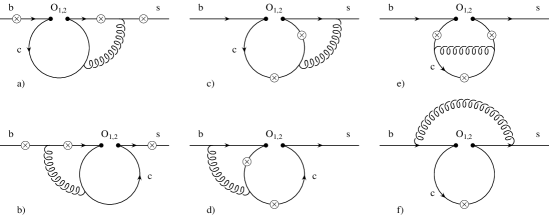
FIG. 1.: Complete list of two-loop Feynman diagrams for $b\rightarrow s\gamma^{*}$ associated with the operators $O_{1}$ and $O_{2}$. The fermions ($b$, $s$ and $c$ quarks) are represented by solid lines; the curly lines represent gluons. The circle-crosses denote the possible locations for emission of a virtual photon.

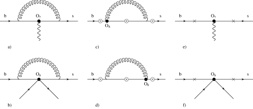
FIG. 2.: Some Feynman diagrams for $b\rightarrow s\gamma^{*}$ or $b\rightarrow s\ell^{+}\ell^{-}$ associated with the operators $O_{7}$, $O_{8}$ and $O_{9}$. The circle-crosses denote the possible locations where the virtual photon is emitted, while the crosses mark the possible locations for gluon bremsstrahlung. See text.

Before we give the result for the renormalized form factors, we remark that only diagram 1f) (and also its renormalized version) suffers from infrared and collinear singularities. As this diagram can easily be combined with diagram 2b) associated with the operator $O_{9}$, we will take it into account in the next subsection, when discussing virtual corrections to $O_{9}$.

We decompose the renormalized matrix elements of $O_{i}$ ($i=1,2$) as

$$\langle s\ell^{+}\ell^{-}|C_{i}^{(0)}O_{i}|b\rangle=C_{i}^{(0)}\left(-\frac{\alpha_{s}}{4\pi}\right)\left[F_{i}^{(9)}\langle\tilde{O}_{9}\rangle_{\text{tree}}+F_{i}^{(7)}\langle\tilde{O}_{7}\rangle_{\text{tree}}\right],$$ (11)

with $\tilde{O}_{9}=\frac{\alpha_{s}}{4\pi}\,O_{9}$ and $\tilde{O}_{7}=\frac{\alpha_{s}}{4\pi}\,O_{7}$. The form factors $F_{i}^{(9)}$ and $F_{i}^{(7)}$ read (using $L_{\mu}=\ln(\mu/m_{b})$, $L_{s}=\ln(\hat{s})$)

$$F_{1}^{(9)} = \left(-{{\frac{1424}{729}}}+{{\frac{16}{243}}}\,i\pi+{{\frac{64}{27}}}\,{L_{c}}\right){L_{\mu}}-{{\frac{16}{243}}}\,{L_{\mu}}\,{L_{s}}+\left({{\frac{16}{1215}}}-{{\frac{32}{135}}}\,{{\hat{m}_{c}}}^{-2}\right){L_{\mu}}\,{\hat{s}}$$ (12)

$$+ \left({{\frac{4}{2835}}}-{{\frac{8}{315}}}\,{{\hat{m}_{c}}}^{-4}\right){L_{\mu}}\,{{\hat{s}}}^{2}+\left({{\frac{16}{76545}}}-{{\frac{32}{8505}}}\,{{\hat{m}_{c}}}^{-6}\right){L_{\mu}}\,{{\hat{s}}}^{3}-{{\frac{256}{243}}}\,{{L_{\mu}}}^{2}+f_{1}^{(9)}\,,$$ (13)

$$F_{2}^{(9)} = \left({{\frac{256}{243}}}-{{\frac{32}{81}}}\,i\pi-{{\frac{128}{9}}}\,{L_{c}}\right){L_{\mu}}+{{\frac{32}{81}}}\,{L_{\mu}}\,{L_{s}}+\left(-{{\frac{32}{405}}}+{{\frac{64}{45}}}\,{{\hat{m}_{c}}}^{-2}\right){L_{\mu}}\,{\hat{s}}$$ (14)

$$+ \left(-{{\frac{8}{945}}}+{{\frac{16}{105}}}\,{{\hat{m}_{c}}}^{-4}\right){L_{\mu}}\,{{\hat{s}}}^{2}+\left(-{{\frac{32}{25515}}}+{{\frac{64}{2835}}}\,{{\hat{m}_{c}}}^{-6}\right){L_{\mu}}\,{{\hat{s}}}^{3}+{{\frac{512}{81}}}\,{{L_{\mu}}}^{2}+f_{2}^{(9)}\,,$$ (15)

$$F_{1}^{(7)}=-{{\frac{208}{243}}}\,{L_{\mu}}+f_{1}^{(7)},\quad\quad F_{2}^{(7)}={{\frac{416}{81}}}\,{L_{\mu}}+f_{2}^{(7)}\,.$$ (16)

The analytic results for $f_{1}^{(9)}$, $f_{1}^{(7)}$, $f_{2}^{(9)}$, and $f_{2}^{(7)}$ (expanded up to $\hat{s}^{3}$ and $(\hat{m}_{c}^{2})^{3}$) are rather lengthy. The formulas become relatively short, however, if we give the charm quark mass dependence in numerical form (for the characteristic values of $\hat{m}_{c}$=0.27, 0.29 and 0.31). We write the functions $f_{a}^{(b)}$ as

$$f_{a}^{(b)}=\sum_{i,j}\,k_{a}^{(b)}(i,j)\,\hat{s}^{i}\,L_{s}^{j}\quad\quad\quad(a=1,2;\,b=7,9;\,i=0,...,3;\,j=0,1).$$ (17)

The numerical values for the quantities $k_{a}^{(b)}(i,j)$ are given in Tab. I and II.

	$\hat{m}_{c}=0.27$			$\hat{m}_{c}=0.29$			$\hat{m}_{c}=0.31$
$k_{1}^{(9)}(0,0)$	$-12.327$	$+$	$0.13512\,i$	$-11.973$	$+$	$0.16371\,i$	$-11.65$	$+$	$0.18223\,i$
$k_{1}^{(9)}(0,1)$	$-0.080505$	$-$	$0.067181\,i$	$-0.081271$	$-$	$0.059691\,i$	$-0.080959$	$-$	$0.051864\,i$
$k_{1}^{(9)}(1,0)$	$-33.015$	$-$	$0.42492\,i$	$-28.432$	$-$	$0.25044\,i$	$-24.709$	$-$	$0.13474\,i$
$k_{1}^{(9)}(1,1)$	$-0.041008$	$+$	$0.0078685\,i$	$-0.040243$	$+$	$0.016442\,i$	$-0.036585$	$+$	$0.024753\,i$
$k_{1}^{(9)}(2,0)$	$-76.2$	$-$	$1.5067\,i$	$-57.114$	$-$	$0.86486\,i$	$-43.588$	$-$	$0.4738\,i$
$k_{1}^{(9)}(2,1)$	$-0.042685$	$+$	$0.015754\,i$	$-0.035191$	$+$	$0.027909\,i$	$-0.021692$	$+$	$0.036925\,i$
$k_{1}^{(9)}(3,0)$	$-197.81$	$-$	$4.6389\,i$	$-128.8$	$-$	$2.5243\,i$	$-86.22$	$-$	$1.3542\,i$
$k_{1}^{(9)}(3,1)$	$-0.039021$	$+$	$0.039384\,i$	$-0.017587$	$+$	$0.050639\,i$	$0.013282$	$+$	$0.052023\,i$
$k_{1}^{(7)}(0,0)$	$-0.72461$	$-$	$0.093424\,i$	$-0.68192$	$-$	$0.074998\,i$	$-0.63944$	$-$	$0.05885\,i$
$k_{1}^{(7)}(0,1)$		0			0			0
$k_{1}^{(7)}(1,0)$	$-0.26156$	$-$	$0.15008\,i$	$-0.23935$	$-$	$0.12289\,i$	$-0.21829$	$-$	$0.10031\,i$
$k_{1}^{(7)}(1,1)$	$-0.00017705$	$+$	$0.02054\,i$	$0.0027424$	$+$	$0.019676\,i$	$0.0053227$	$+$	$0.018302\,i$
$k_{1}^{(7)}(2,0)$	$0.023851$	$-$	$0.20313\,i$	$-0.0018555$	$-$	$0.175\,i$	$-0.022511$	$-$	$0.14836\,i$
$k_{1}^{(7)}(2,1)$	$0.020327$	$+$	$0.016606\,i$	$0.022864$	$+$	$0.011456\,i$	$0.023615$	$+$	$0.0059255\,i$
$k_{1}^{(7)}(3,0)$	$0.42898$	$-$	$0.099202\,i$	$0.28248$	$-$	$0.12783\,i$	$0.17118$	$-$	$0.12861\,i$
$k_{1}^{(7)}(3,1)$	$0.031506$	$+$	$0.00042591\,i$	$0.029027$	$-$	$0.0082265\,i$	$0.022653$	$-$	$0.0155\,i$

TABLE I.: Coefficients in the decomposition of $f_{1}^{(9)}$ and $f_{1}^{(7)}$ for three values of $\hat{m}_{c}$ (eq. (17)).

	$\hat{m}_{c}=0.27$			$\hat{m}_{c}=0.29$			$\hat{m}_{c}=0.31$
$k_{2}^{(9)}(0,0)$	$7.9938$	$-$	$0.81071\,i$	$6.6338$	$-$	$0.98225\,i$	$5.4082$	$-$	$1.0934\,i$
$k_{2}^{(9)}(0,1)$	$0.48303$	$+$	$0.40309\,i$	$0.48763$	$+$	$0.35815\,i$	$0.48576$	$+$	$0.31119\,i$
$k_{2}^{(9)}(1,0)$	$5.1651$	$+$	$2.5495\,i$	$3.3585$	$+$	$1.5026\,i$	$1.9061$	$+$	$0.80843\,i$
$k_{2}^{(9)}(1,1)$	$0.24605$	$-$	$0.047211\,i$	$0.24146$	$-$	$0.098649\,i$	$0.21951$	$-$	$0.14852\,i$
$k_{2}^{(9)}(2,0)$	$-0.45653$	$+$	$9.0402\,i$	$-1.1906$	$+$	$5.1892\,i$	$-1.8286$	$+$	$2.8428\,i$
$k_{2}^{(9)}(2,1)$	$0.25611$	$-$	$0.094525\,i$	$0.21115$	$-$	$0.16745\,i$	$0.13015$	$-$	$0.22155\,i$
$k_{2}^{(9)}(3,0)$	$-25.981$	$+$	$27.833\,i$	$-17.12$	$+$	$15.146\,i$	$-12.113$	$+$	$8.1251\,i$
$k_{2}^{(9)}(3,1)$	$0.23413$	$-$	$0.2363\,i$	$0.10552$	$-$	$0.30383\,i$	$-0.079692$	$-$	$0.31214\,i$
$k_{2}^{(7)}(0,0)$	$4.3477$	$+$	$0.56054\,i$	$4.0915$	$+$	$0.44999\,i$	$3.8367$	$+$	$0.3531\,i$
$k_{2}^{(7)}(0,1)$		0			0			0
$k_{2}^{(7)}(1,0)$	$1.5694$	$+$	$0.9005\,i$	$1.4361$	$+$	$0.73732\,i$	$1.3098$	$+$	$0.60185\,i$
$k_{2}^{(7)}(1,1)$	$0.0010623$	$-$	$0.12324\,i$	$-0.016454$	$-$	$0.11806\,i$	$-0.031936$	$-$	$0.10981\,i$
$k_{2}^{(7)}(2,0)$	$-0.14311$	$+$	$1.2188\,i$	$0.011133$	$+$	$1.05\,i$	$0.13507$	$+$	$0.89014\,i$
$k_{2}^{(7)}(2,1)$	$-0.12196$	$-$	$0.099636\,i$	$-0.13718$	$-$	$0.068733\,i$	$-0.14169$	$-$	$0.035553\,i$
$k_{2}^{(7)}(3,0)$	$-2.5739$	$+$	$0.59521\,i$	$-1.6949$	$+$	$0.76698\,i$	$-1.0271$	$+$	$0.77168\,i$
$k_{2}^{(7)}(3,1)$	$-0.18904$	$-$	$0.0025554\,i$	$-0.17416$	$+$	$0.049359\,i$	$-0.13592$	$+$	$0.093\,i$

TABLE II.: Coefficients in the decomposition of $f_{2}^{(9)}$ and $f_{2}^{(7)}$ for three values of $\hat{m}_{c}$ (eq. (17)).

B Virtual corrections to the matrix elements of $O_{7}$, $O_{8}$ and $O_{9}$

We first turn to the virtual corrections to the matrix element of the operator $O_{9}$, consisting of the vertex correction shown in Fig. 2b) and of the quark self-energy contributions. The sum of these corrections is ultraviolet finite, but suffers from infrared and collinear singularities. The result can be written as

$$\langle s\ell^{+}\ell^{-}|C_{9}O_{9}|b\rangle=\tilde{C}_{9}^{(0)}\left(-\frac{\alpha_{s}}{4\pi}\right)\left[F_{9}^{(9)}\langle\tilde{O}_{9}\rangle_{\text{tree}}+F_{9}^{(7)}\langle\tilde{O}_{7}\rangle_{\text{tree}}\right],$$ (18)

with $\tilde{O}_{9}=\frac{\alpha_{s}}{4\pi}\,O_{9}$ and $\tilde{C}_{9}^{(0)}=\frac{4\pi}{\alpha_{s}}\left(C_{9}^{(0)}+\frac{\alpha_{s}}{4\pi}C_{9}^{(1)}\right)$. The form factors $F_{9}^{(9)}$ and $F_{9}^{(7)}$ read (keeping terms up to order $\hat{s}^{3}$)

$$F_{9}^{(9)}={\frac{16}{3}}+{\frac{20}{3}}\hat{s}+{\frac{16}{3}}\hat{s}^{2}+{\frac{116}{27}}\hat{s}^{3}+f_{\rm{inf}}\,,$$ (19)

$$F_{9}^{(7)}=-{\frac{2}{3}}\hat{s}\left(1+{\frac{1}{2}}\hat{s}+{\frac{1}{3}}\hat{s}^{2}\right)\,,$$ (20)

where the function $f_{\rm{inf}}$ contains the infrared and collinear singularities. Its explicit form is (using $r=(m_{s}/m_{b})^{2}$)

$$f_{\rm{inf}}=\frac{\left(\frac{\mu}{m_{b}}\right)^{2\epsilon}}{\epsilon}\,\frac{8}{3}\,(1+\hat{s}+\frac{1}{2}\hat{s}^{2}+\frac{1}{3}\hat{s}^{3})+\frac{4}{3}\frac{\left(\frac{\mu}{m_{b}}\right)^{2\epsilon}}{\epsilon}\,\ln r+\frac{2}{3}\ln r-\frac{2}{3}\ln^{2}r\,.$$ (21)

At this place, it is convenient to incorporate the renormalized diagram 1f), which has not been taken into account so far. It is easy to see that the two loops factorize into two one-loop contributions. The charm loop has the Lorentz structure of $O_{9}$ and can therefore be absorbed into an effective Wilson coefficient: Diagram 1f) is properly included by modifying $\tilde{C}^{(0)}_{9}$ in eq. (18) as follows:

$$\tilde{C}^{(0)}_{9}\longrightarrow\tilde{C}^{(0,\text{mod})}_{9}=\tilde{C}^{(0)}_{9}+\left(C_{2}^{(0)}+\frac{4}{3}C_{1}^{(0)}\right)\,H_{0}\,,$$ (22)

where the charm-loop function $H_{0}$ reads (in expanded form)

$$H_{0}=\frac{1}{2835}\left[-1260+2520\ln(\mu/m_{c})+252\hat{s}\hat{m}_{c}^{-2}+27\hat{s}^{2}\hat{m}_{c}^{-4}+4\hat{s}^{3}\hat{m}_{c}^{-6}\right]\,.$$ (23)

In the context of virtual corrections also the $O(\epsilon)$-part of this loop function is needed. We neglect it here since it will drop out in combination with gluon bremsstrahlung. Note that $H_{0}=h(\hat{m}_{c}^{2},\hat{s})+8/9\,\ln(\mu/m_{b})$, with $h$ defined in [12, 13].

We now turn to the virtual corrections to the matrix element of the operator $O_{7}$, consisting of the vertex- (Fig. 2a) and self-energy corrections. The sum of these diagrams is ultraviolet singular. After renormalization, the result can be written as

$$\langle s\ell^{+}\ell^{-}|C_{7}O_{7}|b\rangle=\tilde{C}_{7}^{(0)}\left(-\frac{\alpha_{s}}{4\pi}\right)\left[F_{7}^{(9)}\langle\tilde{O}_{9}\rangle_{\text{tree}}+F_{7}^{(7)}\langle\tilde{O}_{7}\rangle_{\text{tree}}\right],$$ (24)

with $\tilde{O}_{7}=\frac{\alpha_{s}}{4\pi}\,O_{7}$ and $\tilde{C}_{7}^{(0)}=C_{7}^{(1)}$. The form factors $F_{7}^{(9)}$ and $F_{7}^{(7)}$ read

$$F_{7}^{(9)}=-{\frac{16}{3}}\left(1+{\frac{1}{2}}\hat{s}+{\frac{1}{3}}\hat{s}^{2}+{\frac{1}{4}}\hat{s}^{3}\right)\,,$$ (25)

$$F_{7}^{(7)}={{\frac{32}{3}}}\,{L_{\mu}}+{\frac{32}{3}}+8\hat{s}+6\hat{s}^{2}+{\frac{128}{27}}\hat{s}^{3}+f_{\rm{inf}}\,.$$ (26)

Note that for these expressions the pole mass for $m_{b}$ has to be used at lowest order.

Finally, we give the result for the renormalized corrections to the matrix elements of $O_{8}$. The corresponding diagrams are shown in Fig. 2c) and 2d). One obtains:

$$\langle s\ell^{+}\ell^{-}|C_{8}O_{8}|b\rangle=\tilde{C}_{8}^{(0)}\left(-\frac{\alpha_{s}}{4\pi}\right)\left[F_{8}^{(9)}\langle\tilde{O}_{9}\rangle_{\text{tree}}+F_{8}^{(7)}\langle\tilde{O}_{7}\rangle_{\text{tree}}\right],$$ (27)

with $\tilde{C}_{8}^{(0)}=C_{8}^{(1)}$. The form factors $F_{8}^{(9)}$ and $F_{8}^{(7)}$ read (in expanded form)

$$F_{8}^{(9)} = {\frac{104}{9}}-{\frac{32}{27}}\pi^{2}+\left({\frac{1184}{27}}-{\frac{40}{9}}\pi^{2}\right)\hat{s}+\left({\frac{14212}{135}}-{\frac{32}{3}}\pi^{2}\right)\hat{s}^{2}$$ (28)

$$+ \left({\frac{193444}{945}}-{\frac{560}{27}}\pi^{2}\right)\hat{s}^{3}+{\frac{16}{9}}L_{s}\left(1+\hat{s}+\hat{s}^{2}+\hat{s}^{3}\right)\,,$$ (29)

$$F_{8}^{(7)} = -{\frac{32}{9}}\,L_{\mu}+{\frac{8}{27}}\pi^{2}-{\frac{44}{9}}-{\frac{8}{9}}i\pi+\left({\frac{4}{3}}\pi^{2}-{\frac{40}{3}}\right)\hat{s}+\left({\frac{32}{9}}\pi^{2}-{\frac{316}{9}}\right)\hat{s}^{2}$$ (30)

$$+ \left({\frac{200}{27}}\pi^{2}-{\frac{658}{9}}\right)\hat{s}^{3}-{\frac{8}{9}}\,L_{s}\left(\hat{s}+\hat{s}^{2}+\hat{s}^{3}\right)\,.$$ (31)

IV Bremsstrahlung corrections

We stress that in the present paper only those bremsstrahlung diagrams are taken into account which are needed to cancel the infrared and collinear singularities from the virtual corrections. All other bremsstrahlung contributions (which are finite), will be given elsewhere [20].

It is known [11, 12] that the contribution to the inclusive decay width coming from the interference between the tree-level and the one-loop matrix elements of $O_{9}$ (Fig. 2b)) and from the corresponding bremsstrahlung corrections (Fig. 2f)), can be written in the form

$$\frac{d\Gamma_{99}}{d\hat{s}}=\left(\frac{\alpha_{em}}{4\pi}\right)^{2}\frac{G_{F}^{2}m_{b,pole}^{5}\left|V_{ts}^{*}V_{tb}\right|^{2}}{48\pi^{3}}(1-\hat{s})^{2}\left(1+2\hat{s}\right)\left(2\left(\widetilde{C}_{9}^{(0)}\right)^{2}\frac{\alpha_{s}}{\pi}\omega_{9}(\hat{s})\right),$$ (32)

where $\widetilde{C}_{9}^{(0)}=\frac{4\pi}{\alpha_{s}}\left(C_{9}^{(0)}+\frac{\alpha_{s}}{4\pi}C_{9}^{(1)}\right)$; the function $\omega_{9}(\hat{s})\equiv\omega(\hat{s})$, which contains information on virtual and bremsstrahlung corrections, can be found in [11, 12]. Replacing $\tilde{C}_{9}^{(0)}$ by $\tilde{C}_{9}^{(0,\text{mod})}$ (see eq. (22)) in eq. (32), diagram 1f) and the corresponding bremsstrahlung corrections are automatically included.

Similarly, the contribution to the decay width from the interference between the tree-level and the one-loop matrix element of $O_{7}$ (Fig. 2a), combined with the corresponding bremsstrahlung corrections shown in Fig. 2e), can be written as

$$\frac{d\Gamma_{77}}{d\hat{s}}=\left(\frac{\alpha_{em}}{4\pi}\right)^{2}\frac{G_{F}^{2}m_{b,pole}^{5}\left|V_{ts}^{*}V_{tb}\right|^{2}}{48\pi^{3}}(1-\hat{s})^{2}4\left(1+2/\hat{s}\right)\left(2\left(\widetilde{C}_{7}^{(0)}\right)^{2}\frac{\alpha_{s}}{\pi}\omega_{7}(\hat{s})\right),$$ (33)

where $\widetilde{C}_{7}^{(0)}=C_{7}^{(1)}$. The function $\omega_{7}(\hat{s})$, which is new, reads

$$\omega_{7}(\hat{s}) = -\frac{8}{3}\,\ln\left(\frac{\mu}{m_{b}}\right)-\frac{4}{3}\,\mbox{Li}(\hat{s})-\frac{2}{9}\,{\pi}^{2}-\frac{2}{3}\,\ln(\hat{s})\ln(1-\hat{s})$$ (35)

$$-\frac{1}{3}\,\frac{8+\hat{s}}{2+\hat{s}}\ln(1-\hat{s})-\frac{2}{3}\,\frac{\hat{s}\left(2-2\,\hat{s}-\hat{s}^{2}\right)}{\left(1-\hat{s}\right)^{2}\left(2+\hat{s}\right)}\ln(\hat{s})-\frac{1}{18}\,\frac{16-11\,\hat{s}-17\,\hat{s}^{2}}{\left(2+\hat{s}\right)\left(1-\hat{s}\right)}\,.$$

Finally, one observes that also the interference between the tree-level matrix element of $O_{7}$ and the one-loop matrix element of $O_{9}$ (and vice versa) lead to an infrared singular contribution to the decay width. We combined it with the corresponding bremsstrahlung terms coming from the interference of diagrams 2e) and 2f). The result reads

$$\frac{d\Gamma_{79}}{d\hat{s}}=\left(\frac{\alpha_{em}}{4\pi}\right)^{2}\frac{G_{F}^{2}m_{b,pole}^{5}\left|V_{ts}^{*}V_{tb}\right|^{2}}{48\pi^{3}}(1-\hat{s})^{2}12\cdot 2\frac{\alpha_{s}}{\pi}\omega_{79}(\hat{s})\mbox{Re}\left(\widetilde{C}_{7}^{(0)}\widetilde{C}_{9}^{(0)}\right)\,.$$ (36)

For the function $\omega_{79}(\hat{s})$, which also is new, we obtain

$$\omega_{79}(\hat{s}) = -\frac{4}{3}\,\ln\left(\frac{\mu}{m_{b}}\right)-\frac{4}{3}\,\mbox{Li}(\hat{s})-\frac{2}{9}\,{\pi}^{2}-\frac{2}{3}\,\ln(\hat{s})\ln(1-\hat{s})$$ (38)

$$-\frac{1}{9}\,\frac{2+7\hat{s}}{\hat{s}}\ln(1-\hat{s})-\frac{2}{9}\,\frac{\hat{s}\left(3-2\,\hat{s}\right)}{\left(1-\hat{s}\right)^{2}}\ln(\hat{s})+\frac{1}{18}\,\frac{5-9\,\hat{s}}{1-\hat{s}}\,.$$

V Corrections to the decay width for $b\rightarrow X_{s}\ell^{+}\ell^{-}$

In this section we combine the virtual corrections calculated in section III and the bremsstrahlung contributions discussed in section IV and study their influence on the decay width $d\Gamma(b\rightarrow X_{s}\ell^{+}\ell^{-})/d\hat{s}$. In the literature (see e.g. [13]), this decay width is usually written as

$$\frac{d\Gamma(b\rightarrow X_{s}\ell^{+}\ell^{-})}{d\hat{s}}=\left(\frac{\alpha_{em}}{4\pi}\right)^{2}\frac{G_{F}^{2}m_{b,pole}^{5}\left|V_{ts}^{*}V_{tb}\right|^{2}}{48\pi^{3}}(1-\hat{s})^{2}\times$$ (39)

$$\left(\left(1+2\hat{s}\right)\left(\left|\widetilde{C}_{9}^{\text{eff}}\right|^{2}+\left|\widetilde{C}_{10}^{\text{eff}}\right|^{2}\right)+4\left(1+2/\hat{s}\right)\left|\widetilde{C}_{7}^{\text{eff}}\right|^{2}+12\mbox{Re}\left(\widetilde{C}_{7}^{\text{eff}}\widetilde{C}_{9}^{\text{eff}*}\right)\right)\,,$$ (40)

where the contributions calculated so far have been absorbed into the effective Wilson coefficients $\tilde{C}_{7}^{\text{eff}}$, $\tilde{C}_{9}^{\text{eff}}$ and $\tilde{C}_{10}^{\text{eff}}$. It turns out that also the new contributions calculated in the present paper can be absorbed into these coefficients. Following as closely as possible the ’parametrization’ given recently by Bobeth et al. [13], we write

$$\widetilde{C}_{9}^{\text{eff}} = \left(1+\frac{\alpha_{s}(\mu)}{\pi}\omega_{9}(\hat{s})\right)\left(A_{9}+T_{9}\,h(\hat{m}_{c}^{2},\hat{s})+U_{9}\,h(1,\hat{s})+W_{9}\,h(0,\hat{s})\right)$$ (42)

$$-\frac{\alpha_{s}(\mu)}{4\pi}\left(C_{1}^{(0)}F_{1}^{(9)}+C_{2}^{(0)}F_{2}^{(9)}+A_{8}^{(0)}F_{8}^{(9)}\right)$$

$$\widetilde{C}_{7}^{\text{eff}} = \left(1+\frac{\alpha_{s}(\mu)}{\pi}\omega_{7}(\hat{s})\right)A_{7}-\frac{\alpha_{s}(\mu)}{4\pi}\left(C_{1}^{(0)}F_{1}^{(7)}+C_{2}^{(0)}F_{2}^{(7)}+A_{8}^{(0)}F_{8}^{(7)}\right)$$ (43)

$$\widetilde{C}_{10}^{\text{eff}} = \left(1+\frac{\alpha_{s}(\mu)}{\pi}\omega_{9}(\hat{s})\right)A_{10}\,,$$ (44)

where the expressions for $h(\hat{m}_{c}^{2},\hat{s})$ and $\omega_{9}(\hat{s})$ are given in [13]. The quantities $\omega_{7}(\hat{s})$ and $F_{1,2,8}^{(7,9)}$, on the other hand, have been calculated in the present paper. We take the numerical values for $A_{7}$, $A_{9}$, $A_{10}$, $T_{9}$, $U_{9}$, and $W_{9}$ from [13], while $C_{1}^{(0)}$, $C_{2}^{(0)}$ and $A_{8}^{(0)}=\tilde{C}_{8}^{(0,\text{eff})}$ are taken from [19]. For completeness we list them in Tab. III.

	$\mu=2.5$ GeV	$\mu=5$ GeV	$\mu=10$ GeV
$\alpha_{s}$	$0.267$	$0.215$	$0.180$
$C_{1}^{(0)}$	$-0.697$	$-0.487$	$-0.326$
$C_{2}^{(0)}$	$1.046$	$1.024$	$1.011$
$(A_{7}^{(0)},A_{7}^{(1)})$	$(-0.360,0.031)$	$(-0.321,0.019)$	$(-0.287,0.008)$
$A_{8}^{(0)}$	$-0.164$	$-0.148$	$-0.134$
$(A_{9}^{(0)},A_{9}^{(1)})$	$(4.241,-0.170)$	$(4.129,0.013)$	$(4.131,0.155)$
$(T_{9}^{((0))},T_{9}^{(1)})$	$(0.115,0.278)$	$(0.374,0.251)$	$(0.576,0.231)$
$(U_{9}^{(0)},U_{9}^{(1)})$	$(0.045,0.023)$	$(0.032,0.016)$	$(0.022,0.011)$
$(W_{9}^{(0)},W_{9}^{(1)})$	$(0.044,0.016)$	$(0.032,0.012)$	$(0.022,0.009)$
$(A_{10}^{(0)},A_{10}^{(1)})$	$(-4.372,0.135)$	$(-4.372,0.135)$	$(-4.372,0.135)$

TABLE III.: Coefficients appearing in eq. (42) for $\mu=2.5$ GeV, $\mu=5$ GeV and $\mu=10$ GeV. For $\alpha_{s}(\mu)$ (in the $\overline{\mbox{MS}}$ scheme) we used the two-loop expression with 5 flavors and $\alpha_{s}(m_{Z})=0.119$. The entries correspond to the pole top quark mass $m_{t}=174$ GeV. The superscript $(0)$ refers to lowest order quantities and while the superscript $(1)$ denotes the correction terms of order $\alpha_{s}$.

When calculating the decay width (39), we retain only terms linear in $\alpha_{s}$ (and thus in $\omega_{9}$ and $\omega_{7}$) in $|\widetilde{C}_{9}^{\text{eff}}|^{2}$ and $|\widetilde{C}_{7}^{\text{eff}}|^{2}$. In the interference term $\mbox{Re}\left(\widetilde{C}_{7}^{\text{eff}}\widetilde{C}_{9}^{\text{eff}*}\right)$ too, we keep only terms linear in $\alpha_{s}$. By construction, one has to make the replacements $\omega_{9}\rightarrow\omega_{79}$ and $\omega_{7}\rightarrow\omega_{79}$ in this term.

Our results include all the relevant virtual corrections and singular bremsstrahlung contributions. There exist additional bremsstrahlung terms coming e.g. from one-loop $O_{1}$ and $O_{2}$ diagrams in which both, the virtual photon and the gluon are emitted from the charm quark line. These contributions do not induce additional renormalization scale dependence as they are ultraviolet finite. Using our experience from $b\rightarrow s\gamma$ and $b\rightarrow sg$, these contributions are not expected to be large.

VI Numerical results

The decay width in eq. (39) has a large uncertainty due to the factor $m_{b,pole}^{5}$. Following common practice, we consider the ratio

$$R_{\text{quark}}(\hat{s})=\frac{1}{\Gamma(b\rightarrow X_{c}e\bar{\nu})}\frac{d\Gamma(b\rightarrow X_{s}\ell^{+}\ell^{-})}{d\hat{s}}\,,$$ (45)

in which the factor $m_{b,pole}^{5}$ drops out. The explicit expression for the semi-leptonic decay width $\Gamma(b\rightarrow X_{c}e\nu_{e})$ can be found e.g. in [13].

We now turn to the numerical results for $R_{\text{quark}}(\hat{s})$ for $0.05\leq\hat{s}\leq 0.25$. In Fig. 3a we investigate the dependence of $R_{\text{quark}}(\hat{s})$ on the renormalization scale $\mu$. The solid lines are obtained by including the new NNLL contributions as explained in detail in section V. The three solid lines correspond to $\mu=2.5$ GeV (lower line), $\mu=5$ GeV (middle line) and $\mu=10$ GeV (upper line). The three dashed lines (again $\mu=2.5$ GeV for the lower, $\mu=5$ GeV for the middle and $\mu=10$ GeV for the upper curve), on the other hand, show the results without the new NNLL corrections, i.e., they include the NLL results combined with the NNLL corrections to the matching conditions as obtained by Bobeth et al. [13]. From this figure we conclude that the renormalization scale dependence gets reduced by more than a factor of 2. Only for small values of $\hat{s}$ ($\hat{s}\sim 0.05$), where the NLL $\mu$-dependence is small already, the reduction factor is smaller. For the integrated quantity we obtain

$$R_{\text{quark}}=\int_{0.05}^{0.25}\,d\hat{s}\,R_{\text{quark}}(\hat{s})=(1.25\pm 0.08)\times 10^{-5}\,,$$ (46)

where the error is obtained by varying $\mu$ between 2.5 GeV and 10 GeV. Before our corrections, the result was $R_{\text{quark}}=(1.36\pm 0.18)\times 10^{-5}$ [13]. In other words, the renormalization scale dependence got reduced from $\sim\pm 13\%$ to $\sim\pm 6.5\%$.

Among the errors on $R_{\text{quark}}(\hat{s})$ which are due to the uncertainties in the input parameters, the one induced by $\hat{m}_{c}=m_{c}/m_{b}$ is known to be the largest. We therefore show in Fig. 3b the dependence of $R_{\text{quark}}(\hat{s})$ on $\hat{m}_{c}$. Comparing Fig. 3a with Fig. 3b, we find that the uncertainty due to $\hat{m}_{c}$ is somewhat larger than the left-over $\mu$-dependence at the NNLL level. For the integrated quantity $R_{\text{quark}}$ we find an uncertainty of $\pm 7.6\%$ due to $\hat{m}_{c}$.

To conclude: We have calculated virtual corrections of order $\alpha_{s}$ to the matrix elements of $O_{1}$, $O_{2}$, $O_{7}$, $O_{8}$, $O_{9}$ and $O_{10}$. We also took into account those bremsstrahlung corrections which cancel the infrared and collinear singularities in the virtual corrections. The renormalization scale dependence of $R_{\text{quark}}(\hat{s})$ gets reduced by more than a factor of 2. The calculation of the remaining bremsstrahlung contributions (which are expected to be rather small) and a more detailed numerical analysis are in progress [20].

FIG. 3.: (a) The three solid lines show the $\mu$ dependence of $R_{\text{quark}}(\hat{s})$ when including the corrections to the matrix elements calculated in this paper; the dashed lines are obtained when switching off these corrections. We set $\hat{m}_{c}=0.29$. (b) $R_{\text{quark}}(\hat{s})$ for $\hat{m}_{c}=0.27$ (dashed line), $\hat{m}_{c}=0.29$ (solid line) and $\hat{m}_{c}=0.31$ (dash-dotted line) and $\mu$=5 GeV. See text.

REFERENCES

- [1] R. Ammar et al. (CLEO Collaboration), Phys. Rev. Lett. 71, 674 (1993).
- [2] R. Ammar et al. (CLEO Collaboration), Phys. Rev. Lett. 74, 2885 (1995).
- [3] S. Glenn et al. (CLEO Collaboration), Phys. Rev. Lett. 80, 2289 (1998).
- [4] Z. Ligeti and M. B. Wise, Phys. Rev. D 53, 4937 (1996).
- [5] A. F. Falk, M. Luke and M. J. Savage, Phys. Rev. D 49, 3367 (1994).
- [6] A. Ali, G. Hiller, L. T. Handoko and T. Morozumi, Phys. Rev. D 55, 4105 (1997) [hep-ph/9609449].
- [7] J-W. Chen, G. Rupak and M. J. Savage, Phys. Lett. B 410, 285 (1997).
- [8] G. Buchalla, G. Isidori and S. J. Rey, Nucl. Phys. B 511, 594 (1998) [hep-ph/9705253].
- [9] G. Buchalla and G. Isidori, Nucl. Phys. B 525, 333 (1998).
- [10] F. Krüger and L.M. Sehgal, Phys. Lett. B 380, 199 (1996).
-
[11]
M. Misiak,
Nucl. Phys. B 393, 23 (1993);
Nucl. Phys. B 439, 461 (1995) (E). - [12] A. J. Buras and M. Münz, Phys. Rev. D 52, 186 (1995) [hep-ph/9501281].
- [13] C. Bobeth, M. Misiak and J. Urban, Nucl. Phys. B 574, 291 (2000) [hep-ph/9910220].
- [14] K. Chetyrkin, M. Misiak and M. Münz, Phys. Lett. B 400, 206 (1997); Nucl. Phys. B 518, 473 (1998); Nucl. Phys. B 520, 279 (1998).
-
[15]
K. Adel and Y. P. Yao,
Phys. Rev. D 49, 4945 (1994);
C. Greub and T. Hurth Phys. Rev. D 56, 2934 (1997);
A. J. Buras, A. Kwiatkowski and N. Pott, Nucl. Phys. B 517, 353 (1998);
M. Ciuchini, G. Degrassi, P. Gambino and G. F. Giudice, Nucl. Phys. B 527, 21 (1998). - [16] G. Buchalla and A. J. Buras, Nucl. Phys. B 548, 309 (1999) [hep-ph/9901288].
- [17] B. Grinstein, M. J. Savage and M. B. Wise, Nucl. Phys. B 319, 271 (1989).
- [18] C. Greub, T. Hurth and D. Wyler, Phys. Rev. D 54, 3350 (1996) [hep-ph/9603404].
- [19] C. Greub and P. Liniger, Phys. Lett. B 494, 237 (2000) [hep-ph/0008071]; Phys. Rev. D 63, 054025 (2001) [hep-ph/0009144].
- [20] H. H. Asatryan, H. M. Asatrian, C. Greub and M. Walker, in preparation.
-
[21]
V.A. Smirnov, hep-th/9412063;
V.A. Smirnov, Renormalization and Asymptotic Expansions, Birkhäuser, Basel, 1991.