We discuss limits on neutrino-Majoron couplings both from laboratory experiments as well as from astrophysics. They apply to the simplest class of Majoron models which covers a variety of possibilities where neutrinos acquire mass either via a seesaw-type scheme or via radiative corrections. By adopting a general framework including CP phases we generalize bounds obtained previously. The combination of complementary bounds enables us to obtain a highly non-trivial exclusion region in the parameter space. We find that the future double beta project GENIUS, together with constraints based on supernova energy release arguments, could restrict neutrino-Majoron couplings down to the $10^{-7}$ level.

1 Introduction

The confirmation of the zenith–angle–dependent atmospheric neutrino deficit by the Superkamiokande experiment generally has been understood as first significant hint for neutrino masses and thus particle physics beyond the standard model [1]. The other long-standing puzzle of particle physics is the deficit of solar neutrinos [2]. Altogether they constitute the most important milestone in the search for phenomena beyond the Standard Model (SM), indicating the need for oscillations involving all three active neutrino species [3]. The mounting experimental activity in this field promises a bright future for neutrino physics which may prove to be a most valuable source of information on the structure of a more complete theory underlying the standard model of particle physics.

An elegant way to introduce neutrino masses is via the spontaneous breaking of an ungauged lepton number symmetry through a non-zero $SU(2)\otimes U(1)$ singlet vacuum expectation value (VEV) of a scalar field. This may be implemented in conventional [4, 5] as well as supersymmetric models  [6]. The couplings of the corresponding Goldstone boson, generically called Majoron and denoted by $J$, are rather model-dependent [7]. Here we consider the simplest class of Majoron models, where the Majoron-neutrino coupling matrix $g_{ij}^{M}\propto m_{ij}$ is proportional to the neutrino mass matrix [8], so that in the mass eigenstate basis diag $(m_{1},m_{2},m_{3})$ the Majoron neutrino couplings $g_{i}$ are diagonal, to lowest order approximation  ,

$$g_{ij}^{M}\simeq\delta_{ij}g_{i}.$$ (1)

This covers a variety of possibilities including both seesaw-type [4] as well as radiative models [5].

Limits on this quantity obtained from laboratory experiments searching for Majoron-emitting pion or kaon decays are rather weak, with the exception of double beta decay [11]. On the other hand Majoron emitting neutrino decays affect the expected neutrino luminosity and spectra which are constrained by the observed signal from SN1987A, providing stringent restrictions [12]. While the limits of laboratory experiments on rare decays are given in the weak basis, bounds from processes in supernovae occur in a dense medium and are expressed in the medium eigenstates (see below). In the present work we discuss the correlations of the different limits and their translation into the mass basis, extending the earlier paper ref. [12]. In the next section we derive the expressions for medium and weak eigenstates, following [12, 13]. In section 3 we review the bounds obtained from the supernova SN1987A using various considerations. In contrast to ref. [12] here we include the study of the effects associated to the Majorana CP violating phases present in theories of massive neutrinos [14, 15]. Moreover we investigate (Section 4) the recent bounds from neutrinoless double beta decay as well as those that could be attained in future experiments such as GENIUS [16]. The resulting exclusion plots are discussed in section 5 in the mass basis.

2 Neutrino mixing in three bases

For neutrinos propagating through a medium one has to deal with three kinds of eigenstates: Flavor eigenstates $\nu_{\alpha}$, mass eigenstates $\nu_{i}^{(h_{i})}$ with masses $m_{i}$, and, depending on the environment, medium eigenstates $\tilde{\nu}_{i}^{(h_{i})}$. The flavor eigenstates are defined as

$$\nu_{\alpha}=\sum_{i}U_{\alpha i}\nu_{i}^{(h_{i})}$$ (2)

and the medium eigenstates are

$$\tilde{\nu}^{(h_{i})}_{i}=\sum_{j}\tilde{U}_{ij}\nu_{j}^{(h_{j})}.$$ (3)

Here the superscript $(h_{i})=\pm 1$ refers to the helicity of the state. In the general case it is impossible to diagonalize simultaneously the mass and potential terms. Thus one has to solve the field equations in detail. In a two-component field formalism, where a left-handed four-component field $\nu$ expressed in the chiral representation of the $\gamma$ matrices [14] is related to the corresponding two-component field $\phi$ by $\nu_{L}^{T}=(\phi^{T},0)$ [13] , the Lagrangian can be written in the mass basis as

$$\mathcal{L}_{\rm tot} = \mathcal{L}_{\rm 0}+\mathcal{L}_{\rm med}+\mathcal{L}_{\rm int}$$ (4)

$$= \sum_{i}\phi_{i}^{\dagger}(i\partial_{0}-i{\vec{\sigma}}\times{\vec{\nabla}})\phi_{i}-\frac{m_{i}}{2}(\phi_{i}^{T}i\sigma_{2}\phi_{i}-\phi_{i}^{\dagger}i\sigma_{2}\phi^{*})+\sum_{i,j}\phi_{i}^{\dagger}V_{ij}\phi_{j}-$$

$$-J\sum_{ij}g^{M}_{ij}(\phi_{i}^{T}\sigma_{2}\phi_{j}+\phi_{i}^{\dagger}\sigma_{2}\phi_{j}^{*})$$

where $\sigma_{2}$ and $\vec{\sigma}$ denote Pauli matrices. Here the free Langrangian ${\mathcal{L}}_{0}$ and $\mathcal{L}_{\rm med}$ describe the propagation in vacuo and the effects of matter described by the potential matrix $V_{ij}$, respectively, whereas $\mathcal{L}_{\rm int}$ takes into account the presence of neutrino-Majoron interactions which may lead to decays. One has now to consider the decays $\tilde{\nu}_{i}^{h_{i}}\!(p_{i})\to\tilde{\nu}_{j}^{h_{j}}\!(p_{j})+J(q)$, where $\tilde{\nu}_{i}^{h_{i}}\!(p_{i})$ and $\tilde{\nu}_{j}^{h_{j}}\!(p_{j})$ are energy–eigenstate Majorana neutrinos that propagate in matter with four-momenta $p_{i}=(E_{i}^{h_{i}},{\vec{p}_{i}})$ and $p_{j}=(E_{j}^{h_{j}},{\vec{p}_{j}})$, and helicity $h_{i}$ and $h_{f}$ respectively. In order to obtain these energy–eigenstates one has to take $\cal{L}_{\rm{0}}+\cal{L}_{\rm med}$ and calculate the resulting field equations.

$$(i\partial_{0}-i\vec{\sigma}\times\vec{\nabla})\phi_{i}(x)+m_{i}i\sigma_{2}\phi_{i}^{*}-\sum_{j=1}^{N}V_{ij}\phi_{j}(x)=0.$$ (5)

One solves these field equations by expanding the fields $\phi_{i}(x)$ as superpositions of plane-wave spinors with definite helicity, [13, 17],

$$\phi_{i}(x)=\int\frac{d\vec{p}}{\sqrt{(2\pi)^{3}}}e^{i\vec{p}\times\vec{x}}\left\{[P_{\alpha}^{i}(\vec{p},t)+N_{\alpha}^{i}(\vec{p},t)]\alpha(\vec{p})+[P_{\beta}^{i}(\vec{p},t)+N_{\beta}^{i}(\vec{p},t)]\beta(\vec{p})\right\}$$ (6)

where $\alpha(\vec{p})$ and $\beta(\vec{k})$ are helicity eigenstates and $P^{i}$ and $N^{i}$ denote positive and negative frequency components of the field under consideration. One should now substitute this expression in the equations (5), whose diagonalization would give rise to the desired eigenstates. It can be shown, though, that for relativistic neutrinos the positive-frequency components decouple from the negative-frequency ones and the energy eigenstates obtained in this way result to be the same as those obtained from the diagonalization of the usual MSW equation [13], which can be stated as

$$i\partial_{t}\nu_{i}^{(h)}=(H^{\rm rel}_{ij}+U_{i\alpha}V_{\alpha\beta}U^{\dagger}_{\beta j})\nu_{j}^{(h)}.$$ (7)

Here $H^{\rm rel}_{ij}\approx(p+m_{i}^{2}/(2p))\delta_{ij}$ and $V_{\alpha\beta}$ is the potential matrix in the weak basis,

$$V_{\alpha\beta}=\left(\begin{array}[]{ccc}V_{C}+V_{N}&0&0\\ 0&V_{N}&0\\ 0&0&V_{N}\end{array}\right)\,.$$ (8)

The potentials induced by the charged and neutral currents are $V_{C}=\sqrt{2}hG_{F}n_{B}(Y_{e}+Y_{\nu_{e}})$ and $V_{N}=\sqrt{2}hG_{F}n_{B}\left(-\frac{1}{2}Y_{N}+Y_{\nu_{e}}\right)$, where $Y_{i}=(n_{i}-n_{\bar{i}})/n_{B}$ and $n_{B}$ is the baryon density. Diagonalizing $H^{\rm rel}+UVU^{\dagger}$ yields the medium eigenstates $\tilde{\nu}_{i}^{(h)}=\tilde{U}_{ij}^{(h)}\nu_{j}^{(h)}$.

medium state	weak state	potential
$\tilde{\nu}_{1}^{(+)}$	$\bar{\nu}_{e}$	$-(V_{C}+V_{N})$
$\tilde{\nu}_{2}^{(+)}$	$\bar{\nu}_{\mu^{\prime}}=c_{23}\bar{\nu}_{\mu}-s_{23}\bar{\nu}_{\tau}$	$-V_{N}$
$\tilde{\nu}_{3}^{(+)}$	$\bar{\nu}_{\tau^{\prime}}=s_{23}\bar{\nu}_{\mu}+c_{23}\bar{\nu}_{\tau}$	$-V_{N}$
$\tilde{\nu}_{1}^{(-)}$	$\nu_{\mu^{\prime}}=c_{23}\nu_{\mu}-s_{23}\nu_{\tau}$	$V_{N}$
$\tilde{\nu}_{2}^{(-)}$	$\nu_{\tau^{\prime}}=s_{23}\nu_{\mu}+c_{23}\nu_{\tau}$	$V_{N}$
$\tilde{\nu}_{3}^{(-)}$	$\nu_{e}$	$V_{C}+V_{N}$

Table 1: Medium eigenstates $\tilde{\nu}_{i}^{\pm}$, equivalent weak eigenstates in the limit $|V_{\alpha\alpha}|\gg m_{i}^{2}/(2p)$ and their potential energy. The rotation in the $\nu_{\mu}-\nu_{\tau}$ subspace is parametrized by $c_{23}=\cos\theta_{23}$ and $s_{23}=\sin\theta_{23}$, where the arbitrary argument has been chosen to coincide with the mixing angle $\theta_{23}$ in vacuo (from [12]).

In the three-flavor neutrino case the mixing matrix $U$ can be parametrized as $U=U_{23}U_{13}U_{12}U_{0}$, where the matrices $U_{ij}=U_{ij}(\theta_{ij})$ perform the rotation in the $ij$-plane by the angle $\theta_{ij}$ and $U_{0}$ includes possible CP-violation effects [14, 15]. In the following we will assumme $\theta_{13}=0$, motivated both by detailed fits of the present solar and atmospheric neutrino anomalies [3] as well as by the reactor results of the Chooz experiment [18]. This simplifies the mixing matrix to $\nu_{\alpha}=U_{\alpha i}\nu_{i}=U_{23}U_{12}U_{0}\nu_{i}$ [19] and allows us to set $\theta_{12}=\theta_{\odot}$ and $\theta_{23}=\theta_{\rm atm}$. Now for light neutrinos near the neutrinospheres in supernovae the condition $|V_{\alpha\alpha}|\gg m_{i}^{2}/(2p)$ holds and, since in the weak basis the potential is diagonal, the medium states can be identified with the weak ones up to an arbitrary rotation in the $\nu_{\mu}-\nu_{\tau}$ subspace. In order to simplify the expressions we exploit this freedom by choosing this arbitrary rotation angle to coincide with $-\theta_{23}$, see Table 1. This allows us to identify the coupling matrix in the medium basis with the one in the weak basis up to the rotation

$$\tilde{g}_{ij}=U(-\theta_{23})g^{W}_{\alpha\beta}U^{T}(-\theta_{23})\equiv g_{\alpha^{\prime}\beta^{\prime}}.$$ (9)

Taking now into account that $g^{M}=U^{T}~{}g^{W}~{}U$ and substituting the explicit expressions for the $U_{\alpha i}$ matrices relating mass and weak eigenstates, one gets the following expression, $\tilde{g}_{ij}=U_{12}U_{0}^{*}~{}g_{ij}^{M}~{}U_{0}^{\dagger}U_{12}^{T}$, or explicitly

$$\tilde{g}=\left(\begin{array}[]{ccc}g_{ee}&g_{e\mu^{\prime}}&g_{e\tau^{\prime}}\\ g_{\mu^{\prime}e}&g_{\mu^{\prime}\mu^{\prime}}&g_{\mu^{\prime}\tau^{\prime}}\\ g_{\tau^{\prime}e}&g_{\tau^{\prime}\mu^{\prime}}&g_{\tau^{\prime}\tau^{\prime}}\end{array}\right)=\left(\begin{array}[]{ccc}g_{1}\cos^{2}\theta_{\odot}+g_{2}\sin^{2}\theta_{\odot}~{}e^{-2i\delta}&\frac{1}{2}(-g_{1}+g_{2}~{}e^{-2i\delta})\sin 2\theta_{\odot}&0\\ \frac{1}{2}(-g_{1}+g_{2}~{}e^{-2i\delta})\sin 2\theta_{\odot}&g_{1}\sin^{2}\theta_{\odot}+g_{2}\cos^{2}\theta_{\odot}~{}e^{-2i\delta}&0\\ 0&0&g_{3}\end{array}\right).$$ (16)

This choice of the rotation in the $\nu_{\mu}-\nu_{\tau}$ subspace leads to a relation between medium and mass eigenstates characterized only by the solar angle $\theta_{\odot}$ and by the Majorana CP violating phase $\delta$ [14, 15]. Using the definitions $\Delta m_{12}^{2}=\Delta m_{\odot}^{2}$ and $\Delta m_{23}^{2}=\Delta m_{atm}^{2}$ together with the assumptions in 1 one can easily translate the bounds obtained in the weak or medium basis into the mass basis and, in addition, express them in terms of only two independent parameters, for instance $(m_{1},g_{1})$ via

$$g_{2}=g_{1}\sqrt{1+\frac{\Delta m_{\odot}^{2}}{m_{1}^{2}}}~{}~{},~{}~{}~{}~{}~{}g_{3}=g_{1}\sqrt{1+\frac{\Delta m_{\odot}^{2}+\Delta m_{atm}^{2}}{m_{1}^{2}}}~{}.$$ (17)

3 Supernova bounds

There is a variety of different arguments based on supernova physics which lead to restrictions on neutrino properties. Processes involving Majoron-neutrino couplings may prevent a successful explosion as well as substantially affect the observed neutrino spectra. A crucial feature to notice is that the effective mass induced by the interactions of neutrinos with background matter breaks the proportionality between the neutrino mass matrix and the neutrino-Majoron coupling matrix $g_{ij}^{M}$. This follows from the fact that the thermal background in the supernova environment consists only of particles of the 1st generation, thus distinguishing the electron flavour from the others. We now describe three different arguments used [12] in order to restrict the relevant parameters.

3.1 Constraints from Neutrino spectra

The idea behind this bound is that Majoron–induced transitions between the neutrino flavors could change the energy spectra of the single flavors. At the typical temperatures of the SN core $\nu_{\mu,\tau}$ only interact with the medium via neutral currents giving rise to a smaller cross section than that corresponding to the electron (anti)neutrinos, which feel both neutral and charged currents. Since the opacity of the heavier $\nu_{\mu,\tau}$ flavors is smaller than for the $\nu_{e}$, their energy-exchanging reactions freeze out in the denser region of the protoneutron star, leading to lower spectral temperatures of $\nu_{e}$ compared to $\nu_{\mu,\tau}$. This expected spectrum can be distorted due to the decays $\tilde{\nu}_{i}^{\pm}\to\tilde{\nu}_{j}^{\mp}+J$. Besides the effects of such decays one has to keep in mind the possible oscillation which neutrinos could undergo along their journey to the Earth. In order to consider both aspects we have defined the effective survival probability as

$$N=N_{decay}\times N_{osc},$$ (18)

where $N_{decay}$ stands for the survival probability of a $\tilde{\nu}_{i}^{\pm}$ emitted from its energy sphere and can be computed as

$$N_{decay}(\tilde{\nu}_{i}^{\pm})\simeq\exp\left\{-\int_{R_{E,\tilde{\nu}_{i}^{\pm}}}^{\infty}dr\sum_{j}\Gamma(\tilde{\nu}_{i}^{\pm}\to\tilde{\nu}_{j}^{\mp}+J)\right\}.$$ (19)

Within our relativistic approximation, the helicity-flipping neutrino decays rate are given by

$$\Gamma(\tilde{\nu}_{i}^{\pm}\to\tilde{\nu}_{j}^{\mp}+J)=\frac{|\tilde{g}_{ij}|^{2}}{16\pi}(V_{i}-V_{f}).$$ (20)

Coming to the oscillation term, the corresponding neutrino survival probability $N_{osc}$, will depend on the neutrino mixing angle and squared mass difference. We will analyse separately the different solutions of the solar neutrino problem namely small-angle MSW (SMA-MSW), large-angle MSW (LMA-MSW), LOW-MSW and the just-so case. Details about the present status and required parameters of the various solutions can be found in the global analysis of neutrino data presented in ref. [3]. Such a study favours a rather small value for the angle $\theta_{13}$, mainly because of data from reactors [18]. In the first three cases neutrinos will propagate through the supernova environment adiabatically. Therefore they will emerge as energy eigenstates, which in vacuum coincide with the mass eigenstates, without any oscillation occuring on the way from the SN to Earth. If one takes into account that neutrinos have to traverse a distance, $d$, of matter in the Earth to reach the detectors, Kamiokande and IMB, one gets the following expression for their survival probability [20, 21],

$$N_{osc}=1-\{\sin^{2}\theta_{\odot}-\sin 2\theta_{m}~{}\sin(2\theta_{\odot}-2\theta_{m})\sin^{2}\left(\frac{\pi d}{l_{m}}\right)\},$$ (21)

where $l_{m}$ and $\theta_{m}$ denote the oscillation length and the mixing angle in matter, respectively. As has been previously noted for the simplest choice $\theta_{13}=0$ one has that, besides the fact that $\nu_{\mu}$ and $\nu_{\tau}$ behave the same way in the supernova, the conversion $\nu_{e}\to\nu_{\mu^{\prime}}$ will be the only oscillation involving electron (anti)neutrinos, allowing us to set the angle which characterizes their mixing to $\theta_{\odot}$.

In the vacuum solution case the neutrinos emerge essentially as flavor eigenstates which then oscillate on their way to Earth. Therefore one has

$$N_{osc}=1-\frac{1}{2}\sin^{2}2\theta_{\odot}.$$ (22)

In order to get information on the coupling constants we will conservatively require that at least half of the initial electron antineutrinos emerging from the SN1987A survive, $N>0.5$, accounting for the rough agreement between the expected and the detected SN1987A signals. In order to analyse the implications of this restriction one must generalize the simplest argument used in [20] since neutrinos may loose energy as a result of majoron decays.

This allows us to get some limits on the coupling parameter of the order of $g_{1}(g_{2})\leq\mathrm{few}\times 10^{-4}$ from the first three solutions to the solar neutrino problem. For the case of vacuum oscillations, though, the solution is already disfavored by the SN1987A data even in the absence of neutrino decays [20]. Though they may narrow it down considerably, the above arguments do not totally close the allowed window of neutrino-Majoron couplings, neither for the SMA, LMA nor LOW solutions, even for a supernova in our milky way.

3.2 Constraints from Majoron luminosity

This bound is based on the observation that neutrino decays into Majorons could supress the energy release contained in the neutrino signal. Under the assumption of small $\nu_{e}-\nu_{x}$ mixing the neutrino signal observed in SN 1987A is in good agreement with numerical computations of the total binding energy released in a supernova explosion. An analysis of decay and scattering processes involved yields the exclusion region [12]

$${}3\times 10^{-7}<|\tilde{g}_{ij}|<2\times 10^{-5}.$$ (23)

For $|\tilde{g}_{ij}|$ values smaller than $3\times 10^{-7}$ the Majoron neutrino coupling becomes too small to induce any effect. On the other hand for $|\tilde{g}_{ij}|>2\times 10^{-5}$ Majorons get trapped in the core and do not contribute to the energy release.

Another point to observe is that CP violating phases affect these limits. This follows from the appearance of the phase $\delta$ in explicit form of the Majoron neutrino coupling constants given in eq. (16). In order to eliminate such an explict CP phase dependence when translating the limit on $|\tilde{g}_{ij}|$ into the mass basis we have analyzed for each term of eq. (16) the excluded region for different values of $\delta$ and subsequently considered the intersection of the resulting excluded regions. This conservative procedure allows us to rule out part of the parameter space irrespective of the value of the CP phase.

As an example we illustrate in Figs. 1 and 2 the regions excluded for the LMA MSW solution to the solar neutrino problem. The luminosity bound can be described in two steps. In the first one we take one $\tilde{g}_{ij}$ from eq. (16) and by means of eq. (17) we write it in terms of $g_{1}-m_{1}$. This way we obtain an expression for the energy loss which depends explicitly upon the CP phase $\delta$. Now, by varying that CP phase the bound given in eq. (23) is translated into different ruled out regions. We show in Fig. 1 the resulting bound on $|g_{ee}|$ assuming two extreme cases, $\delta=0$ (solid lines), and $\delta=\pi/2$ (dotted lines). Notice that for the latter case the bound disappears because of a cancellation between the two terms in $|g_{ee}|$. In order to remove the phase we therefore consider the intersection as the most conservative choice.

Now turn to the implications of the luminosity bound to the other components of the Majoron neutrino coupling matrix elements. Once we have obtained those intersecting regions for each $\tilde{g}_{ij}$ we simply take the union of them, giving rise to a final highly non-trivial exclusion region, as can be seen in Fig. 2.

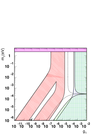
Figure 5: Bounds on Majoron models in the $g_{1}-m_{1}$ plane for the case of the LOW solution ($\Delta m^{2}_{\odot}=10^{-7}eV^{2}$ and $\tan^{2}\theta_{\odot}\simeq 0.67$).

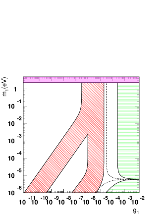
Figure 6: Bounds on Majoron models in the $g_{1}-m_{1}$ plane for the vacuum solution of the solar neutrino problem ($\Delta m^{2}_{\odot}=10^{-10}$ eV² and $\sin^{2}2\theta_{\odot}\simeq 0.9$. The bounds from neutrino spectra don’t apply, since already pure neutrino oscillations implied by the vacuum solution parameters lead to a contradiction with the observed neutrino spectrum of SN1987A.

It is important to notice that the shape of such regions is characterized by the values of the square root of $\Delta m^{2}_{\odot}$ and $\Delta m^{2}_{atm}$. Let us first consider $\tilde{g}_{ij}$ with $i,j\neq 3$. In this case only $\Delta m^{2}_{\odot}$ appears in eq. (17), so that for $m_{1}\gg\Delta m^{2}_{\odot}$ one has $g_{2}\sim g_{1}$ giving rise to a vertical line with no dependence on $m_{1}$, as noted in the figures. In contrast, for $m_{1}\ll\Delta m^{2}_{\odot}$ one has $g_{2}\sim g_{1}\frac{\sqrt{\Delta m^{2}_{\odot}}}{m_{1}}$ with a explicit dependence on $m_{1}$ which strengthens the bound for lower $m_{1}$ values. Let us now consider the limit coming from $g_{3}$. In this case the characteristic mass scale is always given by $\Delta m^{2}_{atm}$, eq. (17), irrespective of the particular solutions to solar neutrino problem that one may wish to consider. As a result, for the LOW and (quasi)–vacuum cases the difference between $\Delta m^{2}_{atm}$ and the solar mass scale $\Delta m^{2}_{\odot}$ is so large that two branches appear. This explains the two branches observed in figures 5 and 6 corresponding to the LOW and (quasi)–vacuum solutions, respectively (section 4).

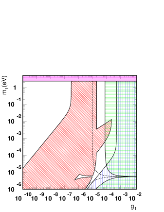
Figure 4: Bounds on Majoron models in the $g_{1}-m_{1}$ plane for the case of the SMA solution ($\Delta m^{2}_{\odot}=10^{-5}$ eV² and $\sin^{2}2\theta_{\odot}\simeq 7\times 10^{-3}$).

Concerning the SMA solution in fig. 4 the main changes arise from the bounds on $|g_{ee}|$ and $|g_{e\mu^{\prime}}|$. In the expression of $g_{ee}$ in eq. (10) the contributions of $g_{1}$ and $g_{2}$ may cancel for a phase $\delta\simeq\pi/2$, see fig. 1, as long as these contributions are of comparable magnitude. To fulfill this requirement, a smaller admixture of $g_{2}$ in $g_{ee}$, as happens for the SMA solution, has to be compensated by a larger ratio of $g_{2}/g_{1}$, corresponding to smaller masses $m_{1}$. This is producing a small hollow in the bound at $m_{1}\sim 5\times 10^{-6}$.

The bound on $|g_{e\mu^{\prime}}|$ is responsible for the sharp peak at the right edge of the excluded region, as can be seen in fig. 2, where all Majoron luminosity bounds are shown explicitly. Here the conservative upper bound on $|g_{e\mu^{\prime}}|$ is obtained, when $\delta=0$, corresponding to cancellation of the $g_{1}$ and $g_{2}$ contributions in the large $m_{1}^{2}$ asymptotics, see eq. (10). Correspondingly the right border of the excluded region is obtained for $\delta=\pi/2$, where $|g_{e\mu^{\prime}}|$ becomes constant for large $m_{1}$. The intersection gives rise to the peak. For smaller values of the mixing, as obtained for the SMA solution, the expression for $|g_{e\mu^{\prime}}|$ in eq. (10) is fulfilled for corresponding larger values of $g_{1}$. This shifts the exclusion region to the right, making it more visible in fig. 4.

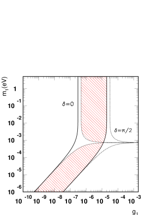
Figure 1: Excluded regions from the Majoron luminosity requirement $3\times 10^{-7}<|g_{ee}|<2\times 10^{-5}$, for two extreme CP cases, $\delta=0$ (solid lines) and $\delta=\pi/2$ (dotted lines), in the $m_{1}-g_{1}$ plane. LMA parameters $\sin^{2}(2\theta)=0.6~{},~{}~{}\Delta m^{2}_{\odot}=1\times 10^{-5}$ eV² are assumed.

Figure 2: Excluded regions independent of CP phase from the Majoron luminosity requirement on $|g_{ee}|$, (solid line), $|g_{e\mu^{\prime}}|$ (dashed line), $|g_{\mu^{\prime}\mu^{\prime}}|$ (dotted lines) and $|g_{\tau^{\prime}\tau^{\prime}}|$ (dash-dotted line), in the $m_{1}-g_{1}$ plane. LMA parameters $\sin^{2}(2\theta)=0.6~{},~{}~{}\Delta m^{2}_{\odot}=1\times 10^{-5}$ eV² are assumed.

Before concluding this section we mention the constraints on Majoron-neutrino coupling parameters which arise from the collapsing phase. The idea behind this bound is that a change in the trapped electron fraction could prevent a successful explosion process. At the end of their life massive stars become unstable and, when the iron core reaches the Chandrasekar limit, they implode. Once the nuclear density is reached, a shock wave forms at the core and propagates outwards, turning the implosion into an explosion. The strength and propagation of this shock is sensitive to the trapped electron fraction $Y_{L_{e}}=Y_{e}+Y_{\nu_{e}}$, which can be erased by neutrino decays $\nu_{e}\to\overline{\nu}_{e}+J$. Requiring $Y_{L}(t_{bounce})>0.375$ leads to a limit of [12]

$$|g_{ee}|<2\times 10^{-6}.$$ (24)

However to the extent that current supernova models do not fully account for the explosion mechanism this limit should be taken only as indicative for the moment.

4 Neutrinoless double beta decay

The only laboratory experiment, which is competitive with the supernova bounds, is neutrinoless double beta decay. This decay corresponds to two single beta decays occuring in one nucleus and converts a nucleus (Z,A) into a nucleus (Z+2,A). Limits on the Majoron emitting mode

$${}^{A}_{Z}X\to^{A}_{Z+2}X+2e^{-}+\phi$$ (25)

are given by two types of experiments. In geochemical experiments the half–life limit is derived from relative abundances of nuclear isotopes found in the earth [22]:

$$|g_{ee}|<3\times 10^{-5}.$$ (26)

However, half–life determinations vary by more than a factor of three.

The best direct laboratory limit (less stringent but more reliable) from the Heidelberg-Moscow experiment [23] is based on a likelyhood fit to the continuous electron spectrum:

$$|g_{ee}|<8\times 10^{-5}.$$ (27)

Future projects such as GENIUS [16] and EXO [24] aim at considerable improvements in the sensitivity. A very rough estimation of the sensitivity of GENIUS 1t is based on the background simulation in [16], where a background improvement in the interesting energy range of a factor $\sim 1000$ has been obtained. Since in the Heidelberg-Moscow experiment the Majoron-neutrino coupling bounds are dominated by the systematical error of the background simulation, a considerable reduction of the background by a factor of $B$ will reduce the limit on the Majoron-emitting double beta decay half life by $\sim\sqrt{B}$ and the coupling constant limit accordingly by $\sim^{4}\sqrt{B}$. This implies a reach of sensitivity down to $|g_{ee}|\sim 10^{-5}$, which could bridge most of the gap existing between the more reliable limits derived from supernovae.

5 Discussion and conclusions

In figures 3 to 6 we present the limits on Majoron-neutrino couplings in terms of $m_{1}-g_{1}$ corresponding to the various solutions of the solar neutrino problem. In Fig. 7 we display the results for the LMA solution also in terms of the equivalent $m_{2}-g_{2}$ variables. This representation has been selected for convenience and generality. By further specifying the underlying model for lepton number violation one can re-express our results in terms of the lepton number breaking VEV, which will provide also useful information for model-builders.

Regions which are excluded by supernova arguments are denoted by the rhombical pattern (obtained from Majoron luminosity) and by the vertical lines (obtained from the neutrino spectra). Also shown are the regions excluded from neutrinoless double beta decay (horizontal lines). The excluded region from Majoron luminosity is a superposition of the bounds on $\tilde{g}_{11}$, $\tilde{g}_{12}$, $\tilde{g}_{22}$, and $\tilde{g}_{33}$, where always the most conservative limits for various CP Majorana phases have been used. Due to the expressions for the helicity-flipping neutrino decays the bound obtained from the neutrino spectra turns out to be independent of the CP phase. For neutrinoless double beta decay one can have a cancellation of the coupling constants $g_{1}$ and $g_{2}$. The expected sensitivity of the GENIUS experiment is shown as a dashed line. It is easy to see that GENIUS could be able to bridge almost the whole gap between the different supernova constraints. Also an upper bound $m_{1}<2.3$ eV from tritium beta decay is displayed.

The limits obtained in this paper apply to the simplest class of models where neutrino masses arise from the spontaneous violation of lepton number. Such Majoron models which cover a wide and attractive class including both models where the smallness of neutrino masses follow from a seesaw scheme, as well as those where it arises from the radiative corrections.

Both neutrinoless double beta decay as well as supernova physics arguments provide stringent limits on Majoron-neutrino interactions. In the present work we have discussed these limits and their translation into the mass basis. Generalizing previous papers [12] we have now taken into account the effect of CP violating phases, which play a crucial role in the neutrinoless double beta decay limits. Depending on the solution of the solar neutrino problem and the absolute mass scale in the neutrino sector the constraint from the supernova energy release (Majoron luminosity argument) exludes Majoron-neutrino couplings in the wide range of $10^{-7}-10^{-5}$. Upper bounds have been obtained from neutrinoless double beta decay and the SN87A neutrino spectra. An estimate of the potential of the future double beta projects such as GENIUS suggests the possibility to bridge almost the whole gap separating the excluded areas and either to establish Majorons with couplings around a few $10^{-5}$ or to restrict neutrino-Majoron couplings down to $10^{-7}$.

Last, but not least, let us mention that the propagation of neutrinos produced in the solar interior follows essentially the MSW picture, while any possible effect of decays would happen in vacuo through a non-diagonal neutrino-majoron coupling which is absent in the simplest models considered here [4]. Even in more complex models [9, 10] where such non-diagonal neutrino-majoron couplings exist in vacuo, one can see that for such small values of the neutrino-majoron coupling strengths indicated by supernova and neutrinoless double beta decay, it is rather unlikely that they can play any role whatsoever in the solar neutrino problem [25].

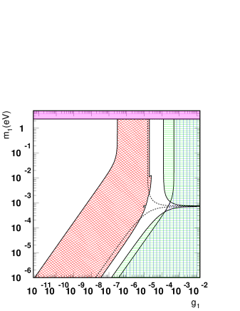
Figure 3: Bounds on Majoron models in the $g_{1}-m_{1}$ plane for the case of the LMA solution ($\Delta m^{2}_{\odot}=10^{-5}$ eV² and $\sin^{2}2\theta_{\odot}\simeq 0.6$).

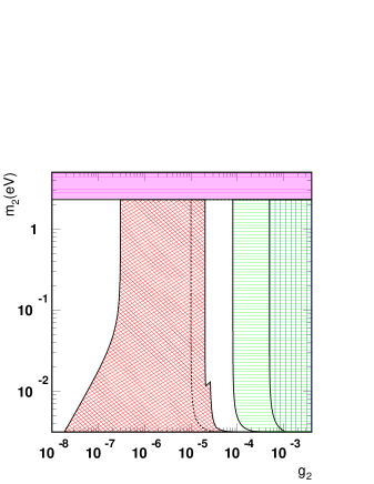
Figure 7: Bounds on Majoron models expressed in terms ofthe $g_{2}-m_{2}$ for the case for the LMA solution of the solar neutrino problem.

References

- [1] H. Sobel, http://nu2000.sno.laurentian.ca; T. Toshito, http://www.ichep2000.rl.ac.uk. Y. Fukuda et al. [SuperKamiokande Collaboration], Phys. Rev. Lett. 81 (1998) 1562; Phys. Rev. Lett. 82 (1999) 2644 [hep-ex/9812014]. Y. Fukuda et al., Phys. Lett. B433, 9 (1998); Phys. Lett. B436, 33 (1998); For a recent analysis see: N. Fornengo, M.C. Gonzalez-Garcia, J. W. F. Valle, Nucl. Phys. B580 (2000) 58-82 [hep-ph/0002147]
- [2] Y. Suzuki, talk at XIX International Conference on Neutrino Physics and Astrophysics, Sudbury, Canada, http://nu2000.sno.laurentian.ca; T. Takeuchi, talk at the XXXth International Conference on High Energy Physics, ICHEP 2000 http://www.ichep2000.rl.ac.uk. Homestake Collaboration, B.T. Cleveland et al., Astrophys. J. 496, 505 (1998); R. Davis, Prog. Part. Nucl. Phys. 32, 13 (1994); K. Lande, http://nu2000.sno.laurentian.ca; SAGE Collaboration, J.N. Abdurashitov et al., Phys. Rev. C60, 055801 (1999); V. Gavrin, http://nu2000.sno.laurentian.ca. GALLEX Collaboration, W. Hampel et al., Phys. Lett. B447, 127 (1999). E. Belloti, http://nu2000.sno.laurentian.ca. For a recent analysis see: M. C. Gonzalez-Garcia, P. C. de Holanda, C. Pena-Garay and J. W. F. Valle, Nucl. Phys. B573 (2000) 3 [hep-ph/9906469]
- [3] M. C. Gonzalez-Garcia, M. Maltoni, C. Pena-Garay and J. W. F. Valle, Phys. Rev. D 63 (2001) 033005 [hep-ph/0009350].
- [4] Y. Chikashige, R.N. Mohapatra and R.D. Peccei, Phys. Lett. B 98 (1981) 26
- [5] Two basic types of radiative neutrino mass models were considered in A. Zee, Phys. Lett. B 93, 3890 (1980) and K. S. Babu, Phys. Lett. B 203, 132 (1988). For Majoron embeddings of these models see, for example, A. S. Joshipura and J. W. F. Valle, Nucl. Phys. B 397, 105 (1993).
- [6] A. Masiero and J. W. F. Valle, Phys. Lett. B251 (1990) 273
- [7] J.W.F. Valle, Gauge Theories and the Physics of Neutrino Mass, Progr. Part. Nucl. Phys. 26 (1991) 91-171
- [8] J. Schechter and J. W. F. Valle, Phys. Rev. D 25 (1982) 774.
- [9] M. C. Gonzalez-Garcia and J. W. F. Valle, Phys. Lett. B 216 (1989) 360.
- [10] G. B. Gelmini and J. W. F. Valle, Phys. Lett. B 142 (1984) 181.
- [11] M. Hirsch, H.V. Klapdor–Kleingrothaus, S.G. Kovalenko, H. Päs, Phys. Lett. B 372 (1996) 8; M. Hirsch. H. V. Klapdor–Kleingrothaus, B. Maier, H. Päs, in Proc. Int. Workshop on Double Beta Decay and Related Topics, Trento, 24.4.–5.5.95, World Scientific Singapore, Ed.: H.V. Klapdor–Kleingrothaus and S. Stoica
- [12] M. Kachelriess, R. Tomàs, J.W.F. Valle, Phys. Rev. D 62 (2000) 023004 [hep-ph 0001039]
- [13] C. Giunti, C.W. Kim, U.W. Lee, W.P. Lam, Phys. Rev. D 45 (1992) 1557
- [14] J. Schechter and J.W.F. Valle, Phys. Rev. D22 (1980) 2227.
- [15] J. Schechter and J. W. F. Valle, Phys. Rev. D 23 (1981) 1666.
- [16] H.V. Klapdor–Kleingrothaus, Proc. Beyond the Desert ’97; J. Hellmig, H.V. Klapdor–Kleingrothaus, Z. Phys. A 359 (1997) 351; H.V. Klapdor–Kleingrothaus, M. Hirsch, Z. Phys. A 359 (1997) 361; H.V. Klapdor–Kleingrothaus, J. Hellmig, M. Hirsch, J. Phys. G 24 (1998) 483; H.V. Klapdor–Kleingrothaus, L. Baudis, G. Heusser, B. Majorovits, H. Päs, hep-ph/9910205
- [17] P.D. Mannheim, Phys. Rev. D37, 1935 (1988).
- [18] M. Apollonio et al., Phys.Lett. B466 (1999) 415, hep-ex/9907037; F. Boehm et al., hep-ex/9912050
- [19] This simplified form of the lepton mixing matrix was first given in J. Schechter and J.W.F. Valle, Phys. Rev. D21, 309 (1980).
- [20] A.Yu. Smirnov, D.N. Spergel and J.N. Bahcall, Phys. Rev. D49 (1994) 1389.
- [21] B. Jegerlehner, F: Neubig and G. Raffelt, Phys. Rev. D54 (1996) 1194.
- [22] T. Bernatowicz et al., Phys. Rev. Lett. 69 (1992) 2341
- [23] H.V. Klapdor–Kleingrothaus et al. (Heidelberg–Moscow Collab) hep-ph/0103062; L. Baudis, priv. comm.
- [24] M. Danilov et al., Phys.Lett. B480 (2000) 12-18
- [25] J. N. Bahcall, S. T. Petcov, S. Toshev and J. W. Valle, Phys. Lett. B 181 (1986) 369. For a recent paper see, e. g. A. Bandyopadhyay, S. Choubey and S. Goswami, Phys. Rev. D 63 (2001) 113019