Radiative decays of mesons in the NJL model

Abstract

We revisit the theoretical predictions for anomalous radiative decays of pseudoscalar and vector mesons. Our analysis is performed in the framework of the Nambu–Jona-Lasinio model, introducing adequate parameters to account for the breakdown of chiral symmetry. The results are comparable with those obtained in previous approaches.

I Introduction

The analysis of vector and axial-vector meson physics represents a nontrivial task from the theoretical point of view. This is basically due to the characteristic energy scales at which these particles manifest, namely an intermediate range between low energy hadron physics and the high energy region where QCD can be treated perturvatively. In order to deal with the subject, one possible approach is to start from an effective meson Lagrangian; another possible way is to derive the corresponding effective interactions from QCD-inspired fermionic schemes.

In the last two decades, the development of chiral effective models [1] has provided a profitable framework to analyze various phenomena related to the physics of vector and axial-vector mesons [2, 3, 4]. These models have been built taking into account the symmetries of QCD, together with the so–called axial anomaly introduced through the Wess-Zumino-Witten (WZW) [5] effective action. As an alternative approach, the analysis of spin one meson physics can be performed by starting with the Lagrangian proposed by Nambu and Jona–Lasinio (NJL) [6]. This Lagrangian is based in 4-fermion interactions, showing the chiral symmetry of QCD, and leads to an effective theory for scalar, pseudoscalar, vector and axial–vector mesons after proper bosonization. The effective meson Lagrangian can be obtained by constructing a generating functional, and evaluating the real and imaginary parts of the fermion determinant [7].

In this work we follow this second approach, studying the phenomenology of spin 1 mesons in the framework of the NJL model. We propose a fermionic Lagrangian that shows an approximate $U(3)_{L}\otimes U(3)_{R}$ chiral symmetry, explicitly violated by current quark masses, as is the case of QCD in the limit of large number of colours $N_{C}$. In particular, we revisit the predictions given by this model for anomalous radiative decays of vector mesons, taking into account the explicit breakdown of the $SU(3)$ flavour symmetry to $SU(2)$ isospin symmetry with the assumption $m_{u}=m_{d}\neq m_{s}$. We perform the bosonization of the NJL theory by carrying out an expansion of the fermion determinant in terms of the meson fields. This gives rise to a set of one–loop Feynman diagrams [8, 9, 10, 11, 12] from which one can derive the relevant effective meson interactions. Taking into account present experimental data, we analyze possible input parameters for the model, in order to obtain an acceptable phenomenological pattern for the observed anomalous decays of pseudoscalar and vector mesons.

The paper is organized as follows: In Sect. II we introduce the NJL Lagrangian and the bosonization technique. In Sect. III we derive the effective Lagrangian to account for vector and axial-vector meson interactions, considering the explicit breakdown of flavour $SU(3)$ symmetry. This leads to some relations between vector meson masses and decay constants that can be written in terms of symmetry breaking parameters. Then, in Sect. IV, we concentrate on the anomalous radiative decays of pseudoscalar and vector mesons, which proceed through the $U(1)$ axial anomaly. In Sect. V we discuss the numerical results for the corresponding branching ratios, in comparison with the present experimental information. Finally in Sect. VI we present our conclusions. The Appendix includes a brief description of the regularization scheme used throughout our analysis.

II Nambu–Jona–Lasinio Lagrangian and bosonization

Chiral effective models have proved to reproduce the low energy hadron phenomena with significant success. For that reason, a significant effort has been done in order to derive these effective schemes from a microscopic theory as QCD. The effective four fermion Lagrangian proposed by Nambu and Jona–Lasinio [6], which shows the chiral symmetry of QCD, represents one of the most popular ways to achieve this goal. The NJL model provides, after proper bosonization, not only the expected effective couplings for scalar, pseudoscalar, vector and axial–vector mesons but also the Wess–Zumino–Witten sector [5] which accounts for the anomalous meson decays. The explicit form of the NJL Lagrangian reads

$${\cal L} = \bar{q}(i\not\!\partial-\hat{m}_{0})q+2G_{1}\left[(\bar{q}\frac{1}{2}\lambda^{a}q)^{2}+(\bar{q}i\gamma_{5}\frac{1}{2}\lambda^{a}q)^{2}\right]$$ (2)

$$-2G_{2}\left[(\bar{q}\gamma^{\mu}\frac{1}{2}\lambda^{a}q)^{2}+(\bar{q}\gamma^{\mu}\gamma_{5}\frac{1}{2}\lambda^{a}q)^{2}\right],$$

where $q$ denotes the $N$-flavour quark spinor, $\lambda^{a}$, $a=0,\dots,N^{2}-1$ are the generators of the $U(N)$ flavour group (we normalize $\lambda^{0}=\sqrt{2/N}\,\openone$) and $\hat{m}_{0}$ stands for the current quark mass matrix, which explicitly breaks the chiral symmetry. The coupling constants $G_{1}$ and $G_{2}$, as well as the quark masses, are introduced as free parameters of the model. In the absence of the mass term, the NJL Lagrangian shows at the quantum level the $SU(N)_{A}\otimes SU(N)_{V}\otimes U(1)_{V}$ symmetry characteristic of massless QCD.

It is possible to reduce the fermionic degrees of freedom to bosonic ones by standard bosonization techniques. With the introduction of colorless boson fields and an appropriate use of the Stratonovich identity, one obtains an effective action where the fermions couple to the bosons in a bilinear form. The couplings driven by $G_{1}$ in (2) lead to the introduction of scalar and pseudoscalar boson fields, whereas those carrying $G_{2}$ lead to the inclusion of vector and axial–vector mesons.

To be definite, let us consider the vector meson sector with $N=3$ flavours, $u$, $d$ and $s$. By means of the Stratonovich identity, the vector–vector coupling in (2) can be transformed as

$$-2G_{2}(\bar{q}\gamma^{\mu}\frac{1}{2}\lambda^{a}q)^{2}\rightarrow-\frac{1}{4G_{2}}\mbox{Tr}\,V_{\mu}^{2}+i\bar{q}\gamma^{\mu}V_{\mu}q,$$ (3)

where $V_{\mu}\equiv-i\displaystyle\sum_{a=0}^{8}V_{\mu}^{a}\;\lambda^{a}/2$. The spin 1 fields $V_{\mu}^{a}$ can be identified with the usual nonet of vector mesons,

$$V=\frac{(-i)}{\sqrt{2}}\left(\begin{array}[]{ccc}\displaystyle\frac{\rho^{0}}{\sqrt{2}}+\frac{\omega_{8}}{\sqrt{6}}+\frac{\omega_{1}}{\sqrt{3}}&\rho^{+}&K^{*+}\\ \rho^{-}&\displaystyle-\frac{\rho^{0}}{\sqrt{2}}+\frac{\omega_{8}}{\sqrt{6}}+\frac{\omega_{1}}{\sqrt{3}}&K^{*0}\\ K^{*-}&{\bar{K}}^{*0}&\displaystyle-\frac{2\,\omega_{8}}{\sqrt{6}}+\frac{\omega_{1}}{\sqrt{3}}\end{array}\right)\,$$ (4)

which transform in such a way to preserve the chiral symmetry of the original NJL Lagrangian (and therefore that of QCD). Notice that the first term in the right hand side of Eq. (3) is nothing but a mass term for the vector fields $V_{\mu}^{a}$, thus the vector–meson masses are governed by the coupling $G_{2}$ in the NJL Lagrangian. It can be seen that these masses are degenerate in the limit where the quark masses are degenerate.

Now, the quark fields can be integrated out, leading to an effective Lagrangian which only contains bosonic degrees of freedom. This procedure can be carried out by taking into account the generating functional

$${\cal Z}={\cal N}\int{\cal D}V{\cal D}q{\cal D}{\bar{q}}\;\exp\left\{i\int dx^{4}\left[-\frac{1}{4G_{2}}\mbox{Tr}\,V_{\mu}^{2}+{\bar{q}}(i\not\!\partial-{\hat{m}_{0}}+i\not\!V)q\right]\right\}$$ (5)

and performing the calculation of the fermion determinant (a detailed analysis can be found in [7]). A similar procedure can be followed for the full NJL Lagrangian (2), leading to the interactions involving scalar, pseudoscalar and axial–vector bosons. In this way, the final effective Lagrangian is written only in terms of spin 0 and spin 1 colorless hadron fields.

Here we have performed the bosonization by carrying out an expansion of the fermion determinant, which gives rise to a set of one–loop Feynman diagrams [8]. In order to build up the final effective meson Lagrangian, we have obtained the local part of the relevant interactions by taking the leading order of a gradient expansion in powers of the external momenta, and considering the dominant contributions in $1/N_{C}$. The divergent integrals have been treated using a proper–time regularization scheme with a momentum cut–off, keeping the leading contributions. The procedure is developed in detail in the next section.

III Effective meson couplings and symmetry-breaking parameters

In this section we describe the effective meson interactions derived from the NJL Lagrangian. We begin by calculating the relevant one–loop self–energy diagrams contributing to the meson kinetic and mass terms, and those leading to the effective weak and strong meson decay couplings. Notice that the meson fields introduced through the bosonization technique acquire their dynamics via the self–energy one–loop diagrams.

In our framework, the poles of the quark propagators occur at the so–called constituent masses, i.e. dynamically generated masses which arise as a consequence of the spontaneous breakdown of the chiral symmetry. The constituent masses appear as solutions of Schwinger-Dyson self-consistency equations (gap equations), which are governed by the scalar coupling $G_{1}$ in the NJL Lagrangian (2). Here we will not concentrate in the scalar sector of the model, thus the constituent quark masses, as well as the pseudoscalar boson masses, will be considered as free parameters.

Our main interest is focused in the anomalous radiative decays of vector mesons. Nevertheless, we need to consider also the axial–vector sector of the model, since the axial–vectors mix with the pseudoscalars at the one–loop level ($P-A$ mixing).

A Kinetic terms and masses of the spin-1 mesons

The generating functional (5) gives rise to effective kinetic terms for the spin-1 vector mesons via one–loop diagrams, as shown in Fig. 1(a). The analysis in the case of the axial–vector mesons can be performed in an analogous way, with the additional ingredient of $P-A$ mixing given by Fig. 1(b).

The loop in Fig. 1(a) gives a contribution to the vector meson self-energy given by

$$iN_{C}\int\frac{d^{4}k}{(2\pi)^{4}}\mbox{Tr}\,\frac{\not\!k-\not\!p+m_{1}}{(k-p)^{2}-m_{1}^{2}}\lambda^{a}\gamma_{\mu}\frac{\not\!k+m_{2}}{k^{2}-m_{2}^{2}}\lambda^{b}\gamma_{\nu}\;,$$ (6)

where $m_{1}$ and $m_{2}$ are the constituent masses of the quarks entering the loop, $N_{C}$ is the number of colors, and the trace acts over the flavour and Dirac indices.

As stated above, we will take only the leading order in the external momentum $p$, which means to evaluate the integral at $p=0$ after extracting the relevant kinematical factors. In this case, this is equivalent to consider only the divergent piece of (6):

$$\Pi_{\mu\nu}^{(V)}=I_{2}(m_{1},m_{2})\,\left[\frac{1}{3}\,(p_{\mu}p_{\nu}-p^{2}g_{\mu\nu})+\frac{1}{2}\,(m_{2}-m_{1})^{2}\right]\,,$$ (7)

where

$$I_{2}(m_{i},m_{j})\equiv-i\,\frac{N_{C}}{(2\pi)^{4}}\int d^{4}k\frac{1}{(k^{2}-m_{i}^{2})(k^{2}-m_{j}^{2})}\,.$$ (8)

As it was previously mentioned, in order to regularize the divergence we use the proper–time regularization scheme [13] with a cut–off $\Lambda$, which will be treated as a free parameter of the model. Details of the procedure can be found in the Appendix. We obtain

$$I_{2}(m_{i},m_{j})=\frac{N_{C}}{16\pi^{2}}\int_{0}^{1}dx\;\Gamma\left(0,\frac{(m_{i}^{2}-m_{j}^{2})x+m_{j}^{2}}{\Lambda^{2}}\right)\,.$$ (9)

From (7), the kinetic terms for the vector mesons in the effective Lagrangian are given by

$${\cal L}_{kin}^{(V)} = -\frac{1}{4}\,\frac{2}{3}\,I_{2}(m_{u},m_{u})\left[\rho_{\mu\nu}\rho^{\mu\nu}+2\rho^{+}_{\mu\nu}{\rho^{-}}^{\mu\nu}+\omega_{\mu\nu}\omega^{\mu\nu}+\alpha\,\phi_{\mu\nu}\phi^{\mu\nu}\right.$$ (11)

$$\left.+2\beta\left({K^{\ast}}^{+}_{\mu\nu}{K^{\ast}}^{-\mu\nu}+{K^{\ast}}^{0}_{\mu\nu}\bar{K}^{\ast 0\mu\nu}\right)\right]\,,$$

where $V^{\mu\nu}\equiv\partial^{\mu}V^{\nu}-\partial^{\nu}V^{\mu}$, and

$$\alpha=\frac{I_{2}(m_{s},m_{s})}{I_{2}(m_{u},m_{u})}\;,\qquad\qquad\beta=\frac{I_{2}(m_{u},m_{s})}{I_{2}(m_{u},m_{u})}$$ (12)

parameterize the magnitude of the $SU(3)$ flavour symmetry breaking.

The kinetic Lagrangian in (11) has been expressed in terms of the vector fields in (4), with the additional rotation

$$\omega_{8} = \phi\cos\theta_{0}+\omega\sin\theta_{0}$$ (13)

$$\omega_{1} = -\phi\sin\theta_{0}+\omega\cos\theta_{0}\;\;,$$ (14)

which diagonalizes the neutral sector. It is easy to see that here the rotation is “ideal”, i.e., the spin 1 mass eigenstates $\rho$ and $\omega$ are composed by pure light $u$ and $d$ quarks, while the $\phi$ meson is a bound state $\bar{s}s$. The $\omega-\phi$ rotation angle is given by $\sin\theta_{0}=1/\sqrt{3}$. Slight deviations from the ideal mixing condition will be considered below to allow for the decay $\phi\to\pi^{0}\gamma$ observed recently.

The mass terms for the vector mesons are given by the $(V_{\mu})^{2}$ term in (3), plus a divergent one–loop contribution given by the second term in the square brackets in (7), which vanishes in the $SU(3)$ flavour limit. This leads to

$${\cal L}_{mass}^{(V)} = \frac{1}{8G_{2}}\left[\rho_{\mu}\rho^{\mu}+2\rho^{+}_{\mu}{\rho^{-}}^{\mu}+\omega_{\mu}\omega^{\mu}+\phi_{\mu}\phi^{\mu}+2{K^{\ast}}^{+}_{\mu}{K^{\ast}}^{-\mu}+2{K^{\ast}}^{0}_{\mu}\bar{K}^{\ast 0\mu}\right]$$ (16)

$$+(m_{s}-m_{u})^{2}\beta\,I_{2}(m_{u},m_{u})({K^{\ast}}^{+}_{\mu}{K^{\ast}}^{-\mu}+{K^{\ast}}^{0}_{\mu}\bar{K}^{\ast 0\mu})\;.$$

Notice that (as expected) the mass terms turn out to be diagonal in the ($\omega,\phi$) basis.

We proceed now to the wave function renormalization required by the kinetic terms in (11). The vector meson fields can be properly redefined by $V_{\mu}\to Z^{1/2}_{V}\,V_{\mu}$, with

$$Z_{\rho}^{-1} = Z_{\omega}^{-1}=\frac{2}{3}\,I_{2}(m_{u},m_{u})$$ (18)

$$Z_{K^{\ast}}^{-1} = \frac{2}{3}\,\beta\,I_{2}(m_{u},m_{u})=\beta\,Z_{\rho}^{-1}$$ (19)

$$Z_{\phi}^{-1} = \frac{2}{3}\,\alpha\,I_{2}(m_{u},m_{u})=\alpha\,Z_{\rho}^{-1}\;.$$ (20)

Then from (16) one obtains

$$m_{\rho}^{2}=m_{\omega}^{2}=\frac{Z_{\rho}}{4G_{2}}\;,\qquad m_{K^{*}}^{2}=\frac{m_{\rho}^{2}}{\beta}+\frac{3}{2}(m_{s}-m_{u})^{2}\;,\qquad m_{\phi}^{2}=\frac{m_{\rho}^{2}}{\alpha}\;,$$ (21)

thus the $\phi$ meson mass can be written in terms of the $\rho$ mass and the flavour symmetry breaking parameter $\alpha$. In the case of the $K^{\ast}$, the corresponding mass relation includes both the parameter $\beta$ and a quark–mass dependent contribution that arises from the loop in Fig. 1 (a).

A similar analysis can be performed for the axial–vector meson sector. By replacing $\gamma_{\alpha}\to\gamma_{\alpha}\gamma_{5}$ in the quark–meson vertices in Fig. 1 (a), one finds

$$\Pi_{\mu\nu}^{(A)}=\frac{2}{3}\,I_{2}(m_{1},m_{2})\,\left[(p_{\mu}p_{\nu}-p^{2}g_{\mu\nu})-\frac{3}{2}\,\frac{(m_{2}+m_{1})^{2}}{2}\right]\,,$$ (22)

leading to the kinetic Lagrangian

$${\cal L}_{kin}^{(A)} = -\frac{1}{4}\,\frac{2}{3}I_{2}(m_{u},m_{u})\left[{a_{1}}_{\mu\nu}a_{1}^{\mu\nu}+2{a_{1}}_{\mu\nu}^{+}a_{1}^{-\mu\nu}+f_{1\mu\nu}f_{1}^{\mu\nu}\right.$$ (24)

$$\left.+2\beta{K^{+}_{1}}_{\mu\nu}K_{1}^{-\mu\nu}+2\beta K^{0}_{1\mu\nu}{\bar{K}}_{1}^{0\mu\nu}+\alpha f^{\prime}_{1\mu\nu}{f^{\prime}}_{1}^{\mu\nu}\right]$$

and the mass terms

$${\cal L}_{mass}^{(A)} = \frac{1}{8G_{2}}\left[{a_{1}}_{\mu}a_{1}^{\mu}+2{a_{1}^{+}}_{\mu}a_{1}^{-\mu}+f_{1\mu}f_{1}^{\mu}+f^{\prime}_{1\mu}{f^{\prime}}_{1}^{\mu}+2{K^{+}_{1}}_{\mu}K_{1}^{-\mu}+2K^{0}_{1\mu}{\bar{K}}_{1}^{0\mu}\right]$$ (27)

$$+I_{2}(m_{u},m_{u})\left[2m_{u}^{2}({a_{1}}_{\mu}a_{1}^{\mu}+2{a_{1}^{+}}_{\mu}a_{1}^{-\mu}+f_{1\mu}f_{1}^{\mu})\right.$$

$$\left.+(m_{u}+m_{s})^{2}\beta({K_{1}}_{\mu}^{+}K_{1}^{-\mu}+{K_{1}}_{\mu}^{0}\bar{K}_{1}^{0\mu})+2m_{s}^{2}\alpha f^{\prime}_{1\mu}{f^{\prime}}_{1}^{\mu}\right]\,.$$

As in the vector meson case, the Lagrangian is diagonal in the chosen basis, where $f_{1}$ and ${f^{\prime}}_{1}$ are obtained from the $U(3)$ states $A_{8}$ and $A_{1}$ through an ideal rotation. Notice that both neutral and charged axial–vector boson masses receive a contribution proportional to $G_{2}^{-1}$, which arises from field transformations as in Eq. (3), plus additional (positive) contributions proportional to the quark masses. In this way, the axial–vector mesons are in general expected to be heavier than their vector meson counterparts.

Finally, we have to take into account the mixing between the axial–vector mesons and the pseudoscalars. This requires the analysis of the pseudoscalar–axial vector couplings and the pseudoscalar kinetic terms, given by the one–loop diagrams in Fig. 1 (b) and (c) respectively. The effective couplings read

$${\cal L}_{mix} = -iI_{2}(m_{u},m_{u})\left[2m_{u}(\partial_{\mu}\pi^{0}a_{1}^{\mu}+\partial_{\mu}\pi^{+}a_{1}^{-\mu}+\partial_{\mu}\pi^{-}a_{1}^{+\mu}+\partial_{\mu}\eta_{u}f^{\mu})\right.$$ (30)

$$+\left.\beta(m_{u}+m_{s})(\partial_{\mu}K^{+}K_{1}^{\mu-}+\partial_{\mu}K^{-}K_{1}^{\mu+}+\partial_{\mu}K^{0}\bar{K}_{1}^{0\mu}+\partial_{\mu}\bar{K}^{0}K_{1}^{0\mu})\right.$$

$$+\left.2\alpha m_{s}\partial_{\mu}\eta_{s}f^{\prime\mu}\right]\,,$$

while the pseudoscalar kinetic Lagrangian is given by

$${\cal L}_{kin}^{(P)} = -\frac{1}{2}I_{2}(m_{u},m_{u})\left[\partial_{\mu}\pi^{0}\partial^{\mu}\pi^{0}+2\partial_{\mu}\pi^{+}\partial^{\mu}\pi^{-}+\partial_{\mu}\eta_{u}\partial^{\mu}\eta_{u}+\alpha\,\partial_{\mu}\eta_{s}\partial^{\mu}\eta_{s}\right.$$ (32)

$$+\left.2\beta\,\partial_{\mu}K^{+}\partial^{\mu}K^{-}+2\beta\,\partial_{\mu}K^{0}\partial^{\mu}\bar{K}^{0}\right]\,.$$

Once again, we have chosen a basis for the neutral fields in which the states $\eta_{u}$, $\eta_{s}$ are obtained from the $U(3)$ states $\eta_{8}$, $\eta_{1}$ through an ideal rotation. However, these states cannot be treated as approximate mass eigenstates due to the presence of the $U(1)_{A}$ anomaly, which breaks the $U(3)$ symmetry down to $SU(3)$. Although formally of order $1/N_{C}$, this anomaly leads to a relatively large mass splitting between the observed $\eta$ and $\eta^{\prime}$ physical states. Still, large $N_{C}$ considerations are shown to be powerful enough to deal with the interactions of the $\eta_{1}$ and $\eta_{8}$ fields as members of an $U(3)$ nonet. As stated, we will not concentrate here in the pseudoscalar mass sector, and consequently, in the $U(1)_{A}$ symmetry breaking mechanism responsible for the $\eta^{\prime}$ mass. In the NJL framework, one way to proceed is to include the so-called ’t Hooft interaction [14, 15], which emulates the effect of the anomaly. Instead of following this way (which means to include six-fermion interaction vertices) we will introduce the $\eta-\eta^{\prime}$ mixing angle as a parameter of the model. Thus we write $\eta_{u}$ and $\eta_{s}$ in terms of the physical states as

$$\eta_{u} = \cos\varphi_{P}\;\eta+\sin\varphi_{P}\;\eta^{\prime}$$ (33)

$$\eta_{s} = -\sin\varphi_{P}\;\eta+\cos\varphi_{P}\;\eta^{\prime}\;.$$ (34)

In order to write the effective Lagrangian in terms of the physical fields, one needs not only the relevant wave function renormalizations but also the diagonalization of the $P-A$ couplings. This can be achieved by means of the transformations

$$P\to Z^{1/2}_{P}P\;,\qquad\qquad A_{\mu}\to Z^{1/2}_{A}\,A_{\mu}+C_{P}Z_{P}^{1/2}\,\partial_{\mu}P\;,$$ (35)

where $P=\pi$, $K$, $\eta_{u}$, $\eta_{s}$, and

$$C_{\pi} = i\,2\,I_{2}(m_{u},m_{u})Z_{\rho}\frac{m_{u}}{m_{a_{1}}^{2}}\;=\;C_{\eta_{u}}$$ (36)

$$C_{K} = i\,2\,I_{2}(m_{u},m_{u})Z_{\rho}\frac{(m_{u}+m_{s})}{2\,m_{K_{1}}^{2}}$$ (37)

$$C_{\eta_{s}} = i\,2\,I_{2}(m_{u},m_{u})Z_{\rho}\frac{m_{s}}{m_{f^{\prime}}^{2}}\;.$$ (38)

The wave function renormalization for the pseudoscalar sector yields

$$Z_{\pi}^{-1} = Z_{\eta_{u}}^{-1}=I_{2}(m_{u},m_{u})\left(1-\frac{6m_{u}^{2}}{m^{2}_{a_{1}}}\right)$$ (39)

$$Z_{K}^{-1} = \beta I_{2}(m_{u},m_{u})\left[1-\frac{3}{2}\frac{(m_{u}+m_{s})^{2}}{m^{2}_{K_{1}}}\right]$$ (40)

$$Z_{\eta_{s}}^{-1} = \alpha I_{2}(m_{u},m_{u})\left(1-\frac{6m_{s}^{2}}{m^{2}_{f^{\prime}}}\right),$$ (41)

where the axial–vector meson masses can be read from (27). As can be immediately seen from (24), the wave function renormalization for the axial–vector mesons is equivalent to that performed in the vector meson sector, c.f. Eq. (III A). Using these relations and those in (21), the axial–vector meson masses turn out to be constrained by

$$m_{a_{1}}^{2} = m_{\rho}^{2}+6m_{u}^{2}$$ (42)

$$m_{K_{1}}^{2} = m_{K^{*}}^{2}+6m_{u}m_{s}$$ (43)

$$m_{f^{\prime}}^{2} = m_{\phi}^{2}+6m_{s}^{2}\;.$$ (44)

B Weak and strong decay constants

We want to analyze the ability of the effective model under consideration to describe the low energy behaviour of pseudoscalar and vector mesons. Let us begin by studying some fundamental decay processes, in order to evaluate the relevant decay constants in terms of the model parameters.

The pseudoscalar weak decay constants $F_{\pi}$ and $F_{K}$ can be obtained from the one–loop transitions represented in Fig. 2, where $P=\pi$, $K$. As in the self–energy case, these diagrams are found to be logarithmically divergent and can be regularized using the proper–time scheme. We will keep as before only the leading contributions in the limit of vanishing external momenta, which amounts to take only the divergent piece of the loop integrals.

The decay constants $F_{P}$ are defined as usual by

$$\langle 0|J_{\mu 5}(0)|P(q)\rangle=i\,\sqrt{2}\,F_{P}\,q_{\mu}\;.$$ (45)

It is easy to see that the contributions from Fig. 2 (a) and (b) lead to

$$F_{\pi} = 2\,I_{2}(m_{u},m_{u})m_{u}Z_{\pi}^{1/2}\left(1+i\,2\,m_{u}C_{\pi}\right)$$ (46)

$$= 2\,I_{2}(m_{u},m_{u})m_{u}Z_{\pi}^{1/2}\left(1-6\frac{m_{u}^{2}}{m^{2}_{a_{1}}}\right)$$ (47)

$$F_{K} = \rule{0.0pt}{14.22636pt}I_{2}(m_{u},m_{u})\,\beta\,(m_{u}+m_{s})\,Z_{K}^{1/2}\left[1+i\,(m_{u}+m_{s})C_{K}\right]$$ (48)

$$= \rule{0.0pt}{22.76228pt}I_{2}(m_{u},m_{u})\beta\,(m_{u}+m_{s})Z_{K}^{1/2}\left[1-\frac{3}{2}\frac{(m_{u}+m_{s})^{2}}{m^{2}_{K_{1}}}\right]\;,$$ (49)

where have made use of Eqs. (38). In these equations, the first terms arise from the graph in Fig. 2 (a), whereas the contributions proportional to $C_{\pi,K}$ are due to the $P-A$ mixing diagrams. Using now Eqs. (41), we end up with the simple relations

$$F_{\pi}=\frac{2\,m_{u}}{Z_{\pi}^{1/2}}\;,\qquad\qquad F_{K}=\frac{(m_{u}+m_{s})}{Z_{K}^{1/2}}\;.$$ (50)

Next, let us study the basic decay constants $g_{\rho}$, $g_{K^{\ast}}$ and $g_{\phi}$, which account for the strong decays of the vector mesons into two pseudoscalars. The decay constants can be defined from the total decay rates according to

$$\Gamma(\rho\to\pi\pi) = \frac{g_{\rho}^{2}}{4\pi}\,\frac{m_{\rho}}{12}\left(1-\frac{4m_{\pi}^{2}}{m_{\rho}^{2}}\right)^{3/2}$$ (51)

$$\Gamma(K^{\ast}\to K\pi) = \rule{0.0pt}{22.76228pt}\frac{g_{K^{\ast}}^{2}}{4\pi}\,\frac{m_{K^{\ast}}}{16}\left\{\left[1-\frac{(m_{K}+m_{\pi})^{2}}{m_{K^{\ast}}^{2}}\right]\left[1-\frac{(m_{K}-m_{\pi})^{2}}{m_{K^{\ast}}^{2}}\right]\right\}^{3/2}$$ (52)

$$\Gamma(\phi\to KK) = \rule{0.0pt}{14.22636pt}\Gamma(\phi\to K^{+}K^{-})+\Gamma(\phi\to K^{0}\bar{K}^{0})$$ (53)

$$= \rule{0.0pt}{22.76228pt}\frac{g_{\phi}^{2}}{4\pi}\,\frac{m_{\phi}}{24}\left[\left(1-\frac{4m_{K^{+}}^{2}}{m_{\phi}^{2}}\right)^{3/2}+\left(1-\frac{4m_{K^{0}}^{2}}{m_{\phi}^{2}}\right)^{3/2}\right]\,.$$ (54)

Notice that for the $\phi\to KK$ width we have taken into account the mass difference between the neutral and charged kaons. Though tiny, this mass difference becomes important in view of the very narrow phase space allowed.

Within the effective model analyzed here, the decay rates (54) are dominated by the one–loop graphs shown in Fig. 3. As before, we keep here the dominant, logarithmically divergent contribution, and the leading order in the external momenta (the corresponding diagrams with two axial–vector legs vanish in this limit). From the evaluation of the $\rho\to\pi\pi$ and $\rho\to a_{1}\pi$ diagrams, and using (III A), (38) and (41), we find

$$g_{\rho}=I_{2}(m_{u},m_{u})Z_{\rho}^{1/2}Z_{\pi}\left(1+i\,2\,m_{u}\,C_{\pi}\right)=Z_{\rho}^{1/2}\;.$$ (55)

In the case of $g_{\phi}$ the evaluation of the dominant contribution is more involved, since the loop includes two different quark propagators. The loop integral has the form

$$I_{3}\equiv-i\,\frac{N_{C}}{(2\pi)^{4}}\int d^{4}k\frac{k^{2}}{(k^{2}-m_{u}^{2})(k^{2}-m_{s}^{2})^{2}}\,.$$ (56)

Once again the divergence is logarithmic, thus it is natural to express the integral in terms of $I_{2}(m_{i},m_{j})$. However, owing to the flavour symmetry breakdown, there is an ambiguity at the moment of choosing the infinite part of (56). Here we follow the criterion of respecting the natural hierarchy given by the quark content of the decaying vector meson, that means, we use the $k^{2}$ factor in the integrand to remove the $m_{u}^{2}$ pole. We have then

$$I_{3}\to\alpha\,I_{2}(m_{u},m_{u})\;.$$ (57)

Taking into account the wave function renormalization for the $\phi$ and $K$ mesons, together with the corresponding pseudoscalar–axial vector mixing, we end up with

$$g_{\phi}=\frac{\sqrt{\alpha}}{\beta}\,g_{\rho}\;.$$ (58)

In the same way we proceed for the case of the $K^{\ast}$ to two meson decay. Here, due to the $SU(3)$ symmetry breaking, the analogous of Eq. (55) for $g_{K^{\ast}}$ leads to a relation between $g_{K^{\ast}}$ and $g_{\rho}$ which can be written in terms of $Z_{\pi,K}$ and $C_{\pi,K}$. At first approximation, however, the dependence on these parameters cancels and one can write

$$g_{K^{\ast}}\simeq g_{\rho}\;.$$ (59)

In this way, both $\phi$ and $K^{\ast}$ strong decay constants can be predicted in terms of the measured value of $g_{\rho}$ and the symmetry breaking parameters $\alpha$ and $\beta$. The corresponding numerical evaluation will be done in Sect. V.

IV Anomalous radiative decays of pseudoscalar and vector mesons

Our goal is to test the ability of this relatively simple, NJL–like model to reproduce the observed pattern for the anomalous radiative decays of pseudoscalar and vector mesons once the breakdown of chiral symmetry is taken into account. These decays are mainly originated by the $U(1)_{A}$ anomaly. In the framework of our model, they occur through the well–known triangle graphs shown in Fig. 4, which lead to an anomalous Wess–Zumino–Witten effective Lagrangian. The corresponding diagrams including an axial–vector which mixes with the pseudoscalar meson gives a vanishing contribution [16]. This can be seen e.g. by looking at the effective anomalous Lagrangian obtained by gauging the Wess–Zumino–Witten action, as shown in Ref. [3].

The couplings between the vector mesons and the outgoing (on–shell) photons follow from the assumption of vector meson dominance of the electromagnetic interactions. In our framework, these couplings can be obtained from quark–loop diagrams connecting photons and vector mesons (see Ref. [7, 11] for details). After the proper inclusion of the symmetry breaking parameters $\alpha$ and $\beta$, the $V-\gamma$ couplings read

$$j_{\mu}^{em}=e\,m_{\rho}^{2}\,Z_{\rho}^{-1/2}\left(\rho_{\mu}+\frac{1}{3}\;\omega_{\mu}+\frac{\sqrt{2}}{3}\frac{m_{\phi}^{2}}{m_{\rho}^{2}}\sqrt{\alpha}\;\phi_{\mu}\right)\;.$$ (60)

Let us begin by analyzing the decays of the neutral pseudoscalars $\pi^{0}$, $\eta$ and $\eta^{\prime}$ into two photons. These processes arise at the one–loop level from the triangle diagrams shown in Fig. 4 (a). The diagrams are found to be convergent, and the limit of vanishing external momenta can be taken trivially. For $\pi^{0}\to\gamma\gamma$ we get

$$\Gamma(\pi^{0}\to\gamma\gamma)=\frac{\alpha^{2}m_{\pi}^{3}}{64\pi^{3}}\left(\frac{Z_{\pi}^{1/2}}{2m_{u}}\right)^{2}=\frac{\alpha^{2}m_{\pi}^{3}}{64\pi^{3}F_{\pi}^{2}}\;,$$ (61)

where $\alpha$ is the electromagnetic fine structure constant. This expression coincides with the result obtained in standard Chiral Perturbation Theory [1]. In the case of $\eta$ and $\eta^{\prime}$ decays to two photons, one has the additional problem of $\eta-\eta^{\prime}$ mixing. In our framework, instead of dealing with the $U(3)$ states $\eta_{1}$ and $\eta_{8}$, it is natural to work with the $\eta_{u}$ and $\eta_{s}$ states defined above, which determine the flavour content of the quark propagators in the loop. Taking into account the corresponding pseudoscalar wave–function renormalizations, we find

$$\Gamma(\eta\to\gamma\gamma) = \frac{\alpha^{2}m_{\eta}^{3}}{64\pi^{3}}\left[\frac{5}{3F_{\pi}}\cos\varphi_{P}-\frac{\sqrt{2}}{3F_{s}}\sin\varphi_{P}\right]^{2}$$ (62)

$$\Gamma(\eta^{\prime}\to\gamma\gamma) = \frac{\alpha^{2}m_{\eta^{\prime}}^{3}}{64\pi^{3}}\left[\frac{5}{3F_{\pi}}\sin\varphi_{P}+\frac{\sqrt{2}}{3F_{s}}\cos\varphi_{P}\right]^{2}\;,$$ (63)

where, in analogy with $F_{\pi}$ and $F_{K}$, we have defined

$$F_{s}\equiv\frac{2m_{s}}{Z_{\eta_{s}}^{1/2}}\;.$$ (64)

Now we analyze the radiative vector meson decays $V\to P\gamma$. The corresponding widths can be conveniently parameterized as

$$\Gamma(V\rightarrow P\gamma)=\frac{\alpha g_{\rho}^{2}}{24\pi}\,\frac{C^{2}_{VP}}{F_{\pi}^{2}}\left(\frac{M^{2}_{V}-M^{2}_{P}}{4\pi M_{V}}\right)^{3}\;,$$ (65)

where the coefficients $C_{VP}$ can be obtained from the loop diagrams shown in Fig. 4 (b). Clearly, the evaluation of the relevant triangle quark loops is entirely similar to that performed for the $P\to\gamma\gamma$ case.

For the processes $\rho^{0},\omega\to\pi^{0}\gamma$ we can use Eqs. (18), (50) and (55) to eliminate the pseudoscalar and spin 1 wave function renormalization factors. In this way the coefficients $C_{\rho^{0}\pi^{0}}$ and $C_{\omega\pi^{0}}$ are simply given by

$$C_{\rho^{0}\pi^{0}}=1\;,\quad\quad\quad C_{\omega\pi^{0}}=3\;.$$ (66)

The same procedure applies in the case of $V\to\eta,\eta^{\prime}\gamma$ processes, with the additional inclusion of the $\eta-\eta^{\prime}$ mixing angle and the flavour symmetry breaking parameter $\alpha$. We have

$$\begin{array}[]{lcl}C_{\rho^{0}\eta}&=&3\cos\varphi_{P}\\ C_{\omega\eta}&=&\cos\varphi_{P}\\ C_{\phi\eta}&=&2F_{\pi}\sin\varphi_{P}/(\sqrt{\alpha}F_{s})\\ C_{\phi\eta^{\prime}}&=&2F_{\pi}\cos\varphi_{P}/(\sqrt{\alpha}F_{s})\;,\end{array}$$ (67)

where $\varphi_{P}$ is the $\eta_{u}-\eta_{s}$ mixing angle defined in (34).

For the decays $K^{\ast}\to K\gamma$, the calculation is slightly more complicated due to the presence of different constituent masses for the quark propagators in the loop. The coefficients depend now on the symmetry breaking parameter $\beta$ and the mass ratio $\lambda\equiv m_{s}/m_{u}$ according to

$$\begin{array}[]{lcl}C_{K^{\ast+}K^{+}}&=&f(\lambda)F_{\pi}/(\sqrt{\beta}F_{K})\\ C_{K^{\ast 0}K^{0}}&=&g(\lambda)F_{\pi}/(\sqrt{\beta}F_{K})\;,\end{array}$$ (68)

where functions $f(\lambda)$ and $g(\lambda)$ are defined as

$$f(\lambda) = \left[\frac{1+6\lambda-\lambda^{2}}{2(1-\lambda^{2})}+\frac{\lambda\,(2\,\lambda^{2}+1)\ln\lambda^{2}}{(1-\lambda^{2})^{2}}\right]$$ (69)

$$g(\lambda) = \left[1+\frac{\lambda\ln\lambda^{2}}{(\lambda^{2}-1)}\right].$$ (70)

Finally let us consider the decays $\eta^{\prime}\to\rho\gamma$ and $\eta^{\prime}\to\omega\gamma$, which can be treated in a completely similar way just taking into account the spin 0 character of the decaying particle when averaging over the initial spin states. Using the same parameterization as in (65) we obtain

$$\begin{array}[]{lcl}C_{\rho^{0}\eta^{\prime}}&=&3\sin\varphi_{P}\\ C_{\omega\eta^{\prime}}&=&\sin\varphi_{P}\;.\end{array}$$ (71)

We have skipped in this discussion the decay $\phi\to\pi^{0}\gamma$ since the corresponding coefficient $C_{\phi\pi}$ vanishes in our framework, owing to the purely strange flavour content of the $\phi$ meson. However, in view of the present experimental results, it is interesting to remove the ideal mixing angle condition in the $\omega-\phi$ sector allowing for a tiny nonstrange component for the $\phi$ field. If this is parameterized by a small mixing angle $\varphi_{V}$, one trivially gets [12]

$$C_{\phi\pi^{0}}=C_{\omega\pi^{0}}\,\sin\varphi_{V}=3\,\sin\varphi_{V}\;.$$ (72)

The present experimental value for the branching ratio $\phi\to\pi^{0}\gamma$ leads to a mixing angle $\varphi_{V}$ of about $3.2^{\circ}$ [12, 17], which does not represent a significant change in the other, nonvanishing radiative decay widths involving $\phi$ and $\omega$.

V Model parameters and numerical analysis

In order to perform the phenomenological analysis of the model, and to obtain definite predictions for pseudoscalar and vector meson decay processes, it is necessary to establish a strategy, choosing a suitable set of parameters to be used as input values.

Let us begin with the basic decay processes analyzed in Section III. Using the $\pi^{\pm}$ and $K^{\pm}$ weak decays, it is possible to write the pseudoscalar wave function renormalization factors $Z_{\pi}$ and $Z_{K}$ in terms of the well–measured decay constants $F_{\pi}$ and $F_{K}$, which will be taken as input parameters. In the same way, the wave function renormalization factor $Z_{\rho}$ can be obtained from the phenomenological value $g_{\rho}\simeq 6$ arising from (54). Now, from (9) and (18), we can relate $g_{\rho}$ with the loop integral $I_{2}(m_{u},m_{u})$ to estimate

$$\frac{m_{u}}{\Lambda}\simeq 0.26\;.$$ (73)

Next we use the mass relations (21) to determine a phenomenological acceptable set of values for the cut–off $\Lambda$ and the strange quark mass $m_{s}$. A reasonable choice is

$$m_{s}\simeq 510\mbox{ MeV}\;,\qquad\qquad\qquad\Lambda\simeq 1.2\mbox{ GeV}\;,$$ (74)

which lead to $m_{\phi}=0.99$ GeV (exp. 1.02 GeV) and $m_{K^{\ast}}=0.91$ GeV (exp. 0.89 GeV), with a light quark mass $m_{u}=m_{d}\simeq 310$ MeV. The symmetry breaking parameters $\alpha$, $\beta$ and $\lambda$ defined in the previous sections are then given by

$$\alpha\simeq 0.6\;,\qquad\qquad\qquad\beta\simeq 0.76\;,\qquad\qquad\qquad\lambda\simeq 1.6\;.$$ (75)

Using the relations (58) and (59), the phenomenological value of $g_{\rho}$, together with the results in (75) allow to predict the values for the strong decay constants $g_{K^{\ast}}$ and $g_{\phi}$. In this way we obtain

$$\begin{array}[]{llr}\Gamma(K^{\ast}\to K\pi)&\simeq&44\mbox{ MeV}\\ \Gamma(\phi\to K^{0}\bar{K}^{0})&\simeq&1.3\mbox{ MeV}\\ \Gamma(\phi\to K^{+}\bar{K}^{-})&\simeq&2.0\mbox{ MeV}\end{array}$$ (76)

while the corresponding experimental values read $\Gamma(K^{\ast}\to K\pi)=50.8\pm.9$ MeV, $\Gamma(\phi\to K^{0}\bar{K}^{0})=1.51\pm 0.03$ MeV and $\Gamma(\phi\to K^{+}K^{-})=2.19\pm 0.03$ MeV [18]. The results are in agreement with the predicted values within an accuracy of a 15% level, which can be taken as a lower bound for the expected intrinsic theoretical error of the model.

As an alternative procedure, we could have derived the values for $F_{\pi}$ and $F_{K}$ from the relations (41), where the axial-vector meson masses can be taken either from Eqs. (24) or just as input parameters. For instance, with the chosen value of $m_{u}$ we can obtain from Eq. (43) a prediction for the $a_{1}$ mass of about 1080 MeV [18]. This value is somewhat low, but once again agrees within a 15% accuracy with the present experimental result of $m_{a_{1}}=1230\pm 40$ MeV. In fact, it is natural to expect the model to describe the axial-vector meson sector only in a roughly approximate way, due to the relatively high masses involved, the broad character of the resonances and the admixtures with close states with same quantum numbers. Hence we choose to rely on the well-known low energy decay constants $F_{\pi}$ and $F_{K}$ as our input magnitudes.

Finally, using the analytical expressions obtained in the previous section, we can look at the model predictions for pseudoscalar and vector meson radiative decays. In the case of the decays involving $\eta$ and $\eta^{\prime}$ mesons, it is necessary to fix two more input parameters, which can be chosen as the decay constant $F_{s}$ (or equivalently the pseudoscalar wave function renormalization $Z_{\eta_{s}}$) and the $\eta_{1}-\eta_{8}$ mixing angle $\theta_{P}$. The latter is related with $\varphi_{P}$ by

$$\varphi_{P}=\frac{\pi}{2}-\theta_{0}+\theta_{P}\;,$$ (77)

where $\theta_{0}\simeq 35.3^{\circ}$ is the “ideal” rotation angle introduced above.

Our numerical results are shown in Table I, where we quote the values corresponding to four different sets for $F_{s}$ and $\theta_{P}$, together with the present experimental widths [18]. In order to get the theoretical results, we have used the physical values for the pseudoscalar and vector meson masses entering Eq. (65). We have chosen the values of $F_{s}$ and $\theta_{P}$ that lead to a better agreement for the whole set of decays, always having in mind that an intrinsic theoretical error of at least 15% can be expected from the NJL scheme. In general, we find that the best results for $\theta_{P}$ lie within the usually expected range between $-10^{\circ}$ and $-20^{\circ}$ [17, 19], while the model seems to prefer a rather large value for the ratio $F_{s}/F_{\pi}$, higher than 3/2. We quote for completeness the results corresponding to a ratio $F_{s}/F_{\pi}=1.4$, favored by large-$N_{C}$ arguments [20], which leads in this case to too large widths for the decays involving $\eta$ and $\phi$ mesons.

When varying $F_{s}$ and $\theta_{P}$, and comparing with the experimental values, it is found that an accurate agreement for certain widths worsens the predictions in other cases. Nevertheless, considering the relatively important intrinsic theoretical error of the model, it can be said that the values in Table I show a phenomenologically acceptable pattern for the pseudoscalar and vector meson anomalous radiative decays. Our results are found to be of similar quality to those presented e.g. in Ref. [3], where the authors start from a nonlinear sigma model, and Ref. [12], where a different parameterization of the chiral–flavour symmetry breaking is introduced (notice that several experimental values have changed in the last years).

VI Conclusions

Starting from an effective four–fermion NJL Lagrangian, we have analyzed the phenomenology associated with anomalous radiative decays of pseudoscalar and vector mesons. The effective interactions between spin 0 and spin 1 mesons have been derived from the bosonization of the fermionic theory through the evaluation of the relevant quark loop diagrams, taking the leading order both in the external momenta and $1/N_{C}$ power expansions. The divergent loops have been treated using a proper–time regularization scheme with a momentum cut–off $\Lambda$.

We have taken into account the breakdown of the chiral symmetry considering constituent quark masses $m_{u}=m_{d}\neq m_{s}$. The departure of the effective couplings from the global $SU(3)$ flavour symmetry limit has been introduced through the parameters $\alpha$ and $\beta$, which correspond to properly regularized fermion loop integrals.

In order to perform the phenomenological analysis, we have chosen a few fundamental input parameters, namely the basic decay constants $F_{\pi}$, $F_{K}$ and $g_{\rho}$, the $\rho$ meson mass, the momentum cut–off (or equivalently the light quark mass $m_{u}$), and the constituent mass of the strange quark $m_{s}$. We have also taken into account the physical values of the pseudoscalar meson masses. To account for the decays involving $\eta$ and $\eta^{\prime}$ mesons, this set has been complemented with the parameter $F_{s}$ and the $\eta-\eta^{\prime}$ mixing angle $\theta_{P}$. We have shown that with the choice $\Lambda\simeq 1.2$ GeV and $m_{s}\simeq 510$ MeV this simple model leads to an acceptable pattern for the vector meson mass spectrum, as well as the branching ratios for the strong decays $\rho\to\pi\pi$, $\phi\to KK$ and $K^{\ast}\to K\pi$. The agreement is found within a 15% level, that can be taken as a lower bound for the intrinsic theoretical error of the model.

We have evaluated within this framework the branching ratios for anomalous radiative decays of pseudoscalar and vector mesons. In the case of those processes involving the $\eta$ and $\eta^{\prime}$, the contrast between the predictions of our model and the present experimental data is optimized for a $\theta_{P}$ mixing angle between $-10^{\circ}$ and $-20^{\circ}$, in agreement with usual expectations. On the other hand, we find that the preferred ratio $F_{s}/F_{\pi}$ lies in the range 1.75 to 2, which is a rather high value in comparison with the result arising from large $N_{C}$ considerations. In general, taking into account the relatively large theoretical error, we see that the model leads to reasonably good predictions for the main radiative pseudoscalar and vector meson decay widths. The quality of our results is comparable to that obtained in previous works which use different effective models and/or parameterizations for the flavour symmetry breaking effects.

The divergent integrals $I_{2}(m_{i},m_{j})$ have been regularized within the proper–time scheme [13]. One makes use of the relation

$$\frac{1}{A^{n+1}}\;\to\;\frac{1}{n!}\int_{1/\Lambda^{2}}^{\infty}ds\;s^{n}e^{-sA}\;,$$ (78)

which holds for $\Lambda$ sufficiently large. If we let $\Lambda$ be a momentum cut–off for our theory, we have for equal masses $m_{i}=m_{j}$

$$I_{2}(m,m)\,=\,\frac{N_{C}}{(2\pi)^{4}}\int d^{4}k_{E}\;\frac{1}{(k_{E}^{2}+m^{2})^{2}}$$ (79)

$$\to\;\frac{N_{C}}{(2\pi)^{4}}\int d^{4}k_{E}\int_{1/\Lambda^{2}}^{\infty}ds\;s\;e^{-s(k_{E}^{2}+m^{2})}=\frac{N_{C}}{16\pi^{2}}\;\Gamma\left(0,\frac{m^{2}}{\Lambda^{2}}\right)\,,$$ (80)

where $k_{E}$ is the momentum in Euclidean space, and $\Gamma(\alpha,x)$ is the Incomplete Gamma Function,

$$\Gamma(\alpha,x)\equiv\int_{x}^{\infty}\;t^{\alpha-1}\;e^{-t}\;dt\;.$$ (81)

In the case where $m_{i}\neq m_{j}$, Eq. (80) can be generalized using the Feynman parameterization

$$\frac{1}{(k_{E}^{2}+m^{2}_{i})(k_{E}^{2}+m^{2}_{j})}=\int^{1}_{0}dx\;\frac{1}{(k_{E}^{2}+B^{2}(x))^{2}}\;,$$ (82)

where $B^{2}(x)=m_{i}^{2}+(m^{2}_{j}-m^{2}_{i})\,x$. Using the same regularization procedure as before one ends up with

$$I_{2}(m_{i},m_{j})\to\frac{N_{C}}{16\pi^{2}}\int_{0}^{1}dx\;\Gamma\left(0,\frac{B^{2}(x)}{\Lambda^{2}}\right)\;.$$ (83)

FIG. 1.: (a) One–loop self–energy diagrams for vector and axial vector mesons, (b) pseudoscalar–axial vector mixing diagram, (c) pseudoscalar self–energy diagram.

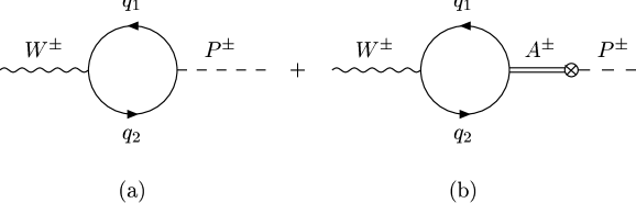
FIG. 2.: One–loop diagrams accounting for weak decays of pseudoscalar mesons.

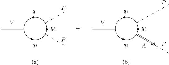
FIG. 3.: One–loop diagrams accounting for strong decays of vector mesons into two pseudoscalars.

FIG. 4.: One–loop diagrams accounting for anomalous decays of (a) pseudoscalars and (b) vector mesons

TABLE I.: Radiative decays of pseudoscalar and vector mesons. The second and third columns show the model predictions for different values of the ratio $F_{s}/F_{\pi}$ and the $\eta_{1}-\eta_{8}$ mixing angle $\theta_{P}$. The present experimental values for the decay rates are quoted in the last column.

Process	$\Gamma_{NJL}$ (KeV)				$\Gamma_{exp}$ (KeV)
	$F_{s}/F_{\pi}=2$	$F_{s}/F_{\pi}=1.75$	$F_{s}/F_{\pi}=1.75$	$F_{s}/F_{\pi}=1.4$
	$\theta_{P}=-10^{\circ}$	$\theta_{P}=-15^{\circ}$	$\theta_{P}=-20^{\circ}$	$\theta_{P}=-20^{\circ}$
$\pi^{0}\rightarrow\gamma\gamma$	$7.7\times 10^{-3}$	$7.7\times 10^{-3}$	$7.7\times 10^{-3}$	$7.7\times 10^{-3}$	$(7.7\pm 0.6)\times 10^{-3}$
$\eta\rightarrow\gamma\gamma$	0.53	0.63	0.76	0.71	$0.46\pm 0.04$
$\eta^{\prime}\rightarrow\gamma\gamma$	4.97	4.48	3.79	4.16	$4.28\pm 0.44$
$\eta^{\prime}\rightarrow\rho^{0}\gamma$	108	89.5	71.1	71.1	$59\pm 5$
$\eta^{\prime}\rightarrow\omega\gamma$	10.0	8.2	6.5	6.5	$6.1\pm 0.8$
$\rho^{0}\rightarrow\pi^{0}\gamma$	85	85	85	85	$102\pm 25$
$\omega\rightarrow\pi^{0}\gamma$	806	806	806	806	$720\pm 40$
$\rho^{0}\rightarrow\eta\gamma$	51	60	68	68	$36\pm 14$
$\omega\rightarrow\eta\gamma$	6.6	7.7	8.8	8.8	$5.5\pm 0.8$
$\phi\rightarrow\eta\gamma$	65.0	70.0	55.6	86.9	$57.8\pm 1.5$
$\phi\rightarrow\eta^{\prime}\gamma$	0.30	0.46	0.52	0.82	$0.30\pm 0.16$
${K^{\ast}}^{+}\rightarrow K^{+}\gamma$	62	62	62	62	$50\pm 5$
${K^{\ast}}^{0}\rightarrow K^{0}\gamma$	160	160	160	160	$117\pm 10$

REFERENCES

- [1] J. Gasser and H. Leutwyler, Ann. Phys. (N.Y.) 158, 142 (1984); Nucl. Phys. B250, 465 (1985).
- [2] Ö. Kaymakcalan, S. Rajeev and J. Scechter, Phys. Rev. D 30, 594 (1984); Ö. Kaymakcalan and J. Schechter, Phys. Rev. D 31, 1109 (1985); J. Schechter, Phys. Rev. D 34, 868 (1986).
- [3] H. Gomm, Ö. Kaymakcalan and J. Schechter, Phys. Rev. D 30, 2345 (1984); M. Spaliński, Z. Phys. C 42, 595 (1989).
- [4] G. Ecker, J. Gasser, A. Pich and E. de Rafael, Nucl. Phys. B321, 311 (1989).
- [5] J. Wess and B. Zumino, Phys. Lett. 37B, 95 (1971). E. Witten, Nucl. Phys. B223, 422 (1983).
- [6] Y. Nambú and G. Jona-Lasinio, Phys. Rev. 122, 345 (1961); 124, 246 (1961).
- [7] D. Ebert and H. Reinhardt, Nucl. Phys. B 271, 188 (1986); M. Wakamatsu and W. Weise, Z. Phys. A 331, 173 (1988).
- [8] T. Eguchi, Phys. Rev. D 14, 2755 (1976).
- [9] D. Ebert and M. Volkov, Z. Phys. C 16, 205 (1983).
- [10] M. Volkov, Ann. Phys. 157, 282 (1984).
- [11] D. Ebert, A. Ivanov and M. Volkov, Fortschr. Phys. 37, 487 (1989).
- [12] M. Volkov, Phys. Part. Nucl. 24, 35 (1993).
- [13] M. Jaminon, R. Méndez Galáin, G. Ripka and P. Strassart, Nucl. Phys. A 537, 418 (1992).
- [14] G. ’t Hooft, Phys. Rev. Lett. 37, 8 (1976).
- [15] S. P. Klevansky, Rev. Mod. Phys. 64, 649 (1992).
- [16] M. Wakamatsu, Ann. Phys. 193, 287 (1989).
- [17] A. Bramon, R. Escribano and M. Scadron, Eur. Phys. J. C 7, 271 (1999).
- [18] D. E. Groom et al., Eur. Phys. J. C 15, 1 (2000).
- [19] E. P. Venugopalan and B. R. Holstein, Phys. Rev. D 57, 4397 (1998).
- [20] T. Feldmann, Int. J. Mod. Phys. A 15, 159 (2000).