Extra Families, Higgs Spectrum and Oblique Corrections

Abstract

The standard model accommodates, but does not explain, three families of leptons and quarks, while various extensions suggest extra matter families. The oblique corrections from extra chiral families with relatively light (weak-scale) masses, $M_{f}\sim\langle H\rangle$, are analyzed and used to constrain the number of extra families and their spectrum. The analysis is motivated, in part, by recent $N=2$ supersymmetry constructions, but is performed in a model-independent way. It is shown that the correlations among the contributions to the three oblique parameters, rather than the contribution to a particular one, provide the most significant bound. Nevertheless, a single extra chiral family with a constrained spectrum is found to be consistent with precision data without requiring any other new physics source. Models with three additional families may also be accommodated but only by invoking additional new physics, most notably, a two-Higgs-doublet extension. The interplay between the spectra of the extra fermions and the Higgs boson(s) is analyzed in the case of either one or two Higgs doublets, and its implications are explored. In particular, the precision bound on the SM-like Higgs boson mass is shown to be significantly relaxed in the presence of an extra relatively light chiral family.

I Introduction

The number of fermion generations is one of the unresolved puzzles within the Standard Model (SM) of electroweak and strong interactions. However, certain extensions of the standard model suggest particular family structures.

$N=2$ supersymmetry constructions [1, 2], for instance, enforce an even number of generations, which in practice implies three additional mirror families of chiral fermions (and sfermions) with fermion masses at the weak scale, $M_{f}\sim\langle H\rangle$, where $\langle H\rangle\simeq 174$ GeV is the Higgs vacuum expectation value (VEV) responsible for the electroweak symmetry breaking. All fermion masses in $N=2$ supersymmetry originate at low-energy from effective Yukawa couplings, as shown in Ref. [2], and are chiral. (Although the matter fermions are vector-like in the $N=2$ limit, gauge invariant mass terms are forbidden by a $Z_{2}$ mirror parity [1, 2].) The mirror fermion spectrum is bounded from above by requiring perturbativity, and from below by direct collider searches. Hence, the natural mass range for the mirror fermions is roughly,

$$~{}\displaystyle\frac{m_{Z}}{2}~{}\lesssim~{}M_{f}~{}\lesssim~{}{\cal O}(\langle H\rangle)~{},$$ (1)

where $m_{Z}\simeq 91.19$ GeV is the mass of the weak gauge boson $Z^{0}$. Here, the generic lower bound is given by the LEP $Z$-decays to heavy neutrinos and other charged fermions. The current direct bound on charged heavy leptons is about $100$ GeV, while extra SM-like quarks $(t^{\prime},b^{\prime})$ should be heavier than $\sim\!100-200$ GeV, depending on detailed assumptions regarding their mixing with $(t,\,b)$ and their decay modes of $t^{\prime}\rightarrow b+W$ and $b^{\prime}\rightarrow b+Z$, etc [3]. For simplicity, we assume hereafter no mixing of the extra fermions among themselves and with the SM fermions (as the latter is suppressed by the mirror parity in $N=2$), and in particular, that the mass range (1) would apply.

Eq. (1) provides a restrictive range which is quite different from the case of dynamical symmetry breaking scenarios, such as technicolor, where the strongly interacting techni-fermions are generally heavy, with masses around or above the TeV scale [4, 5, 6]. The quantum oblique corrections, parameterized in terms of the $S$, $T$ and $U$ parameters [6], are extracted from the electroweak precision data [3, 7] and are known to exclude such extra heavy chiral-fermion generations [8]. For instance, one extra SM-like heavy family would contribute to the $S$-parameter by an amount of

$$\Delta S = \displaystyle\frac{1}{3\pi}\sum_{j}N_{cj}[I_{3L}(j)-I_{3R}(j)]^{2}=\frac{2}{3\pi}\simeq 0.21\,,$$ (2)

in the degenerate limit [6, 8], where $I_{3L,R}(j)$ is the third component of weak-isospin of the left (right) handed fermion $j$, and $N_{cj}=3\,(1)$ denotes the color number of quarks (leptons). On the other hand, a nondegenerate heavy fermion doublet $(\psi_{1},\,\psi_{2})$ with masses $(M_{1},M_{2})$ can yield a sizable positive $T$ which, in the limit $|M_{1}-M_{2}|\ll M_{1,2}$, reads [6, 9]

$$\Delta T \simeq \displaystyle\frac{N_{cj}}{12\pi s_{W}^{2}c_{W}^{2}}\left(\frac{M_{1}-M_{2}}{m_{Z}}\right)^{2}\,,$$ (3)

where $s_{W}=\sin\theta_{W}$ with $\theta_{W}$ being the weak angle. Such nondecoupling effects of heavy chiral fermions are due to the dependence of their masses on the Yukawa couplings, that necessarily violates the decoupling theorem [10]. The heavy (chiral) fermion corrections (2) and (3) are inconsistent with electroweak data (when considered separately), and are often the basis for ruling out such heavy fermion scenarios [8]. (This is contrary to the case of vector-like fermions whose contributions to all oblique parameters decouple as $1/M^{2}$ and which play a crucial role, for instance, in the recent top-quark seesaw models with either vector singlet [11] or doublet [12] heavy fermions.)

One expects models with relatively light extra chiral fermions to also receive non-trivial constraints from the electroweak quantum corrections, though the nature of the constraints may be very different. In this work, we study the oblique corrections from the such relatively light new fermions [cf. eq. (1)], as well as from the Higgs sector which generates the chiral fermion masses. Since the extra fermions under consideration are relatively light, they can have a sizable mass-splitting, such as $|M_{1}-M_{2}|\sim m_{Z}\not\ll M_{1,2}$, without causing an unacceptably large $T$. At the same time, the $S$-parameter may receive additional negative corrections. Interestingly, a single relatively heavy SM Higgs boson leads to a sizable negative contribution to $T$, and thus allows for a larger isospin breaking in the fermion sector. For one extra fermion family with a proper spectrum, a SM Higgs boson as heavy as 500 GeV is found to be consistent with the precision electroweak data. Such an interplay is nontrivial, and as we will show, in order to accommodate up to three new families, an extended Higgs sector with two Higgs doublets (and with a highly constrained spectrum) has to be considered.

We begin, in Sec. II, with a summary of the definitions of the oblique parameters ${(S,T,U)}$ and their current experimental bounds, and examine in detail the contributions in the extra lepton-quark sector and the two-Higgs-doublet sector. We study the interplay between the fermion and Higgs sectors in Sec. III, where ${(S,T,U)}$ bounds are imposed for deriving the allowed parameter space. This is done first in the simplest case with a single extra fermion family and the one Higgs doublet, and then in the case with three extra fermion families and the two Higgs doublets. Low energy $N=2$ supersymmetry, which provides an explicit theoretical framework in the latter case, is briefly reviewed as well. We conclude in Sec. IV. The Appendix summarizes the complete formulae for the two-Higgs-doublet contributions to ${(S,T,U)}$.

II New Physics Corrections to Oblique Parameters

A The Oblique Parameters and Current Bounds

The oblique ${(S,T,U)}$ parameters [6] can be defined as

$$S = -16\pi\frac{\Pi_{3Y}(m_{Z}^{2})-\Pi_{3Y}(0)}{m_{Z}^{2}}\,,$$ (4)

$$T = 4\pi\frac{\Pi_{11}(0)-\Pi_{33}(0)}{s_{W}^{2}c_{W}^{2}m_{Z}^{2}}\,,$$ (5)

$$U = 16\pi\frac{[\Pi_{11}(m_{Z}^{2})-\Pi_{11}(0)]-[\Pi_{33}(m_{Z}^{2})-\Pi_{33}(0)]}{m_{Z}^{2}}\,,$$ (6)

where the weak-mixing angle $\theta_{W}$ is defined at the scale $\mu=m_{Z}$. In eqs. (4)-(6), $\Pi_{11}$ and $\Pi_{33}$ are the vacuum polarizations of isospin currents, and $\Pi_{3Y}$ the vacuum polarization of one isospin and one hypercharge currents. The above definitions slightly differ from the original ones [6] for $(S,U)$ since we use the differences of $\Pi$-functions rather than their first derivatives (with higher powers of $q^{2}=m_{Z}^{2}$ truncated). Eqs. (4)-(6) are more appropriate for our current analysis in which the scale of the relevant new fermions is relatively low. The new physics corrections to ${(S,T,U)}$ are defined relative to their SM reference point and are often denoted by $(S_{\rm new},\,T_{\rm new},\,U_{\rm new})$. To simplify the notation, we will omit these subscripts hereafter.

In certain cases, three additional oblique parameters $(V,\,W,\,X)$ [13], which are generally less visible, may be further included in fitting the data. This more elaborated procedure is beyond the scope of the current work and is not expected to affect our main conclusions. [The contributions of the new fermions to $(V,\,W,\,X)$ drop quickly as their masses increase beyond the $Z$-pole and become well below the dominant oblique corections [13].] Also, the absence of mixings between new fermions and the SM fermions implies no extra flavor-dependent vertex corrections to the fermionic $Z$-decay width, which makes the oblique corrections sufficient for describing the new physics in our case.

The updated global fit of ${(S,T,U)}$ to the various precisely measured electroweak observables (such as the gauge boson masses $(m_{Z},m_{W})$, the $Z$-width $\Gamma_{Z}$, and the $Z$-pole asymmetries, etc) [3, 7] gives:

$$S = -0.04\pm{0.11}\,(-0.09)\,,$$ (7)

$$T = -0.03\pm{0.13}\,(+0.09)\,,$$ (8)

$$U = \ \ \,0.18\pm{0.14}\,(+0.01)\,,$$ (9)

where the central values correspond to the SM Higgs mass reference point, ${m_{H}^{\rm sm}}=100$ GeV, while the values given in the parentheses show the changes for ${m_{H}^{\rm sm}}=300$ GeV. The uncertainties in (8) are from the inputs. The $S$ and $T$ parameters are strongly correlated as shown in the $95\%$ C.L. contours of Fig. 1. Variations in $U$ mainly shift the $S-T$ contour without affecting its shape and direction, and a larger positive $U$ tends to diminish the allowed regions of positive $(S,\,T)$.

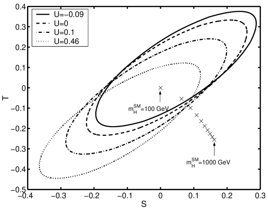
FIG. 1.: The ${95\%\,{\rm C.L.}}$ contours for $S$ and $T$ for fixed values of $U$ (within 2$\sigma$ range) and the reference point ${m_{H}^{\rm sm}}=100$ GeV. The “$\times$” symbols denote the SM Higgs contributions to $(S,\,T)$ for ${m_{H}^{\rm sm}}=100,\,200,\,\dots,\,1000$ GeV (from left to right) relative to the reference point (the origin of the $S-T$ plane).

The “$\times$” symbols in Fig. 1 represent in SM Higgs contributions to $S$ and $T$ for different ${m_{H}^{\rm sm}}$ values relative to ${m_{H}^{\rm sm}}=100$ GeV. $U$ is insensitive to ${m_{H}^{\rm sm}}$ for ${m_{H}^{\rm sm}}\gtrsim 200$ GeV. An important feature of the SM Higgs corrections is that as ${m_{H}^{\rm sm}}$ increases, $S$ becomes more positive while $T$ is driven to more negative values. As such, a SM Higgs with a mass ${m_{H}^{\rm sm}}\gtrsim 300$ GeV is clearly outside the $95\%$ C.L. $S-T$ contours for wide range of $U$ values. However, including certain types of new physics contributions to ${(S,T,U)}$ may drastically relax the upper bound on the Higgs mass, as long as the new corrections either (i) decrease $S$, or (ii) lift up $T$, or (iii) achieve both. As we will show in the following sections, the extra fermions under consideration generally lead to a large positive $T$, and in many cases also to a sizable $S>0$. Hence, our analysis will mainly fall under Case (ii).

B Lepton and Quark Sector

For generality, we consider two fermions $(\psi_{1},\psi_{2})$, with masses $(M_{1},M_{2})$ and the following SM charges,

$$\begin{array}[]{lccc}{\rm Fermions:}&\displaystyle\psi_{L}=\left(\begin{array}[]{c}\psi_{1L}\\ \psi_{2L}\end{array}\right)\,,{}{}{}{}&\psi_{1R}\,,{}{}{}{}&\psi_{2R}\,;\\[8.53581pt] {\rm Hypercharge:}&Y\,,{}{}{}{}&\displaystyle Y+\frac{1}{2},{}{}{}{}&\displaystyle Y-\frac{1}{2};\end{array}$$ (10)

where the electric charge is given by $Q_{j}=I_{3j}+Y_{j}$ with $I_{3j}$ and $Y_{j}$ being the third component of weak-isospin and the hypercharge of the fermion $j$, respectively. For SM fermions, one has $Y=\frac{1}{6}\,\left(-\frac{1}{2}\right)$ in eq. (10) for quarks (leptons). For mirror fermions in the Minimal $N=2$ Supersymmetric SM (MN2SSM) [2], one has $Y=-\frac{1}{6}\,\left(\frac{1}{2}\right)$ in eq. (10) for mirror quarks (mirror leptons). (For a review on the MN2SSM, see Sec. III B.) Hence, the correspondence with eq. (10) is, $(M_{1},M_{2})\leftrightarrow{(M_{\nu},M_{\ell})}$ for leptons and $(M_{1},M_{2})\leftrightarrow{(M_{\ell^{\prime}},M_{{\nu}^{\prime}})}$ for mirror leptons, and similarly for the quarks and mirror quarks.

Using eqs. (4)-(6), we can compute the one-loop fermionic contributions to the oblique ${(S,T,U)}$ parameters as below,

$$S_{f} = \frac{N_{c}}{6\pi}\left\{2(4Y+3)x_{1}+2(-4Y+3)x_{2}-2Y\ln\frac{x_{1}}{x_{2}}\right.$$ (12)

$$\left.+\left[\left(\frac{3}{2}+2Y\right)x_{1}+Y\right]G(x_{1})+\left[\left(\frac{3}{2}-2Y\right)x_{2}-Y\right]G(x_{2})\right\}\,,$$

$$T_{f} = \frac{N_{c}}{8\pi{s}_{W}^{2}c_{W}^{2}}F(x_{1},x_{2})\,,$$ (13)

$$U_{f} = -\frac{N_{c}}{2\pi}\left\{\frac{x_{1}+x_{2}}{2}-\frac{(x_{1}-x_{2})^{2}}{3}+\left[\frac{(x_{1}-x_{2})^{3}}{6}-\frac{1}{2}\,\frac{x_{1}^{2}+x_{2}^{2}}{x_{1}-x_{2}}\right]\ln\frac{x_{1}}{x_{2}}\right.$$ (15)

$$+\left.\frac{x_{1}-1}{6}f(x_{1},x_{1})+\frac{x_{2}-1}{6}f(x_{2},x_{2})+\left[\frac{1}{3}-\frac{x_{1}+x_{2}}{6}-\frac{(x_{1}-x_{2})^{2}}{6}\right]f(x_{1},x_{2})\right\},$$

where $x_{i}=(M_{i}/m_{Z})^{2}$ with $i=1,2$ and the color factor $N_{c}=3\,(1)$ for quarks (leptons). The functions $G(x)$, $F(x_{1},x_{2})$, and $f(x_{1},x_{2})$ are defined by eqs. (A21), (A20) and (A25), in the Appendix. We observe that for a given $(M_{1},\,M_{2})$, eq. (12) is invariant under the exchanges of $Y\leftrightarrow{-}Y$ and $M_{1}\leftrightarrow{M}_{2}$, so that the fermions $(\psi_{1},\,\psi_{2})$ and their mirrors $(\psi_{2},\,\psi_{1})$ have the same expression for $S$. Therefore, we will not distinguish hereafter between a fermion and its mirror, but simply use $(M_{1},\,M_{2})$ to denote $(M_{N},\,M_{E})$ in the (mirror) lepton sector and $(M_{U},\,M_{D})$ in the (mirror) quark sector.

It is instructive to consider the limit $M_{1,2}^{2}\gg{m_{Z}^{2}}$, under which the $S$ parameter approximately reads,

$$S_{f}=\frac{N_{c}}{6\pi}\left[1-2Y\ln\left(\frac{M_{1}}{M_{2}}\right)^{2}+\frac{1+8Y}{20}\left(\frac{m_{Z}}{M_{1}}\right)^{2}+\frac{1-8Y}{20}\left(\frac{m_{Z}}{M_{2}}\right)^{2}+O\left(\frac{m_{Z}^{4}}{M_{i}^{4}}\right)\right].$$ (16)

If the mass splitting  $|M_{1}-M_{2}|/M_{1,2}$  is small, then all mass-dependent terms decouple and eq. (16) reduces to the positive constant term $N_{c}/6\pi$, which leads to the well-known result in eq. (2). However, as long as $(M_{1},\,M_{2})$ are non-degenerate and not too large, additional negative corrections to the constant term $N_{c}/6\pi$ may arise, depending on the sign of hypercharge $Y$.

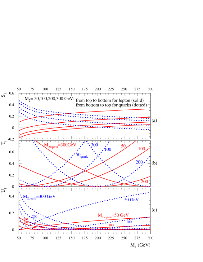
FIG. 2.: The contributions to $S$, $T$ and $U$ from one extra family of leptons (solid curves) and quarks (dotted curves).

The contributions to $S$ from one generation of either ordinary or mirror leptons and quarks are shown in Fig. 2(a), where the solid curves are for leptons and dotted curves for quarks. The mass range of the chiral fermions are chosen to be between 50 GeV and 300 GeV. (We note that after adding experimental bounds on the charged extra fermions, the lower end of their mass range would be shifted somewhat above $50$ GeV, depending on the details of each particular model.) The lepton contribution to $S$ grows with an increasing $M_{1}$ ($M_{N}$) and with a decreasing $M_{2}$ ($M_{E}$), while the quark contribution behaves in the opposite way. This is due to their different signs of $Y$. The quark contribution is enhanced by the color factor, but is suppressed by the smaller Y. For $M_{1,2}^{2}\gg{m}_{Z}^{2},(M_{1}-M_{2})^{2}$, $S$ should approach its asymptotic value $1/6\pi$ for leptons and $1/2\pi$ for quarks. This may be understood from Fig. 2(a) by examining the solid (dotted) curve with $M_{2}=300$ GeV which already well approaches $\sim\!0.05~{}(0.16)$ for leptons (quarks) as $M_{1}$ increases to about $300$ GeV. However, for quarks and leptons with masses $\sim{\cal O}(m_{Z})$, smaller and even negative values of $S$ can be obtained. Negative values of $S$ occur in the non-degenerate region of $M_{E}>M_{N}$ and $M_{U}>M_{D}$. For instance, $(M_{N},\,M_{E})=(50,\,300)$ GeV gives $S_{\ell}=-0.18$.

The contributions to $T$ and $U$ from chiral fermions are depicted in Fig. 2(b) and (c). The parameters $T$ and $U$ measure the weak-isospin violation in the ${\rm SU}(2)_{L}$ doublet and thus are nonvanishing only for $M_{1}\neq M_{2}$. The more $M_{1}$ and $M_{2}$ split, the larger their contributions to $(T_{f},\,U_{f})$ become. Furthermore, the $(T_{f},\,U_{f})$ formulae eqs. (13) and (15) are invariant under the exchange $M_{1}\leftrightarrow{M}_{2}$ and are always positive, unlike the contributions of the Higgs boson (cf., Fig. 1). While ${U}_{f}$ is relatively small, ${T}_{\ell}$, for example, could be as large as 0.68 for $(M_{N},\,M_{E})=(100,300)$ GeV. Since $(T_{f},\,U_{f})$ depend only on isospin-breaking and are symmetric under $M_{1}\leftrightarrow M_{2}$, their $M_{1,2}$-dependence is the same for fermions and mirror fermions. The quark contributions to $(T_{f},\,U_{f})$ are again enhanced by their color factor.

In order to accommodate new fermion families, the up- and down-type (mirror) quarks have to be sufficiently degenerate to avoid a too large positive $T$. Unfortunately, this renders $S$ positive in most of the parameter space. A non-degenerate pair of (mirror) leptons could help to satisfy the $S$ constraint, but it also contributes positively to $T$ (though more moderately comparing to quark). A positive contribution to $U$ can better fit the data, but it is numerically less significant, as shown in Fig. 2(c). Clearly, the nontrivial correlations among lepton and quark contributions to all three oblique parameters (rather than to any particular one) provide the most significant constraints.

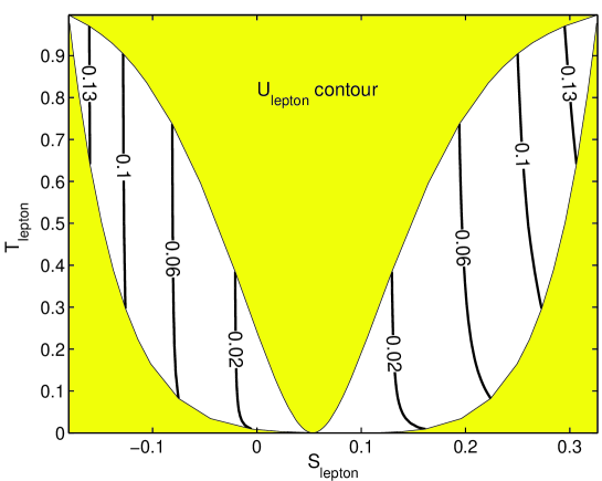
FIG. 3.: $U$ contours in the $S-T$ plane for one generation of (mirror) leptons, which are derived from eqs. (12)-(15) for the mass range $50\leq m_{\ell}\leq 300$ GeV and with no experimental bounds imposed. The shaded areas cannot be theoretically reached.

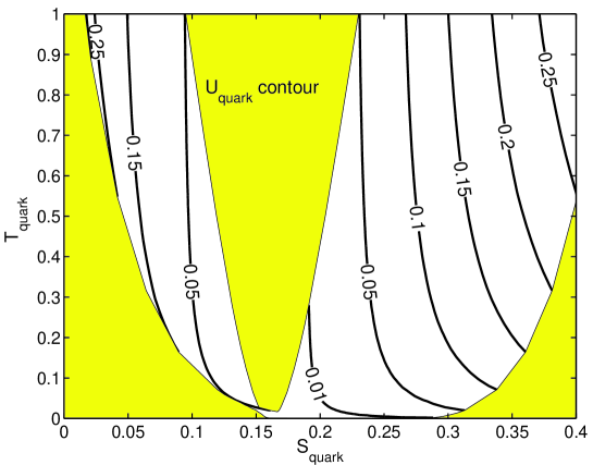
FIG. 4.: $U$ contours in the $S-T$ plane for one generation of (mirror) quarks, which are derived from eqs. (12)-(15) for the mass range $50\leq m_{q}\leq 300$ GeV and with no experimental bounds imposed. The shaded areas cannot be theoretically reached.

In order to compare the theoretical predictions with the current experimental constraints shown in Fig. 1, it is very instructive to depict the above fermionic oblique corrections eqs. (12)-(15) in the $S-T$ plane for given values of $U$. This corresponds to a set of “$U$-contours” in the theoretically allowed regions of the $S-T$ plane, which should be directly compared to the experimental bounds of Fig. 1. In Figs. 3 and 4, we plot various $U$-contours in the $S-T$ plane for one family of leptons and of quarks, respectively. For leptons, $S_{\ell}$ can be negative in large regions of the parameter space. For quarks, $S_{q}>0$ in most of the parameter space as to avoid a too large contribution to $T_{q}$. Although a positive $U_{f}$ is consistent with the data, $T_{f}$ provides a very strong constraint when combined with $S_{f}$. Nevertheless, comparing with the $S-T$ fits in Fig. 1, one finds that one extra chiral family is viable, even without additional new physics contributions. This is consistent with the recent study in Ref. [16], where a similar conclusion was reached. Ref. [16] used an unconventional formalism for analyzing the oblique corrections and a detailed comparison is difficult. Our analysis, based on the standard ${(S,T,U)}$ formalism [6], is transparent and can be readily applied to a given model. In what follows, we focus on the interplay between extra families and the Higgs sector. We aim at accommodating up to three chiral families (as theoretically motivated by our recent $N=2$ constructions [2]), which requires to extend the Higgs sector with two-doublets. Henceforth, our study substantially differs from Ref. [16].

Finally, we note that it should be straightforward to translate above Figs. 3 and 4 to any number $N_{g}$ of extra generations, i.e., for $N_{g}>1$, the same curves represent the oblique parameters with the values ${(S,T,U)}/N_{g}$, if one assumes that these new generations are degenerate in mass with each other. However, it is extremely difficult to accommodate more than one extra generation with the data. We will return to this issue in Sec. III.

C Two Higgs Doublet sector

The exact corrections to ${(S,T,U)}$ in a general two-Higgs-doublet model (2HDM) have been computed in Ref. [17]. We will denote these contributions by $S_{H}$, $T_{H}$, and $U_{H}$, respectively. Their explicit formulae are lengthy and are summarized in the Appendix for completeness. For $N=1$ supersymmetry, and in particular the $N=1$ minimal supersymmetric extension of the SM (MSSM) (with high-scale supersymmetry breaking), the Higgs contributions are generally small due to the tree-level constraints among the masses of the light and heavy CP-even, the CP-odd, and the charged Higgs bosons, ($m_{h},\,m_{H},\,m_{A},\,m_{H^{\pm}}$, respectively). However, for a two-Higgs-doublet sector with a general Higgs mass spectrum, significant contributions can arise in large regions of the parameter space. Such non-MSSM-like Higgs spectrum may be realized for a $N=1$ or $N=2$ supersymmetry scenario with a sufficiently low scale of supersymmetry breaking [18].

The contribution $T_{H}$ could be either positive or negative, depending on the spectrum of the Higgs masses and on the difference between the two rotation angles ($\beta-\alpha$), where $\tan\beta=\langle H_{2}\rangle/\langle H_{1}\rangle$ [with $H_{1}$ ($H_{2}$) being the Higgs doublet of negative (positive) hypercharge] and $\alpha$ is the rotation angle for obtaining the CP-even mass-eigenstates $(h^{0},\,H^{0})$. The $T$-contours in the $(m_{h},m_{H})$ plane for $m_{A}=1000$ GeV and $m_{A}=100$ GeV are shown in Figs. 5 and 6 for $\beta-\alpha=\pi$ (solid line), $\frac{3\pi}{4}$ (dash-dotted line) and $\frac{\pi}{2}$ (dotted line), where $m_{H^{\pm}}$ is chosen as to minimize $T_{H}$.

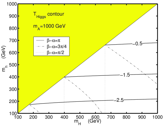
FIG. 5.: Contours for $T_{H}$ in the 2HDM for $m_{A}=1000$ GeV and $\beta-\alpha=\pi$ (solid line), $\frac{3\pi}{4}$ (dash-dotted line) and $\frac{\pi}{2}$ (dotted line). Here we consider $\tan\beta>1$ ($\frac{\pi}{4}<\beta<\frac{\pi}{2}$) and $-\frac{\pi}{2}<\alpha<0$, so that $\frac{\pi}{4}<\beta-\alpha<\pi$. The $m_{H^{\pm}}$ value is chosen to minimize $T_{H}$. These contours are derived from eq. (A6).

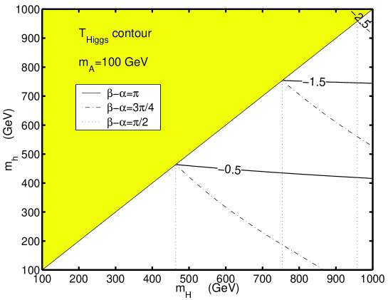
FIG. 6.: Contours for $T_{H}$ in the 2HDM for $m_{A}=100$ GeV. Notation is the same as in Fig. 5.

A negative contribution to $T_{H}$ can always be achieved with an appropriately chosen $m_{H^{\pm}}$. (This was also noted in Ref. [19].) For some values of $m_{H^{\pm}}$, $T_{H}$ could be positive and large, however, we will concentrate hereafter only on the more interesting regions with negative $T_{H}$.

The regions which correspond to a sizable negative $T_{H}$ can be classified as follows:

• Large $m_{A}$: (Ia) $m_{h}\ll m_{H^{\pm}}\ll{m}_{A}$,  $\beta-\alpha\sim\pi$ ;
                    (Ib) $m_{h}\sim{m}_{H}\ll m_{H^{\pm}}\ll{m}_{A}$ ;

• Small $m_{A}$: (IIa) $m_{A}\ll{m}_{H^{\pm}}\ll m_{H}$,  $\displaystyle\beta-\alpha\sim\frac{\pi}{2}$ ;
                    (IIb) $m_{A}\ll{m}_{H^{\pm}}\ll m_{h}\sim{m}_{H}$ ;

where the minimum value for $T_{H}$ is achieved for $m_{H^{\pm}}\simeq{0.6}\ m_{\rm heavy}$ and $m_{\rm heavy}=\max(m_{H},\,m_{A})$. This can be understood by examining the approximate formula for $T_{H}$ in the limit $m_{\rm Higgs}^{2}\gg{m_{Z}}^{2}$ [19]:

$$T_{H} = \frac{1}{16\pi{s}^{2}_{W}m^{2}_{W}}\left\{\cos^{2}({\beta-\alpha})\left[F(m_{H^{\pm}}^{2},m_{h}^{2})+F(m_{H^{\pm}}^{2},m_{A}^{2},)-F(m_{A}^{2},m_{h}^{2},)\right]\right.$$ (18)

$$\hskip 54.91382pt+\left.\sin^{2}({\beta-\alpha})\left[F(m_{H^{\pm}}^{2},m_{H}^{2})+F(m_{H^{\pm}}^{2},m_{A}^{2})-F(m_{A}^{2},m_{H}^{2})\right]\right\},$$

where $F(x_{1},x_{2})$ is defined in eq. (A20). [The approximate formulae for ($S_{H},\,U_{H}$) are given in the Appendix for completeness.] Terms inside the first (second) bracket are symmetric in $m_{h(H)}$ and $m_{A}$, and could obtain large negative values if there is a large split between $m_{h(H)}$ and $m_{A}$ and $m_{\rm light}\ll{m}_{H^{\pm}}\ll{m}_{\rm heavy}$. For $\beta-\alpha=\pi\,[{\pi\over 2}]$, we have $\sin^{2}({\alpha-\beta})=0\,[\cos^{2}({\alpha-\beta})=0]$, so that only the first (second) bracket contributes, which is independent of $m_{H}$ ($m_{h}$). This is the case in region (Ia) and (IIa). For general values of $\beta-\alpha$, $m_{h}$ and $m_{H}$ have to be sufficiently close in order for $T_{H}$ to be large and negative. This is the case in regions (Ib) and (IIb). We also notice that in Figs. 5 and 6, each set of $T_{H}$-contours approach the same point at the boundary of $m_{h}=m_{H}$. This is because the dependence on $\beta-\alpha$ disappears under this limit [see eqs. (A6) and (18)].

We note that the parameter $T_{H}$ can be as negative as $-2.5$, and could cancel large positive contributions from the quark and lepton sector when more than one extra family is included. $S_{H}$ and $U_{H}$ are relatively small in these two regions, where one has an almost positive $S_{H}<0.1$ and a negative $U_{H}$ with $|U_{H}|<0.02$. In Case-(Ia), a sizable positive $S_{H}\sim{0.16}$ and a slightly negative $U_{H}\sim{-0.05}$ are also possible.

Clearly, the Higgs spectrum in these two regions is very different from that of the conventional $N=1$ MSSM. Even in the case of a more general supersymmetry breaking scenario [18], it requires some fine-tuning of the mass parameters and the quartic couplings. In principle, such relations are easier to realize in models with more than two Higgs doublets (such as $N=2$ supersymmetry), where more Higgs states can exist at the scale $m_{\rm heavy}$ or above and thus considerably expand the parameter space.

The correlations between the spectra of the minimal one- or two-Higgs-doublet sector and the additional chiral families via the precision ${(S,T,U)}$ constraints will be systematically analyzed in the next section.

D Other Super and Mirror Particles

The contributions of the $N=1$ sparticles, with a typical mass scale $M_{\rm SUSY}$, to the oblique parameters are generally small in the decoupling region $M_{\rm SUSY}\gg{m}_{Z},m_{t}$, which we will assume in our analysis for simplicity. In practice, this only requires $M_{\rm SUSY}\gtrsim 300$ GeV, as shown in Refs. [17, 20, 21]. Aside from sfermions and mirror sfermions, there could also be visible contributions from Majorana fermions, such as gauginos, Higgsinos, and, in $N=2$, mirror gauginos and Higgsinos. In general, contributions from Majorana fermions to $S$ could have either sign [16, 22].

In our current study we concentrate on the contributions of the Higgs bosons and of (mirror) quarks and leptons. For simplicity, the effects from sfermions and Majorana fermions are assumed to be negligible. This is indeed the case in the decoupling regime $M_{\rm SUSY}\gg{m}_{Z},m_{t}$ under consideration. Clearly, an arbitrary spectrum of sparticles and/or mirror gauginos will add more degrees of freedom to fit the data and thus further relax the correlations derived in the next section. A more elaborate analysis including these complications is left for future work.

III Spectra of Extra Fermions and Higgs Bosons:
The Interplay

A Interplay of Extra Fermions and One-Higgs-Doublet Sector

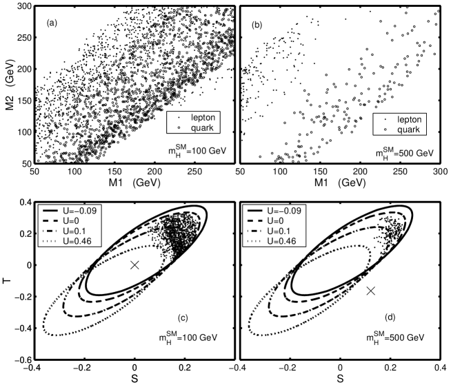
FIG. 7.: The $M_{1}-M_{2}$ plane is scanned assuming one extra family of leptons (dots) and of quarks (circles) and one Higgs doublet. The allowed region is defined by the models which are admitted by the data. Figure (a) is shown for ${m_{H}^{\rm sm}}=100$ GeV and Figure (b) for ${m_{H}^{\rm sm}}=500$ GeV. In Figures (c) and (d), the allowed points are shown in the $S-T$ plane (with the ${95\%\,{\rm C.L.}}$ experimental bounds displayed for comparison) for ${m_{H}^{\rm sm}}=100$ GeV and 500 GeV, respectively, and the “$\times$” symbols denote the corresponding SM Higgs contributions.

We begin by considering the simplest case with one extra (mirror) family and one (SM) Higgs doublet. We display in Fig. 7 (a) and (b), the $M_{1}-M_{2}$ plane, where each point represents an experimentally viable four-generation model, and dots and circles represent leptons and quarks, respectively. The initial sample consists of 10000 models. We choose, for illustration, a light SM Higgs with mass ${m_{H}^{\rm sm}}=100$ GeV [cf., Fig. 7(a)] and a heavy SM Higgs with mass ${m_{H}^{\rm sm}}=500$ GeV [cf., Fig. 7(b)]. Large regions of the parameter space are allowed, where the preferred regions are given by $M_{2}>M_{1}$ for leptons and $M_{1}>M_{2}$ for quarks. For a heavy Higgs boson ${m_{H}^{\rm sm}}=500$ GeV, the leptons and quarks occupy different mass regions, while in the case of a very light Higgs boson they largely overlap. Future discoveries of light extra lepton/quark spectra can provide important information about the Higgs boson mass range, and vice versa. Figs. 7(c) and (d) display the corresponding points in the $S-T$ plane with the ${95\%\,{\rm C.L.}}$ experimental bounds superimposed for ${m_{H}^{\rm sm}}=100$ GeV and 500 GeV, respectively. From Fig. 7(d), we see that for one extra chiral family, a heavy SM Higgs with ${m_{H}^{\rm sm}}=500$ GeV can be accommodated via the scenario of large fermionic $T_{f}>0$.

We note in passing that, after the completion of this work, Ref. [23] analyzed the limits on a heavy SM Higgs boson in the case of TeV-scale heavy technifermions which generate a large positive contribution to $T$. Our study has solely focused on relatively light extra chiral families with masses significantly below ${\cal O}({\rm TeV})$, as motivated by $N=2$ supersymmetry constructions [1, 2]. The relaxation of the Higgs mass limits derived from precision electroweak data could be significant in either case.

B Minimal $N=2$ Supersymmetric SM and Mirror Families

Before proceeding to discuss the case with three extra chiral families and the two-Higgs-doublets, a review of the theoretical framework which motivates this scenario is in place. As mentioned earlier, this spectrum arises in constructions of low-energy $N=2$ supersymmetry. Low-energy realizations of $N=2$ supersymmetry and its related phenomenology were recently investigated in Ref. [2]. In the minimal $N=2$ supersymmetric SM, for each of the ordinary quark (lepton) and its squark (slepton) superpartner of the $N=1$ extension, there is also a conjugate mirror quark (mirror lepton) and its mirror squark (mirror slepton) superpartner. For each gauge boson and gaugino, there is also a mirror gauge boson and a mirror gaugino. The Higgs and Higgsino are also accompanied by their mirrors. In particular, three additional mirror generations of chiral fermions are predicted in the MN2SSM.

The mirror quarks and leptons do not obtain gauge-invariant vectorial mass terms (which would mix the mirror and ordinary sectors) due to a $Z_{2}$ mirror parity [2]. Instead, their masses arise from effective Yukawa interactions and are thus proportional to the relevant Higgs VEVs of electroweak symmetry breaking (EWSB). As such, their mass range is constrained to be at the weak scale [cf., eq. (1)]. In order to realize ${\cal O}(1)$ effective Yukawa couplings at low energies, supersymmetry itself is broken at a low scale. The large Yukawa couplings also imply that mirror fermion/sfermion loops can significantly modify the CP-even Higgs spectrum at one loop. (This is similar to the usual top/stop sector, but now all three mirror families may contribute).

The MN2SSM Higgs sector is less constrained than that of the MSSM or other $N=1$ frameworks. In particular, any one of the four Higgs doublets which appear in MN2SSM [2] could participate in EWSB. Even when assuming for simplicity a MSSM-like Higgs structure with two-doublets participating in the EWSB, the $N=2$ two-Higgs-doublet spectrum could be quite different from that of the MSSM. This is because the tree-level Higgs quartic couplings $\lambda$ arise not only from supersymmetric terms $\lambda\sim g^{2}$, for $g$ being the gauge coupling, as in the MSSM, but also from hard supersymmetry breaking operators (whose generation goes hand in hand with that of the effective Yukawa couplings) $\lambda_{i}\sim(g^{2})+\kappa_{i}$ [18], where $\kappa_{i}$ is the contribution from higher order operators in the Kähler potential. Therefore, the usual MSSM relations among the Higgs mass eigenvalues $m_{h}\ll{m}_{H}\sim{m}_{A}\sim{m}_{H^{\pm}}$ (assuming $m_{A}\gg{m}_{Z}$) no longer hold, and the physical Higgs mass spectrum is somewhat arbitrary. This observation is generic to any theory with low-energy supersymmetry breaking where $\kappa\sim{\cal{O}}(1)$ is realized [18].

We note in passing that models with higher dimensions often lead after compactification to an effective $N=2$ structure in four-dimensions. Therefore, our analysis of $N=2$ models and of the associated mirror families may be applied in certain cases to theories with large extra dimensions.

C Interplay of Extra Fermions and Two-Higgs-Doublet Sector

It was shown above that one extra chiral generation ($N_{g}=1$) can be accommodated by the precision data with the SM Higgs mass up to about $500$ GeV. This is not the case for $N_{g}=2$ and $N_{g}=3$. In fact, the $N_{g}=3$ case, as predicted in the MN2SSM, requires additional new physics contributions (beyond that of a single Higgs doublet) to the oblique parameters. The minimal version of such an extension is to invoke the two-Higgs-doublet sector. For generality (and being consistent with the $N=2$ framework described above), we will consider a general 2HDM. Thus, our analysis is valid for any given model which contains two Higgs doublets together with extra families, and our constraints on the parameter space can be readily applied to any such model.

The two-Higgs-doublet sector can lead to a large negative $T_{H}$ (cf. Sec. II C) which will cancel to a large part the three-family fermionic $T_{f}$, and render the sum $T=T_{f}+T_{H}$ consistent with the experimental bounds over certain regions of the parameter space. For simplicity, we will assume the second and third families to have the same mass spectrum as the first family. This interplay is explored in Fig. 8, which is based on an initial sample of 50000 models. Allowed models are determined by imposing the ${95\%\,{\rm C.L.}}$ bounds of ${(S,T,U)}$. Figs. 8(a) and (b) display the extra fermions and the Higgs bosons spectra, respectively. We choose, for illustration, a typical set of Higgs inputs $(m_{h},\,m_{H},\,m_{A},\,m_{H^{\pm}})=(115,\,120,\,1000,\,580)$ GeV and $\beta-\alpha=3\pi/4$ in (a), and a set of fermionic inputs $(M_{N},\,M_{E})=(60,\,250)$ GeV, $(M_{U},\,M_{D})=(250,\,200)$ GeV in (b), where three values of $\beta-\alpha$ are shown. Figs. 8(c) and (d) display the allowed points, with the same inputs as (a) and (b), respectively, in the $S-T$ plane for comparison with the experimental bounds. Variation of $m_{h}=115$ GeV in the $\sim\!100-200$ GeV range does not change the results. Also, for clarity, only $\beta-\alpha=\pi$ is shown in (d), but similar results are obtained for the case of $\beta-\alpha=\pi/2$, or, $3\pi/4$.

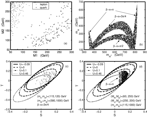
FIG. 8.: The allowed parameter space for the scenario with three extra families and the two Higgs doublets is shown, (a) in the $M_{1}-M_{2}$ plane for $(m_{h},\,m_{H},\,m_{A},\,m_{H^{\pm}})=$ $(115,\,120,\,1000,\,580)$ GeV and $\beta-\alpha=3\pi/4$ [where dots (circles) denote leptons (quarks)]; (b) in the Higgs mass plane for $(M_{N},\,M_{E})=(60,\,250)$ GeV, $(M_{U},\,M_{D})=(250,\,200)$ GeV, and for three values of $\beta-\alpha$. In (c) and (d), the allowed points are shown in the $S-T$ plane (with the ${95\%\,{\rm C.L.}}$ experimental bounds displayed), corresponding to the inputs of (a) and (b), respectively. For (d), only $\beta-\alpha=\pi$ is chosen for the illustration.

The choice of the above Higgs inputs in Figs. 8(a) and (c) corresponds to a small allowed region in the $M_{1}-M_{2}$ plane, i.e., the mirror leptons (dots) are highly non-degenerate, while the mirror quarks (circles) exhibit much smaller isospin breaking. Similar results could be obtained for other choices of Higgs masses, where the Higgs contribution $T_{H}$ is sizable and negative. From Fig. 8(b), one observes that the allowed regions are quite distinct for three choices of $\beta-\alpha\in(\pi/2,\,3\pi/4,\,\pi)$. For $\beta-\alpha=\pi$, $m_{H}$ could vary in a wide range [corresponding to case (Ia)] for $m_{H^{\pm}}\sim 800$ GeV. In all other cases, the heavier neutral Higgs $H^{0}$ has to be generally much lighter than 1 TeV. It is interesting to note that for $m_{H^{0}}\lesssim 200$ GeV (i.e., slightly heavier than $h^{0}$), the charged Higgs mass $m_{H^{\pm}}$ is confined into two very narrow regions around either $350-450$ GeV or $750-800$ GeV, for a sizable range of $\beta-\alpha$. Finally, Figs. 8(c) and (d) indicate that the relevant viable parameter space typically corresponds to $0\lesssim S\lesssim 0.2$ and $-0.1\lesssim T\lesssim 0.2$. In comparison with the scenario of one-generation and one-Higgs-doublet [cf., Fig. 7(c)-(d)], the viable region in the $S-T$ plane of Fig. 8(c)-(d) has a smaller $T=T_{f}+T_{H}$. This is due to the more negative $T_{H}$ values contributed by the two-Higgs-doublet sector.

Clearly, there are strong correlations among the allowed Higgs and the fermion mass ranges in the $N_{g}=3$ scenario. This renders the model highly restrictive in its parameter space, and it is thus instructive and encouraging for the relevant experimental tests at the upcoming colliders, such as the Tevatron Run-II, the LHC and the future lepton colliders. Collider signatures, however, merit a dedicated study and will not be discussed here. Before concluding this subsection, we note that in the above we did not address explicitly the less difficult case of $N_{g}<3$. We expect that $N_{g}=1,\,2$ can be accommodated over larger regions of the 2HDM parameter space.

IV Conclusions

In summary, we have demonstrated that one extra generation of relatively light non-degenerate chiral fermions in the mass range, $m_{Z}/2\lesssim M_{f}\lesssim{\cal O}(\langle H\rangle)$, can be consistent with current precision electroweak data without requiring additional new physics source. Sizable mass splitting between up- and down-type fermions can lead to a large positive $T$ without significantly increasing $S>0$. This can largely relax the upper bound from precision data on the mass of a SM-like Higgs boson, as shown in Fig. 7.

The case of three extra chiral families was shown to be viable when invoking extra new physics, most notably, a two-Higgs-doublet extension. In order to remain model-independent, we performed the analysis for three extra families with a general two-Higgs-doublet sector. We found, after imposing the oblique precision bounds, a highly restrictive mass spectrum for either the fermion sector or Higgs sector (cf., Fig. 8), which can lead to various distinct collider signatures. The importance of the two-Higgs-doublet sector is in providing a negative contribution to $T$, and thus allowing for a large isospin violation in the three family fermion sector.

We have used weak-scale $N=2$ supersymmetry [1, 2] as an explicit theory framework to motivate our study and to define the relevant mass range for the extra chiral families under consideration [cf., (1)], as well as to define the Higgs sector. We note that such an effective four-dimensional $N=2$ structure can be a consequence of the compactification of certain extra-dimensional theories.

Possible extensions of our study may include: $(i)$ a more exhaustive parameter scan of the two-Higgs-doublet sector, allowing for flavor-dependent fermion masses and family mixings; $(ii)$ an extended Higgs sector with more than two doublets generating EWSB, which is possible in $N=2$ theories [2]; $(iii)$ oblique corrections from relatively light sfermions (and mirror sfermions) and Majorana fermions such as gauginos, Higgsinos, and their mirrors; and $(iv)$ the considerations of $Z-Z^{\prime}$ mixing in extra $U(1)^{\prime}$ models [24]. Each of these extensions can affect, in principle, the constraints on $N_{g}$, the two-Higgs-doublet spectrum, and their correlations. However, these are highly model-dependent avenues which are left for future works. In addition, our study may be further extended for a six parameter analysis including $(S,\,T,\,U,\,V,\,W,\,X)$ [13] together, which may be relevant for the region of $M_{f}\lesssim m_{Z}$.

A Higgs Contributions to Oblique Parameters

We consider general 2HDM where the Higgs bosons $(h^{0},\,H^{0},\,A^{0},\,H^{\pm})$ have masses $(m_{h},\,m_{H},\,m_{A},\,m_{H^{\pm}})$, respectively. After subtracting the SM Higgs corrections to ${(S,T,U)}$ with reference choice $(m_{H}^{\rm sm})_{\rm ref}=m_{h}$, the one-loop Higgs contributions to ${(S,T,U)}$ read [17],

$$S_{H} = \frac{1}{\pi{m}_{Z}^{2}}\left\{\sin^{2}(\beta-\alpha){\cal B}_{22}(m_{Z}^{2};m^{2}_{H},m^{2}_{A})-{\cal B}_{22}(m_{Z}^{2};m^{2}_{H^{\pm}},m^{2}_{H^{\pm}})\right.$$ (A3)

$$+\left.\cos^{2}(\beta-\alpha)\left[{\cal B}_{22}(m^{2}_{Z};m^{2}_{h},m^{2}_{A})+{\cal B}_{22}(m^{2}_{Z};m^{2}_{Z},m^{2}_{H})-{\cal B}_{22}(m^{2}_{Z};m^{2}_{Z},m^{2}_{h})\right.\right.$$

$$-\left.\left.m^{2}_{Z}{\cal B}_{0}(m^{2}_{Z};m^{2}_{Z},m^{2}_{H})+m^{2}_{Z}{\cal B}_{0}(m^{2}_{Z};m^{2}_{Z},m^{2}_{h})\right]\right\},$$

$$T_{H} = \frac{1}{16\pi{m}^{2}_{W}s^{2}_{W}}\left\{F(m^{2}_{H^{\pm}},m^{2}_{A})+\sin^{2}(\beta-\alpha)\left[F(m^{2}_{H^{\pm}},m^{2}_{H})-F(m^{2}_{A},m^{2}_{H})\right]\right.$$ (A6)

$$+\cos^{2}(\beta-\alpha)\left[F(m^{2}_{H^{\pm}},m^{2}_{h})-F(m^{2}_{A},m^{2}_{h})+F(m^{2}_{W},m^{2}_{H})-F(m^{2}_{W},m^{2}_{h})\right.$$

$$\left.\left.-F(m^{2}_{Z},m^{2}_{H})+F(m^{2}_{Z},m^{2}_{h})+4m^{2}_{Z}\overline{B}_{0}(m^{2}_{Z},m^{2}_{H},m_{h}^{2})-4m^{2}_{W}\overline{B}_{0}(m^{2}_{W},m^{2}_{H},m_{h}^{2})\right]\right\},$$

$$U_{H} = -S_{H}+\frac{1}{\pi{m_{Z}}^{2}}\left\{{\cal B}_{22}(m_{W}^{2};m^{2}_{A},m^{2}_{H^{\pm}})-2{\cal B}_{22}(m^{2}_{W};m^{2}_{H^{\pm}},m^{2}_{H^{\pm}})\right.$$ (A10)

$$+\left.\sin^{2}(\beta-\alpha){\cal B}_{22}(m^{2}_{W};m^{2}_{H},m^{2}_{H^{\pm}})+\cos^{2}(\beta-\alpha)\left[{\cal B}_{22}(m^{2}_{W};m^{2}_{h},m^{2}_{H^{\pm}})\right.\right.$$

$$+\left.\left.{\cal B}_{22}(m^{2}_{W};m^{2}_{W},m^{2}_{H})-{\cal B}_{22}(m^{2}_{W};m^{2}_{W},m^{2}_{h})\right.\right.$$

$$-\left.\left.m^{2}_{W}{\cal B}_{0}(m^{2}_{W};m^{2}_{W},m^{2}_{H})+m^{2}_{W}{\cal B}_{0}(m^{2}_{W};m^{2}_{W},m^{2}_{h})\right]\right\},$$

where we have explicitly worked out the finite part of ${\cal B}$-functions:

$${\cal B}_{0}(q^{2};m^{2}_{1},m^{2}_{2}) = 1+\frac{1}{2}\left[\frac{x_{1}+x_{2}}{x_{1}-x_{2}}-(x_{1}-x_{2})\right]\ln\frac{x_{1}}{x_{2}}+\frac{1}{2}f(x_{1},x_{2})\,,$$ (A11)

$$\displaystyle\stackrel{{\scriptstyle m_{1}=m_{2}}}{{\Longrightarrow}} \displaystyle 2-2\sqrt{4x_{1}-1}\arctan\frac{1}{\sqrt{4x_{1}-1}}\,,$$ (A12)

$$\overline{B}_{0}(m_{1}^{2},m_{2}^{2},m_{3}^{2}) \equiv B_{0}(0;m^{2}_{1},m^{2}_{2})-B_{0}(0;m^{2}_{1},m^{2}_{3})$$ (A13)

$$= \frac{m^{2}_{1}\ln{m^{2}_{1}}-m^{2}_{3}\ln{m^{2}_{3}}}{m^{2}_{1}-m^{2}_{3}}-\frac{m^{2}_{1}\ln{m^{2}_{1}}-m^{2}_{2}\ln{m^{2}_{2}}}{m^{2}_{1}-m^{2}_{2}}\,,$$ (A14)

$${\cal B}_{22}(q^{2};m^{2}_{1},m^{2}_{2}) \equiv B_{22}(q^{2};m^{2}_{1},m^{2}_{2})-B_{22}(0;m^{2}_{1},m^{2}_{2})$$ (A15)

$$= \frac{q^{2}}{24}\left\{2\ln{q^{2}}+\ln(x_{1}x_{2})+\left[(x_{1}-x_{2})^{3}-3(x_{1}^{2}-x_{2}^{2})\right.\right.$$ (A18)

$$+\left.\left.3(x_{1}-x_{2})\right]\ln\frac{x_{1}}{x_{2}}-\left[2(x_{1}-x_{2})^{2}-8(x_{1}+x_{2})+\frac{10}{3}\right]\right.$$

$$-\left.\left[(x_{1}-x_{2})^{2}-2(x_{1}+x_{2})+1\right]f(x_{1},x_{2})-6F(x_{1},x_{2})\right\},$$

$$\displaystyle\stackrel{{\scriptstyle m_{1}=m_{2}}}{{\Longrightarrow}} \frac{q^{2}}{24}\left[2\ln{q^{2}}+2\ln{x_{1}}+\left(16x_{1}-\frac{10}{3}\right)+\left(4x_{1}-1\right)G(x_{1})\right],$$ (A19)

$$F(x_{1},x_{2}) = \displaystyle\frac{x_{1}+x_{2}}{2}-\frac{x_{1}x_{2}}{x_{1}-x_{2}}\ln\frac{x_{1}}{x_{2}}\,,$$ (A20)

$$G(x) = \displaystyle-4\sqrt{4x-1}\,\arctan\frac{1}{\sqrt{4x-1}}\,,$$ (A21)

$$f(x_{1},x_{2}) = \left\{\begin{array}[]{ll}-2\sqrt{\Delta}\left[\displaystyle\arctan\frac{x_{1}-x_{2}+1}{\sqrt{\Delta}}-\arctan\frac{x_{1}-x_{2}-1}{\sqrt{\Delta}}\right]\,,&~{}~{}(\Delta>0)\,,\\[4.2679pt] 0\,,&~{}~{}(\Delta=0)\,,\\[4.2679pt] \sqrt{-\Delta}\displaystyle\ln\frac{x_{1}+x_{2}-1+\sqrt{-\Delta}}{x_{1}+x_{2}-1-\sqrt{-\Delta}}\,,&~{}~{}(\Delta<0)\,,\end{array}\right.$$ (A25)

$$\Delta = 2(x_{1}+x_{2})-(x_{1}-x_{2})^{2}-1\,,$$ (A26)

with  $\displaystyle x_{i}\equiv\frac{m_{i}^{2}}{q^{2}}$ .

The various expressions are simplified in the limit of $m_{\rm Higgs}^{2}\gg{m}_{Z}^{2}$. The approximate formula for $T_{H}$ in this limit has already been given in eq. (18). Similarly, eqs. (A3) and (A10) reduce in this limit to

$$S_{H} = \frac{1}{12\pi}\left(\cos^{2}(\beta-\alpha)\left[\ln\frac{m_{H}^{2}}{m_{h}^{2}}+g(m_{h}^{2},m_{A}^{2})-\ln\frac{m_{H^{\pm}}^{2}}{m_{h}m_{A}}\right]\right.$$ (A27)

$$+ \left.\sin^{2}(\beta-\alpha)\left[g(m_{H}^{2},m_{A}^{2})-\ln\frac{m_{H^{\pm}}^{2}}{m_{H}m_{A}}\right]\right),$$ (A28)

$$U_{H} = \frac{1}{12\pi}\left(\cos^{2}(\beta-\alpha)\left[g(m_{h}^{2},m_{H^{\pm}}^{2})+g(m_{A}^{2},m_{H^{\pm}}^{2})-g(m_{h}^{2},m_{A}^{2})\right]\right.$$ (A29)

$$+ \left.\sin^{2}(\beta-\alpha)\left[g(m_{H}^{2},m_{H^{\pm}}^{2})+g(m_{A}^{2},m_{H^{\pm}}^{2})-g(m_{H}^{2},m_{A}^{2})\right]\right),$$ (A30)

where

$$g(x_{1},x_{2})=-\frac{5}{6}+\frac{2x_{1}x_{2}}{(x_{1}-x_{2})^{2}}+\frac{(x_{1}+x_{2})(x_{1}^{2}-4x_{1}x_{2}+x_{2}^{2})}{2(x_{1}-x_{2})^{3}}\ln\frac{x_{1}}{x_{2}}.$$ (A31)

REFERENCES

- [1] F. Del Aguila, M. Dugan, B. Grinstein, L. Hall, G.G. Ross, and P. West, Nucl. Phys. B 250, 225 (1985).
- [2] N. Polonsky and S. Su, Phys. Rev. D 63, 035007 (2001) [hep-ph/0006174].
- [3] Particle Data Group, D. E. Groom et al., European Physical Journal C 15, 1 (2000), http://pdg.lbl.gov and references therein; LEP Electroweak Working Group, http://lepewwg.web.cern.ch; M. L. Swartz, talk given at XIX International Symposium on Lepton and Photon Interactions at High Energies, August 9-14, 1999 [hep-ex/9912026].
- [4] S. Weinberg, Phys. Rev. D 13, 974 (1976); L. Susskind, Phys. Rev. D 20, 2619 (1979); S. Dimopoulos and L. Susskind, Nucl. Phys. B 155, 237 (1979); E. Eichten and K. Lane, Phys. Lett. B 90, 125 (1980); E. Farhi and L. Susskind, Phys. Rep. 74, 277 (1981).
- [5] J. A. Bagger, A. F. Falk, and M. Swartz, Phys. Rev. Lett. 84, 1385 (2000), [hep-ph/9908327].
- [6] M. E. Peskin and T. Takeuchi, Phys. Rev. Lett. 65, 964 (1990); Phys. Rev. D 46, 381 (1992); W. J. Marciano and J. L. Rosner, Phys. Rev. Lett. 65, 2963 (1990); D. Kennedy and P. Langacker, Phys. Rev. Lett. 65, 2967 (1990); Phys. Rev. D 44, 1591 (1991); B. Holdom and J. Terning, Phys. Lett. B 247, 88 (1990); M. Golden and L. Randall, Nucl. Phys. B 361, 3 (1991); G. Altarelli and R. Barbieri, Phys. Lett. B 253, 161 (1991). G. Altarelli, R. Barbieri, and S. Jadach, Nucl. Phys. B 269, 3 (1992).
- [7] A. Gurtu, Precision Tests of the Electroweak Gauge Theory, presentation at XXXth International Conference on High Energy Physics, Osaka, Japan, July 27 - August 2, 2000.
- [8] For recent reviews, see: J. Erler and P. Langacker, European Physical Journal C 15, 1 (2000), pp. 95; P. Langacker, talk given at LEP Fest 2000, October 2000, CERN [hep-ph/0102085]; J. Erler, talk given at the Symposium in Honor of Alberto Sirlin, October 2000, NYU, NY, [hep-ph/0102143].
- [9] M. Veltman, Act. Phys. Pol. B8, 475 (1977); Nucl. Phys. B 123, 89 (1977).
- [10] T. Appelquist and J. Carrazone, Phys. Rev. D 11, 2856 (1975).
- [11] B. A. Dobrescu and C. T. Hill, Phys. Rev. Lett. 81, 2634 (1998) [hep-ph/9712319]; R. S. Chivukula, B. A. Dobrescu, H. Georgi, and C. T. Hill, Phys. Rev. D 59, 075003 (1999) [hep-ph/9809470].
- [12] H.-J. He, T. Tait and C.-P. Yuan, Phys. Rev. D 62, 011702 (2000)(R), [hep-ph/9911266]; M. B. Popovic, hep-ph/0102027.
- [13] I. Maksymyk, C. P. Burgess, and D. London, Phys. Rev. D 50, 529 (1994); C. P. Burgess, et al., Phys. Lett. B 326, 276 (1994); A. Kundu and P. Roy, Int. J. Mod. Phys. A 12, 1511 (1997).
- [14] J. Erler, contribution to Workshop of QCD and Weak Boson Physics, Batavia, Illinois, June 1999 [hep-ph/0005084]; http://www.physics.upenn.edu/erler/electroweak/ GAPP.html.
- [15] E. Tournefier, Electroweak Results and Fit to the Standard Model, presentation at XXXVIth Rencontres de Moriond, Les Arcs, France, March, 2001.
- [16] M. Maltoni, V.A. Novikov, L.B. Okun, A.N. Rozanov, and M.I. Vysotsky, Phys. Lett. B 476, 107 (2000).
- [17] H. E. Haber, hep-ph/9306207, presented at the Theoretical Advanced Study Institute (TASI 92), Boulder, CO, June, 1992; H. E. Haber and H. E. Logan, Phys. Rev. D 62, 015011 (2000), [hep-ph/9909335].
- [18] N. Polonsky and S. Su, MIT-CTP-3031 [hep-ph/0010113].
- [19] C. D. Froggatt, R. G. Moorhouse, I. G. Knowles, Phys. Rev. D 45, 2471 (1992) ; L. Lavoura and L.-F. Li, Phys. Rev. D 48, 234 (1993); A. K. Grant, Phys. Rev. D 51, 207 (1995).
- [20] M. Drees, K. Hagiwara, Phys. Rev. D 42, 1709 (1990); A. Djouadi, P. Gambino, S. Heinemeyer, W. Hollik, C. Jnger, G. Weiglein, Phys. Rev. Lett. 78, 3626 (1997); Phys. Rev. D 57, 4179 (1998).
- [21] J. Erler and D. M. Pierce, Nucl. Phys. B 526, 53 (1998) [hep-ph/9801238]; G. C. Cho and K. Hagiwara, Nucl. Phys. B 574, 623 (2000) [hep-ph/9912260].
- [22] H. Georgi, Nucl. Phys. B 363, 301 (1991); M.J. Dugan and L. Randall, Phys. Lett. B 264, 154 (1991); E. Gates and J. Terning, Phys. Rev. Lett. 67, 1840 (1991).
- [23] M. E Peskin and J. D. Wells, hep-ph/0101342.
- [24] E.g., J. Erler and P. Langacker, Phys. Rev. Lett. 84, 212 (2000), and references therein.