Abstract

I review how electroweak precision observables can be used to constrain the Higgs boson mass and the strong coupling constant. Implications for physics beyond the Standard Model are also addressed.

1 Introduction

Unlike most speakers before me, I never collaborated with Alberto Sirlin directly. However, my work and the way I look at precision tests of electroweak physics are heavily influenced by his work. In fact, it was the clarity of his papers (I have listed my all time favorites in Ref. [1]), which finally encouraged me to accept the task to write an independent FORTRAN package, to be used for the Global Analysis of Particle Properties (GAPP) [2]. It is a pleasure to be part of this Symposium in his honor and to meet many of his collaborators, some of them for the first time.

My talk should be understood as a continuation of Paul Langacker’s contribution [3], in which he reviewed the history of electroweak physics until today. Using the latest set of data he presented, I want to discuss the determination of various parameters within and beyond the Standard Model (SM). I will spend some time talking about the extraction of the strong coupling constant, $\alpha_{s}$, from electroweak processes, and I will give some details regarding the current constraints on the Higgs boson mass, $M_{H}$. Finally, I will briefly discuss oblique parameters, which are relevant to a specific class of new physics.

Paul showed a long list of observables (his Table 1) of current $Z$-pole experiments. In view on these results, one feels an obligation to stress the impressive agreement between the individual experiments and the SM predictions. In fact, there are only two $Z$ pole results which deviate by more than $1.5\sigma$ from the SM, namely the hadronic peak cross section ($1.7\sigma$), and the forward-backward cross section asymmetry for bottom quark final states, $A_{FB}(b)$ ($2.5\sigma$).

Paul also showed a Table (his Table 2) of non $Z$ pole experiments. Unlike a few months ago when the largest SM deviation occurred in the effective weak charge of Cs, $Q_{W}({\rm Cs})$, a new atomic structure theory calculation [4] now implies virtual agreement ($1\sigma$). Note, that a large deviation in $Q_{W}$ could indicate the presence of an extra neutral gauge boson [5].

One way of summarizing the current situation is in the $M_{W}$–$m_{t}$ plane. In Fig. 1 the direct measurements of the $W$ boson and top quark masses are compared with their indirect determinations from precision tests and with the predictions of the SM for various values of $M_{H}$. One can see from the figure that the determinations are in perfect agreement with each other, and also with the SM provided the Higgs mass is strictly of order 100 GeV. The latter statement will be made more precise in the next Section. As for other SM parameters, for example the electromagnetic coupling constant at the $Z$ scale, $\Delta\alpha(M_{Z})$, the weak mixing angle, $\hat{s}$, etc., see Paul Langacker’s talk [3].

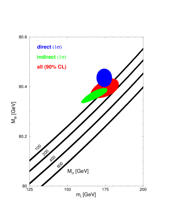
Figure 1: Direct and indirect determinations of $M_{W}$ and $m_{t}$. The bands are the SM predictions for various values of $M_{H}$, their widths indicating the uncertainties from other inputs.

2 $M_{H}$

From the precision data I obtain the result,

$$M_{H}=86^{+48}_{-32}\mbox{~{}GeV},$$ (1)

i.e., a 58% determination. The central value is 27 GeV or $0.6\sigma$ below the direct lower limit from LEP 2, $M_{H}>113.2$ GeV (95% CL) [6] The 90% central confidence interval is

$$38\hbox{ GeV}<M_{H}<173\hbox{ GeV}.$$ (2)

However, for a proper upper bound one should also take into account the direct search results at LEP 2, i.e. the exclusion of a Higgs boson with mass below 110 GeV or so, and the observation of several candidate events consistent with $M_{H}$ around 115 GeV. Making use of Bayes’ theorem [7],

$$p(M_{H}|{\rm data})=\frac{p({\rm data}|M_{H})p(M_{H})}{p({\rm data})},$$ (3)

one can compute the entire probability distribution function of $M_{H}$ conditional on the data and the validity of the SM. While the numerator, $p({\rm data})$, is easily obtained by properly normalizing the posterior probability density on the left-hand side, the prior probability, $p(M_{H})$, demands some extra thought:

Depending on the case at hand, the prior can (i) contain additional information not included in the likelihood model, (ii) contain likelihood information obtained from previous measurements, or (iii) be chosen non-informative. As for the present case, I choose the informative prior, $p(M_{H})=Q_{\rm LEP~{}2}~{}p^{\rm non-inf}(M_{H})$, where the non-informative part of the prior is,

$$p^{\rm non-inf}(M_{H})=M_{H}^{-1}.$$ (4)

The quantity,

$$Q_{\rm LEP~{}2}=\frac{{\cal L}({\rm data|signal+background})}{{\cal L}({\rm data|background})},$$ (5)

is an $M_{H}$ dependent summary statistic of the Higgs searches at LEP 2. If the signal hypothesis gives a better (worse) description of the data than the background only hypothesis one finds a negative (positive) contribution to the total $\chi^{2}$. Note, that this is a consistent treatment also in the case of a large downward fluctuation of the background or even if no events are observed at all. See the talk by Giuseppe Degrassi for more details and a somewhat different perspective [8].

The choice (4) corresponds to a flat prior in the variable $\ln M_{H}$, and there are various ways to justify it. One rationale is that a flat distribution is most natural for a variable defined over all the real numbers. This is the case for $\ln M_{H}$ but not $M_{H}^{2}$. Also, it seems that a priori it is equally likely that $M_{H}$ lies, say, between 30 and 40 GeV, or between 300 and 400 GeV. In any case, the sensitivity of the posterior to the (non-informative) prior diminishes rapidly with the inclusion of more data. Both, $p(M_{H})$ and $p^{\rm non-inf}(M_{H})$, are improper (not integrable) distributions, but the likelihood, $p({\rm data}|M_{H})$, constructed from the precision measurements assures a proper posterior.

Occasionally, the Bayesian method is criticized for the need of a prior, which would introduce unnecessary subjectivity into the analysis. Indeed, care and good judgement is needed, but the same is true for the likelihood model, which has to be specified in any statistical model. Moreover, it is appreciated among Bayesian practitioners, that the explicit presence of the prior can be advantageous: it manifests model assumptions and allows for sensitivity checks. From the theorem (3) it is also clear that any other method must correspond, mathematically, to specific choices for the prior. Thus, Bayesian methods are more general and differ rather in attitude: by their strong emphasis on the entire posterior distribution and by their first principles setup.

Figure 2: Probability distribution function [9] for the Higgs boson mass. The probability is shown for bin sizes of 1 GeV. Included are all available direct and indirect data. The shaded and unshaded regions each mark 50% probability.

Including $Q_{\rm LEP~{}2}$ in this way, one obtains the 95% CL upper limit $M_{H}\leq 201$ GeV, i.e. notwithstanding the observed excess events, the information provided by the Higgs searches at LEP 2 increases the upper limit by 28 GeV.

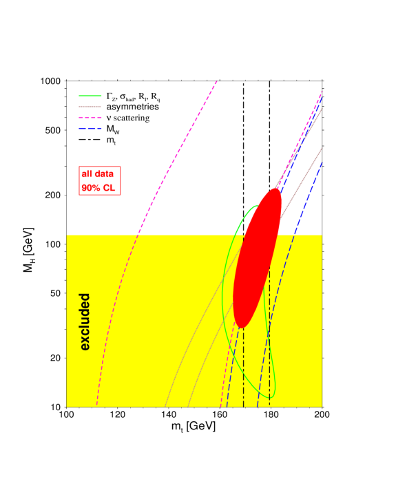
Figure 3: Current $1\sigma$ constraints on $M_{H}$ and $m_{t}$ from various precision observables. Their combination results in the red (solid) ellipse which contains 90% probability. The direct limit from LEP 2 is also indicated.

Given extra parameters, $\xi^{i}$, the distribution function of $M_{H}$ is defined as the marginal distribution, $p(M_{H}|{\rm data})=\int p(M_{H},\xi^{i}|{\rm data})\prod_{i}p(\xi^{i})d\xi^{i}$. If the likelihood factorizes, $p(M_{H},\xi^{i})=p(M_{H})p(\xi^{i})$, the $\xi^{i}$ dependence can be ignored. If not, but $p(\xi^{i}|M_{H})$ is (approximately) multivariate normal, then

$$\chi^{2}(M_{H},\xi^{i})=\chi^{2}_{\rm min}(M_{H})+{1\over 2}\frac{\partial^{2}\chi^{2}(M_{H})}{\partial\xi_{i}\partial\xi_{j}}(\xi^{i}-\xi^{i}_{\rm min}(M_{H}))(\xi^{j}-\xi^{j}_{\rm min}(M_{H})).$$ (6)

The latter applies to our case, where $\xi^{i}=(m_{t},\alpha_{s},\alpha(M_{Z}))$. Integration yields,

$$p(M_{H}|{\rm data})\sim\sqrt{\det E}\,e^{-\chi^{2}_{\rm min}(M_{H})/2},$$ (7)

where the $\xi^{i}$ error matrix, $E=(\frac{\partial^{2}\chi^{2}(M_{H})}{\partial\xi_{i}\partial\xi_{j}})^{-1}$, introduces a correction factor with a mild $M_{H}$ dependence. It corresponds to a shift relative to the standard likelihood model given by

$$\Delta\chi^{2}(M_{H})\equiv\ln\frac{\det E(M_{H})}{\det E(M_{Z})}.$$ (8)

This effect tightens the $M_{H}$ upper limit by 1 GeV. I also include theory uncertainties from uncalculated higher orders. This increases the upper limit by 5 GeV and finally yields

$$M_{H}\leq 205\mbox{ GeV}\mbox{ (95\% CL)}.$$ (9)

The entire probability distribution is shown in Fig. 2. Taking the data at face value, there is (as expected) a significant peak around $M_{H}=115$ GeV, but more than half of the probability is for Higgs boson masses above the kinematic reach of LEP 2 (the median is at $M_{H}=119$ GeV). However, if one would double the integrated luminosity and assume that the results would be similar to the present ones, one would find most of the probability concentrated around the peak. A similar statement will apply to Run II of the Tevatron at a time when about 3 to 5 ${\rm fb}^{-1}$ of data have been collected.

The current status of Higgs mass constraints can also be summarized graphically in the $M_{H}$–$m_{t}$ plane. Fig 3 shows the contours arising from the $Z$ lineshape measurements; from $Z$ pole asymmetries; from neutrino-hadron and neutrino-electron scattering; and from $M_{W}$. The direct measurement of $m_{t}$ from the Tevatron, and the direct lower limit on $M_{H}$ from LEP 2 are also shown. Notice, that all groups of measurements are consistent with each other and the SM, provided $M_{H}$ is not much larger than its current lower limit.

3 $\alpha_{s}$

Another fundamental SM parameter is the strong coupling constant, $\alpha_{s}$. Remarkably, within the SM the cleanest determination of the QCD coupling comes from electroweak physics. Table 1 shows the constraints on $\alpha_{s}$ provided by various electroweak observables. A few comments:

• The quoted errors include the uncertainty from $M_{H}$ which is allowed as a free parameter.

• The results are virtually unchanged if $M_{H}$ is fixed to 115 GeV instead, corresponding to the most likely value according to Fig. 2.

• The results are insensitive to types of new physics which couple preferentially to vector boson self-energies (“oblique corrections”; see Section 4). $\alpha_{s}=0.1201\pm 0.0031$ allowing the oblique STU parameters introduced in Ref. [10].

• The extracted $\alpha_{s}$ is very sensitive to non-universal new physics (to the $Zb\bar{b}$-vertex, etc.).

• It is amusing that the electroweak fit provides a more precise value than the QCD average, $\alpha_{s}=0.1184\pm 0.0031$ [11]. Authors addressing the combination of intrinsic QCD determinations of $\alpha_{s}$ feel uncomfortable with standard statistical procedures to combine information from various sources. This is mainly because (i) most uncertainties are strongly dominated by theory errors which oftentimes are no more than “best guesses”; (ii) there may be unknown correlations and common sources of uncertainties hampering straightforward averaging procedures. As a reasonable but subjective countermeasure, one chooses a very conservative attitude and inflates the error bars in a more or less ad hoc manner.

• The global fit result in Table 1 cannot be obtained by averaging the individual values due to both, experimental and theoretical (mainly from common inputs) correlations. While these represent major complications, they can be addressed effectively and unambiguously in a global fit (unlike in the QCD world average discussed before).

$\Gamma_{Z}$	$\alpha_{s}=0.1182\pm 0.0054$
$\sigma_{\rm had}$	$\alpha_{s}=0.1074\pm 0.0073$
$R_{e}$	$\alpha_{s}=0.1299\pm 0.0083$
$R_{\mu}$	$\alpha_{s}=0.1267\pm 0.0054$
$R_{\tau}$	$\alpha_{s}=0.1160\pm 0.0072$
global fit	$\alpha_{s}=0.1195\pm 0.0028$

Table 1: $\alpha_{s}$ from electroweak physics. $\Gamma_{Z}$ is the total $Z$ width, $\sigma_{\rm had}$ is the hadronic cross section on the $Z$ peak, while the $R_{\ell}$ are the three ratios of hadronic to leptonic $Z$ decay widths.

4 $S$ and $T$

The so called oblique parameters, such as the $S$, $T$, and $U$ parameters of Peskin and Takeuchi [10], are defined for types of new physics which (i) have no or negligible direct couplings to the standard fermions, and (ii) which have an associated mass scale much larger than $M_{Z}$. One example are non-standard contributions to the $\rho$ parameter, which measures the difference in the radiative corrections to the $W$ propagator relative to the $Z$ propagator. In fact, the $\rho_{0}$ parameter is trivially related to the Peskin-Takeuchi parameter, $T$, through

$$\rho_{0}={1\over 1-\alpha T},$$ (10)

where by definition, $\rho_{0}=1$ in the SM. The $S$ parameter, measures essentially the difference of the contributions to the $Z$ propagator at $q^{2}=M_{Z}^{2}$ relative to $q^{2}=0$. For example, a degenerate chiral fermion doublet gives a positive definite contribution to $S$ given by,

$$S=\sum\limits_{i}{[t_{3L}(i)-t_{3R}(i)]^{2}\over 3\pi}=\frac{4\hat{s}\hat{c}}{\hat{\alpha}}\frac{\Pi^{\rm new}_{ZZ}(M_{Z}^{2})-\Pi^{\rm new}_{ZZ}(0)}{M_{Z}^{2}},$$ (11)

where $t_{3L,R}$ denote the third component of isospin for the left and right-handed helicities, respectively, and $\hat{s}\hat{c}/\hat{\alpha}$ is a combination of gauge couplings. A global fit with $S$ allowed gives,

$$S=+0.10^{+0.13}_{-0.23},$$ (12)

and simultaneously $M_{H}=42^{+166}_{\,\,\,-26}$ GeV. Notice, the much larger error on $M_{H}$ compared to the SM fit. This is because $S$ and $M_{H}$ are almost perfectly anticorrelated with a correlation of $-94\%$. Thus, in the presence of the $S$ parameter, the $M_{H}$ constraints are significantly weakened and we find the upper bound $M_{H}<397$ GeV at the 95% CL.

Figure 4: Current $1\sigma$ constraints on $S$ and $T$ from various precision observables.

If $M_{H}$ is fixed at 115 GeV, we find $S=-0.033\pm 0.064$. We can use this result to find constraints on extra degenerate fermion doublets. For example, a sequential or mirror family of fermions contributes $\Delta S=+{2\over 3\pi}$. From the expression

$$\frac{e^{-\chi^{2}(N_{g}=3)/2}}{e^{-\chi^{2}(N_{g}=3)/2}+e^{-\chi^{2}(N_{g}=4)/2}},$$ (13)

we can therefore conclude that a degenerate 4th family is excluded at the 99.92% CL. Or we can turn things around and compute the number of extra families from the $S$ parameter, $N_{g}=2.84\pm 0.30$. This is complementary to $N_{\nu}=2.986\pm 0.008$ arrived at from neutrino counting at LEP 1, which now shows a deviation of $1.7\sigma$ from the SM prediction of $N_{\nu}=3$. In essence, this is a consequence of the measured $\sigma_{\rm had}$ which deviates by the same amount.

The results on the $S$ and $T$ parameters (with $U=0$) are summarized in Fig. 4, again broken down into various subsets of observables: the $Z$ lineshape measurements; $Z$ pole asymmetries; neutrino scattering; $M_{W}$; and $Q_{W}$. It is seen that the precision data is consistent with the SM prediction, $S=T=0$, in particular if $M_{H}$ is relatively light.

One also sees that the $S$ parameter is strongly correlated with $T$. Repeating the fit with $T$ allowed yields $N_{g}=3.02\pm 0.46$ and $T=0.06\pm 0.12$. Thus, the constraints are weaker for a non-degenerate 4th family.

References

- [1] W. J. Marciano and A. Sirlin, Phys. Rev. D 22, 2695 (1980). U. Amaldi et al., Phys. Rev. D 36, 1385 (1987). G. Degrassi, S. Fanchiotti and A. Sirlin, Nucl. Phys. B351, 49 (1991). G. Degrassi and A. Sirlin, Nucl. Phys. B352, 342 (1991). S. Fanchiotti, B. Kniehl and A. Sirlin, Phys. Rev. D 48, 307 (1993) [hep-ph/9212285]. P. Gambino and A. Sirlin, Phys. Rev. D 49, 1160 (1994) [hep-ph/9309326].
- [2] J. Erler, hep-ph/0005084. http://www.physics.upenn.edu/erler/electroweak/GAPP.html.
- [3] P. Langacker, these proceedings.
- [4] A. Derevianko, Phys. Rev. Lett. 85, 1618 (2000) [hep-ph/0005274].
- [5] J. Erler and P. Langacker, Phys. Rev. Lett. 84, 212 (2000) [hep-ph/9910315].
- [6] T. Junk, Combined LEP Higgs Searches, Talk presented at the LEP Fest 2000, CERN, October 2000.
- [7] T. Bayes, Philos. Trans. R. Soc. 53, 370 (1763), reprinted in Biometrika 45, 293 (1958).
- [8] G. Degrassi, these proceedings.
- [9] J. Erler, hep-ph/0010153.
- [10] M. E. Peskin and T. Takeuchi, Phys. Rev. Lett. 65, 964 (1990).
- [11] S. Bethke, J. Phys. G26, R27 (2000) [hep-ex/0004021].