UCB-PTH-01/04

LBNL-47413

HUTP-01/A006

UW/PT-01/01

Finite Radiative Electroweak Symmetry Breaking
from the Bulk

Nima Arkani-Hamed^a,b,c, Lawrence Hall^a,b, Yasunori Nomura^a,b,
David Smith^a,b and Neal Weiner^d

^a Department of Physics, University of California, Berkeley, CA 94720
^b Theoretical Physics Group, Lawrence Berkeley National Laboratory, Berkeley, CA 94720
^c Jefferson Physical Laboratory, Harvard University, Cambridge, MA 02138
^d Department of Physics, University of Washington, Seattle, WA 98195

1 Introduction

The physical origin of the mass scale of electroweak symmetry breaking (EWSB) is unknown. In technicolor theories, the mass scale of EWSB has a direct physical interpretation as the scale at which some new gauge force becomes strong. In supersymmetric theories, the scale of EWSB is related to the scale of supersymmetry breaking, although the connection is often indirect and model dependent [1, 2]. In this paper we introduce a mechanism which requires the EWSB scale to be directly connected to the length scale of a new compactified spatial dimension.

The physical mechanism for EWSB is also unknown. Precision electroweak data suggest that there is a perturbatively coupled Higgs boson [3], and it is this possibility that we explore. The large value of the top-quark mass implies that the Higgs boson has a Yukawa coupling to the top quark, $y_{t}$, which is close to unity. This leads to a one-loop quadratic divergence in the Higgs-boson mass-squared parameter

$$m_{H}^{2}=m_{H0}^{2}-{N_{c}\,y_{t}^{2}\over 4\pi^{2}}\Lambda^{2},$$ (1)

where the standard model is viewed as a low energy effective theory valid up to some cutoff $\Lambda$, and $m_{H0}^{2}$ is the tree-level mass parameter. Given the negative sign of this radiative correction, it is tempting to infer that it is this radiative correction which is triggering EWSB. However, this conclusion cannot be drawn — the quadratic divergence implies that the scale of the physics triggering EWSB is at $\Lambda$, where the low energy effective theory breaks down and is unreliable. In this sense, the standard model does not provide a theory of EWSB. For $\Lambda$ larger than a few TeV, the cancellation between the tree and radiative terms in Eq. (1) becomes problematic.

In supersymmetric theories the quadratic divergence of the Higgs mass parameter from the top-quark loop is cancelled by that from the top-squark loop. The residual divergence is logarithmic

$$m_{H}^{2}=m_{H}^{2}(\Lambda)-{N_{c}\,y_{t}^{2}\over 4\pi^{2}}\,m_{\tilde{t}}^{2}\ln{\Lambda^{2}\over m_{\tilde{t}}^{2}},$$ (2)

with the mass scale of the radiative correction determined by the top-squark mass, $m_{\tilde{t}}$ [4]. Here $\Lambda$ is again understood to be the ultraviolet cutoff of the supersymmetric theory containing soft supersymmetry-breaking parameters. Such theories have gained much attention over the last two decades because, for large values of the logarithm, the radiative triggering of EWSB is reliably computed in the low energy theory — one has a theory of EWSB.

What is the energy scale of the physics that triggers EWSB in supersymmetric theories? The logarithmic divergence implies that the Higgs mass parameter can be viewed as running with scale, so that the physics of EWSB is the evolution of this parameter with energy. The energy region where most of this evolution occurs is model dependent — it can be anywhere between the top-squark mass, which sets the mass scale of the electroweak vacuum expectation value, and the ultraviolet cutoff, $\Lambda$.

In supersymmetric theories the quartic Higgs coupling is predicted, leading to a well known upper bound on the Higgs mass of about 135 GeV [5]. Also, in the absence of fine-tuning, the physical Higgs mass-squared is given by the size of the radiative correction, and is therefore expected to be $(m_{\tilde{t}}^{2}/10)\ln(\Lambda^{2}/m_{\tilde{t}}^{2})$. For large values of the logarithm, as in gravity mediated theories, the top squark is not expected to be much heavier than the Higgs boson, so that typically $m_{\tilde{t}}\mathop{}_{\textstyle\sim}^{\textstyle<}200$ GeV, conflicting with data. For small values of the logarithm, as in certain gauge mediated theories, it is most natural for the top squark to be a factor 3 heavier than the Higgs boson. But in these theories the charged slepton and winos are significantly lighter than the top squark, and the direct searches at LEP imply that the top-squark mass is well above three times the Higgs mass. Thus, in the most-studied supersymmetric theories, we already know that EWSB does not occur in the most natural region of parameter space [6]. The amount of parameter tuning is modest, and this analysis fuels an expectation that superpartners may well be discovered soon.

In this paper we introduce a new mechanism for radiative EWSB in supersymmetric theories. The divergence in the Higgs mass is cut off by the scale of a new compact dimension of TeV size. The radiative Higgs mass is calculable and finite, and dominated by physics at the TeV scale. Our mechanism relies on a departure from previous models with TeV-sized extra dimensions [7, 8, 9, 10], which have brane-localized matter fields. Two crucial ingredients are required in our framework:

• The virtual top quarks and top squarks in the radiative diagrams for the Higgs-boson mass propagate in the new compact dimension.

• The top-quark Yukawa coupling and the breaking of supersymmetry are not located at the same point in the bulk.

This implies that, in the radiative Higgs mass calculation, the virtual propagators of the top-quark multiplet must sample the bulk far from the Yukawa interaction to avoid an exact supersymmetric cancellation. If this distance scale is $D$, then the contributions from large virtual 4-momentum, $k$, to the Higgs mass are exponentially suppressed by $e^{-kD}$. The resulting radiative contribution to the Higgs mass-squared parameter is found to be finite: $m_{H}^{2}=m_{H0}^{2}-C(N_{c}y_{t}^{2}/\pi^{2})(1/D)^{2}$, where $C$ is a model dependent parameter of order unity. Comparing with the standard model result of Eq. (1), we see that the quadratic divergence is regulated by the spatial separation in the bulk. Contrary to previous models, the quadratic divergence of the Higgs boson mass is directly cut off at the distance scale $D$; in no energy region is the Higgs boson mass logarithmically sensitive to the cutoff of the effective theory.

What is the scale $D$ which governs the separation of supersymmetry breaking and flavor breaking? In this paper we take the bulk to preserve supersymmetry, forcing the top-quark Yukawa coupling to be localized on some “Yukawa brane”. One possibility is that $D$ is simply the distance across the bulk from the Yukawa brane to the closest brane on which there is supersymmetry breaking. However, we have an alternative picture in mind. The relevant scale is the distance scale on which the top-quark multiplet feels supersymmetry breaking. We assume that the top multiplet feels supersymmetry breaking via the form of its mode expansion in the bulk — ie supersymmetry breaking forces the Kaluza-Klein (KK) expansion of the top quarks to differ from that of the top squarks. Since the dimensionful parameter of the KK mode expansion is the radius of the bulk, $R$, we expect $D\approx R$. In this paper we study theories with a one dimensional bulk, taken to be the $S^{1}/Z_{2}$ orbifold, so that the distance is the length of the orbifold, $D=\pi R$, giving

$$m_{H}^{2}=-C{N_{c}\,y_{t}^{2}\over\pi^{4}}\left({1\over R}\right)^{2}.$$ (3)

We have set $m_{H0}^{2}=0$ — our EWSB mechanism only works if the tree-level Higgs soft mass is small, and, in the theories considered in this paper, it vanishes.

Electroweak symmetry is broken radiatively by the large top-quark Yukawa interaction, but locality exponentially cuts off supersymmetry breaking at short distances. The top multiplet propagators are supersymmetric at high energies, apart from $e^{-k\pi R}$ corrections, so that EWSB is necessarily broken by physics at the compactification scale. From Eq. (3) we see that there is a very close relationship between the Higgs mass and the compactification scale: the physical Higgs mass is about $0.2(1/R)$. Our EWSB mechanism has no naturalness problem; the Higgs boson is lighter than the KK resonances by a loop factor.

What is the general structure of the theory just above the weak scale? This is the crucial question for future collider physics. With conventional radiative EWSB there are superpartners, since we have an energy region described by a 4d supersymmetric theory. However, with our mechanism there is no energy interval where physics is described by a 4d supersymmetric theory. Just above the weak scale we have a 5d theory, which has two supersymmetries from the 4d viewpoint. As well as the usual superpartners, there are the “$N=2$” partners and KK resonances, all having mass splittings determined by $1/R$. The spectrum of this large number of states is model dependent, but, in the models described below, is given in terms of just a few free parameters. The presence of these extra states is a necessary consequence of our new EWSB scheme, with the Higgs mass divergence regulated by 5d supersymmetry, broken at the compactification scale $1/R$. The physics of EWSB is the physics of the spectrum of these states near $1/R$. Unlike the 4d supersymmetric case, physics at scales much larger than the weak scale is irrelevant.

In section 2 we perform a calculation of the Higgs mass-squared using KK towers of the top quarks and top squarks which are shifted relative to each other to reflect supersymmetry breaking. We show in detail how the Bose and Fermi loop contributions, when summed over the entire KK tower, lead to the finite Higgs mass result of Eq. (3), with a parameter $C$ close to unity. This provides a general illustration of our EWSB mechanism, but leaves two issues open: what is the underlying mechanism of supersymmetry breaking, and what provides the restoring potential for the Higgs field?

We study two possibilities for supersymmetry breaking — local and non-local in the bulk. In sections 3 and 4 we study two explicit models, illustrating local and non-local supersymmetry breaking respectively. In section 3 supersymmetry breaking is localized on a three brane, and is coupled directly to the zero-mode top squark, resulting in a non-uniform profile for its wavefunction in the bulk. In section 4 supersymmetry is broken by the Scherk-Schwarz mechanism [12] using $R$ parity: under a translation about the circle by $2\pi R$ the top-squark wavefunction is required to change sign, while the top-quark wavefunction is invariant. These models illustrate the general properties of supersymmetry breaking that we require: at short distances, whether near the Yukawa brane or at a typical point in the bulk, all interactions are supersymmetric. The supersymmetric cancellation in the Higgs mass calculation is prevented because the top-multiplet KK modes feel supersymmetry breaking in their wavefunctions on distance scales of order $R$. In sections 3 and 4 we also compute the Higgs mass without performing a KK decomposition of the top multiplet, by studying the propagators of the top multiplet in position space in the bulk. This calculation demonstrates the insensitivity of our results to ultraviolet physics — one only needs a reliable effective theory at the energy scale $1/R$, since contributions from 4-momenta above this are exponentially damped. It also demonstrates the 5d supersymmetric cancellation more clearly than the KK mode calculation.

In section 5 we discuss Higgs sectors on the Yukawa brane which successfully give masses to the Higgsinos and provide a restoring potential for the Higgs field. The phenomenology of our theories is briefly studied in section 6, with emphasis on the different nature of the lightest superparticle (LSP) in the various models. Our conclusions are drawn in section 7.

The model of section 3 also illustrates a new dynamical solution to the supersymmetric flavor problem. Even though squarks of the three generations have different couplings to the supersymmetry-breaking brane, the resulting squark wavefunctions are nearly identical, giving near degeneracy, as long as these couplings are all large.

2 Radiative Correction to the Higgs-Boson Mass

2.1 Framework

In this paper, we work in a framework of 5d supersymmetric models with the fifth dimension compactified on an $S^{1}/Z_{2}$ orbifold. The minimal supersymmetric multiplets in 5d are hypermultiplets and vector supermultiplets. The vector supermultiplet contains two Weyl fermions $\lambda_{1}$ and $\lambda_{2}$, a five-vector gauge field $A_{M}$, and a real scalar $\sigma$, all in the adjoint representation. The hypermultiplet contains two complex scalars $\phi$ and $\phi^{c}$ and two Weyl fermions $\psi$ and $\psi^{c}$. Under the 4d $N=1$ supersymmetry, the vector supermultiplet fields form a vector superfield $V(\lambda_{1},\;A_{\mu})$ and an adjoint chiral superfield $\Sigma({1\over\sqrt{2}}(\sigma+iA_{5}),\;\lambda_{2})$, while the hypermultiplet fields form two chiral superfields, $\Phi(\phi,\;\psi)$ and $\Phi^{c}(\phi^{c},\;\psi^{c})$, with opposite quantum numbers.

When we compactified the extra dimension on $S^{1}/Z_{2}$, we have two different types of fields; the bulk fields and the brane fields. Let us label the coordinate $y$ of the extra dimension such that the orbifold fixed points are at $y=0$ and $y=\pi R$, where the $Z_{2}$ identifies points under the reflection $y\leftrightarrow-y$. The bulk fields propagate in all five dimensions, and are classified according to whether they have an even or odd transformation under the $Z_{2}$ reflection. Since the form of the Lagrangian requires that $\Phi$ and $\Phi^{c}$, and $V$ and $\Sigma$, have opposite transformation property, we take

$$\Phi(x,-y)=\Phi(x,y),\qquad\Phi^{c}(x,-y)=-\Phi^{c}(x,y),$$ (4)

$$V(x,-y)=V(x,y),\qquad\Sigma(x,-y)=-\Sigma(x,y).$$ (5)

Note that the odd fields such as $\Phi^{c}$ and $\Sigma$ do not have zero modes after the KK decomposition. Therefore, the orbifold compactification breaks the original 5d supersymmetry to 4d $N=1$ supersymmetry in the zero-mode sector. On the other hand, the brane fields are localized on the orbifold fixed point, and can propagate only on the four dimensional hypersurface. Thus, they form 4d $N=1$ supersymmetry multiplets and do not have any KK towers after the KK decomposition.

Throughout the paper, we take all three generations of standard-model quarks and leptons, contained in hypermultiplets, and all standard-model gauge fields, contained in vector supermultiplets, to propagate in the extra dimension. That is, chiral superfields $Q$, $U$, $D$, $L$, and $E$ propagate in the bulk along with their conjugate superfields $Q^{c}$, $U^{c}$, $D^{c}$, $L^{c}$, and $E^{c}$, and each vector superfield $V$ is accompanied by the corresponding chiral adjoint $\Sigma$. The quark and lepton multiplets interact with the Higgs fields through the 4d $N=1$ supersymmetric Yukawa interactions located on the orbifold fixed point at $y=0$ (the Yukawa brane). The two Higgs doublets $H_{u}$ and $H_{d}$ are required to give both up-type and down-type quark masses. They can be either bulk or brane fields. If the Higgs fields are the bulk fields, they are accompanied by the conjugate fields, $H_{u}^{c}$ and $H_{d}^{c}$.

Once supersymmetry is broken, the masses of the squark tower are shifted relative to those of the quark tower, and this effect is transmitted to the Higgs boson through radiative corrections. Here we consider a class of models where the Higgs soft masses are zero at the tree level even after supersymmetry breaking. Two explicit examples for such theories are given in section 3 and section 4. Then, the Higgs scalars receive soft masses only radiatively through the loops of the bulk quark multiplets. In the next subsection, we explicitly calculate the one-loop radiative correction to the up-type Higgs-boson mass coming from the loops of the KK towers of the top-quark hypermultiplets through the top-Yukawa coupling on the Yukawa brane. We find that the result is finite in contrast to the usual 4d supersymmetric models where it is logarithmically divergent. We also show that the correction is negative, so that it can indeed trigger EWSB. A complete discussion of the Higgs sector will be postponed until section 5.

2.2 Calculation of the Higgs mass-squared

In this subsection, we derive formulae for the radiatively generated Higgs-boson mass-squared, assuming that the Higgs boson is a brane field. However, the final formulae written in terms of the 4d top-Yukawa coupling are also correct in the case where the Higgs boson is a bulk field, and are applicable in a class of extra dimensional theories discussed in sections 3 and 4.

We calculate the Higgs-boson mass by making a KK decomposition of the original 5d theory. After the KK decomposition, the kinetic terms for the KK modes of the quark fields are written in terms of the canonically normalized fields as

$$S_{\rm kin} = \int d^{4}x\Biggl{[}\Biggr{\{}\sum_{k=0}^{\infty}\Bigl{(}\partial^{\mu}\phi_{Q,k}^{\dagger}\partial_{\mu}\phi_{Q,k}-m_{\phi_{Q},k}^{2}\phi_{Q,k}^{\dagger}\phi_{Q,k}\Bigr{)}+\sum_{k=1}^{\infty}\Bigl{(}\partial^{\mu}\phi^{c\,\dagger}_{Q,k}\partial_{\mu}\phi^{c}_{Q,k}-m_{\phi_{Q}^{c},k}^{2}\phi^{c\,\dagger}_{Q,k}\phi^{c}_{Q,k}\Bigr{)}$$ (6)

$$+\sum_{k=1}^{\infty}\Bigl{(}\psi_{Q,k}^{\dagger}\,i\bar{\sigma}^{\mu}\partial_{\mu}\psi_{Q,k}+\psi^{c\,\dagger}_{Q,k}\,i\bar{\sigma}^{\mu}\partial_{\mu}\psi^{c}_{Q,k}-m_{\psi_{Q},k}\psi^{c}_{Q,k}\psi_{Q,k}-m_{\psi_{Q},k}\psi_{Q,k}^{\dagger}\psi^{c\,\dagger}_{Q,k}\Bigr{)}$$

$$+\psi_{Q,0}^{\dagger}\,i\bar{\sigma}^{\mu}\partial_{\mu}\psi_{Q,0}\Biggr{\}}+\Bigl{\{}Q\rightarrow U\Bigr{\}}\Biggr{]},$$

where $\phi_{X}$ and $\psi_{X}$ ($\phi^{c}_{X}$ and $\psi^{c}_{X}$) represent the scalar and fermion components of the chiral superfield $X$ ($X^{c}$), respectively.

The interactions between the Higgs fields and the KK modes of the quark fields are located on the $y=0$ fixed point:

$$S_{\rm Yukawa}=\int\!\!d^{4}\!x\,dy\;\delta(y)\left[-\int\!\!d^{2}\!\theta\left({f_{t}\over M_{*}}Q_{3}U_{3}H_{u}+{f_{b}\over M_{*}}Q_{3}D_{3}H_{d}+\cdots\right)+{\rm h.c.}\right],$$ (7)

where the the chiral superfields $Q,U$ and $D$ are normalized in 5d so that they have mass dimension $3/2$, and $M_{*}$ is the cutoff of the theory. Expanding the above brane interactions in component fields and eliminating the auxiliary $F$ fields, the relevant interactions between canonically normalized 4d fields are found to be

$$S_{\rm int} = \int d^{4}x\Biggl{[}\sum_{k=1}^{\infty}\sum_{l=0}^{\infty}\Bigl{(}f_{t}\epsilon\,m_{\phi_{Q}^{c},k}\eta^{F_{Q}}_{k}\eta^{\phi_{U}}_{l}\phi^{c\,\dagger}_{Q,k}\phi_{U,l}\phi_{H}+f_{t}\epsilon\,m_{\phi_{U}^{c},k}\eta^{F_{U}}_{k}\eta^{\phi_{Q}}_{l}\phi^{c\,\dagger}_{U,k}\phi_{Q,l}\phi_{H}+{\rm h.c.}\Bigr{)}$$ (8)

$$-\sum_{k=0}^{\infty}\sum_{l=0}^{\infty}\sum_{m=0}^{\infty}\Bigl{(}f_{t}^{2}\epsilon^{2}\eta^{\phi_{Q}}_{k}\eta^{\phi_{Q}}_{l}(\eta^{F_{U}}_{m})^{2}\phi^{\dagger}_{Q,k}\phi_{Q,l}\phi^{\dagger}_{H}\phi_{H}+f_{t}^{2}\epsilon^{2}\eta^{\phi_{U}}_{k}\eta^{\phi_{U}}_{l}(\eta^{F_{Q}}_{m})^{2}\phi^{\dagger}_{U,k}\phi_{U,l}\phi^{\dagger}_{H}\phi_{H}\Bigr{)}$$

$$-\sum_{k=0}^{\infty}\sum_{l=0}^{\infty}\Bigl{(}f_{t}\epsilon\,\eta^{\psi_{Q}}_{k}\eta^{\psi_{U}}_{l}\psi_{Q,k}\psi_{U,l}\phi_{H}+{\rm h.c.}\Bigr{)}\Biggr{]},$$

where $\epsilon$ is defined by $\epsilon\equiv 1/(\pi RM_{*})$. Here, $\eta^{\phi_{X}}_{k}$, $\eta^{\psi_{X}}_{k}$ and $\eta^{F_{X}}_{k}$ are the values of the wavefunctions at $y=0$ for the $\phi_{X,k}$, $\psi_{X,k}$ and $F_{X,k}$ fields, respectively.

The Higgs-boson mass $m_{\phi_{H}}$ is generated at the one-loop level via loops of KK towers of the $Q$ and $U$ multiplets. There are three types of diagrams, as shown in Fig. 1, giving the three contributions

$$-i\,m_{\phi_{H}}^{2} = N_{c}f^{2}\epsilon^{2}\sum_{k=1}^{\infty}\sum_{l=0}^{\infty}(\eta^{F_{Q}}_{k})^{2}(\eta^{\phi_{U}}_{l})^{2}\int\frac{d^{4}p}{(2\pi)^{4}}\frac{m_{\phi_{Q}^{c},k}^{2}}{(p^{2}-m_{\phi_{Q}^{c},k}^{2})(p^{2}-m_{\phi_{U},l}^{2})}+(Q\leftrightarrow U)$$ (9)

$$-2N_{c}f^{2}\epsilon^{2}\sum_{k=0}^{\infty}\sum_{l=0}^{\infty}(\eta^{\psi_{Q}}_{k})^{2}(\eta^{\psi_{U}}_{l})^{2}\int\frac{d^{4}p}{(2\pi)^{4}}\frac{p^{2}}{(p^{2}-m_{\psi_{Q},k}^{2})(p^{2}-m_{\psi_{U},l}^{2})}$$

$$+N_{c}f^{2}\epsilon^{2}\sum_{k=0}^{\infty}\sum_{l=0}^{\infty}(\eta^{\phi_{Q}}_{k})^{2}(\eta^{F_{U}}_{l})^{2}\int\frac{d^{4}p}{(2\pi)^{4}}\frac{1}{(p^{2}-m_{\phi_{Q},k}^{2})}+(Q\leftrightarrow U).$$

Figure 1: One-loop diagrams contributing to the Higgs-boson mass.

The exotic diagram, where the conjugate scalar fields $\phi^{c}_{Q,k}$ and $\phi^{c}_{U,k}$ circulate in the loop, is not present in the usual 4d supersymmetric models. This diagram is actually needed to ensure the cancellation of $m_{\phi_{H}}^{2}$ in the supersymmetric limit, $m_{\phi_{X},k}=m_{\phi_{X}^{c},k}=m_{\psi_{X},k}$ and $\eta^{\phi_{X}}_{k}=\eta^{\psi_{X}}_{k}=\eta^{F_{X}}_{k}$.

When supersymmetry is broken, the masses for the squark and quark towers shift relatively. We here assume that the KK mass spectrum and wavefunctions do not depend on the species $Q$ and $U$, for simplicity, and drop the subscript $X$ from all quantities hereafter. This assumption is indeed satisfied in a broad class of extra dimensional models, at least at the leading order in $1/(M_{*}R)$, including the two explicit models discussed later. Supersymmetry breaking effects are represented by the deviations of the KK masses and wavefunctions from their supersymmetric relations, such as $m_{\phi,k}=m_{\psi,k}$ and $\eta^{\phi}_{k}=\eta^{\psi}_{k}$. In general, the mass $m_{k}$ for the $k$-th KK excitation mode can be a rather complicated function of $k$; often it is even not equally spaced in $k$. However, here we focus on some simple cases in which the masses for some of the KK towers are shifted by half a unit of $1/R$, and illustrate the basic idea that the Higgs-boson mass-squared receives a finite and negative contribution from the loops of the KK towers of the quark multiplets. A more intuitive understanding of this remarkable property from the 5d viewpoint will be given in due course, in the context of explicit models.

We consider the following spectrum for the KK towers:

$$m_{\psi,k}=k\frac{1}{R}\qquad(k=0,1,2,\cdots),$$ (10)

$$m_{\phi,k}=(k+r^{\phi})\frac{1}{R}\qquad(k=0,1,2,\cdots),$$ (11)

$$m_{\phi^{c},k}=(k+r^{F})\frac{1}{R}\qquad\left(\left\{\begin{array}[]{ll}k=1,2,3,\cdots&{\rm for}\quad r^{F}=0\\ k=0,1,2,\cdots&{\rm for}\quad r^{F}=\frac{1}{2}\\ \end{array}\right.\right),$$ (14)

where $r^{\phi}$ and $r^{F}$ take the value $0$ or $1/2$. The supersymmetric limit corresponds to $r^{\phi}=r^{F}=0$. Since the $r^{\phi}=0$ case means massless squarks at the tree level and is outside of the framework here, we concentrate on the two cases $(r^{\phi},r^{F})=(1/2,0)$ and $(1/2,1/2)$ below. These two cases corresponds to two explicit models discussed in sections 3 and 4. The wavefunctions $g_{k}(y)$ for the KK modes are normalized such that $\int_{0}^{\pi R}[g_{k}(y)]^{2}dy=\pi R$, giving

$$\eta^{\psi}_{k}=(\frac{1}{\sqrt{2}})^{\delta_{k,0}},$$ (15)

$$\eta^{\phi}_{k}=1,$$ (16)

$$\eta^{F}_{k}=\left\{\begin{array}[]{ll}(\frac{1}{\sqrt{2}})^{\delta_{k,0}}&{\rm for}\quad r^{F}=0,\\ 1&{\rm for}\quad r^{F}=\frac{1}{2},\\ \end{array}\right.$$ (19)

where $k=0,1,2,\cdots$. Plugging Eqs. (10 – 19) into a general expression Eq. (9), we obtain the radiative correction to the Higgs-boson mass.

Performing a Wick rotation to Euclidean momentum space $p_{E}$, and changing to the variable $x=p_{E}R$, gives

$$-i\,m_{\phi_{H}}^{2} = \frac{iN_{c}f_{t}^{2}\epsilon^{2}}{R^{2}}\int\frac{d^{4}x}{(2\pi)^{4}}x^{2}$$ (20)

$$\times\sum_{k,l=0}^{\infty}\Biggl{[}\frac{(\eta^{\psi}_{k})^{2}(\eta^{\psi}_{l})^{2}}{(x^{2}+k^{2})(x^{2}+l^{2})}-\frac{(\eta^{\phi}_{k})^{2}(\eta^{F}_{l})^{2}}{(x^{2}+(k+r^{\phi})^{2})(x^{2}+(l+r^{F})^{2})}\Biggr{]}.$$

In this expression, we first sum over the infinite tower of KK states and then perform the momentum integral to obtain a sensible result. Given that higher dimensional theories are non-renormalizable and must be cut off at some scale, one might worry that summing up infinite KK states is not the correct procedure. However, the point is that any cutoff must preserve the correct symmetries of the theory; 5d Lorentz symmetry and supersymmetry. This is precisely what is done by summing up infinite towers of the KK states, and is difficult to attain in any other way. In that sense, we can view this summation procedure as a kind of regularization, “KK regularization”. Indeed, after the summation, the resulting momentum integral turns out to be strongly dominated by the $1/R$ scale and the contribution from near the cutoff scale is extremely small. This is also consistent with the 5d picture that the Higgs boson requires some non-local information over the $1/R$ scale to feel supersymmetry breaking, which we will explicitly see in later sections.

Now, let us evaluate the Higgs-boson mass using Eq. (20). It is easy to check that the expression vanishes in the supersymmetric limit $r^{\phi}=r^{F}=0$. In the case of $(r^{\phi},r^{F})=(1/2,0)$, the Higgs-boson mass is given by

$$m_{\phi_{H}}^{2} = -\frac{N_{c}f_{t}^{2}\epsilon^{2}}{16R^{2}}\int_{0}^{\infty}dx\frac{x^{3}}{\sinh^{2}[\pi x]}$$ (21)

$$= -\frac{3\,\zeta(3)}{32\pi^{4}}\frac{N_{c}f_{t}^{2}\epsilon^{2}}{R^{2}},$$ (22)

where $\zeta(x)$ is the Riemann’s zeta function. We find that the radiative correction $m_{\phi_{H}}^{2}$ is negative and EWSB is indeed triggered by the loops of the KK towers. Furthermore, the result is finite and ultraviolet insensitive; the momentum integral is exponentially cut off at $p_{E}\sim(\pi R)^{-1}$ as was promised earlier. This extreme softness seems to come from a miraculous cancellation between fermionic and bosonic KK modes from the 4d point of view. There is a beautiful understanding of this result from the 5d viewpoint, which will be discussed in the context of an explicit model in section 3, and more generally in the conclusion.

In the $(r^{\phi},r^{F})=(1/2,1/2)$ case, the Higgs mass-squared is

$$m_{\phi_{H}}^{2} = -\frac{N_{c}f_{t}^{2}\epsilon^{2}}{16R^{2}}\int_{0}^{\infty}dx\,x^{3}\left\{\coth^{2}[\pi x]-\tanh^{2}[\pi x]\right\}$$ (23)

$$= -\frac{21\,\zeta(3)}{128\pi^{4}}\frac{N_{c}f_{t}^{2}\epsilon^{2}}{R^{2}}.$$ (24)

As in the case of $(r^{\phi},r^{F})=(1/2,0)$, the radiative correction is negative and the momentum integral is exponentially cut off at $p_{E}\sim(\pi R)^{-1}$. This case occurs in the model given in section 4, where we also discuss a 5d interpretation of the result.

Finally, we can rewrite the expressions in Eqs. (22, 24) in terms of the 4d top-Yukawa coupling $y_{t}=f_{t}\epsilon/2$. They are given by

$$m_{\phi_{H}}^{2} = -\frac{3\,\zeta(3)}{8\pi^{4}}\frac{N_{c}\,y_{t}^{2}}{R^{2}}$$ (25)

$$\simeq -(1.39\times 10^{-2})\frac{y_{t}^{2}}{R^{2}},$$ (26)

for $(r^{\phi},r^{F})=(1/2,0)$ and

$$m_{\phi_{H}}^{2} = -\frac{21\,\zeta(3)}{32\pi^{4}}\frac{N_{c}\,y_{t}^{2}}{R^{2}}$$ (27)

$$\simeq -(2.43\times 10^{-2})\frac{y_{t}^{2}}{R^{2}},$$ (28)

for $(r^{\phi},r^{F})=(1/2,1/2)$. Here, we have used $N_{c}=3$ and $\zeta(3)\simeq 1.202$. Note that although the above results in Eqs. (25 – 28) are derived by assuming that the Higgs boson is a brane field, they are also valid in the case of the bulk Higgs field. This can be easily verified by carefully tracing the volume-suppression and wavefunction-normalization factors coming from the zero-mode Higgs boson.

The resulting values of $m_{\phi_{H}}^{2}$ are one-loop suppressed compared with $(1/R)^{2}$. This means that the superparticle masses can be naturally larger than the weak scale in contrast to the usual 4d supersymmetric models. If we consider $m_{\phi_{H}}\simeq 300~{}{\rm GeV}$, for instance, the compactification scale $R^{-1}$ can be as high as $R^{-1}\simeq(2\sim 3)~{}{\rm TeV}$, corresponding to the squark mass $(2R)^{-1}\simeq(1.0\sim 1.5)~{}{\rm TeV}$. This hierarchy between the squark and the Higgs-boson masses is a consequence of the fact that the Higgs soft mass is zero at the tree level.

3 Model with Localized Supersymmetry Breaking

In this and the next sections, we discuss two explicit models which realize the form of supersymmetry breaking discussed in the previous section. The two models have quite different mechanisms of realizing the desired properties: vanishing Higgs soft masses at the tree level and finiteness of the radiative correction to the Higgs-boson mass. We also give a useful physical picture to understand those properties in each model.

3.1 Setup

The first model we consider has the following structure. Let us consider two branes located at two orbifold fixed points, $y=0$ and $\pi R$. The two Higgs-doublet chiral superfields $H_{u}$ and $H_{d}$ are localized on the $y=0$ brane and the supersymmetry breaking occurs on the other brane at $y=\pi R$. A distinctive feature of the present model is that supersymmetry is strongly broken at the $y=\pi R$ fixed point by $\langle Z\rangle\sim M_{*}^{2}\theta^{2}$, where $Z$ is a chiral superfield localized at the fixed point and $M_{*}$ is the cutoff of the theory. This is easily realized by considering the brane superpotential

$$S_{Z}=\int\!\!d^{4}\!x\,dy\;\delta(y-\pi R)\left[\int\!\!d^{2}\!\theta M_{*}^{2}Z+{\rm h.c.}\right].$$ (29)

With this strong supersymmetry breaking, the bulk fields such as quark, lepton and gauge multiplets feel the supersymmetry breaking effect through the interactions with the $Z$ field.

The bulk fields and the brane fields confined on the orbifold fixed points can have localized interactions that respect the 4d $N=1$ supersymmetry. Thus, the bulk fields feel the supersymmetry breaking through the following interactions:

$$S_{\pi R} = \int\!\!d^{4}\!x\,dy\;\delta(y-\pi R)\left[-\int\!\!d^{4}\!\theta\left({c_{Q}\over M_{*}^{3}}Q^{\dagger}QZ^{\dagger}Z+{c_{U}\over M_{*}^{3}}U^{\dagger}UZ^{\dagger}Z+\cdots\right)\right.$$ (30)

$$\qquad\qquad\qquad\qquad+\left.\left(\int\!\!d^{2}\!\theta{1\over 16g_{5}^{2}}{c_{W}\over M_{*}^{2}}Z\,{\rm Tr}W^{\alpha}W_{\alpha}+{\rm h.c.}\right)\right].$$

Here the $c$’s are dimensionless, and $g_{5}$, the 5d gauge coupling, has mass dimension $-1/2$. We assume that the coupling constants $c$ are all positive. The wavefunctions of the fields that feel the supersymmetry breaking (the squarks, sleptons, and gauginos) will be repelled from the $y=\pi R$ fixed point, making their zero modes massive. This effect will be examined in detail in subsection 3.2.

The wavefunctions for fields odd under the $Z_{2}$ orbifold are forced to vanish at the fixed points, so that interactions like

$$\int\!\!d^{4}\!x\,dy\;\delta(y-\pi R)\int\!\!d^{4}\!\theta{1\over M_{*}^{3}}{Q^{c}}^{\dagger}Q^{c}Z^{\dagger}Z,$$ (31)

do not arise. Derivative interactions such as

$$\int\!\!d^{4}\!x\,dy\;\delta(y-\pi R)\int\!\!d^{4}\!\theta{1\over M_{*}^{5}}\partial_{y}{Q^{c}}^{\dagger}\partial_{y}Q^{c}Z^{\dagger}Z,$$ (32)

can exist, but will be suppressed by factors of $1/(RM_{*})$ for the lowest KK modes. From an effective field theory standpoint, it is completely consistent to couple only $\Phi$ and $V$ superfields to the orbifold fixed points and not $\Phi^{c}$ and $\Sigma$. It is nevertheless interesting that even if one includes couplings of the odd fields, they are naturally suppressed. In what follows we will for simplicity ignore the possible effects of supersymmetry breaking on the wavefunctions of $\Phi^{c}$ and $\Sigma$ fields. These effects, if present, would be smaller than those for the even field wavefunctions at lower KK modes, so the qualitative results we obtain should apply regardless.

Another important feature of the present model is that the Higgs chiral multiplets do not acquire a tree-level supersymmetry-breaking mass, since they are localized on the brane at $y=0$ and do not have any direct interactions with the $Z$ field. Therefore, they feel the supersymmetry breaking only radiatively through their couplings to the even bulk fields given in Eq. (7). Our model depends crucially on the Higgs soft mass being zero at the tree level, so that $m_{H_{u}}^{2}$ is driven negative by the large top-Yukawa coupling. In subsection 3.2 we will obtain the tree-level spectrum for the KK modes of the bulk fields, which will enable us to compute this radiative effect using the formulae of section 2. A complete discussion of the Higgs sector of our theory will be given in section 5.

3.2 Particle spectrum and radiatively induced $m_{H_{u}}^{2}$

Neither $\psi$ nor $\psi^{c}$ couples to the supersymmetry breaking, so they have the expansions

$$\psi(x,y)=\sum_{n=0}^{\infty}\frac{1}{\sqrt{2}^{\delta_{n,0}}}{\cos[ny/R]\over\sqrt{\pi R}}\psi_{n}(x),\qquad\psi^{c}(x,y)=\sum_{n=1}^{\infty}{\sin[ny/R]\over\sqrt{\pi R}}\psi^{c}_{n}(x).$$ (33)

The expansion of $A_{\mu}$ is completely analogous to that of $\psi$, and the expansions of the $Z_{2}$-odd scalars $\phi^{c}$ and $\sigma$ are analogous to that of $\psi^{c}$. Defining $M_{c}=1/R$, the masses of the KK modes are

$$m_{\psi,n}=m_{A^{\mu},n}=nM_{c}\qquad(n=0,1,2,\cdots),$$ (34)

and

$$m_{\psi^{c},n}=m_{\phi^{c},n}=m_{\sigma,n}=nM_{c}\qquad(n=1,2,\cdots).$$ (35)

For $n>0$, $\psi_{n}$ and $\psi_{n}^{c}$ marry to form a Dirac particle of mass $nM_{c}$. Note also that the non-zero modes of $A_{\mu}$ acquire mass by eating the corresponding modes of the odd scalar $A_{5}$.

The situation is more complicated for $\phi$ scalars because of their coupling to $F_{Z}$. Their classical equation of motion is

$$\partial_{\mu}^{2}\phi-\partial_{y}^{2}\phi+\delta(y-\pi R){c_{X}{F_{Z}}^{2}\over M_{*}^{3}}\phi=0,$$ (36)

where $X=Q,U,\cdots$. Remembering that $\phi$ is even under the $Z_{2}$, the solution (for $0<y<\pi R$) is

$$\phi(x,y)=\sum_{n=0}^{\infty}C_{n}\cos[m_{\phi,n}y]\phi_{n}(x),$$ (37)

where the $C_{n}$ are constants chosen to canonically normalize $\phi_{n}$ kinetic terms, and the 4d masses $m_{\phi,n}$ are the solutions to the equation

$$\tan[m_{\phi,n}\pi R]={c_{X}\over 2}{{F_{Z}}^{2}\over M_{*}^{4}}{M_{*}\over m_{\phi,n}}.$$ (38)

Taking $c_{X}\sim 1$ and $\sqrt{F_{Z}}\sim M_{*}$, one obtains

$$m_{\phi,n}\simeq\left(n+\frac{1}{2}\right)M_{c}\qquad(n=0,1,2,\cdots),$$ (39)

at the leading order in $M_{c}/M_{*}$. We see that at this order the supersymmetry breaking acts as an impenetrable wall that drives the wavefunction of $\phi_{n}$ to zero at $y=\pi R$, making the masses insensitive to the precise values of $c_{X}$ and $F_{Z}$. At the next order in $M_{c}/M_{*}$, one finds

$$m_{\phi,n}\simeq\left(n+\frac{1}{2}\right)M_{c}\left(1-{2\over c_{X}\pi}{M_{*}^{4}\over{F_{Z}}^{2}}{M_{c}\over M_{*}}\right),$$ (40)

giving a small but finite $\phi$ wavefunction at the supersymmetry-breaking brane.

The Weyl fermions $\lambda_{1}$ and $\lambda_{2}$ are coupled through their kinetic term, while only the even field $\lambda_{1}$ feels the supersymmetry breaking directly. The classical equations of motion are

$$-i{\overline{\sigma}}^{\mu}\partial_{\mu}\lambda_{2}+\partial_{y}{\overline{\lambda}}_{1}=0,$$ (41)

$$-i{\overline{\sigma}}^{\mu}\partial_{\mu}\lambda_{1}-\partial_{y}{\overline{\lambda}}_{2}-\delta(y-\pi R){c_{W}F_{Z}\over 2M_{*}^{2}}{\overline{\lambda}_{1}}=0.$$ (42)

Looking for solutions of the form

$$\lambda_{j}(x,y)=\eta_{j}(x)g_{j}(y)\qquad(j=1,2),$$ (43)

we find the boundary condition at the $y=\pi R$ fixed point

$$\eta_{2}(x)={c_{W}F_{Z}\over 4M_{*}^{2}}{g_{1}(\pi R)\over g_{2}(\pi R)}\,\eta_{1}(x).$$ (44)

Setting $i{\overline{\sigma}}^{\mu}\partial_{\mu}\eta_{1}=m_{\lambda}{\overline{\eta}_{1}}$ then leads to the solution

$$g_{1}\propto\cos[m_{\lambda}y],\qquad\qquad g_{2}\propto\sin[m_{\lambda}y],$$ (45)

with the KK-mode masses given by

$$\tan[m_{\lambda}\pi R]={c_{W}F_{Z}\over 4M_{*}^{2}}.$$ (46)

Note that Eq. (46) has solutions for both positive and negative $m_{\lambda}$ (the absolute value gives the physical mass). For instance, in the case of extremely weak supersymmetry breaking, with $\epsilon\equiv c_{W}F_{Z}/(4\pi M_{*}^{2})\ll 1$, the masses are given by $\epsilon M_{c}$, $(1\pm\epsilon)M_{c}$, $(2\pm\epsilon)M_{c}$, and so on. For the opposite case of very strong supersymmetry breaking, where $\delta\equiv 4M_{*}^{2}/(\pi c_{W}F_{Z})\ll 1$, the masses are $(1/2\pm\delta)M_{c}$, $(3/2\pm\delta)M_{c}$, etc.

Figure 2: Mass spectrum for the lowest KK modes of the bulk fields in our model, in the limit of very strong supersymmetry breaking, $\sqrt{F_{Z}}\gg M_{*}\gg M_{c}$. The fermion modes $\psi_{n}$ and $\psi^{c}_{n}$ form a Dirac state for $n>0$, while the modes of ${\lambda_{1}}$ and ${\lambda_{2}}$ combine to form nearly degenerate pairs of Majorana states.

The spectrum of states is summarized in Fig. 2 in the limit $\sqrt{F_{Z}}\gg M_{*}\gg M_{c}$. Lowering $\sqrt{F_{Z}}$ down to $M_{*}$ has only a small effect of order $M_{c}/M_{*}$ on the $\phi_{n}$ masses. In contrast, changes of order unity arise in the gaugino mass spectrum, unless $c_{W}\gg 1$. In particular, the near-degeneracy between pairs of their KK modes that exists in the strong supersymmetry-breaking limit is spoiled.

Knowing the KK expansions of $\psi$, $\phi$, and $\phi^{c}$ allows us to compute the one-loop induced mass-squared for the Higgs boson by applying the result of section 2. Using Eqs. (34, 35, 39), and taking $\eta_{k}^{\phi}=1$ and $\eta_{k}^{F}=\eta_{k}^{\psi}=(1/\sqrt{2})^{\delta_{k,0}}$ accordingly, we obtain the up-type Higgs-boson mass

$$m_{\phi_{H_{u}}}^{2}=-{3\,\zeta(3)\over 8\pi^{4}}N_{c}\,y_{t}^{2}M_{c}^{2},$$ (47)

from Eq. (25), since the KK mass spectrum in Fig. 2 corresponds to the $(r^{\phi},r^{F})=(1/2,0)$ case in section 2. We have also checked that the $O(M_{c}/M_{*})$ correction in the scalar mass in Eq. (40) gives only $O(M_{c}/M_{*})$ correction to the Higgs-boson mass and can be safely neglected.

3.3 5d interpretation

It is remarkable that the Higgs mass is not merely ultraviolet insensitive, but in fact ultraviolet finite. One might, however, be skeptical of this result. For instance, we have summed over all modes in the KK expansion, rather than merely those below the cutoff. If we were to introduce an explicit cutoff, a strong sensitivity to this cutoff would be present. Ordinarily a top-stop pair contributes to the Higgs mass an amount $\sim m^{2}_{\rm SUSY}/(16\pi^{2})$. Now that we have a tower, we would expect a multiplicity $N_{\rm KK}^{2}\simeq(M_{*}R)^{2}$ as well, which is what we find with an explicit cutoff. This result is incorrect, because when we sum the entire tower, we are in fact Fourier transforming to mixed position-momentum space [13]. In this formulation it is clear that the result must be finite, and the total summation of all modes is the proper thing to do.

Since the Yukawa brane is located at $y=0$ and the supersymmetry breaking is located at $y=\pi R$, for values of momenta $k_{4}>(\pi R)^{-1}$ the Higgs boson cannot simultaneously “see” both the Yukawa couplings and the supersymmetry breaking. Since the contribution to the Higgs mass relies on both of these, it must vanish exponentially at high momenta, just as we have seen in the previous calculation. This very intuitive result is masked by the KK formalism, despite its calculational utility. Here we will calculate in the mixed position-momentum space from the outset and these results will appear quite naturally.

To begin with, we must calculate the scalar propagator with the boundary mass term. We shall consider first the case of an infinite dimension before dealing with the compact case. We will work from the outset in Euclidean space. The equation for the Green’s function $G_{\phi}$ is

$$(-\partial_{4}^{2}-\partial_{y}^{2})G_{\phi}(x_{4},y)+m\delta(y-\pi R)G_{\phi}(x_{4},y)=\delta^{4}(x_{4})\delta(y),$$ (48)

where $m\equiv c_{X}F_{Z}^{2}/M_{*}^{3}$. Transforming to the mixed position-momentum space gives

$$(k_{4}^{2}-\partial_{y}^{2})\tilde{G}_{\phi}(k_{4},y)=-m\delta(y-\pi R)\tilde{G}_{\phi}(k_{4},\pi R)+\delta(y).$$ (49)

This is simply the equation for the one dimensional propagator of a field with mass $M=k_{4}$ and sources at $y=0$ and $y=\pi R$ with strengths one and $-m\tilde{G}_{\phi}(k_{4},\pi R)$, respectively. Knowing this, we can explicitly write the solution:

$$\tilde{G}_{\phi}(k_{4},y)=\frac{e^{-k_{4}|y|}}{2k_{4}}-m\tilde{G}_{\phi}(k_{4},\pi R)\frac{e^{-k_{4}|y-\pi R|}}{2k_{4}}.$$ (50)

We can solve for $\tilde{G}_{\phi}(k_{4},\pi R)$ and substitute back to get the complete result

$$\tilde{G}_{\phi}(k_{4},y)=\frac{e^{-k_{4}|y|}}{2k_{4}}-m\frac{e^{-k_{4}\pi R-k_{4}|y-\pi R|}}{(2k_{4})(2k_{4}+m)}.$$ (51)

As before we can take the $m\rightarrow\infty$ limit and get

$$\tilde{G}_{\phi}(k_{4},y)=\frac{e^{-k_{4}|y|}}{2k_{4}}-\frac{e^{-k_{4}2\pi R+k_{4}y}}{2k_{4}},$$ (52)

for $y<\pi R$ and

$$\tilde{G}_{\phi}(k_{4},y)=0,$$ (53)

for $y>\pi R$. Previously, we lacked an intuitive understanding of the $m\rightarrow\infty$ limit, where the result was insensitive to the value of $m$ so long as it was sufficiently high. Here we see that the supersymmetry-breaking brane reflects the $\phi$ field back and $m$ is a measure of the opacity. In the $m\rightarrow\infty$ limit, the wall becomes completely opaque, and the reflected signal is maximal.

      

Figure 3: Different contributions to the propagator from $y=0$ to $y=y^{\prime}$. In addition to the lowest order piece, there are both reflected contributions and winding contributions. In the $m\rightarrow\infty$ limit, the supersymmetry-breaking brane becomes opaque and the winding contributions vanish, although an infinite number of reflections contribute.

With this understanding, we can address the compact dimension case. The proper generalization of Eq. (48) is

$$(-\partial_{4}^{2}-\partial_{y}^{2})G_{\phi}(x_{4},y)+m\sum_{n}\delta(y-(2n+1)\pi R)G_{\phi}(x_{4},y)=\sum_{n}\delta^{4}(x_{4})\delta(y-2n\pi R),$$ (54)

where the summations now represent all possible windings, $n=-\infty,\cdots,\infty$. Then, using image charge techniques, one can calculate the propagator in complete analog with the infinite dimension case, finding

$$\tilde{G}_{\phi}(k_{4},y)=\frac{1}{2k_{4}}\frac{1}{\sinh[k_{4}\pi R]}\left\{\cosh[k_{4}(\pi R-y)]-\frac{m\cosh[k_{4}y]}{2k_{4}\sinh[k_{4}\pi R]+m\cosh[k_{4}\pi R]}\right\},$$ (55)

for $(y\in[0,\pi R])$. Again, we can take the opaque limit $m\rightarrow\infty$ and then the propagator becomes

$$\tilde{G}_{\phi}(k_{4},y)=\frac{1}{2k_{4}}\frac{1}{\sinh[k_{4}\pi R]}\left\{\cosh[k_{4}(\pi R-y)]-\frac{\cosh[k_{4}y]}{\cosh[k_{4}\pi R]}\right\}.$$ (56)

It is instructive to expand Eq. (56) in exponentials as

$$\tilde{G}_{\phi}(k_{4},y)=\frac{1}{2k_{4}}e^{-k_{4}y}-\frac{1}{2k_{4}}\left(e^{-k_{4}(2\pi R-y)}+e^{-k_{4}(2\pi R+y)}\right)\left(1-e^{-k_{4}2\pi R}+e^{-k_{4}4\pi R}-\cdots\right),$$ (57)

where the first term represents direct propagation and the second term represents contributions from reflections. In this expression, we can explicitly see that reflection from the supersymmetry-breaking brane just gives a minus sign: the reflection does not reduce the strength of the signal, implying that the supersymmetry-breaking brane is an ideal mirror in the limit $m\rightarrow\infty$. Note that we need not have resorted to solving Eq. (54) to get the propagator in Eq. (56). Since the wall is opaque, we could have found this result by summing all possible reflections from walls at $\pm\pi R$, picking up a minus sign at each reflection. The contributions to the propagator are represented in Fig. 3.

We also need the appropriate propagators for the $F$ components and fermions. Neither of the fields feel supersymmetry breaking directly, however, so it is relatively simple to calculate these.

For the $F$-component, we need only investigate the kinetic piece of the Lagrangian

$${\cal L}\supset\pmatrix{\phi^{c*}&F}\pmatrix{k_{4}^{2}&ik_{y}\cr ik_{y}&1}\pmatrix{\phi^{c}\cr F^{*}}.$$ (58)

We can invert this to yield

$$\pmatrix{k_{4}^{2}&ik_{y}\cr ik_{y}&1}^{-1}=\frac{1}{k_{4}^{2}+k_{y}^{2}}\pmatrix{1&-ik_{y}\cr-ik_{y}&k_{4}^{2}}.$$ (59)

Our $F$-$F$ propagator is just $k_{4}^{2}/(k_{4}^{2}+k_{y}^{2})$, which we trivially Fourier transform to mixed position-momentum space to give

$$\tilde{G}_{F}(k_{4},y)=\frac{k_{4}}{2}e^{-k_{4}|y|},$$ (60)

in infinite space. Summing over winding modes, this becomes $(y\in[0,\pi R])$

$$\tilde{G}_{F}(k_{4},y)=\frac{k_{4}}{2}\frac{\cosh[k_{4}(\pi R-y)]}{\sinh[k_{4}\pi R]},$$ (61)

for the compact space.

The fermion propagator is more straightforward. In momentum space the $\psi$-$\psi$ (fermion) propagator is just

$$\tilde{\tilde{G}}_{\psi}(k_{4},k_{5})=\frac{\not k_{4}}{k_{4}^{2}+k_{y}^{2}},$$ (62)

which we Fourier transform to yield

$$\tilde{G}_{\psi}(k_{4},y)=\frac{\not k_{4}}{2k_{4}}e^{-k_{4}|y|}.$$ (63)

Again, including all windings, this becomes $(y\in[0,\pi R])$

$$\tilde{G}_{\psi}(k_{4},y)=\frac{\not k_{4}}{2k_{4}}\frac{\cosh[k_{4}(\pi R-y)]}{\sinh[k_{4}\pi R]}.$$ (64)

Eqs. (55, 61, 64) provide all the propagators needed to calculate the Higgs-boson mass.

As for the interaction, we write our superpotential term in terms of the physical quantities

$$W\supset\int dy\,\delta(y)\,2\pi R\,y_{t}\,QUH_{u}.$$ (65)

In the Lagrangian this contributes to the usual fermion Yukawa couplings and the additional vertex

$${\cal L}=2\pi Ry_{t}(F_{Q}^{*}\phi_{U}\phi_{H}+F_{U}^{*}\phi_{Q}\phi_{H}).$$ (66)

The diagrams which contribute to the Higgs soft mass are given in Fig. 4. The relevant quantities are $\tilde{G}(k_{4},0)$, or the amplitude to propagate from the Yukawa brane back to the Yukawa brane. We can derive these quantities by setting $y=0$ in the already obtained general propagators. In the scalar case, for instance, this is given by

$$\tilde{G}_{\phi}(k_{4},0)=\frac{1}{2k_{4}}\left(\frac{2k_{4}\cosh[k_{4}\pi R]+m\sinh[k_{4}\pi R]}{2k_{4}\sinh[k_{4}\pi R]+m\cosh[k_{4}\pi R]}\right),$$ (67)

from Eq. (55). In the opaque limit $m\rightarrow\infty$, it is further simplified as

$$\tilde{G}_{\phi}(k_{4},0)=\frac{\tanh[k_{4}\pi R]}{2k_{4}}.$$ (68)

      

Figure 4: Bosonic (a) and fermionic (b) contributions to the Higgs soft mass.

Now we calculate the Higgs-boson mass in the $m\rightarrow\infty$ limit. The bosonic amplitude from Fig. 4(a) is given by

$$m^{2}_{\rm boson}=2N_{c}\int\frac{d^{4}k_{4}}{(2\pi)^{4}}(2\pi Ry_{t})^{2}\frac{\tanh[k_{4}\pi R]}{2k_{4}}\frac{k_{4}\coth[k_{4}\pi R]}{2},$$ (69)

and the fermionic one from Fig. 4(b) by

$$m^{2}_{\rm fermion}=-N_{c}\int\frac{d^{4}k_{4}}{(2\pi)^{4}}(2\pi Ry_{t})^{2}{\rm Tr}\left[\frac{\not k_{4}\coth[k_{4}\pi R]}{2k_{4}}\frac{(1-\gamma_{5})}{2}\frac{\not k_{4}\coth[k_{4}\pi R]}{2k_{4}}\frac{(1+\gamma_{5})}{2}\right].$$ (70)

These are combined to give a total amplitude

$$m^{2}_{\rm tot}=2N_{c}\int\frac{d^{4}k_{4}}{(2\pi)^{4}}(2\pi Ry_{t})^{2}\frac{\coth[k_{4}\pi R]}{4}\left(\tanh[k_{4}\pi R]-\coth[k_{4}\pi R]\right).$$ (71)

We can rewrite this as

$$m^{2}_{\rm tot}=-\frac{N_{c}\,y_{t}^{2}}{4R^{2}}\int_{0}^{\infty}dx\frac{x^{3}}{\sinh^{2}[\pi x]}=-\frac{3\,\zeta(3)}{8\pi^{4}}\frac{N_{c}\,y_{t}^{2}}{R^{2}},$$ (72)

which precisely reproduces the result obtained in the previous subsection.

It may still not be completely transparent that it is the point splitting between Yukawa and supersymmetry-breaking branes that is responsible for this finite result. We have one more avenue to examine this, however. In the bosonic loop, the supersymmetry breaking is manifested in the presence of a “reflected” piece, which we illustrate in Fig. 5; the rest should all be cancelled from the fermionic loop. In lieu of this, we can forget about the fermion diagram entirely and obtain the correct result just by considering the reflected piece of the bosonic loop.

Figure 5: The difference between bosonic and fermionic loops leaves just the reflected bosonic piece contributing to the Higgs soft mass.

If we evaluate the scalar propagator of Eq. (67) in the $m\rightarrow 0$ limit, it is just

$$\tilde{G}_{\phi}(k_{4},0)=\frac{1}{2k_{4}}\coth[k_{4}\pi R].$$ (73)

If we subtracted this from the scalar propagator, we are left with just the reflected piece. Then, if we calculate only the bosonic loop using this subtracted propagator, we find the same result as when we calculate both bosonic and fermionic loops using non-subtracted propagators. Thus, we can see that only the reflected pieces are contributing to the Higgs-boson mass, and it is the point splitting which renders the contribution ultraviolet finite.

This is exciting, because it is not the presence of weak-scale supersymmetry that protects the Higgs mass, at least not in a conventional sense. In the 4d picture, not only do we have many top-stop contributions to the mass, but also the fermion zero mode has a coupling differing by a factor of $\sqrt{2}$ from the scalar — effectively hard supersymmetry breaking! It is for these reasons that it is imperative to understand the situation with the fifth dimension explicit. Although the KK formalism more easily lends itself to calculations of effective potentials, the most important features of the model are transparent in mixed position-momentum space.

4 Model with ${\bf Z}_{2,R}$ Scherk-Schwarz Mechanism

4.1 Setup

The second model we consider is based on the Scherk-Schwarz mechanism [12] of supersymmetry breaking. If the theory possesses a global symmetry, we can use it to modify the boundary conditions for various fields. Specifically, the boundary condition for a field $\varphi$ is given by

$$\varphi(y+2\pi R)={\cal S}\varphi(y),$$ (74)

where ${\cal S}$ is a generator of the global symmetry. If this symmetry is an $R$ symmetry, the bosonic and fermionic components in the same supermultiplet have different boundary conditions. From the 4d point of view, this results in different masses for the bosonic and fermionic KK modes and thus breaks supersymmetry.

The question then is what $R$ symmetry a given supersymmetric theory possesses. In the present framework we have brane Yukawa interactions given in Eq. (7), so that it must be a symmetry respected by these interactions. We take the simplest such possibility, $R$ parity, which is also anomaly free with respect to the standard-model gauge interactions. Under $R$ parity, various superfields transform as

$$\begin{array}[]{ll}X(x,y,\theta)\rightarrow-X(x,y,-\theta),&X^{c}(x,y,\theta)\rightarrow-X^{c}(x,y,-\theta),\\ H(x,y,\theta)\rightarrow H(x,y,-\theta),&H^{c}(x,y,\theta)\rightarrow H^{c}(x,y,-\theta),\\ V(x,y,\theta)\rightarrow V(x,y,-\theta),&\Sigma(x,y,\theta)\rightarrow\Sigma(x,y,-\theta),\end{array}$$

where $X$ and $H$ represent $Q,U,D,L,E$ and $H_{u},H_{d}$, respectively.

In this $Z_{2,R}$ Scherk-Schwarz model, the Higgs fields can be either bulk or brane fields. If the Higgs supermultiplets live in the bulk, all the fields in the model have KK towers. Then, since zero modes are contained only in the component fields which are even under both $Z_{2}$ orbifolding and the $R$ parity, the zero-mode sector of the model is the two Higgs-doublet standard model. On the other hand, if the Higgs chiral multiplets are localized on the $y=0$ brane, they do not have KK excitation and neither their fermionic nor bosonic components obtain masses from the boundary condition. In the next subsection, we analyze wavefunctions of the fields and derive the KK mass spectrum of the model at the tree level. The one-loop Higgs mass-squared are also calculated.

4.2 Particle spectrum and radiatively induced $m_{H_{u}}^{2}$

The bulk fields are classified into 4 types according to their transformation properties under the $Z_{2}$ orbifolding and the $R$ parity. Each class has a mode expansion of the following form:

$$(+,+):\;\;\;\cos{n\,y\over R}$$ (77)

$$(+,-):\;\;\;\cos{(n+1/2)\,y\over R}$$ (78)

$$(-,+):\;\;\;\sin{(n+1)\,y\over R}$$ (79)

$$(-,-):\;\;\;\sin{(n+1/2)\,y\over R}$$ (80)

with $n=0,1,2,...$. Here, the first and the second signs correspond to the quantum numbers under the $Z_{2}$ orbifolding and the $R$ parity, respectively. Only fields with (+,+) assignment contain a zero mode.

Figure 6: Mass spectrum for the lowest KK modes of $Z_{2,R}$ Scherk-Schwarz model with the bulk Higgs fields.

The spectrum of states is summarized in Fig. 6 in the case where the Higgs fields live in the bulk. In the figure, we can see that the zero-mode sector is the standard model with two Higgs doublets. On the other hand, if two Higgs chiral multiplets are localized on the brane, they do not have KK excitations and all the component fields are massless at this level. In this case, the Higgsino mass should somehow be generated to make the model phenomenologically viable. We will see how this can be done naturally in section 5 where the Higgs sector of the model is discussed in detail.

In either case of the bulk or brane Higgs fields, the KK mass spectrum for the quark multiplets is the $(r^{\phi},r^{F})=(1/2,1/2)$ case of section 2. Thus, using Eq. (27), we obtain a radiatively induced up-type Higgs-boson mass

$$m_{\phi_{H_{u}}}^{2}=-{21\,\zeta(3)\over 32\pi^{4}}N_{c}\,y_{t}^{2}M_{c}^{2},$$ (81)

which is finite and one-loop suppressed compared with $M_{c}$, but has a slightly different coefficient from that in the model of section 3 due to the different KK spectrum for $\phi_{X}^{c}$.

4.3 5d interpretation

Just as in the model with supersymmetry breaking localized on a brane, the ultraviolet finiteness of this model is intimately related to its five dimensional features. However, there is nothing so intuitively simple as a supersymmetry-breaking “reflected” piece as before. It is the difference in boundary conditions that breaks supersymmetry, rather than an $F$-component vacuum expectation value. The supersymmetry breaking will appear in our calculations as a different sign picked up when propagating multiple times around the fifth dimension.

We begin by considering the scalar propagator. It gives a minus sign when we go around the circle $y\rightarrow y+2\pi R$. We represent this by having alternating signs in our image sources, giving a propagator

$$\tilde{G}_{\phi}(k_{4},y)=\sum_{n=-\infty}^{\infty}\frac{1}{2k_{4}}(-1)^{n}e^{-k_{4}|y-2\pi nR|}\stackrel{{\scriptstyle y=0}}{{\longrightarrow}}\frac{1}{2k_{4}}\tanh[k_{4}\pi R].$$ (82)

We can do the same thing for the $F$-component propagator and obtain

$$\tilde{G}_{F}(k_{4},y)=\sum_{n=-\infty}^{\infty}\frac{k_{4}}{2}(-1)^{n}e^{-k_{4}|y-2\pi nR|}\stackrel{{\scriptstyle y=0}}{{\longrightarrow}}\frac{k_{4}}{2}\tanh[k_{4}\pi R],$$ (83)

and likewise for the fermion

$$\tilde{G}_{\psi}(k_{4},y)=\sum_{n=-\infty}^{\infty}\frac{\not k_{4}}{2k_{4}}e^{-k_{4}|y-2\pi nR|}\stackrel{{\scriptstyle y=0}}{{\longrightarrow}}\frac{\not k_{4}}{2k_{4}}\coth[k_{4}\pi R].$$ (84)

We can now calculate the amplitudes for the Higgs-boson mass in this model as

$$m^{2}_{\rm boson} = 2N_{c}(2\pi Ry_{t})^{2}\int\frac{d^{4}k}{(2\pi)^{4}}\frac{\tanh[k_{4}\pi R]}{2k_{4}}\frac{k_{4}\tanh[k_{4}\pi R]}{2}$$ (85)

$$= \frac{N_{c}\,y_{t}^{2}}{4R^{2}}\int_{0}^{\infty}dx\,x^{3}\tanh^{2}[\pi x],$$

and

$$m^{2}_{\rm fermion} = -N_{c}(2\pi Ry_{t})^{2}\int\frac{d^{4}k}{(2\pi)^{4}}{\rm Tr}\left[\frac{(1-\gamma_{5})}{2}\frac{\not k_{4}\coth[k_{4}\pi R]}{2k_{4}}\frac{(1+\gamma_{5})}{2}\frac{\not k_{4}\coth[k_{4}\pi R]}{2k_{4}}\right]$$ (86)

$$= -\frac{N_{c}\,y_{t}^{2}}{4R^{2}}\int_{0}^{\infty}dx\,x^{3}\coth^{2}[\pi x],$$

which gives a total contribution to the Higgs-boson mass

$$m^{2}_{\rm tot}=-\frac{N_{c}\,y_{t}^{2}}{4R^{2}}\int_{0}^{\infty}dx\,x^{3}\left(\coth^{2}[\pi x]-\tanh^{2}[\pi x]\right)=-\frac{21\,\zeta(3)}{32\pi^{4}}\frac{N_{c}\,y_{t}^{2}}{R^{2}},$$ (87)

again, reproducing our result from the KK calculation. Unfortunately, there is no parameter that we can continuously vary to return to the supersymmetric case, and the trick we noted previously of only using the reflected piece will not work here. However, we can still understand the finite result by analyzing the propagators in Eqs. (82 – 84). If we keep only the $n=0$ piece in all of the expansions, we would find that the different pieces cancel. It is only the winding modes that are sensitive to the different boundary conditions, and thus only these modes can contribute to the total Higgs soft mass. At four momenta greater than $(\pi R)^{-1}$, the Higgs does not “see” that the dimension is compact and does not notice the presence of the winding modes, thus the final result is again ultraviolet finite.

5 The Higgs Sector

In this section we demonstrate how our mechanisms for generating a finite, negative $m_{H_{u}}^{2}$ from the bulk can be utilized in Higgs sectors that give realistic EWSB.

5.1 The minimal sector

Consider first the supersymmetry-breaking brane model of section 3, in which the Higgs doublets are localized on the Yukawa brane. In this case one can simply add the superpotential term

$$W_{\rm Higgs}=\mu H_{u}H_{d},$$ (88)

and generate $B\mu$ term (an analytic supersymmetry-breaking mass for the Higgs doublets) radiatively from the $\mu$ term and gaugino masses. Because $\mu$ and $m_{\lambda}$ arise on different branes, the loop integral is regulated by the compactification scale in much the same way as the radiative corrections to the Higgs-boson mass, giving

$$B\mu\sim{1\over 16\pi^{2}}\mu M_{c}.$$ (89)

The standard relations for the Higgs sector of the minimal supersymmetric standard model (MSSM) apply; in particular, we have

$$\sin 2\beta={2B\mu\over 2\mu^{2}+m_{H_{u}}^{2}+m_{H_{d}}^{2}}.$$ (90)

Here $m_{H_{u}}^{2}$ is given by Eq. (47), and we can neglect $m_{H_{d}}^{2}$ for simplicity. For successful EWSB, we need $|\mu|^{2}\sim|m_{H_{u}}^{2}|\sim M_{c}^{2}/\pi^{4}$. Because $B\mu$ arises from $\mu$ as a loop effect, one then expects from Eq. (90) that $\tan\beta$ will be somewhat large, $\tan\beta\sim O(10)$.

It is unavoidable in this model that one must take $\mu$ to be suppressed relative to the fundamental scale, $\mu\sim M_{c}/\pi^{2}$. On the other hand, once one accepts this suppression, acceptable symmetry breaking can be achieved without a severe fine tuning of $\mu$ relative to $m_{H_{u}}^{2}$ even for $M_{c}\simeq 3$ TeV.

From the viewpoint of experiment, this theory would appear much like the MSSM, but with heavy matter and gauge superpartners. The three free parameters that determine the Higgs sector characterize: the matter superpartners degenerate at $M_{c}/2$, the mass of the lightest mode of the neutral wino at a somewhat lower scale $m_{\lambda}$, and the Higgsinos nearly degenerate at a significantly lower scale $\mu$. All other observables, such as the masses of the charged and neutral Higgs bosons and $\tan\beta$ are predicted in terms of these parameters, providing further tests of the theory.

The Yukawa-brane superpotential of Eq. (88) is not sufficient for the Scherk-Schwarz model of section 4, because the gauginos do not have the Majorana masses required for the loop diagram that generates $B\mu$ in the supersymmetry-breaking brane model. We then have the usual problems that a vanishing $B\mu$ leads to in the MSSM: the scalar potential possesses a Peccei-Quinn symmetry, and either $H_{u}=H_{d}$ is a runaway direction or at least one of $H_{u}$ and $H_{d}$ is stabilized at the origin. Regardless of whether or not the Higgs fields propagate in the bulk, these problems can be resolved by adding a non-renormalizable $(H_{u}H_{d})^{2}$ term to the Yukawa-brane superpotential. Starting with

$$W_{\rm Higgs}=\mu H_{u}H_{d}+{\lambda\over M_{*}}(H_{u}H_{d})^{2},$$ (91)

we obtain the scalar potential

$$V=m_{H_{u}}^{2}\left|H_{u}^{0}\right|^{2}+\left|\mu H_{u}^{0}-2{\lambda\over M_{*}}H_{d}^{0}{H_{u}^{0}}^{2}\right|^{2}+\left|\mu H_{d}^{0}-2{\lambda\over M_{*}}H_{u}^{0}{H_{d}^{0}}^{2}\right|^{2}+{g^{2}+{g^{\prime}}^{2}\over 8}\left(\left|H_{u}^{0}\right|^{2}-\left|H_{d}^{0}\right|^{2}\right)^{2}.$$ (92)

The terms in the potential proportional to $|\lambda|^{2}$ remove any possibility of runaway behavior, and the cross terms in the $|F|^{2}$ pieces of the potential generate an effective $B\mu$ term:

$$V\supset-2{\lambda\mu^{*}v^{2}\over M_{*}}H_{u}^{0}H_{d}^{0}+{\rm h.c}.$$ (93)

We find that acceptable symmetry breaking occurs for $\mu^{2}\sim|m_{H_{u}}|^{2}$ and $\lambda\simeq(0.1\sim 0.3)M_{*}/M_{c}.$ To obtain a large enough mass for the lightest Higgs boson and $M_{c}\sim 1$ TeV, $\mu$ must be chosen to be within roughly 30% of $|m_{\phi_{H_{u}}}|$. For this model we again find that $\tan\beta$ tends to be large.

If one employs the superpotential of Eq. (91) with the Higgs doublets localized on the Yukawa brane, then one must suppress $\mu$ by hand as in the case of the supersymmetry-breaking brane model. If, on the other hand, the Higgs doublets propagate in the bulk, then $\mu$ is volume suppressed and scales as $M_{c}/\pi$. In this case, one also expects $\lambda$ to be suppressed, by a factor of $(M_{c}/(\pi M_{*}))^{2}$. To obtain the correct size for $\lambda$ for acceptable symmetry breaking, the coupling of the 5d fields must then be rather large, $\sim 10/M_{*}^{3}$.

For large $\tan\beta$, the spectrum of Higgs masses in this model is quite insensitive to the parameter $\lambda$, which always appears in front of at least one factor of $H_{d}$ in the potential. One cannot take $\tan\beta$ to be arbitrarily large because at some point it becomes inconsistent: radiative corrections induced by a large $\lambda_{b}$ drive a large vacuum expectation value for $H_{d}$. But for a range of moderately large $\tan\beta$ ($\sim 20$), the Higgs masses are approximately equal to their values in the $\lambda\rightarrow 0$ limit. One combination of $\mu$ and $M_{c}$ is fixed by requiring that minimization of the potential yields the correct value for the Fermi constant. Thus, specifying either $M_{c}$ or $\mu$ determines each of the charged and neutral Higgs masses – as well as the masses of the squarks and sleptons – for this range of $\tan\beta$.

In this regime, $H_{u}^{0}$ and $H_{d}^{0}$ are approximate mass eigenstates. The mass of the down-type Higgs is

$$m_{H_{d}}^{2}\simeq|\mu|^{2}-\frac{m_{Z}^{2}}{2}.$$ (94)

For an accurate determination of the up-type Higgs boson one needs the one-loop effective potential $V(H_{u})$, which has been calculated for an identical spectrum of quark and squark modes in Ref. [11]. (We need only the trivial replacement $R\rightarrow 2R$.) Using this effective potential, one can show that for $\mu^{2}$ large compared to $m_{Z}^{2}/2$, the requirement that the supersymmetric and radiatively generated contributions to $m_{H_{u}}^{2}$ cancel at leading order gives a simple linear relation between $\mu$ and $M_{c}$:

$$M_{c}\simeq{2\pi^{2}\over 3}{v\over m_{t}}\mu.$$ (95)

By ignoring $\lambda$ and using the effective potential of Ref. [11], we calculate Higgs masses that can be trusted at roughly the 10% level, with uncertainties arising from $1/\tan\beta$ effects, neglected gauge loop contributions, two-loop effects, and uncertainty in the mass of the top quark, for instance.

We plot $m_{H_{u}}$, $m_{H_{d}}$, and $M_{c}$ as a function of $\mu$ in the $\lambda\rightarrow 0$ limit in Fig. 7. The plot illustrates that the MSSM bound on the mass of the lightest Higgs boson, $m_{h}\mathop{}_{\textstyle\sim}^{\textstyle<}135$ GeV, is easily evaded in the present model, but that the mass range for the lightest Higgs still lies largely within that preferred by precision electroweak data [3]. Note that we evade the MSSM bound because the low energy theory is not the MSSM. For instance, at the lightest KK level we have both squarks and conjugate squarks, and these fields’ couplings to the Higgs zero mode are enhanced relative to those of the zero mode quarks by factors of $\sqrt{2}$. Although the quantitative results of the plot apply only to the Scherk-Schwarz model of section 4, a similar situation exists for the supersymmetry-breaking brane model with radiatively generated $B\mu$: for moderately large $\tan\beta$, the Higgs spectrum and the spectra of fermion and sfermion KK modes are all determined by a single additional free parameter, which may be taken to be either $\mu$ or $M_{c}$.

Figure 7: The compactification scale and masses of the up- and down-type Higgs scalars, plotted as functions of $\mu$ in the $\lambda\rightarrow 0$ limit of our $Z_{2,R}$ Scherk-Schwarz model. The darker solid line is $m_{H_{u}}$, the lighter solid line is $m_{H_{d}}$, and the dashed line is $M_{c}$. We extend the plot to $\mu=0$ simply to show that the prediction $m_{h}=127$ GeV of Ref. [11] is recovered. (In Ref. [11], only a single Higgs doublet exists in the low energy theory.)

5.2 Generating $\mu$: the next to minimal sector

So far we have regarded $\mu$ as an input parameter, but in both the supersymmetry-breaking brane and Scherk-Schwarz models, $\mu$ could instead be generated dynamically as in the next to MSSM (NMSSM). Consider the case where the Higgses are brane fields, and take the superpotential

$$W_{\rm Higgs}=\lambda_{H}SH_{u}H_{d}+\lambda_{B}SB\bar{B}+{\lambda_{S}\over 3}S^{3}.$$ (96)

Here we take $S$, $B$ and $\bar{B}$ to be standard-model singlets, with $S$ a brane field and $B,\bar{B}$ part of a bulk hypermultiplet. This superpotential is justified by a $Z_{3}$ symmetry under which each superfield has charge $+1$. In the Scherk-Schwarz model, the transformation properties of $B$ and $\bar{B}$ under $Z_{2,R}$ are the same as those of $Q$,$U$,$D$,$L$,$E$.

The $B$ and $\bar{B}$ fields drive the mass-squared of the $S$ scalar negative just as the top and stop fields drive $m_{H_{u}}^{2}$ negative. The formula for $m_{S}^{2}$ is given by either Eq. (47) or Eq. (81), with $y_{t}$ replaced by $\lambda_{B}$, and $N_{c}$ interpreted as the multiplicity of $B$ and $\bar{B}$ states. The $S$ scalar is forced to acquire a vacuum expectation value, which in turn induces an $F_{S}$ expectation value through the $S^{3}$ term in the superpotential. These vacuum expectation values give rise to an effective $\mu$ and an effective $B\mu$, respectively. They tend to give $B^{2}\sim\mu^{2}\sim|m_{H_{u}}|^{2}$, provided $\lambda_{B}$ and the multiplicity of $B$ and $\bar{B}$ states are chosen so that $m_{S}^{2}\sim m_{H_{u}}^{2}$.

To obtain an $S$ vacuum expectation value, $\lambda_{H}$ must be somewhat small ($\mathop{}_{\textstyle\sim}^{\textstyle<}1/3$), so that the positive mass-squared coming from $\lambda_{H}^{2}(|H_{u}|^{2}+|H_{d}|^{2})|S|^{2}$ in the potential does not overwhelm the negative contribution from $B$ loops. To obtain large enough Higgsino mass, one must then choose $\lambda_{S}$ to be somewhat small as well, but not so small that the potential becomes stable about $\langle H_{u}\rangle=\langle H_{d}\rangle=0$. We find that this requirement can be met if $\lambda_{S}$ is chosen with roughly 5% precision. Given satisfactory parameters, one finds $M_{c}\simeq(1\sim 3)$ TeV.

One could alternatively place both the Higgs and $S$ fields in the bulk for the Scherk-Schwarz case (but not for the supersymmetry-breaking brane model). In this case, couplings of the 5d fields of order $10/M_{*}^{3/2}$ must be chosen to compensate for the volume suppressions of the fields’ couplings to the Yukawa brane.

6 Phenomenology

In this section, we discuss how the compactification and the cutoff scales are determined and give an idea about various scales appearing in the theories. We also briefly discuss some phenomenological issues in the models presented in sections 3 and 4.

6.1 Compactification and cutoff scales

We first consider the compactification scale. As we have seen in section 2, the compactification scale $M_{c}$ is related to the soft supersymmetry-breaking mass for the up-type Higgs boson by a one-loop factor:

$$m_{H_{u}}^{2}\simeq-\frac{1}{\pi^{4}}M_{c}^{2}.$$ (97)

In the theories with a Higgs sector of the MSSM type, as in the first example of the previous section, the condition for EWSB gives

$$\frac{m_{Z}^{2}}{2}\simeq-m_{H_{u}}^{2}-|\mu|^{2}.$$ (98)

Combining these two equations, we find natural size of $M_{c}$ to be $(\pi^{2}/\sqrt{2})m_{Z}\sim 600~{}{\rm GeV}$. However, this value has an order-one ambiguity coming from the presence of the second term in Eq. (98) and various numerical factors omitted in the above equations. Thus, here we take $M_{c}\simeq 1~{}{\rm TeV}$ as a representative value. This value is easily realized by choosing parameters in the model. It is interesting to note that having $M_{c}\simeq 1~{}{\rm TeV}$ ($500~{}{\rm GeV}$ squarks and sleptons) requires only a factor of $3$ cancellation between two terms in Eq. (98). This is in contrast to the usual 4d supersymmetric theories, where we need an order of magnitude cancellation to obtain corresponding sfermion masses. The crucial difference between the two theories is that in our case the Higgs soft mass is generated only by a one-loop diagram proportional to squark masses, while in the case of usual 4d theories the Higgs and the sfermion masses are generated at the same loop orders. As a consequence, the squark and slepton masses are naturally larger than the soft masses for the Higgs boson in our theories.

In the NMSSM-type theories, like the last example in the previous section, the EWSB condition is somewhat different due to the presence of an extra quartic coupling for the Higgs bosons. The $\mu$ parameter is replaced by the vacuum expectation value of the singlet field $S$. The situation, however, is similar, with $M_{c}\simeq 1~{}{\rm TeV}$ obtained by choosing parameters in the model to give the required cancellation.

With the above value $M_{c}\simeq 1~{}{\rm TeV}$, there is no stringent experimental bound coming from direct production of the KK gauge bosons [11, 14]. This is because we have put the quark and lepton multiplets in the bulk so that there is no interactions between the zero-mode fermions and the excited modes of the gauge bosons, $\bar{\psi}_{0}\gamma_{\mu}A^{\mu}_{k}\psi_{0}$, to the leading order, due to momentum conservation in the extra dimension. It also ensures that dangerous operators such as four-fermion operators and operators which causes mass mixing between the electroweak gauge bosons and their excited modes are not generated at the tree level. At the loop level, however, we have electroweak observables such as $\rho$ parameter which are quadratically sensitive to the ultraviolet physics [11]. These quantities are not reliably calculated in the effective field theory, but we can estimate the contributions from the lowest-lying top-stop KK towers. If $M_{c}$ is higher than a few TeV, the contributions are smaller than the experimental upper bounds, since they scale as $1/M_{c}^{2}$. If $M_{c}$ is lower, on the other hand, they have to be cancelled by other contributions coming from underlying physics at the cutoff scale.

We next consider the cutoff scale $M_{*}$. Since higher-dimensional field theories are in general non-renormalizable theories, they must be regarded as cutoff theories. Then, the upper bound on the cutoff scale comes from the strength of interactions in the low-energy 4d effective theory. To see this explicitly, let us consider the top-Yukawa coupling in the brane Higgs case. In 5d, the Yukawa coupling is written as $\delta(y)\int d^{2}\theta(f_{t}/M_{*})Q_{3}U_{3}H_{u}$, where the dimensionless coupling $f_{t}$ is bounded as $f_{t}\mathop{}_{\textstyle\sim}^{\textstyle<}6\pi^{2}$ by the strong coupling analysis in higher dimensions [15]. Since the 4d top-Yukawa coupling is given by $y_{t}=(f_{t}/2\pi)(M_{c}/M_{*})$, we find that $y_{t}\sim 1$ gives an upper bound on the cutoff scale $M_{*}\mathop{}_{\textstyle\sim}^{\textstyle<}3\pi M_{c}$. The same can also be seen from the 4d point of view by making a KK decomposition. At energy $E$, the loop expansion parameter is given by $(y_{t}^{2}/16\pi^{2})N_{\rm KK}^{2}$ where $N_{\rm KK}\simeq 2E/M_{c}$ is the KK multiplicity. Thus, in order for the theory to make sense, the expansion parameter should be smaller than 1, giving $M_{*}\mathop{}_{\textstyle\sim}^{\textstyle<}2\pi M_{c}$.

In addition to the above effect, we also have power-law runnings of the couplings [16]. Since the top-Yukawa coupling is asymptotically non-free, this effect makes the bound on $M_{*}$ tighter. Paying careful attention to the thresholds of the KK excitations, we finally find that $M_{*}\mathop{}_{\textstyle\sim}^{\textstyle<}4M_{c}$ and $M_{*}\mathop{}_{\textstyle\sim}^{\textstyle<}2.5M_{c}$ in the brane and bulk Higgs cases, respectively. Therefore, we consider that our theories are cut off and embedded in some more fundamental theory such as string theory, or approach to some strongly-coupled ultraviolet fixed point, at these scales. In the former case, the observed smallness of gravity may be understood by the presence of additional large extra dimensions in which only gravity propagates [17].

6.2 Suppression of flavor violation from squark and slepton exchange

Although we will not specify the physics which gives the observed quark and lepton mass matrices, we discuss some aspects of flavor physics in our theories. In any extension of the standard model which introduces new physics at the TeV scale, the question of suppressing flavor changing neutral currents (FCNCs) must be addressed. In our case, since the theories are cut off at the multi-TeV scale, there are two different sources for FCNC processes. One comes from unknown ultraviolet physics, and is parameterized in the low energy theory by a set of higher dimensional operators with coefficients suppressed by inverse powers of $M_{*}$. Since $M_{*}$ is only a few TeV, the dimensionless couplings for flavor-changing operators must be small. A discussion of these operators and possible solutions with TeV cutoffs has been given in Ref. [18], and we will not attempt to address it here.

A second source of flavor violation is in the squark and slepton mass matrices and the trilinear scalar interactions. Our theories provide an explanation for the smallness of these contributions. In all our theories, flavor symmetry breaking occurs only on the brane at $y=0$, while supersymmetry breaking is not localized at this point. This is the origin of the absence of the scalar trilinear interactions, or $A$ terms. In the Scherk-Schwarz theory the scalar masses are degenerate at the tree level. Non-degeneracies arise only from radiative corrections involving the brane Yukawa matrices, and are therefore safely under control. In the case of supersymmetry breaking localized on a brane, the interactions which yield squark masses, Eq. (30), may have large flavor violation, with couplings to one flavor of quark very different to that for another flavor. In the case that these couplings are all large, a dynamical near degeneracy occurs. To leading order all squarks are degenerate with mass $M_{c}/2$, independent of the size of these couplings: as long as the couplings are large the masses are simply set by the geometry of the wavefunction. To next order, from Eq. (40), we find non-degeneracies

$${m_{i}^{2}-m_{j}^{2}\over m^{2}}\simeq\left({1\over c_{i}}-{1\over c_{j}}\right){M_{*}^{4}\over F_{Z}^{2}}{M_{c}\over M_{*}}.$$ (99)

For strong enough supersymmetry breaking, or equivalently, large enough couplings $c_{i,j}$, sufficient scalar degeneracy results, even with 100% differences between the couplings. For example, with $F_{Z}=M_{*}^{2}$ and $c_{i,j}$ approaching strong coupling values of $24\pi^{3}$, the degeneracy is much larger than needed to satisfy the $K_{L}$–$K_{S}$ mass difference constraint, especially as heavy squarks are expected in these theories.

6.3 Superpartner spectrum

In this subsection, we discuss some aspects of the superpartner spectrum in our theories. First, we ask what are the lowest states beyond those of the standard model. In both theories of local and non-local supersymmetry breaking, we have superpartners of masses $M_{c}/2$. However, the properties of these states are quite different in each case.

Let us begin with the squarks and sleptons. In the case of localized supersymmetry breaking, we have only one set of superpartners as in the usual 4d supersymmetry. On the other hand, in the Scherk-Schwarz case, we have two superpartners for every standard-model particle, reflecting underlying $N=2$ supersymmetry in the 5d theory. This will give an unambiguous distinction between these two theories. However, it is worth stressing that there is no energy interval where physics is described by a 4d supersymmetric theory even in the localized supersymmetry-breaking case. The Yukawa couplings of the quarks and squarks are not related in the usual 4d supersymmetric way; there is a $\sqrt{2}$ factor coming from the difference of normalizations between the scalars and the zero-mode fermions.

As for the gauginos, we have two gauginos for each gauge boson in both models. In the model with localized supersymmetry breaking, there are two Majorana gauginos whose masses could differ from $M_{c}/2$ by an order one constant, unless the coupling $c_{W}$ is very large. While in the Scherk-Schwarz model, the two gauginos form one Dirac fermion whose mass is almost precisely $M_{c}/2$. This point could also be used to discriminate between the models in future experiments.

Finally, we consider the nature of the LSP in our theories. In the model of localized supersymmetry breaking, supersymmetry is broken by an $F$-component vacuum expectation value of the field $Z$. Since we are considering $F_{Z}\simeq M_{*}^{2}$, we expect the gravitino to be very light of mass given by $m_{3/2}\simeq F_{Z}/M_{\rm pl}\simeq M_{*}^{2}/M_{\rm pl}$. Therefore, the gravitino is the LSP in this localized supersymmetry breaking model. With $M_{*}\simeq(3\sim 5)~{}{\rm TeV}$, we find the gravitino mass $m_{3/2}\simeq(2\sim 6)~{}{\rm meV}$. The next to the LSP (NLSP) depends on the details of the model, but since the Higgsino is localized on the Yukawa brane and does not feel supersymmetry breaking directly, it is likely to be the NLSP. Then, the Higgsino could decay into the Higgs boson and the gravitino inside the detector. At hadron colliders, if the gluino is light enough it will be copiously produced and will decay via $\tilde{g}\rightarrow\bar{q}q\tilde{h}$, followed by $\tilde{h}\rightarrow h\tilde{G}$. This provides the dominant mechanism for Higgs production, which therefore appear in pairs in events with jets and large missing transverse energy.

In the $Z_{2,R}$ Scherk-Schwarz model, the gravitino obtains a mass of $M_{c}/2$ from the boundary condition and is not the LSP. Then, there are two different possibilities for the LSP. If the Higgs fields are the brane fields, the Higgsino is likely to be the LSP since it does not acquire $M_{c}/2$ mass from the boundary condition. Thus, in this case, there are four fermions close in mass: two neutral and two charged ones. On the other hand, if the Higgs fields are the bulk fields, all the superpartners acquire $M_{c}/2$ mass from the Scherk-Schwarz boundary condition. This degeneracy of superpartner masses is lifted by the Higgs vacuum expectation values. We then find the LSPs to be two top squarks of mass $M_{c}/2-m_{t}$ where $m_{t}$ is the top-quark mass [11]. In this case, after the production, the LSP squarks will hadronize by picking up $u$ or $d$ quark becoming charged or neutral fermionic mesons. Since the charged one will be sufficiently long-lived to traverse the entire detector, it will be seen as highly ionizing tracks in future experiments.

7 Conclusions

In this paper we have introduced a new electroweak symmetry breaking (EWSB) mechanism. It has some similarities with the well-known supersymmetric radiative EWSB: the negative Higgs mass-squared arises from a one-loop diagram involving the large top-quark Yukawa coupling. However, our mechanism is inherently extra-dimensional: the Higgs mass-squared is determined by the compactification scale and is finite.

Figure 8: Conventional supersymmetric radiative EWSB occurring in three spatial dimensions.

The conventional supersymmetric radiative EWSB is illustrated in Fig. 8. The particles, interactions and supersymmetry breaking are all located on the three brane. While the quadratic divergence cancels between the two diagrams there is a residual logarithmic divergence, so that EWSB is being generated at all energy scales up to the scale at which the squark mass becomes soft. This ranges from 100 TeV in some gauge mediated theories to the Planck scale in theories with gravity mediation of supersymmetry breaking.

The crucial feature of our mechanism is that the top quark propagates in a bulk of size $1/R\sim{\rm TeV}$, and the supersymmetry breaking is not located on the brane where the top-quark Yukawa coupling resides. Thus the diagrams of Fig. 8, where the internal top and stop particles are restricted to the three brane, are exactly supersymmetric and completely cancel. A lack of cancellation only occurs when virtual particles propagate far into the bulk, as shown in Fig. 9.

In fact, supersymmetry breaking is only significant if the virtual particle reaches a distance of order $R$ from the three brane. If the virtual particle carries 4-momentum $k$, then propagation out to a distance $R$ is suppressed by $\exp(-kR)$; the virtual-momentum $k$ acts like a mass in the fifth dimension. Hence the 4d momentum integral for the Higgs mass is exponentially damped for momenta above the compactification scale $1/R$.

      

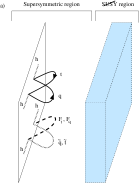
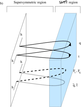
Figure 9: Loops near the brane (a) do not sense supersymmetry breaking and completely cancel. Only once the fields propagate far from the Yukawa brane (b) do they “notice” that supersymmetry is broken, for example by boundary conditions or localized supersymmetry breaking.

Calculating the diagram of Fig. 9, in momentum space for the usual four coordinates but in position space for the bulk, gives a Higgs mass-squared parameter:

$$m_{H}^{2}=-N_{c}f^{2}\int\!\!dy_{1}\,dy_{2}\,\delta(y_{1})\,\delta(y_{2})\int\!\!\frac{d^{4}k}{(2\pi)^{4}}\frac{1}{2}\left(\tilde{G}_{\psi}^{2}-\tilde{G}_{\phi}\tilde{G}_{F}\right).$$ (100)

The delta functions fix the Yukawa interactions on the brane at $y=0$, and the strength of the Yukawa coupling in 5d is $f=2\pi Ry_{t}$, as the Higgs is either a brane field or the zero mode of a bulk field. The propagators of the top-quark chiral multiplet, $\tilde{G}_{\phi,\psi,F}$ for scalar, fermion and $F$ components, are here normalized such that in a non-compactified fifth dimension $\tilde{G}_{\phi,\psi,F}=1$, giving an exact supersymmetric cancellation in Eq. (100). Since the delta functions force the propagators to start and finish at $y=0$, one might guess that they do not probe whether the space is compactified. This guess is incorrect: in a compactified space the propagation can wind $n$ times around the space (or reflect $n$ times), inducing $\tilde{G}_{\phi,\psi,F}=\tilde{G}_{\phi,\psi,F}(kR)$. The form of the $kR$ dependence is determined by how supersymmetry is broken and how $\phi,\psi$ and $F$ feel this breaking. In any theory in which there is no supersymmetry breaking locally near $y=0$, but rather has supersymmetry breaking on scales of order $\pi R$ from the Yukawa brane, then, for large $k$, $\tilde{G}_{\phi,\psi,F}=1+O(\exp(-k\pi R))$. This ensures the momentum integral gives a finite $O(1/(\pi R)^{4})$ result, so that $m_{H}^{2}\simeq-N_{c}\,y_{t}^{2}/(\pi^{4}R^{2})$. This general argument demonstrates that the physics of EWSB is strongly dominated by the scale $1/(\pi R)$ and is insensitive to how our 5d theory behaves when it becomes strongly coupled at larger energy scales.

In the models of sections 3 and 4, supersymmetric propagators have $\tilde{G}=\tanh[k\pi R]$, while those which feel supersymmetry breaking have $\tilde{G}=\coth[k\pi R]$. In both models the quark propagators are supersymmetric and the squark propagators feel supersymmetry breaking. The numerical difference in $m_{H}^{2}$ arises because in the Scherk-Schwarz theory the conjugate squarks (or $F$) propagator feels supersymmetry breaking, while in the case of a supersymmetry-breaking brane they do not.

Our new mechanism for radiative EWSB in the bulk has several important consequences for collider experiments. Since the higher dimensional theory possesses more supersymmetries than in 4d theories, there are more superpartners for particles which propagate in the bulk, which must include $t,b$ quarks and the standard-model gauge particles, and might include all matter. For example a top quark is accompanied by two scalar superpartners $\tilde{t}$ and $\tilde{t}^{c}$, as well as a fermionic superpartner $t^{c}$. All these superpartners lie in the TeV domain. Furthermore the superpartner masses are heavily influenced by the geometry of the bulk: all matter superpartners which propagate in the bulk, $\tilde{X}$, are highly degenerate, and similarly the conjugate matter superpartners, $\tilde{X}^{c}$, are all degenerate. This degeneracy implies that the flavor violation induced by squark or slepton exchange is mild, and not problematic as frequently encountered in 4d.

There are KK resonances for all standard-model particles which propagate in the bulk, and for all their superpartners. The mass spectra of these towers are regular with mass splittings $1/R$. Two simple examples of such spectra are shown in Figs. 2 and 6.

The Higgs sector of the theory is model dependent. For example the Higgs doublets and their superpartners might be bulk fields or reside on the brane where the Yukawa couplings are located. While a light Higgs frequently occurs, it is also easy to violate the upper bound on the lightest Higgs-boson mass of 4d supersymmetric theories. For example, the Higgs boson may evade this bound by radiative contributions to the effective potential of the Higgs from the KK tower of top quarks and squarks. A model where this occurs is given in section 5, where the Higgs mass is correlated with the compactification scale as shown in Fig. 7.

Two simple models discussed in this paper have unusual collider phenomenology. In one case the LSP is a top squark. In collider experiments this will lead to events with 1 or 2 highly ionizing charged tracks. In another case colored superpartners cascade decay to give Higgs bosons and gravitinos: $\tilde{g}\rightarrow\bar{q}q\tilde{h}$, followed by $\tilde{h}\rightarrow h\tilde{G}$, leading to remarkable events with two Higgs bosons, missing transverse energy and jets.

An important and generic consequence of our higher dimensional scheme for breaking weak interactions is that the superpartners are typically significantly heavier than in many 4d supersymmetric theories. In 4d theories the Higgs mass-squared parameter and the mass-squared parameters for squarks and sleptons occurs at the same order in perturbation theory. Color factors or careful parameter choices can push up the squark and slepton masses to some degree, but the expectation is that the masses will be at the scale of the electroweak vacuum expectation value. By contrast in our scheme matter superpartners acquire a tree-level mass from propagation in the bulk, while the Higgs mass-squared parameter is driven negative at the one-loop level. Superpartners which propagate in the bulk we find to be typically a loop factor of $\pi^{2}/2\simeq 5$ heavier than the mass scale of the radiatively generated Higgs mass. If all the superpartners propagate in the bulk, it is quite plausible that none will be lighter than 1 TeV.

References

- [1] R. Barbieri, S. Ferrara and C. A. Savoy, Phys. Lett. B119, 343 (1982); A. H. Chamseddine, R. Arnowitt and P. Nath, Phys. Rev. Lett. 49, 970 (1982); L. Hall, J. Lykken and S. Weinberg, Phys. Rev. D 27, 2359 (1983).
- [2] M. Dine and W. Fischler, Phys. Lett. B110, 227 (1982); L. Alvarez-Gaume, M. Claudson and M. B. Wise, Nucl. Phys. B207, 96 (1982).
- [3] LEP Electroweak Working Group, http://lepewwg.web.cern.ch/LEPEWWG/.
- [4] L. Ibanez and G. G. Ross, Phys. Lett. B110, 215 (1982); L. Alvarez-Gaume, J. Polchinski and M. B. Wise, Nucl. Phys. B221, 495 (1983); K. Inoue, A. Kakuto, H. Komatsu and S. Takeshita, Prog. Theor. Phys. 67, 1889 (1982); Prog. Theor. Phys. 68, 927 (1982).
- [5] Y. Okada, M. Yamaguchi and T. Yanagida, Prog. Theor. Phys. 85, 1 (1991); J. Ellis, G. Ridolfi and F. Zwirner, Phys. Lett. B257, 83 (1991); H. E. Haber and R. Hempfling, Phys. Rev. Lett. 66, 1815 (1991).
- [6] R. Barbieri and A. Strumia, hep-ph/0007265.
- [7] I. Antoniadis, Phys. Lett. B246, 377 (1990).
- [8] I. Antoniadis, C. Munoz and M. Quiros, Nucl. Phys. B397, 515 (1993) [hep-ph/9211309]; K. Benakli, Phys. Lett. B386, 106 (1996) [hep-th/9509115]; I. Antoniadis, S. Dimopoulos and G. Dvali, Nucl. Phys. B516, 70 (1998) [hep-ph/9710204].
- [9] A. Pomarol and M. Quiros, Phys. Lett. B438, 255 (1998) [hep-ph/9806263]; I. Antoniadis, S. Dimopoulos, A. Pomarol and M. Quiros, Nucl. Phys. B544, 503 (1999) [hep-ph/9810410]; A. Delgado, A. Pomarol and M. Quiros, Phys. Rev. D 60, 095008 (1999) [hep-ph/9812489].
- [10] I. Antoniadis and K. Benakli, Phys. Lett. B326, 69 (1994) [hep-th/9310151]; I. Antoniadis, K. Benakli and M. Quiros, Phys. Lett. B331, 313 (1994) [hep-ph/9403290]; Phys. Lett. B460, 176 (1999) [hep-ph/9905311]; E. Accomando, I. Antoniadis and K. Benakli, Nucl. Phys. B579, 3 (2000) [hep-ph/9912287]; P. Nath and M. Yamaguchi, Phys. Rev. D 60, 116004 (1999) [hep-ph/9902323]; Phys. Rev. D 60, 116006 (1999) [hep-ph/9903298]; P. Nath, Y. Yamada and M. Yamaguchi, Phys. Lett. B466, 100 (1999) [hep-ph/9905415]; W. J. Marciano, hep-ph/9902332; Phys. Rev. D 60, 093006 (1999) [hep-ph/9903451]; M. Masip and A. Pomarol, Phys. Rev. D 60, 096005 (1999) [hep-ph/9902467]; A. Delgado, A. Pomarol and M. Quiros, JHEP0001, 030 (2000) [hep-ph/9911252]; T. G. Rizzo and J. D. Wells, Phys. Rev. D 61, 016007 (2000) [hep-ph/9906234]; A. Strumia, Phys. Lett. B466, 107 (1999) [hep-ph/9906266]; R. Casalbuoni, S. De Curtis, D. Dominici and R. Gatto, Phys. Lett. B462, 48 (1999) [hep-ph/9907355]; C. D. Carone, Phys. Rev. D 61, 015008 (2000) [hep-ph/9907362].
- [11] R. Barbieri, L. J. Hall and Y. Nomura, hep-ph/0011311.
- [12] J. Scherk and J. H. Schwarz, Phys. Lett. B82, 60 (1979); Nucl. Phys. B153, 61 (1979); P. Fayet, Phys. Lett. B159, 121 (1985); Nucl. Phys. B263, 649 (1986).
- [13] N. Arkani-Hamed, Y. Grossman and M. Schmaltz, Phys. Rev. D 61, 115004 (2000) [hep-ph/9909411].
- [14] T. Appelquist, H. Cheng and B. A. Dobrescu, hep-ph/0012100.
- [15] Z. Chacko, M. A. Luty and E. Ponton, JHEP0007, 036 (2000) [hep-ph/9909248].
- [16] K. R. Dienes, E. Dudas and T. Gherghetta, Phys. Lett. B436, 55 (1998) [hep-ph/9803466]; Nucl. Phys. B537, 47 (1999) [hep-ph/9806292].
- [17] N. Arkani-Hamed, S. Dimopoulos and G. Dvali, Phys. Lett. B429, 263 (1998) [hep-ph/9803315]; Phys. Rev. D 59, 086004 (1999) [hep-ph/9807344]; I. Antoniadis, N. Arkani-Hamed, S. Dimopoulos and G. Dvali, Phys. Lett. B436, 257 (1998) [hep-ph/9804398].
- [18] N. Arkani-Hamed, L. Hall, D. Smith and N. Weiner, Phys. Rev. D 61, 116003 (2000) [hep-ph/9909326].