Light-cone distribution functions for $B$ decays
at subleading order in $1/m_{b}$

Abstract

We construct the higher twist structure functions that describe inclusive $b$ hadron decays in regions of phase space where the hadronic decay products carry high energy but have low invariant mass. We show that, for $B$ meson decays, there are four new non-vanishing matrix elements of non-local operators. We show that to subleading twist these decays are parametrized in terms of four functions. We compute the tree-level matching for a general heavy-to-light current and apply it to $\bar{B}\to X_{s}\gamma$. Using a simple model for these functions we estimate the subleading twist contributions to this decay.

I Introduction

Inclusive decays of $B$ mesons can be analyzed via an operator product expansion (OPE) [1] as a power series in $\Lambda_{\rm QCD}/m_{b}$. At leading order the OPE reproduces the parton model results, while non-perturbative physics is parametrized by matrix elements of higher dimensional operators and suppressed by powers of the heavy quark mass.

In practice, higher dimensional operators in the OPE are only suppressed for sufficiently inclusive observables. In the resonance regime, where the invariant mass of the final hadronic state is restricted to be $\mbox{\raisebox{-2.84526pt}{$\,\stackrel{{\scriptstyle<}}{{\scriptstyle\sim}}\,$}}\Lambda_{\rm QCD}^{2}$, the decay is no longer inclusive and it is not surprising that the OPE completely breaks down. However, the OPE includes terms suppressed by $E_{X}\Lambda_{\rm QCD}/m_{X}^{2}$ (where $E_{X}$ and $m_{X}$ are the energy and invariant mass of the final hadronic state) which are suppressed over most of phase space, but are $O(1)$ in the region of high energy, low invariant mass hadronic states,

$$E_{X}\sim m_{b},\ m_{X}^{2}\sim\Lambda_{\rm QCD}m_{b}\gg\Lambda_{\rm QCD}^{2}\,.$$ (1)

In this “shape function region” the OPE breaks down, even though it is far from the resonance regime. Thus an inclusive description is still appropriate, but the expansion parameter in the OPE has to be modified. It has been shown that the most singular terms in the OPE may be resummed into a non-local operator[2]

$$O_{0}(\omega)=\bar{h}_{v}\delta(\omega+in\cdot\hat{D})h_{v}\,,$$ (2)

where $n^{\mu}$ is a light-like vector in the direction of the final hadrons, $h_{v}$ is a HQET heavy quark field and we denote variables normalized to $m_{b}$ by a hat: $\hat{D}^{\mu}\equiv D^{\mu}/m_{b}$. The matrix element of this operator in a $B$ meson is the light-cone structure function of the meson,

$$f(\omega)={1\over 2m_{B}}\langle B|O_{0}(\omega)|B\rangle\,.$$ (3)

The rate in the shape function region is determined by $f(\omega)$. However, since it is a non-perturbative function, $f(\omega)$ cannot be calculated analytically, and the rate in the shape function region is model-dependent even at leading order in $\Lambda_{\rm QCD}/m_{b}$.

Unfortunately, for $\bar{B}\rightarrow X_{u}\ell\bar{\nu}$ decay (and to a lesser extent $\bar{B}\rightarrow X_{s}\gamma$), the experimental cuts which must be imposed on the phase space to eliminate large backgrounds from $b\rightarrow c$ decay typically put the decay into the shape function region, introducing large model-dependence in the predicted rate. For semileptonic $b\rightarrow u$ decay, this is the case for cuts on either the charged lepton energy or the hadronic invariant mass[3], and this model dependence is the major theoretical stumbling block to a precise determination of the CKM matrix element $|V_{ub}|$ from inclusive decays.

However, since the distribution function (3) determines the shape of the photon spectrum in $\bar{B}\rightarrow X_{s}\gamma$ as well as the charged lepton or hadronic invariant mass spectrum in $\bar{B}\rightarrow X_{u}\ell\bar{\nu}$, it was suggested a number of years ago[4] that $f(y)$ could be measured in $\bar{B}\rightarrow X_{s}\gamma$, and then used to extract $|V_{ub}|$ from semileptonic decay. The perturbative corrections to the relation between these processes have been intensely studied in recent years[6].

In addition to the radiative corrections, however, there are non-perturbative corrections to the relation between the photon spectrum in $\bar{B}\rightarrow X_{s}\gamma$ and the lepton or hadronic invariant mass spectra in $\bar{B}\rightarrow X_{u}\ell\bar{\nu}$. The light-cone distribution function (3) only resums the most singular terms of the OPE in the shape function region. There are corrections to this from less singular terms suppressed by $\Lambda_{\rm QCD}/m_{b}$, analogous to higher-twist corrections to deep inelastic scattering [7]. These corrections are important for a precision measurement of $|V_{ub}|$ via this method, but have not yet been studied.

In this paper we discuss the subleading corrections to heavy-light $B$ decay in the shape function region by performing a twist expansion rather than the usual OPE in terms of local operators. At leading order in the twist expansion we reproduce the known results, while at subleading order we find four new non-local operators relevant for $B$ decays. We compute the tree-level matching for a general heavy-light current and apply it to $\bar{B}\rightarrow X_{s}\gamma$, reserving a discussion of $\bar{B}\rightarrow X_{u}\ell\bar{\nu}$ decay for a future work[9]. We use a simple model for these functions to estimate the subleading twist contribution to $B\rightarrow X_{s}\gamma$.

II Kinematics

We consider a general heavy to light transition (radiative or semileptonic), proceeding via the current

$$j(x)=\bar{q}(x)\Gamma b(x),$$ (4)

where $q(x)$ is a massless quark field and $\Gamma$ is an arbitrary Dirac matrix. The decay rate is related to the imaginary part of the $T$-product of two heavy-light currents:

$$d\Gamma\sim-2\,{\rm Im}\,\langle B|{\cal T}|B\rangle\,,$$ (5)

where

$${\cal T}(q)=\int\!d^{4}x\,T\left[j(0)j^{\dagger}(x)\right]e^{iqx}\,,$$ (6)

and $q$ is the momentum transfer.

The kinematics for this process are shown in Fig. 1.

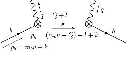
FIG. 1.: Kinematics for a general heavy to light transition.

As usual, the heavy quark momentum is split into a large and a residual piece, $p_{b}^{\mu}=m_{b}v^{\mu}+k^{\mu}$. In the shape function region the final hadronic state has large energy but small invariant mass, and so its momentum lies close to the light-cone. We introduce a light-like vector $n^{\mu}$ to define the expansion of the jet about the light-cone, and the velocity of the heavy quark then defines a second light-like vector $\bar{n}=2v-n$. These vectors satisfy

$$n^{2}=0=\bar{n}^{2},\quad v\cdot n=v\cdot\bar{n}=1,\quad n\cdot\bar{n}=2.$$ (7)

In the frame in which the $b$ quark is at rest and the emitted hadrons move in the $+z$ direction, these vectors are given by $n^{\mu}=(1,0,0,1)$, $\bar{n}^{\mu}=(1,0,0,-1)$ and $v^{\mu}=(1,0,0,0)$. We can decompose the metric according to

$$g^{\mu\nu}=\frac{1}{2}\left(n^{\mu}\bar{n}^{\nu}+n^{\nu}\bar{n}^{\mu}\right)+g^{\mu\nu}_{\perp}\,,$$ (8)

which defines $g^{\mu\nu}_{\perp}$.

In the shape function region, the momenta scale as

$$(m_{b}v-q)\cdot\bar{n} = m_{b}-q\cdot\bar{n}\sim O(m_{b}),$$ (9)

$$(m_{b}v-q)\cdot n = m_{b}-q\cdot n\sim O(\Lambda_{\rm QCD}),$$ (10)

$$k^{\mu} \sim O(\Lambda_{\rm QCD}).$$ (11)

It is therefore convenient to split the momentum $q^{\mu}$ into large and small components,

$$q^{\mu}\equiv Q^{\mu}+\ell^{\mu}\,,$$ (12)

where

$$Q^{\mu}={\textstyle{1\over 2}}(m_{b}\bar{n}^{\mu}+q\cdot\bar{n}n^{\mu}),\ \ \ \ell^{\mu}=-{\textstyle{1\over 2}}(m_{b}-q\cdot n)\bar{n}^{\mu}$$ (13)

are $O(m_{b})$ and $O(\Lambda_{\rm QCD})$, respectively. The momentum of the light hadronic decay products is

$$p_{q}^{\mu}=m_{b}v^{\mu}-Q^{\mu}-\ell^{\mu}+k^{\mu}={\textstyle{1\over 2}}(m_{b}-q\cdot\bar{n})n^{\mu}+{\textstyle{1\over 2}}(m_{b}-q\cdot n)\bar{n}^{\mu}+k^{\mu}\,,$$ (14)

and so in the shape function region (9) we have $p_{q}^{2}={\cal O}(\Lambda_{\rm QCD}m_{b})\ll m_{b}^{2}$.

III Matching

A Leading Order

The expansion in the shape function region differs from the usual $1/m_{b}$ expansion because of the additional small parameter $m_{b}-q\cdot n$; in the usual OPE terms of order

$${k^{\mu}\over m_{b}-q\cdot n}$$

are treated as subleading, whereas they are $O(1)$ in the shape function region. Thus, instead of resumming terms of this form to all orders, we perform an OPE in powers of $\Lambda_{\rm QCD}/m_{b}$, but using the scaling (9). This is analogous to the twist expansion in DIS.

Expanding the light-quark propagator shown in Fig. 1 in powers of $\Lambda_{\rm QCD}/m_{b}$ gives

$${m_{b}\mathchoice{\ooalign{$\hfil\displaystyle\mkern 0.0mu/\hfil$\crcr$\displaystyle v$}}{\ooalign{$\hfil\textstyle\mkern 0.0mu/\hfil$\crcr$\textstyle v$}}{\ooalign{$\hfil\scriptstyle\mkern 0.0mu/\hfil$\crcr$\scriptstyle v$}}{\ooalign{$\hfil\scriptscriptstyle\mkern 0.0mu/\hfil$\crcr$\scriptscriptstyle v$}}+\mathchoice{\ooalign{$\hfil\displaystyle\mkern 0.0mu/\hfil$\crcr$\displaystyle k$}}{\ooalign{$\hfil\textstyle\mkern 0.0mu/\hfil$\crcr$\textstyle k$}}{\ooalign{$\hfil\scriptstyle\mkern 0.0mu/\hfil$\crcr$\scriptstyle k$}}{\ooalign{$\hfil\scriptscriptstyle\mkern 0.0mu/\hfil$\crcr$\scriptscriptstyle k$}}-\mathchoice{\ooalign{$\hfil\displaystyle\mkern 0.0mu/\hfil$\crcr$\displaystyle Q$}}{\ooalign{$\hfil\textstyle\mkern 0.0mu/\hfil$\crcr$\textstyle Q$}}{\ooalign{$\hfil\scriptstyle\mkern 0.0mu/\hfil$\crcr$\scriptstyle Q$}}{\ooalign{$\hfil\scriptscriptstyle\mkern 0.0mu/\hfil$\crcr$\scriptscriptstyle Q$}}-\mathchoice{\ooalign{$\hfil\displaystyle\mkern 0.0mu/\hfil$\crcr$\displaystyle l$}}{\ooalign{$\hfil\textstyle\mkern 0.0mu/\hfil$\crcr$\textstyle l$}}{\ooalign{$\hfil\scriptstyle\mkern 0.0mu/\hfil$\crcr$\scriptstyle l$}}{\ooalign{$\hfil\scriptscriptstyle\mkern 0.0mu/\hfil$\crcr$\scriptscriptstyle l$}}\over\left(m_{b}v+k-Q-l+i\epsilon\right)^{2}}={1\over 2}\,{\mathchoice{\ooalign{$\hfil\displaystyle\mkern 0.0mu/\hfil$\crcr$\displaystyle n$}}{\ooalign{$\hfil\textstyle\mkern 0.0mu/\hfil$\crcr$\textstyle n$}}{\ooalign{$\hfil\scriptstyle\mkern 0.0mu/\hfil$\crcr$\scriptstyle n$}}{\ooalign{$\hfil\scriptscriptstyle\mkern 0.0mu/\hfil$\crcr$\scriptscriptstyle n$}}\over m_{b}-q\cdot n+k\cdot n+i\epsilon}+O\left({\Lambda_{\rm QCD}\over m_{b}}\right).$$ (15)

Since $k\cdot n$ and $m_{b}-q\cdot n$ are of the same order, this term cannot be expanded in powers of $k\cdot n$, and so cannot be matched onto a finite set of local operators.

Instead, consider the set of operators

$$\tilde{O}_{0}(t)=\bar{h}_{v}(0)E(0,t)h_{v}(t)\,,$$ (16)

where we use the shorthand notation

$$\psi(t)\equiv\psi\left({nt}\over m_{b}\right),$$ (17)

where $t$ is dimensionless, to denote fields on the light-cone defined by $n^{\mu}$. The path-ordered exponential

$$E(t_{1},t_{2})=P\exp\left(-i\int_{t_{1}}^{t_{2}}n\cdot\hat{A}(t^{\prime})\,dt^{\prime}\right)$$ (18)

is required to make the operator $\tilde{O}_{0}(t)$ gauge invariant. The operators $O_{0}(\omega)$ are defined in terms of $\tilde{O}_{0}(t)$ by the linear combination

$$O_{0}(\omega)={1\over 2\pi}\int_{-\infty}^{\infty}dt\,e^{-i\omega t}O_{0}(t)=\bar{h}_{v}\delta(\omega+in\cdot\hat{D})h_{v}\,,$$ (19)

and have the required form for the imaginary part of the leading term in the heavy quark expansion (15). The matrix elements of $O_{0}(\omega)$ define the light-cone distribution function of the $b$ quark in a $B$ meson

$$f(\omega)\equiv{1\over 2m_{B}}\langle B|\bar{h}_{v}\delta(\omega+in\cdot\hat{D})h_{v}|B\rangle\,.$$ (20)

Expanding $f(\omega)$ in powers of $in\cdot\hat{D}$ gives the series of increasingly singular terms

$$f(\omega)=\delta(\omega)-\frac{\lambda_{1}}{6m_{b}^{2}}\delta^{\prime\prime}(\omega)-\frac{\rho_{1}}{18m_{b}^{3}}\delta^{\prime\prime\prime}(\omega)+\cdots\\$$ (21)

where

$${1\over 2m_{B}}\langle B|\bar{h}_{v}(iD_{\alpha})(iD_{\beta})h_{v}|B\rangle \equiv {1\over 3}(g_{\alpha\beta}-v_{\alpha}v_{\beta})\lambda_{1}$$ (22)

$${1\over 2m_{B}}\langle B|(iD_{\alpha})(iD_{\mu})(iD_{\beta})|B\rangle \equiv {1\over 3}(g_{\alpha\beta}-v_{\alpha}v_{\beta})v_{\mu}\rho_{1}.$$ (23)

For a general $b$ hadron decay there is an additional parity-odd operator at leading twist

$$\tilde{P}_{0}^{\alpha}(t)=\bar{h}_{v}(0)\gamma^{\alpha}\gamma_{5}E(0,t)h_{v}(t)\,,$$ (24)

whith $P_{0}^{\alpha}(\omega)$ defined analogously to (19). This operator is not relevant for $B$ meson decays since its matrix element vanishes, but it gives a spin dependent contribution to $\Lambda_{b}$ decay. A general Dirac structure between heavy quark fields may be expressed in terms of these four independent matrices via the projection formula

$$P_{+}\Gamma P_{+}=\frac{1}{2}P_{+}{\rm Tr}(P_{+}\Gamma)-\frac{1}{2}s_{\mu}{\rm Tr}(s^{\mu}\Gamma)\,,$$ (25)

where

$$s_{\mu}\equiv P_{+}\gamma_{\mu}\gamma_{5}P_{+}\,,$$ (26)

and $P_{+}\equiv\frac{1}{2}(1+\mathchoice{\ooalign{$\hfil\displaystyle\mkern 0.0mu/\hfil$\crcr$\displaystyle v$}}{\ooalign{$\hfil\textstyle\mkern 0.0mu/\hfil$\crcr$\textstyle v$}}{\ooalign{$\hfil\scriptstyle\mkern 0.0mu/\hfil$\crcr$\scriptstyle v$}}{\ooalign{$\hfil\scriptscriptstyle\mkern 0.0mu/\hfil$\crcr$\scriptscriptstyle v$}})$.

Since the OPE is performed over a a continuously infinite set of operators labeled by $\omega$, the heavy quark expansion in the shape function region is, like in DIS, a convolution over a single parameter which may be interpreted as the light-cone momentum fraction of the heavy quark:

$${\rm Im}\,{\cal T}(q)=-{1\over 2m_{b}}\int_{-\infty}^{\infty}\!d\omega\,\left[C_{0}(\omega)O_{0}(\omega)+C_{5,0}^{\alpha}(\omega)P_{0,\alpha}(\omega)+O\left({\Lambda_{\rm QCD}\over m_{b}}\right)\right]\,,$$ (27)

where the $C_{i}$’s are perturbatively calculable short distance coefficients. The tree level matching conditions are easily obtained from (15) and (25):

$$C_{0}(v,q,\omega) = \frac{\pi}{2}{\rm Tr}\left(P_{+}\Gamma n\!\!\!/\overline{\Gamma}\right)\delta(1-n\cdot\hat{q}-\omega)$$ (28)

$$C_{5,0}^{\alpha}(v,q,\omega) = -\frac{\pi}{2}{\rm Tr}\left(s^{\alpha}\Gamma n\!\!\!/\overline{\Gamma}\right)\delta(1-n\cdot\hat{q}-\omega)\,.$$ (29)

B Subleading Order

Expanding (15) to subleading order in $1/m_{b}$, we will in general match onto non-local objects of the form[7]

$$\tilde{O}_{\Gamma}^{\mu_{1}\dots\mu_{n-1}}(t_{1},\dots,t_{n})=\bar{h}_{v}(0)\Gamma\big{[}iD^{\mu_{1}}(t_{1})\dots iD^{\mu_{n-1}}(t_{n-1})\big{]}h_{v}(t_{n})\,,$$ (30)

where $\Gamma=1$ or $\gamma_{\alpha}\gamma_{5}$ and

$$D_{\mu}(t)\equiv\partial_{\mu}-igA_{\mu}^{a}(t)T^{a}$$ (31)

is the usual covariant derivative, acting at a light-cone coordinate.

The most general case involves operators in which every field and derivative is evaluated at a different light-cone coordinate. However for heavy quark decays to subleading order, we find that at maximum only two light-cone coordinates enter. The complete set of operators required is:

$$\tilde{O}_{1}^{\mu}(t) = \bar{h}_{v}(0)\left(-i\raise 6.45831pt\hbox{$\leftarrow$}\mkern-16.5muD^{\mu}(0)E(0,t)+E(0,t)iD^{\mu}(t)\right)h_{v}(t)$$ (32)

$$\tilde{P}_{1,\alpha}^{\mu}(t) = \bar{h}_{v}(0)\left(-i\raise 6.45831pt\hbox{$\leftarrow$}\mkern-16.5muD^{\mu}(0)E(0,t)+E(0,t)iD^{\mu}(t)\right)\gamma_{\alpha}\gamma_{5}h_{v}(t)$$ (33)

$$\tilde{O}_{2}^{\mu}(t) = i\bar{h}_{v}(0)\left(-i\raise 6.45831pt\hbox{$\leftarrow$}\mkern-16.5muD^{\mu}(0)E(0,t)-E(0,t)iD^{\mu}(t)\right)h_{v}(t)$$ (34)

$$\tilde{P}_{2,\alpha}^{\mu}(t) = i\bar{h}_{v}(0)\left(-i\raise 6.45831pt\hbox{$\leftarrow$}\mkern-16.5muD^{\mu}(0)E(0,t)-E(0,t)iD^{\mu}(t)\right)\gamma_{\alpha}\gamma_{5}h_{v}(t)$$ (35)

$$\tilde{O}_{3}^{\mu\nu}(t_{1},t_{2}) = \bar{h}_{v}(0)E(0,t_{1})\left\{iD_{\perp}^{\mu}(t_{1}),iD_{\perp}^{\nu}(t_{1})\right\}E(t_{1},t_{2})h_{v}(t_{2})$$ (36)

$$\tilde{P}_{3,\alpha}^{\mu\nu}(t_{1},t_{2}) = \bar{h}_{v}(0)E(0,t_{1})\left\{iD_{\perp}^{\mu}(t_{1}),iD_{\perp}^{\nu}(t_{1})\right\}E(t_{1},t_{2})\gamma_{\alpha}\gamma_{5}h_{v}(t_{2})$$ (37)

$$\tilde{O}_{4}^{\mu\nu}(t_{1},t_{2}) = g\bar{h}_{v}(0)E(0,t_{1})G^{\mu\nu}_{\perp}(t_{1})E(t_{1},t_{2})h_{v}(t_{2})$$ (38)

$$\tilde{P}_{4,\alpha}^{\mu\nu}(t_{1},t_{2}) = g\bar{h}_{v}(0)E(0,t_{1})G^{\mu\nu}_{\perp}(t_{1})E(t_{1},t_{2})\gamma_{\alpha}\gamma_{5}h_{v}(t_{2})\,,$$ (39)

where $D_{\perp}^{\mu}=g^{\mu\nu}_{\perp}D_{\nu}$ and $g\,G^{\mu\nu}_{\perp}=i[(iD^{\mu}_{\perp}),(iD^{\nu}_{\perp})]$ is the gluon field strength.

The Fourier transformed operators $O_{i}$ are defined as

$$O_{1}^{\mu}(\omega) = {1\over 2\pi}\int_{-\infty}^{\infty}dt\,e^{-i\omega t}\tilde{O}_{1}^{\mu}(t)=\bar{h}_{v}\left\{iD^{\mu},\delta(in\cdot\hat{D}+\omega)\right\}h_{v}$$ (40)

$$O_{2}^{\mu}(\omega) = {1\over 2\pi}\int_{-\infty}^{\infty}dt\,e^{-i\omega t}\tilde{O}_{2}^{\mu}(t)=i\bar{h}_{v}\left[iD^{\mu},\delta(in\cdot\hat{D}+\omega)\right]h_{v}$$ (41)

$$O_{3}^{\mu\nu}(\omega_{1},\omega_{2}) = \left({1\over 2\pi}\right)^{2}\int_{-\infty}^{\infty}dt_{1}\,dt_{2}\,e^{-i\omega_{1}t_{1}}e^{-i(\omega_{1}-\omega_{2})t_{2}}\tilde{O}_{3}^{\mu\nu}(t_{1},t_{2})$$ (42)

$$= \bar{h}_{v}\delta(in\cdot\hat{D}+\omega_{2})\left\{iD^{\mu}_{\perp},iD^{\nu}_{\perp}\right\}\delta(in\cdot\hat{D}+\omega_{1})h_{v}$$ (43)

$$O_{4}^{\mu\nu}(\omega_{1},\omega_{2}) = \left({1\over 2\pi}\right)\int_{-\infty}^{\infty}dt_{1}\,dt_{2}\,e^{-i\omega_{1}t_{1}}e^{-i(\omega_{1}-\omega_{2})t_{2}}\tilde{O}_{4}^{\mu\nu}(t_{1},t_{2})$$ (44)

$$= g\bar{h}_{v}\delta(in\cdot\hat{D}+\omega_{2})G_{\perp}^{\mu\nu}\delta(in\cdot\hat{D}+\omega_{1})h_{v}\,.$$ (45)

Similarly the Fourier transforms of the $\tilde{P}_{i}$’s are

$$P_{1,\alpha}^{\mu}(\omega) = \bar{h}_{v}\left\{iD^{\mu},\delta(in\cdot\hat{D}+\omega)\right\}\gamma_{\alpha}\gamma_{5}h_{v}$$ (46)

$$P_{2,\alpha}^{\mu}(\omega) = i\bar{h}_{v}\left[iD^{\mu},\delta(in\cdot\hat{D}+\omega)\right]\gamma_{\alpha}\gamma_{5}h_{v}$$ (47)

$$P_{3,\alpha}^{\mu\nu}(\omega_{1},\omega_{2}) = \bar{h}_{v}\delta(in\cdot\hat{D}+\omega_{2})\left\{iD^{\mu}_{\perp},iD^{\nu}_{\perp}\right\}\delta(in\cdot\hat{D}+\omega_{1})\gamma_{\alpha}\gamma_{5}h_{v}$$ (48)

$$P_{4,\alpha}^{\mu\nu}(\omega_{1},\omega_{2}) = g\bar{h}_{v}\delta(in\cdot\hat{D}+\omega_{2})G_{\perp}^{\mu\nu}\delta(in\cdot\hat{D}+\omega_{1})\gamma_{\alpha}\gamma_{5}h_{v}.$$ (49)

The Feynman rules for the operators $O_{0}-O_{4}$ in $n\cdot A=0$ gauge are shown in Fig. 2.

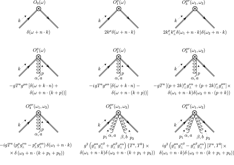
FIG. 2.: Feynman rules for non-local operators $O_{0}-O_{4}$ in $n\cdot A=0$ gauge. The Feynman rules for $P_{0}-P_{4}$ are identical except for the Dirac structure.

Finally, at subleading order there are also contributions from the time-ordered products of $O_{0}(\omega)$ with the subleading terms in the HQET Lagrangian,

$${\cal O}_{1/m}(y)=\bar{h}_{v}(y)(iD)^{2}h_{v}(y)+{g\over 2}\bar{h}_{v}(y)\sigma_{\mu\nu}G^{\mu\nu}h_{v}(y)\,.$$ (50)

This yields another two operators

$$O_{T}(\omega) = i\int\!d^{4}y\,\frac{1}{2\pi}\int\!dt\,e^{-i\omega t}T\left(\bar{h}_{v}(0)h_{v}(t){\cal O}_{1/m}(y)\right)$$ (51)

$$P_{T,\alpha}(\omega) = i\int\!d^{4}y\,\frac{1}{2\pi}\int\!dt\,e^{-i\omega t}T\left(\bar{h}_{v}(0)\gamma_{\alpha}\gamma_{5}h_{v}(t){\cal O}_{1/m}(y)\right)\,.$$ (52)

At subleading order the nonlocal OPE in (27) is

$$-2m_{b}\,{\rm Im}\,{\cal T}(q) = \vphantom{{\Lambda_{\rm QCD}^{2}\over m_{b}^{2}}}\int\!d\omega\,\left(C_{0}(v,q,\omega)O_{0}(\omega)+C_{5,0}^{\alpha}(v,q,\omega)P_{0,\alpha}(\omega)\right)$$ (58)

$$\qquad+\frac{1}{2m_{b}}\sum_{i=1,2}\int\!d\omega\,\left(C_{i}^{\mu}(v,q,\omega)O_{i,\mu}(\omega)+C_{5,i}^{\alpha,\mu}(v,q,\omega)P_{i,\alpha,\mu}(\omega)\right)$$

$$\qquad+\frac{1}{2m_{b}}\sum_{i=3,4}\int\!d\omega_{1}d\omega_{2}\,\left(C_{i}^{\mu\nu}(v,q,\omega_{1},\omega_{2})O_{i,\mu\nu}(\omega_{1},\omega_{2})\right.$$

$$\qquad\qquad\qquad\qquad\left.+C_{5,i}^{\alpha,\mu\nu}(v,q,\omega_{1},\omega_{2})P_{i,\alpha,\mu\nu}(\omega_{1},\omega_{2})\right)$$

$$\qquad+\frac{1}{2m_{b}}\int\!d\omega\,\left(C_{T}(v,q,\omega)O_{T}(\omega)+C_{5,T}^{\alpha}(v,q,\omega)P_{T,\alpha}(\omega)\right)$$

$$\qquad+O\left({\Lambda_{\rm QCD}^{2}\over m_{b}^{2}}\right)\,.$$

The matching at subleading order onto the operators (32) is performed by computing the zero, one and two gluon matrix elements of (6) in full QCD and comparing this to the operators in (40) and (46). Note that this includes terms from the expansion of the $b$ quark field,

$$b=\left(1+{i\mathchoice{\ooalign{$\hfil\displaystyle\mkern 0.0mu/\hfil$\crcr$\displaystyle D$}}{\ooalign{$\hfil\textstyle\mkern 0.0mu/\hfil$\crcr$\textstyle D$}}{\ooalign{$\hfil\scriptstyle\mkern 0.0mu/\hfil$\crcr$\scriptstyle D$}}{\ooalign{$\hfil\scriptscriptstyle\mkern 0.0mu/\hfil$\crcr$\scriptscriptstyle D$}}\over{2m_{b}}}+\dots\right)h_{v}.$$ (59)

At tree level, we find

$$C_{1}^{\mu}(v,q,\omega) = \frac{\pi}{4}{\rm Tr}\left(\{P_{+},\gamma^{\mu}\}\Gamma n\!\!\!/\overline{\Gamma}\right)\delta(1-n\cdot\hat{q}-\omega)$$ (60)

$$C_{2}^{\mu}(v,q,\omega) = (-i)\frac{\pi}{4}{\rm Tr}\left([P_{+},\gamma^{\mu}]\Gamma n\!\!\!/\overline{\Gamma}\right)\delta(1-n\cdot\hat{q}-\omega)$$ (61)

$$C_{3}^{\mu\nu}(v,q,\omega_{1},\omega_{2}) = -\frac{\pi}{2}g_{\perp}^{\mu\nu}\frac{1}{m_{b}-\bar{n}\cdot q}{\rm Tr}\left(P_{+}\Gamma n\!\!\!/\overline{\Gamma}\right)$$ (63)

$$\qquad\times\left(\frac{\delta(1-n\cdot\hat{q}-\omega_{1})-\delta(1-n\cdot\hat{q}-\omega_{2})}{\omega_{1}-\omega_{2}}\right)$$

$$C_{4}^{\mu\nu}(v,q,\omega_{1},\omega_{2}) = i\,\frac{\pi}{2}\frac{1}{m_{b}-\bar{n}\cdot q}{\rm Tr}\left(P_{+}\Gamma n\!\!\!/(-i\sigma_{\!\!\perp}^{\mu\nu})\overline{\Gamma}\right)$$ (65)

$$\qquad\times\left(\frac{\delta(1-n\cdot\hat{q}-\omega_{1})-\delta(1-n\cdot\hat{q}-\omega_{2})}{\omega_{1}-\omega_{2}}\right)$$

$$C_{T}(n\cdot q,\omega) = C_{0}(n\cdot q,\omega)\,,$$ (66)

and for the corresponding spin dependent operators

$$C_{5,1}^{\alpha,\mu}(v,q,\omega) = -\frac{\pi}{4}{\rm Tr}\left(\{s^{\alpha},\gamma^{\mu}\}\Gamma n\!\!\!/\overline{\Gamma}\right)\delta(1-n\cdot\hat{q}-\omega)$$ (67)

$$C_{5,2}^{\alpha,\mu}(v,q,\omega) = i\,\frac{\pi}{4}{\rm Tr}\left([s^{\alpha},\gamma^{\mu}]\Gamma n\!\!\!/\overline{\Gamma}\right)\delta(1-n\cdot\hat{q}-\omega)$$ (68)

$$C_{5,3}^{\alpha,\mu\nu}(v,q,\omega_{1},\omega_{2}) = \frac{\pi}{2}g_{\perp}^{\mu\nu}\frac{1}{m_{b}-\bar{n}\cdot q}{\rm Tr}\left(s^{\alpha}\Gamma n\!\!\!/\overline{\Gamma}\right)$$ (70)

$$\qquad\times\left(\frac{\delta(1-n\cdot\hat{q}-\omega_{1})-\delta(1-n\cdot\hat{q}-\omega_{2})}{\omega_{1}-\omega_{2}}\right)$$

$$C_{5,4}^{\alpha,\mu\nu}(n\cdot q,\omega_{1},\omega_{2}) = (-i)\frac{\pi}{2}\frac{1}{m_{b}-\bar{n}\cdot q}{\rm Tr}\left(s^{\alpha}\Gamma n\!\!\!/(-i\sigma_{\!\!\perp}^{\mu\nu})\overline{\Gamma}\right)$$ (72)

$$\qquad\times\left(\frac{\delta(1-n\cdot\hat{q}-\omega_{1})-\delta(1-n\cdot\hat{q}-\omega_{2})}{\omega_{1}-\omega_{2}}\right)$$

$$C_{5,T}^{\alpha}(n\cdot q,\omega) = C_{5,0}^{\alpha}(n\cdot q,\omega)\,.$$ (73)

IV Matrix Elements

Matrix elements of the subleading operators (40), (46) and (51) give rise to new, subleading structure functions. Writing the most general Ansatz consistent with the symmetries and the equation of motion $(iv\cdot D)\,h=0$, we find that only the following matrix elements are non-vanishing

$$\langle B(v)|O_{1}^{\mu}(\omega)|B(v)\rangle = 2m_{B}\,g_{1}(\omega)(v^{\mu}-n^{\mu})$$ (74)

$$\langle B(v)|O_{3}^{\mu\nu}(\omega_{1},\omega_{2})|B(v)\rangle = 2m_{B}\,g_{2}(\omega_{1},\omega_{2})g_{\perp}^{\mu\nu}$$ (75)

$$\langle B(v)|P_{2,\alpha}^{\mu}(\omega)|B(v)\rangle = 2m_{B}\,h_{1}(\omega)\varepsilon_{\perp,\alpha}^{\mu}$$ (76)

$$\langle B(v)|P_{4,\alpha}^{\mu\nu}(\omega_{1},\omega_{2})|B(v)\rangle = 2m_{B}\,h_{2}(\omega_{1},\omega_{2})\varepsilon_{\rho\sigma\alpha\beta}\,g_{\perp}^{\mu\rho}g_{\perp}^{\nu\sigma}v^{\beta}$$ (77)

$$\langle B(v)|O_{T}(\omega)|B(v)\rangle = 2m_{B}\,t(\omega)\,,$$ (78)

where we define

$$\varepsilon_{\perp}^{\mu\nu}=\varepsilon^{\mu\nu\alpha\beta}v_{\alpha}n_{\beta}\,,$$ (79)

and $\varepsilon^{0123}=1$.

The matrix element of $O_{4}^{\mu\nu}(\omega_{1},\omega_{2})$ between $B$ mesons vanishes since no antisymmetric, parity even object can be constructed which is perpendicular to both $v$ and $n$. Similarly, the matrix element of $P_{3,\alpha}^{\mu\nu}(\omega_{1},\omega_{2})$ vanishes, since there is no parity odd, symmetric object perpendicular to $v$ and $n$. Due to the equations of motion, the matrix element of $O_{2}^{\mu}(\omega)$ must be proportional to $(v^{\mu}-n^{\mu})$:

$$\langle B(v)|O_{2}^{\mu}(\omega)B(v)\rangle=a(v^{\mu}-n^{\mu})\,.$$ (80)

Contracting with $n^{\mu}$ we find

$$a=\langle B(v)|n\cdot O_{2}(\omega)|B(v)\rangle=\langle B(v)|i\bar{h}_{v}\big{[}in\cdot D,\delta(in\cdot\hat{D}+\omega)\big{]}h_{v}|B(v)\rangle=0\,,$$ (81)

(where the last equality is due to the delta function) and so the matrix element vanishes. The matrix element of $P_{1,\alpha}^{\mu}(\omega)$ vanishes since all of its moments with respect to $\omega$ vanish. Finally, the matrix element of $P_{T,\alpha}(\omega)$ vanishes due to parity.

There is additional information on the remaining new functions. Starting with $g_{1}(\omega)$, we find

$$2m_{B}g_{1}(\omega) = n_{\mu}\langle B(v)|O_{1}^{\mu}(\omega)|B(v)\rangle=\langle B(v)|\bar{h}_{v}\left\{in\cdot D,\delta(in\cdot\hat{D}+\omega)\right\}h_{v}|B(v)\rangle$$ (82)

$$= -2(m_{b}\,\omega)\langle B(v)|\bar{h}_{v}\delta(i\hat{D}\cdot n+\omega)h_{v}|B(v)\rangle=-4m_{B}(m_{b}\,\omega)\,f(\omega)\,.$$ (83)

Thus, $g_{1}(\omega)$ is determined by the leading order structure function, $g_{1}(\omega)=-2(m_{b}\,\omega)\,f(\omega)$. Some information can also be obtained on moments of the function $g_{2}(\omega_{1},\omega_{2})$:

$$g_{2}^{(m,n)} = (-1)^{m+n}\int\!d\omega_{1}d\omega_{2}\omega_{1}^{n}\omega_{2}^{m}g_{2}(\omega_{1},\omega_{2})$$ (84)

$$= \frac{1}{2m_{B}}\langle B(v)|\bar{h}_{v}(in\cdot D)^{m}(iD_{\perp})^{2}(in\cdot D)^{n}h_{v}|B(v)\rangle\,,$$ (85)

leading to

$$g_{2}^{(0,0)} = \frac{2\lambda_{1}}{3}\,,$$ (86)

$$g_{2}^{(m,0)} = g_{2}^{(0,n)}=0\,,\qquad m,n\not=0\,,$$ (87)

where the last equality arises because of the constraints from the equations of motion [10]

$$\langle B|\bar{h}_{v}(iD_{\alpha})(iD_{\nu_{1}})\dots(iD_{\nu_{n}})(iD_{\beta})h_{v}|B\rangle=(g_{\alpha\beta}-v_{\alpha}v_{\beta}){\cal A}_{\nu_{1}\dots\nu_{n}}.$$ (88)

We can also obtain information on the parity odd operators. The function $h_{1}(\omega)$ is a genuine new non-perturbative function which introduces spin dependent effects. The first three moments of this function are given by

$$\int\!d\omega\,h_{1}(\omega)=0\,;\qquad\int\!d\omega\,\omega\,h_{1}(\omega)=-\frac{\lambda_{2}}{m_{b}}\,;\qquad\int\!d\omega\,\omega^{2}h_{1}(\omega)=\frac{\rho_{2}}{m_{b}^{2}}\,\,$$ (89)

where

$${1\over 2m_{B}}\langle B|\bar{h}_{v}(iD_{\alpha})(iD_{\beta})s_{\lambda}h_{v}|B\rangle \equiv {1\over 2}i\epsilon_{\nu\alpha\beta\lambda}v^{\nu}\lambda_{2}$$ (90)

$${1\over 2m_{B}}\langle B|\bar{h}_{v}(iD_{\alpha})(iD_{\mu})(iD_{\beta})s_{\lambda}h_{v}|B\rangle \equiv {1\over 2}i\epsilon_{\nu\alpha\beta\lambda}v^{\nu}v_{\mu}\rho_{2}.$$ (91)

The function $h_{2}(\omega_{1},\omega_{2})$ also introduces spin dependent effects with the first few moments of the function given by

$$h_{2}^{(0,0)}=\lambda_{2}\,;\qquad h_{2}^{(1,0)}=0=h_{2}^{(0,1)}\,.$$ (92)

Finally we have to consider the function $t(\omega)$. Since $1/m_{b}$ terms are absent in the total rate, we have

$$\int\!d\omega\,t(\omega)=0\,.$$ (93)

Furthermore, the first moment of $t(\omega)$ is related to $\lambda_{1}$ and $\lambda_{2}$

$$2m_{B}\int\!d\omega\,\omega\,t(\omega) = -i\int\!d^{4}x\,\langle B|T\left\{\big{[}\bar{h}_{v}(in\cdot\hat{D})h_{v}\big{]}(0)\,\,{\cal O}_{1/m}(x)\right\}|B\rangle$$ (94)

$$= 2m_{B}\frac{\lambda_{1}+3\lambda_{2}}{m_{b}}\,,$$ (95)

while the second moment introduces one new parameter

$$\int\!d\omega\,\omega^{2}\,t(\omega)=\frac{\tau}{m_{b}^{2}}\,,$$ (96)

where $3\tau=-2({\cal T}_{1}+3{\cal T}_{2})$ and ${\cal T}_{i}$ are the parameters used in [11, 12].

Combining these results with the known leading twist contribution (21) leads to

$$f(\omega) = \delta(\omega)-\frac{\lambda_{1}}{6m_{b}^{2}}\delta^{\prime\prime}(\omega)-\frac{\rho_{1}}{18m_{b}^{3}}\delta^{\prime\prime\prime}(\omega)+\cdots$$ (97)

$$\omega f(\omega) = \frac{\lambda_{1}}{3m_{b}^{2}}\delta^{\prime}(\omega)+\frac{\rho_{1}}{6m_{b}^{3}}\delta^{\prime\prime}(\omega)+\cdots$$ (98)

$$h_{1}(\omega) = \frac{\lambda_{2}}{m_{b}}\delta^{\prime}(\omega)+\frac{\rho_{2}}{2m_{b}^{2}}\delta^{\prime\prime}(\omega)+\cdots$$ (99)

$$g_{2}(\omega_{1},\omega_{2}) = \frac{2\lambda_{1}}{3}\delta(\omega_{1})\delta(\omega_{2})+\cdots$$ (100)

$$h_{2}(\omega_{1},\omega_{2}) = \lambda_{2}\delta(\omega_{1})\delta(\omega_{2})+\cdots$$ (101)

$$t(\omega) = -\frac{\lambda_{1}+3\lambda_{2}}{m_{b}}\delta^{\prime}(\omega)+\frac{\tau}{2m_{b}^{2}}\delta^{\prime\prime}(\omega)+\cdots\,,$$ (102)

where we have used the relations

$$\xi\delta^{\prime\prime}(\xi)=-2\delta^{\prime}(\xi);\quad\xi\delta^{\prime\prime\prime}(\xi)=-3\delta^{\prime\prime}(\xi)\,,$$

which are true when integrated against a function which is non-singular as $\xi\to 0$.

V Application to $\bar{B}\rightarrow X_{s}\gamma$

The decay $\bar{B}\to X_{s}\gamma$ is described by the effective Hamiltonian

$$H_{\rm eff}=-\frac{G_{F}^{2}}{\sqrt{2}}V_{tb}V_{ts}^{*}C_{7}(\mu){\cal O}_{7}+\dots\,,$$ (103)

where

$${\cal O}_{7}=\frac{e}{32\pi^{2}}m_{b}\bar{s}\sigma_{\mu\nu}(1+\gamma_{5})b\,F^{\mu\nu}\,,$$ (104)

and the dots denote additional operators which we shall neglect for the purposes of this discussion. This effective Hamiltonian leads to the Dirac structure

$$\Gamma=-iA\,\sigma^{\mu\nu}\varepsilon_{\mu}q_{\nu}(1+\gamma_{5})\quad\mbox{ with }\quad A=\frac{G_{F}^{2}}{\sqrt{2}}V_{tb}V_{ts}^{*}C_{7}(\mu)\frac{e}{16\pi^{2}}m_{b}\,.$$ (105)

The kinematics of this decay are particularly simple since $q^{2}=0$,

$$q^{\mu}=E_{\gamma}\bar{n}^{\mu}\equiv x\frac{m_{b}}{2}\bar{n}^{\mu}\,$$ (106)

and so the large and small kinematical factors defined in section II are

$$m_{b}-\bar{n}\cdot q=m_{b}\,,\qquad m_{b}-n\cdot q=m_{b}(1-x)\,.$$ (107)

Computing the matching coefficients, we find for the rate

$$\frac{d\Gamma}{dx} = \Gamma_{0}\left\{f(1-x)-2(1-x)f(1-x)+\frac{1}{2m_{b}}t(1-x)+\frac{1}{m_{b}}h_{1}(1-x)\right.$$ (109)

$$\qquad\qquad\left.-\frac{1}{m_{b}^{2}}\Big{[}G_{2}(1-x)-H_{2}(1-x)\Big{]}\right\}\,,$$

where

$$\Gamma_{0}=\frac{G_{F}^{2}\alpha|V_{ts}V_{tb}^{*}|^{2}|C_{7}(m_{b})|^{2}}{32\pi^{4}}m_{b}^{5}\,,$$ (110)

and

$$G_{2}(1-x) = \int\!d\omega_{1}\,d\omega_{2}\,g_{2}(\omega_{1},\omega_{2})\left[\frac{\delta(1-x-\omega_{1})-\delta(1-x-\omega_{2})}{\omega_{1}-\omega_{2}}\right]$$ (111)

$$H_{2}(1-x) = \int\!d\omega_{1}\,d\omega_{2}\,h_{2}(\omega_{1},\omega_{2})\left[\frac{\delta(1-x-\omega_{1})-\delta(1-x-\omega_{2})}{\omega_{1}-\omega_{2}}\right]\,.$$ (112)

This result can be compared with previous work [12], where the $1/m_{b}$ expansion has been discussed. This expansion is recovered by performing a moment expansion of (109). Using (97) we find

$$G_{2}(1-x) = -\frac{2\lambda_{1}}{3}\delta^{\prime}(1-x)+\cdots$$ (113)

$$H_{2}(1-x) = -\lambda_{2}\delta^{\prime}(1-x)+\cdots\,,$$ (114)

leading to

$$\frac{d\Gamma}{dx} = \Gamma_{0}\left[\delta(1-x)-\frac{\lambda_{1}+3\lambda_{2}}{2m_{b}^{2}}\,\delta^{\prime}(1-x)\right.$$ (116)

$$\left.\qquad\qquad-\left(\frac{\lambda_{1}}{6m_{b}^{2}}+\frac{2\rho_{1}-3\rho_{2}+{\cal T}_{1}+3{\cal T}_{2}}{6m_{b}^{3}}\right)\delta^{\prime\prime}(1-x)-\frac{\rho_{1}}{18m_{b}^{3}}\delta^{\prime\prime\prime}(1-x)\right]\,,$$

in agreement with [12]. From the matching coefficients (60) we see that the Wilson coefficients $C_{T}$ is identical to the leading order coefficient. This implies that for any current mediating a heavy-to-light decay the subleading structure functions $t(\omega)$ always arises in the same linear combination with the leading order function $f(\omega)$. Thus, we can always combine the functions $f(\omega)$ and $t(\omega)$ into a new universal function which is defined by

$$F(\omega)=f(\omega)+{1\over 2m_{b}}t(\omega)\,.$$ (117)

This new structure function has the moments

$$\int\!d\omega F(\omega)=1\,;\qquad\int\!d\omega\,\omega\,F(\omega)=\frac{\lambda_{1}+3\lambda_{2}}{2m_{b}^{2}}\,;\qquad\int\!d\omega\,\omega^{2}F(\omega)=-\frac{\lambda_{1}}{3m_{b}^{2}}+\frac{\tau}{2m_{b}^{3}}\,.$$ (118)

There are three new subleading twist structure functions; the spin independent function $G_{2}(\omega)$, as well as $h_{1}(\omega)$ and $H_{2}(\omega)$, which are sensitive to the heavy quark spin. Thus there are in total four functions parametrizing the heavy-to-light decays to subleading twist, since we may replace

$$\omega f(\omega)=\omega\,F(\omega)+\dots\,,$$ (119)

where the dots denote higher twist terms.

A A Simple Model

To get some insight into the size of the effect of these new functions we will use a simple model for these functions which incorporates the information we have on their moments. The following model has been proposed[4] for the leading twist distribution function

$$f_{\rm{mod}}(\omega)=\frac{32m_{b}}{\pi^{2}\bar{\Lambda}}(1-y)^{2}\exp\left[-\frac{4}{\pi}(1-y)^{2}\right]\Theta(1-y)\,;\qquad y=-\frac{m_{b}\,\omega}{\bar{\Lambda}}\,,$$ (120)

where $\bar{\Lambda}$ is the only free parameter. This model therefore assumes a simple correlation between all higher moments of $f(\omega)$.

All of the new subleading twist functions have vanishing zeroth moments. In order to construct a model for these subleading functions we use the derivative of the leading twist function. Normalizing this derivative to match the known first moments of the subleading functions, we obtain

$$F_{\rm{mod}}(\omega) = f_{\rm{mod}}(\omega)-\frac{\lambda_{1}+3\lambda_{2}}{2m_{b}^{2}}f_{\rm{mod}}^{\prime}(\omega)$$ (121)

$$G_{2\,{\rm{mod}}}(\omega) = -\frac{2\lambda_{1}}{3}f_{\rm{mod}}^{\prime}(\omega)\,.$$ (122)

For the decay $\bar{B}\to X_{s}\gamma$ the two functions $h_{1}(\omega)$ and $H_{2}(\omega)$ enter in the combination

$$\Delta_{h}(\omega)=h_{1}(\omega)+H_{2}(\omega)/m_{b}\,.$$ (123)

The zeroth and first moments vanish, while it has a non-vanishing second moment

$$\int\!d\omega\,\omega^{2}\Delta_{h}(\omega)=\frac{\rho_{2}}{m_{b}^{2}}\,.$$ (124)

In our simple approach to modeling the subleading functions, we would obtain $\Delta_{h,{\rm{mod}}}(\omega)\equiv 0$, since the first moments of $m_{b}h_{1}(\omega)$ and $H_{2}(\omega)$ coincide. To use the information on the second moment (124), we instead model $\Delta_{h}(\omega)$ by the second derivative of $f_{\rm{mod}}$:

$$\Delta_{h,{\rm{mod}}}(\omega)=\frac{\rho_{2}}{2m_{b}^{2}}f_{\rm{mod}}^{\prime\prime}(\omega)\,.$$ (125)

This leads finally to our model for the differential decay spectrum of the decay $\bar{B}\to X_{s}\gamma$:

$$\frac{d\Gamma_{\rm{mod}}}{dx} = \Gamma_{0}\left[(2x-1)F_{\rm{mod}}(1-x)+\frac{2\lambda_{1}}{3m_{b}^{2}}f_{\rm{mod}}^{\prime}(1-x)+\frac{\rho_{2}}{2m_{b}^{3}}f_{\rm{mod}}^{\prime\prime}(1-x)\right]\,$$ (126)

$$= \Gamma_{0}\left\{(2x-1)\left[f_{\rm{mod}}(1-x)-\frac{\lambda_{1}+3\lambda_{2}}{2m_{b}^{2}}f_{\rm{mod}}^{\prime}(1-x)\right]+\frac{2\lambda_{1}}{3m_{b}^{2}}f_{\rm{mod}}^{\prime}(1-x)\right.$$ (128)

$$\qquad+\left.\frac{\rho_{2}}{2m_{b}^{3}}f_{\rm{mod}}^{\prime\prime}(1-x)\right\}\,.$$

We can now use this spectrum to analyze the effect of the subleading twist contributions to the partially integrated decay rate

$$\hat{\Gamma}(E^{0}_{\gamma})=\frac{1}{\Gamma_{0}}\int_{x_{0}}^{x_{\rm max}}\frac{d\Gamma}{dx}dx\,,\quad x_{\rm max}=\frac{m_{B}}{m_{b}}\mbox{ and }x_{0}=\frac{2E^{0}_{\gamma}}{m_{b}}\,,$$ (129)

with $E^{0}_{\gamma}$ being a lower cut on the photon energy. The effects of the subleading shape functions are shown in Fig. 3, in which we plot the ratio of the partially integrated rate with and without the subleading twist contributions as a function of the photon energy cut for various values of the parameters $\bar{\Lambda}$ and $\rho_{2}$. With this simple model, the curves on this plot should only be taken as an estimate of the size of the corrections in different kinematic regions. Recall that we expect that for a photon cut $E^{0}_{\gamma}\mbox{\raisebox{-2.84526pt}{$\,\stackrel{{\scriptstyle<}}{{\scriptstyle\sim}}\,$}}m_{B}/2-\Lambda_{\rm QCD}\sim 2.1\ {\rm GeV}$ the usual OPE should hold, while for $m_{B}/2-\Lambda_{\rm QCD}\sim 2.1\ {\rm GeV}\mbox{\raisebox{-2.84526pt}{$\,\stackrel{{\scriptstyle<}}{{\scriptstyle\sim}}\,$}}E^{0}_{\gamma}\mbox{\raisebox{-2.84526pt}{$\,\stackrel{{\scriptstyle<}}{{\scriptstyle\sim}}\,$}}m_{B}/2-\Lambda_{\rm QCD}^{2}/m_{B}\sim 2.5\ {\rm GeV}$ the twist expansion presented in this paper is appropriate, with subleading twist corrections naively of order $\Lambda_{\rm QCD}/m_{b}\sim 10\%$. For $E^{0}_{\gamma}\mbox{\raisebox{-2.84526pt}{$\,\stackrel{{\scriptstyle>}}{{\scriptstyle\sim}}\,$}}m_{B}/2-\Lambda_{\rm QCD}^{2}/m_{B}\sim 2.5\ {\rm GeV}$ we are in the resonance region, and the twist expansion is expected to break down. From the figure we see that these expectations are borne out in our simple model: below $\sim 2.1\ {\rm GeV}$ the corrections to the leading twist are small, since they are only corrections of order $\Lambda_{\rm QCD}^{2}/m_{b}^{2}$ to the leading rate. Below $E^{0}_{\gamma}\sim 2.4\ {\rm GeV}$, the corrections are less than or of order $\pm$20%, while the twist expansion starts to break down above this cutoff.

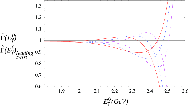
FIG. 3.: Partially integrated Rate (129), normalized to the leading twist result, using the simple model given in (126). The solid, short-dashed and long-dashed lines correspond to $\bar{\Lambda}=570$ MeV, 470 MeV and 370 MeV, respectively. The lines which rise at the endpoint correspond to $\rho_{2}=(500\ {\rm MeV})^{3}$, while those that go down correspond to $\rho_{2}=-(500\ {\rm MeV})^{3}$. The values of $\lambda_{1}$ has been chosen to reproduce the second moment of the leading order structure function, $\lambda_{1}=-0.53\ \bar{\Lambda}^{2}$.

VI Conclusions

It has been known for some time that in inclusive heavy hadron decays the naive short distance expansion must be replaced by a twist expansion if the phase space is restricted to a region of large energy, low invariant mass final hadronic states. The leading term, parametrized by the the light-cone distribution function of the heavy quark in the hadron, is well investigated by now, but subleading terms of this expansion have not been previous studied. In the present paper we have identified the non-local operators appearing at subleading order in the twist expansion. The tree level matching to these operators has been computed for a general bottom hadron decay and the matrix elements of the subleading operators have been parametrized for $B$ meson decay.

We found that for any inclusive $B$ meson decay four independent subleading distribution functions are needed. We worked out the case for $\bar{B}\to X_{s}\gamma$ in detail. Using a simple model for the leading and the subleading distribution functions we studied the effects of the subleading terms on the photon energy spectrum. We found that they had the expected behavior: in the region where the local OPE is appropriate, these corrections were negligible, whereas in the region where the twist expansion was appropriate, they were of order 10-20%, depending on the parameters of the model.

Since the leading distribution function is not known, much less to 10-20% accuracy, these results are of limited utility for $\bar{B}\rightarrow X_{s}\gamma$ decays (although they do indicate the region where the twist expansion breaks down). However, there are certain relations between the charged lepton energy spectrum in $\bar{B}\rightarrow X_{u}\ell\bar{\nu}$ and the photon spectrum in $\bar{B}\rightarrow X_{s}\gamma$ for which the leading distribution function drops out[4, 6]. In this case, even a model of the subleading distribution functions will provide a useful estimate of the theoretical uncertainty in these relations, and the resulting extraction of $|V_{ub}|$. This investigation is in progress [9].

REFERENCES

- [1] M. A. Shifman and M. B. Voloshin, Sov. J. Nucl. Phys. 41, 120 (1985); J. Chay, H. Georgi and B. Grinstein, Phys. Lett. B247, 399 (1990); I. I. Bigi, M. Shifman, N. G. Uraltsev and A. Vainshtein, Phys. Rev. Lett. 71, 496 (1993).
- [2] I. I. Bigi, M. A. Shifman, N. G. Uraltsev and A. I. Vainshtein, Int. J. Mod. Phys. A9, 2467 (1994); M. Neubert, Phys. Rev. D49, 4623 (1994).
- [3] A. F. Falk, Z. Ligeti and M. B. Wise, Phys. Lett. B406, 225 (1997); A. F. Falk, Z. Ligeti, and M. B. Wise, Phys. Lett. B406 (1997) 225; R. D. Dikeman and N. G. Uraltsev, Nucl. Phys. B509, 378 (1998); [hep-ph/9703437] I. Bigi, R. D. Dikeman and N. Uraltsev, Eur. Phys. J. C4, 453 (1998).
- [4] T. Mannel and M. Neubert, Phys. Rev. D 50, 2037 (1994) [hep-ph/9402288].
- [5] C. W. Bauer, Z. Ligeti and M. Luke, Phys. Lett. B479, 395 (2000).
- [6] G. P. Korchemsky and G. Sterman, Phys. Lett. B340, 96 (1994); R. Akhoury and I. Z. Rothstein, Phys. Rev. D 54, 2349 (1996); A. K. Leibovich and I. Z. Rothstein, Phys. Rev. D 61, 074006 (2000); A. K. Leibovich, I. Low and I. Z. Rothstein, Phys. Rev. D 61, 053006 (2000), Phys. Lett. B486, 86 (2000).
- [7] R. K. Ellis, W. Furmanski and R. Petronzio, Nucl. Phys. B212, 29 (1983).
- [8] C. W. Bauer, S. Fleming and M. Luke, Phys. Rev. D 63, 014006 (2001); C. W. Bauer, S. Fleming, D. Pirjol and I. W. Stewart, hep-ph/0011336.
- [9] C. W. Bauer, M. Luke and T. Mannel, in progress.
- [10] T. Mannel, Phys. Rev. D 50, 428 (1994).
- [11] M. Gremm and A. Kapustin, Phys. Rev. D 55, 6924 (1997).
- [12] C. Bauer, Phys. Rev. D 57, 5611 (1998); Erratum-ibid. D 60, 099907 (1999).