General analysis of time evolution of decay spectrum in $B^{0}\rightarrow\pi^{+}\pi^{-}\ell^{+}\ell^{-}$

Using the general, model independent form of effective Hamiltonian, the decay spectrum of $B^{0}\rightarrow\pi^{+}\pi^{-}\ell^{+}\ell^{-}$ decay is studied. The sensitivity of experimentally measurable asymmetries to the new Wilson coefficients and time is studied. It is observed that different asymmetries are sensitive to the new Wilson coefficients and they can serve as an efficient tool for establishing new physics beyond SM.

PACS number(s): 13.20.He, 12.60.–i

1 Introduction

CP violation has been observed in the neutral kaon systems [1, 2]. Great effort is devoted to the study of possible signals of CP violation in $B$ system, which will provide invaluable information about the origin of CP violation and is one of the most promising research area having the potential of establishing new physics beyond the standard model (SM). Started operating, two $B$–factories BaBar and Belle open an excited era for a comprehensive study of $B$ meson physics and especially its rare decays. The main physics program of these factories constitutes a detailed study of CP violation in $B_{d}$ meson and precise measurement of rare flavor–changing neutral current (FCNC) processes. Furthermore, the ultimate goal of these studies is to look for the inconsistencies within the SM (see for example [3]), in particular, to find indications for indications for new physics in the flavor and CP violating sectors. The factories mentioned above have both already signaled the first evidences about the CP violation in neutral $B$ meson decays [4].

One efficient way for detecting CP violation in the neutral $B$ meson decays is the well known Dalitz plot asymmetry [5]. The main advantage of the Dalitz plot asymmetries from the partial rate asymmetries is that they might be present even when partial rate asymmetries vanish. It should be noted that such CP–violating asymmetries in the angular variable $\varphi$ ($\varphi$ is the angle between the $\ell^{+}\ell^{-}$ and $\pi^{+}\pi^{-}$ planes) in the $K\rightarrow\pi^{+}\pi^{-}\ell^{+}\ell^{-}$ decay was measured [2]. In a recent report, NA48 Collaboration [6] confirms large CP–violating effect in the $K\rightarrow\pi^{+}\pi^{-}\ell^{+}\ell^{-}$ decay. Time evolution of the decay spectrum in $K^{0}~{}(\bar{K}^{0}\rightarrow\pi^{+}\pi^{-}\ell^{+}\ell^{-})$ was investigated in framework of the SM in [7].

In this connection several interesting questions come into mind immediately: how does the angular variable asymmetry ${\cal A}_{\varphi}$ evolve with time for the neutral $B$ meson decay? How do new physics effects change the Dalitz plot asymmetry? Can we measure this asymmetry in $B$–factories? This paper is devoted to answering these questions by analyzing the time dependence of the decays $B^{0},~{}\bar{B}^{0}\rightarrow\pi^{+}\pi^{-}\ell^{+}\ell^{-}$ in detail. It should be noted that the $B\rightarrow\pi^{+}\pi^{-}\ell^{+}\ell^{-}$ decay in SM and beyond were studied in [8] and [9], respectively.

The paper is organized as follows. In section 2 we present the general expression of the Dalitz plot asymmetries for the $B^{0}~{}(\bar{B}^{0}\rightarrow\pi^{+}\pi^{-}\ell^{+}\ell^{-})$ decays using the most general, model independent form of the effective Hamiltonian. In section 3 we study the sensitivity of the Dalitz plot asymmetries on the new Wilson coefficients.

2 Time evolution of the decay spectrum of $B^{0}\rightarrow\pi^{+}\pi^{-}\ell^{+}\ell^{-}$

The matrix element for the $B\rightarrow\rho(\rightarrow\pi^{+}\pi^{-})\ell^{+}\ell^{-}$ decay is described by the $b\rightarrow d\ell^{+}\ell^{-}$ transition at quark level. Following [9]–[13], the effective Hamiltonian of the $b\rightarrow d\ell^{+}\ell^{-}$ transition can be written as the sum of the SM and new physics contribution, in a general model independent way in the following form

$${\cal H}_{eff} = \frac{G\alpha}{\sqrt{2}\pi}V_{td}V_{tb}^{\ast}\Bigg{\{}C_{SL}\,\bar{d}i\sigma_{\mu\nu}\frac{q^{\nu}}{q^{2}}\,L\,b\,\bar{\ell}\gamma^{\mu}\ell+C_{BR}\,\bar{d}i\sigma_{\mu\nu}\frac{q^{\nu}}{q^{2}}\,R\,b\,\bar{\ell}\gamma^{\mu}\ell$$

$$+C_{LL}^{tot}\,\bar{d}_{L}\gamma_{\mu}b_{L}\,\bar{\ell}_{L}\gamma^{\mu}\ell_{L}+C_{LR}^{tot}\,\bar{d}_{L}\gamma_{\mu}b_{L}\,\bar{\ell}_{R}\gamma^{\mu}\ell_{R}+C_{RL}\,\bar{d}_{R}\gamma_{\mu}b_{R}\,\bar{\ell}_{L}\gamma^{\mu}\ell_{L}$$

$$+C_{RR}\,\bar{d}_{R}\gamma_{\mu}b_{R}\,\bar{\ell}_{R}\gamma^{\mu}\ell_{R}+C_{LRLR}\,\bar{d}_{L}b_{R}\,\bar{\ell}_{L}\ell_{R}+C_{RLLR}\,\bar{d}_{R}b_{L}\,\bar{\ell}_{L}\ell_{R}$$

$$+C_{LRRL}\,\bar{d}_{L}b_{R}\,\bar{\ell}_{R}\ell_{L}+C_{RLRL}\,\bar{d}_{R}b_{L}\,\bar{\ell}_{R}\ell_{L}+C_{T}\,\bar{d}\sigma_{\mu\nu}b\,\bar{\ell}\sigma^{\mu\nu}\ell$$

$$+iC_{TE}\,\epsilon^{\mu\nu\alpha\beta}\bar{d}\sigma_{\mu\nu}b\,\bar{\ell}\sigma_{\alpha\beta}\ell\Bigg{\}}~{},$$

where the chiral projection operators $L$ and $R$ in (2) are defined as

$$L=\frac{1-\gamma_{5}}{2}~{},~{}~{}~{}~{}~{}~{}R=\frac{1+\gamma_{5}}{2}~{},$$

and $C_{X}$ are the coefficients of the four–Fermi interactions. Here $q=p_{+}+p_{-}$ and $p_{+}$ and $p_{-}$ are the four momenta of $\ell^{+}$ and $\ell^{-}$, respectively. The first two of these coefficients, $C_{SL}$ and $C_{BR}$, are the nonlocal Fermi interactions which correspond to $-2m_{s}C_{7}^{eff}$ and $-2m_{b}C_{7}^{eff}$ in the SM, respectively. The next four terms with coefficients $C_{LL}$, $C_{LR}$, $C_{RL}$ and $C_{RR}$ describe the vector type interactions. Two of these vector interactions containing $C_{LL}^{tot}$ and $C_{LR}^{tot}$ do already exist in the SM in combinations of the form $(C_{9}^{eff}-C_{10})$ and $(C_{9}^{eff}+C_{10})$. Therefore, $C_{LL}^{tot}$ and $C_{LR}^{tot}$ describe the sum of the contributions from SM and the new physics and they are defined as

$$C_{LL}^{tot} = C_{9}^{eff}-C_{10}+C_{LL}~{},$$

$$C_{LR}^{tot} = C_{9}^{eff}+C_{10}+C_{LR}~{}.$$ (2)

The terms with coefficients $C_{LRLR}$, $C_{RLLR}$, $C_{LRRL}$ and $C_{RLRL}$ describe the scalar type interactions. The remaining last two terms leaded by the coefficients $C_{T}$ and $C_{TE}$, obviously, describe the tensor type interactions.

The matrix element for the the process $B\rightarrow\pi^{+}\pi^{-}\ell^{+}\ell^{-}$ can be obtained from the matrix element $B\rightarrow\rho\ell^{+}\ell^{-}$, by the subsequent decay of the $\rho$ meson to pion pair whose interaction Hamiltonian is

$${\cal H}=g_{\rho\pi\pi}(Q\varepsilon)~{},$$ (3)

where $\varepsilon^{\mu}$ is the the polarization four vector of the $\rho$ meson, $Q=p_{\pi^{+}}-p_{\pi^{-}}$ and $p_{\pi^{+}}$ and $p_{\pi^{-}}$ are the four momenta of $\pi^{+}$ and $\pi^{-}$, respectively. Hence, in calculating the 4–body decay amplitude for the $B\rightarrow\pi^{+}\pi^{-}\ell^{+}\ell^{-}$ process, the matrix element of the $B\rightarrow\rho\ell^{+}\ell^{-}$ decay is needed. For this purpose it is enough to sandwich the effective Hamiltonian (2) between the initial and final meson states. In other words, the following matrix elements

$$\left<\rho\left|\bar{d}\gamma_{\mu}(1\pm\gamma_{5})b\right|B\right>~{},$$

$$\left<\rho\left|\bar{d}(1\pm\gamma_{5})b\right|B\right>~{},$$

$$\left<\rho\left|\bar{d}\sigma_{\mu\nu}(1\pm\gamma_{5})b\right|B\right>~{},$$

need to be calculated in order to calculate the decay amplitude for the $B\rightarrow\rho\ell^{+}\ell^{-}$ process. These matrix elements can be written in terms of the form factors as

$$\left<\rho(P,\varepsilon)\left|\bar{d}\gamma_{\mu}(1\pm\gamma_{5})b\right|B(p_{B})\right>=$$

$$-\epsilon_{\mu\nu\lambda\sigma}\varepsilon^{\ast\nu}P^{\lambda}q^{\sigma}\frac{2V(q^{2})}{m_{B}+m_{\rho}}\pm i\varepsilon_{\mu}^{\ast}(m_{B}+m_{\rho})A_{1}(q^{2})$$

$$\mp i(p_{B}+P)_{\mu}(\varepsilon^{\ast}q)\frac{A_{2}(q^{2})}{m_{B}+m_{\rho}}\mp iq_{\mu}\frac{2m_{\rho}}{q^{2}}(\varepsilon^{\ast}q)\left[A_{3}(q^{2})-A_{0}(q^{2})\right]~{}.$$

Multiplying both sides of Eq. (2) with $q_{\mu}$ and using equation of motion, we get

$$\left<\rho(P,\varepsilon)\left|\bar{d}(1\pm\gamma_{5})b\right|B(p_{B})\right>=$$

$$\frac{i}{m_{b}}(\varepsilon^{\ast}q)\Bigg{\{}\mp(m_{B}+m_{\rho})A_{1}(q^{2})\pm(m_{B}^{2}-P^{2})\frac{A_{2}(q^{2})}{m_{B}+m_{\rho}}\pm 2m_{\rho}\Big{[}A_{3}(q^{2})-A_{0}(q^{2})\Big{]}\Bigg{\}}~{}.$$

The remaining matrix element is defined as

$$\left<\rho(P,\varepsilon)\left|\bar{d}\sigma_{\mu\nu}b\right|B(p_{B})\right>=$$

$$i\epsilon_{\mu\nu\lambda\sigma}\Bigg{\{}-2T_{1}(q^{2}){\varepsilon^{\ast}}^{\lambda}(p_{B}+P)^{\sigma}+\frac{2}{q^{2}}(m_{B}^{2}-P^{2})\Big{[}T_{1}(q^{2})-T_{2}(q^{2})\Big{]}{\varepsilon^{\ast}}^{\lambda}q^{\sigma}$$

$$-\frac{4}{q^{2}}\Bigg{[}T_{1}(q^{2})-T_{2}(q^{2})-\frac{q^{2}}{m_{B}^{2}-P^{2}}T_{3}(q^{2})\Bigg{]}(\varepsilon^{\ast}q)P^{\lambda}q^{\sigma}\Bigg{\}}~{}.$$

Moreover, the matrix element $\left<\rho(P,\varepsilon)\left|\bar{d}\sigma_{\mu\nu}\gamma_{5}b\right|B(p_{B})\right>$ can be calculated from Eq. (2) using the identity

$$\sigma_{\mu\nu}\gamma_{5}=-\frac{i}{2}\epsilon_{\mu\nu\alpha\beta}\sigma^{\alpha\beta}~{},$$

which yields

$$\left<\rho(P,\varepsilon)\left|\bar{d}\sigma_{\mu\nu}\gamma_{5}b\right|B(p_{B})\right>=$$ (7)

$$2\Bigg{\{}T_{1}(q^{2})\Big{[}\varepsilon^{\ast}_{\mu}(p_{B}+P)_{\nu}-\varepsilon^{\ast}_{\nu}(p_{B}+P)_{\mu}\Big{]}-\frac{1}{q^{2}}(m_{B}^{2}-P^{2})(\varepsilon^{\ast}_{\mu}q_{\nu}-\varepsilon^{\ast}_{\nu}q_{\mu})\Big{[}T_{1}(q^{2})-T_{2}(q^{2})\Big{]}$$

$$+\frac{2}{q^{2}}\Bigg{[}T_{1}(q^{2})-T_{2}(q^{2})-\frac{q^{2}}{m_{B}^{2}-P^{2}}T_{3}(q^{2})\Bigg{]}(\varepsilon^{\ast}q)(P^{\mu}q^{\nu}-P^{\nu}q^{\mu})\Bigg{\}}~{}.$$

Using Eqs. (3–7) for the matrix element $B\rightarrow\pi^{+}\pi^{-}\ell^{+}\ell^{-}$ decay we get

$${\cal M}(B\rightarrow\pi^{+}\pi^{-}\ell^{+}\ell^{-})=\frac{G\alpha}{4\sqrt{2}}\,V_{tb}V_{td}^{\ast}\,\displaystyle\frac{g^{\nu\alpha}-P^{\nu}P^{\alpha}/m_{\rho}^{2}}{P^{2}-m_{\rho}^{2}+im_{\rho}\Gamma}\,g_{\rho\pi\pi}Q_{\alpha}$$ (8)

$$\times\Bigg{\{}\bar{\ell}\gamma^{\mu}(1-\gamma_{5})\ell\,\Big{[}-2{\cal V}_{L_{1}}\epsilon_{\mu\nu\lambda\sigma}P^{\lambda}q^{\sigma}-i{\cal V}_{L_{2}}g_{\mu\nu}+i{\cal V}_{L_{3}}(2P+q)_{\mu}q_{\nu}+i{\cal V}_{L_{4}}q_{\mu}q_{\nu}\Big{]}$$

$$+\bar{\ell}\gamma^{\mu}(1+\gamma_{5})\ell\,\Big{[}-2{\cal V}_{R_{1}}\epsilon_{\mu\nu\lambda\sigma}P^{\lambda}q^{\sigma}-i{\cal V}_{R_{2}}g_{\mu\nu}+i{\cal V}_{R_{3}}(2P+q)_{\mu}q_{\nu}+i{\cal V}_{R_{4}}q_{\mu}q_{\nu}\Big{]}$$

$$+\bar{\ell}(1-\gamma_{5})\ell\,(iS_{L})q_{\nu}+\bar{\ell}(1+\gamma_{5})\ell\,q_{\nu}(iS_{R})$$

$$+4\bar{\ell}\sigma_{\mu\beta}\ell\Big{(}iC_{T}\epsilon^{\mu\beta\lambda\sigma}\Big{)}\Big{[}-2T_{1}g_{\lambda\nu}(2P+q)_{\sigma}+B_{6}g_{\lambda\nu}q_{\sigma}-B_{7}P_{\lambda}q_{\sigma}q_{\nu}\Big{]}$$

$$+16C_{TE}\bar{\ell}\sigma^{\mu\beta}\ell\Big{[}-2T_{1}g_{\mu\nu}(2P+q)_{\beta}+B_{6}g_{\mu\nu}q_{\beta}-B_{7}q_{\nu}P_{\mu}q_{\beta}\Big{]}\Bigg{\}}~{},$$

where ${\cal{V}}_{L_{i}}$ and ${\cal{V}}_{R_{i}}$ are the coefficients of left– and right–handed leptonic currents with vector structure, respectively, $S_{L,R}$ are the coefficients of the leptonic scalar currents and the last two terms correspond to the contribution of the leptonic tensor currents. These new coefficients are functions of the Wilson coefficients and the form factors introduced in defining the hadronic matrix elements above. Their explicit expressions are given by

$${\cal{V}}_{L_{1}} = (C_{LL}^{tot}+C_{RL})\frac{V}{m_{B}+m_{\rho}}-2(C_{BR}+C_{SL})\frac{T_{1}}{q^{2}},$$

$${\cal{V}}_{L_{2}} = (C_{LL}^{tot}-C_{RL})(m_{B}+m_{\rho})A_{1}-2(C_{BR}-C_{SL})\frac{T_{2}}{q^{2}}(m_{B}^{2}-m_{\rho}^{2})~{},$$

$${\cal{V}}_{L_{3}} = \frac{C_{LL}^{tot}-C_{RL}}{m_{B}+m_{\rho}}A_{2}-2(C_{BR}-C_{SL})\frac{1}{q^{2}}\left[T_{2}+\frac{q^{2}}{m_{B}^{2}-m_{\rho}^{2}}T_{3}\right]~{},$$

$${\cal{V}}_{L_{4}} = (C_{LL}^{tot}-C_{RL})\frac{2m_{\rho}}{q^{2}}(A_{3}-A_{0})-2(C_{BR}-C_{SL})\frac{T_{3}}{q^{2}}~{},$$

$${\cal{V}}_{R_{1}} = {\cal{V}}_{L_{1}}(C_{LL}^{tot}\rightarrow C_{LR}^{tot}~{},~{}~{}C_{RL}\rightarrow C_{RR})~{},$$

$${\cal{V}}_{R_{2}} = {\cal{V}}_{L_{2}}(C_{LL}^{tot}\rightarrow C_{LR}^{tot}~{},~{}~{}C_{RL}\rightarrow C_{RR})~{},$$

$${\cal{V}}_{R_{3}} = {\cal{V}}_{L_{3}}(C_{LL}^{tot}\rightarrow C_{LR}^{tot}~{},~{}~{}C_{RL}\rightarrow C_{RR})~{},$$

$${\cal{V}}_{R_{4}} = {\cal{V}}_{L_{4}}(C_{LL}^{tot}\rightarrow C_{LR}^{tot}~{},~{}~{}C_{RL}\rightarrow C_{RR})~{},$$

$${\cal{S}}_{L} = -(C_{LRRL}-C_{RLRL})\,\frac{1}{m_{b}}\,\Bigg{[}(m_{B}+m_{\rho})A_{1}-(m_{B}^{2}-P^{2})\frac{A_{2}}{m_{B}+m_{\rho}}-2m_{\rho}(A_{3}-A_{0})\Bigg{]}~{},$$

$${\cal{S}}_{R} = -(C_{LRLR}-C_{RLLR})\,\frac{1}{m_{b}}\,\Bigg{[}(m_{B}+m_{\rho})A_{1}-(m_{B}^{2}-P^{2})\frac{A_{2}}{m_{B}+m_{\rho}}-2m_{\rho}(A_{3}-A_{0})\Bigg{]}~{},$$

where dependence on $q^{2}$ is implied. To obtain the amplitudes for the $\bar{B}^{0}\rightarrow\pi^{+}\pi^{-}\ell^{+}\ell^{-}$ decay, it is enough to use CPT invariance and make the replacements in Eq. (8)

$${\cal{V}}_{L_{1};R_{1}} \rightarrow -\overline{\cal{V}}_{L_{1};R_{1}}~{},$$

$${\cal{V}}_{L_{i};R_{i}} \rightarrow \overline{\cal{V}}_{L_{i};R_{i}}~{},~{}~{}~{}(i=2,3,4)~{},$$

$${\cal{S}}_{L;R} \rightarrow \overline{\cal{S}}_{R;L}~{},$$ (9)

$$B_{6;7;8} \rightarrow \bar{B}_{6;7;8}~{},$$

$$B_{9;10;11} \rightarrow -\bar{B}_{9;10;11}~{},$$

where the meaning of the bar can be explained as follows: If any arbitrary one of the coefficients ${\cal{V}}_{L_{i};R_{i}}$ is represented in the form

$${\cal{V}}_{L_{i};R_{i}}=\left|{\cal{V}}_{L_{i};R_{i}}\right|e^{i\delta_{L_{i};R_{i}}}e^{i\phi_{L_{i};R_{i}}}~{},$$

where $\delta$ and $\phi$ are the strong and the weak phases, respectively, then

$$\overline{\cal{V}}_{L_{i};R_{i}}=\left|{\cal{V}}_{L_{i};R_{i}}\right|e^{i\delta_{L_{i};R_{i}}}e^{-i\phi_{L_{i};R_{i}}}~{}.$$

The starting point in analysis of the time evolution spectrum of the $B^{0}(\bar{B}^{0})\rightarrow\pi^{+}\pi^{-}\ell^{+}\ell^{-}$ decay is Eq. (8). The time evolution of the $B$ mesons is given by

$$\left|B^{0}(t)\right> = g_{+}(t)\left|B^{0}\right>+\frac{1}{\xi}g_{-}(t)\left|\bar{B}^{0}\right>~{},$$

$$\left|\bar{B}^{0}(t)\right> = g_{+}(t)\left|\bar{B}^{0}\right>+\xi g_{-}(t)\left|B^{0}\right>~{},$$

with

$$g_{\pm}=exp\left[-\left(\frac{\Gamma_{B}}{2}-im_{B}\right)t\right]\left\{\cos\left(\frac{\Delta m}{2}t\right)~{};~{}\sin\left(\frac{\Delta m}{2}t\right)\right\}~{},$$

and $\xi=p/q$. Here $m_{B}(\Gamma_{B})$ and $\Delta m_{B}(\Delta\Gamma_{B})$ are the average and the difference of the masses (widths) of the two mass eigenstates $B_{H}$ and $B_{L}$, respectively.

The matrix element of the time dependent $B^{0}(t)\rightarrow\pi^{+}\pi^{-}\ell^{+}\ell^{-}$ decay can be obtained from Eq. (8) by making the following replacements.

$${\cal{V}}_{L_{1};R_{1}}\rightarrow{\cal{V}}_{L_{1};R_{1}}(t) = g_{+}(t)\,{\cal{V}}_{L_{1};R_{1}}-\frac{1}{\xi}\,g_{-}(t)\,\overline{\cal{V}}_{L_{1};R_{1}}~{},$$

$${\cal{V}}_{L_{i};R_{i}}\rightarrow{\cal{V}}_{L_{i};R_{i}}(t) = g_{+}(t)\,{\cal{V}}_{L_{i};R_{i}}+\frac{1}{\xi}\,g_{-}(t)\,\overline{\cal{V}}_{L_{i};R_{i}}~{},~{}~{}~{}(i=2,3,4)~{},$$

$${\cal{S}}_{L;R}\rightarrow{\cal{S}}_{L;R}(t) = g_{+}(t)\,{\cal{S}}_{L;R}+\frac{1}{\xi}\,g_{-}(t)\,\overline{\cal{S}}_{R;L}~{},$$ (10)

$$B_{6;7;8}\rightarrow B_{6;7;8}(t) = g_{+}(t)\,B_{6;7;8}+\frac{1}{\xi}\,g_{-}(t)\,\bar{B}_{6;7;8}~{},$$

$$B_{9;10;11}\rightarrow B_{9;10;11}(t) = g_{+}(t)\,B_{9;10;11}-\frac{1}{\xi}\,g_{-}(t)\,\bar{B}_{9;10;11}~{}.$$

Similarly the matrix element for the $\bar{B}^{0}(t)\rightarrow\pi^{+}\pi^{-}\ell^{+}\ell^{-}$ decay can be derived from the respective matrix element ${\cal M}(\bar{B}^{0}\rightarrow\pi^{+}\pi^{-}\ell^{+}\ell^{-})$ with the help of the replacements

$$\overline{\cal{V}}_{L_{1};R_{1}}\rightarrow\overline{\cal{V}}_{L_{1};R_{1}}(t) = g_{+}(t)\,\overline{\cal{V}}_{L_{1};R_{1}}-\xi\,g_{-}(t)\,{\cal{V}}_{L_{1};R_{1}}~{},$$

$$\overline{\cal{V}}_{L_{i};R_{i}}\rightarrow\overline{\cal{V}}_{L_{i};R_{i}}(t) = g_{+}(t)\,\overline{\cal{V}}_{L_{i};R_{i}}+\xi\,g_{-}(t)\,{\cal{V}}_{L_{i};R_{i}}~{},~{}~{}~{}(i=2,3,4)~{},$$

$$\overline{\cal{S}}_{L;R}\rightarrow\overline{\cal{S}}_{L;R}(t) = g_{+}(t)\,\overline{\cal{S}}_{L;R}+\xi\,g_{-}(t)\,{\cal{S}}_{R;L}~{},$$ (11)

$$\bar{B}_{6;7;8}\rightarrow\bar{B}_{6;7;8}(t) = g_{+}(t)\,\bar{B}_{6;7;8}+\xi\,g_{-}(t)\,B_{6;7;8}~{},$$

$$\bar{B}_{9;10;11}\rightarrow\bar{B}_{9;10;11}(t) = g_{+}(t)\,\bar{B}_{9;10;11}-\xi\,g_{-}(t)\,B_{9;10;11}~{}.$$

Using the formalism for the $K_{\ell_{4}}$ decay [14], from the matrix element (8) one can obtain the $B^{0}\rightarrow\pi^{+}\pi^{-}\ell^{+}\ell^{-}$ decay rate in terms of the following five variables: invariant mass $s_{M}=P^{2}=(p_{\pi^{+}}+p_{\pi^{-}})^{2}$ of $\pi^{+}\pi^{-}$ pair, invariant mass $s_{\ell}=q^{2}=(p_{+}+p_{-})^{2}$ of $\ell^{+}\ell^{-}$ pair; the angle $\theta$ between $\vec{p}_{\pi^{+}}$ and $\vec{p}_{+}+\vec{p}_{-}$, measured with respect to the center of mass of $\pi^{+}\pi^{-}$ pair; the angle $\theta_{\ell}$ between $\vec{p}_{+}$ and $\vec{p}_{\pi^{+}}+\vec{p}_{\pi^{-}}$ , measured with respect to the center of mass of $\ell^{+}\ell^{-}$ pair and $\varphi$ is the angle between the normals to the $\pi^{+}\pi^{-}$ and $\ell^{+}\ell^{-}$ planes. The final four–body phase volume in terms of the above–mentioned five variables can be written as

$$dX_{PS}=\frac{1}{2(4\pi)^{6}m_{B}^{2}}X\beta\beta_{\ell}\,ds_{M}\,ds_{\ell}\,d(\cos\theta)\,d(\cos\theta_{\ell})\,d\varphi~{},$$ (12)

where

$$X = \left[\left(Pq\right)^{2}-s_{M}s_{L}\right]^{1/2}~{},$$

$$\beta = \frac{1}{s_{M}}\,\lambda^{1/2}(s_{M},m_{\pi}^{2},m_{\pi}^{2})~{},$$

$$\beta_{\ell} = \frac{1}{s_{\ell}}\,\lambda^{1/2}(s_{\ell},m_{\ell}^{2},m_{\ell}^{2})~{}.$$

The bounds of the integration variables are

$$4m_{\pi}^{2}\!\!\! \leq \!\!\!s_{M}\leq m_{B}^{2}~{},$$

$$4m_{\ell}^{2}\!\!\! \leq \!\!\!s_{\ell}\leq\left(m_{B}-\sqrt{s_{M}}\right)^{2}~{},$$

$$0\!\!\! \leq \!\!\!\theta,\theta_{\ell}\leq\pi~{},$$

$$0\!\!\! \leq \!\!\!\varphi\leq 2\pi~{}.$$

Different scalar quantities appearing in expression of the $\left|{\cal M}\right|^{2}$ can be expressed in terms of the above–mentioned five variables as

$$Pq = \frac{1}{2}(m_{B}^{2}-s_{M}-s_{\ell})~{},$$

$$QN = \beta\beta_{\ell}\left(Pq\,\cos\theta\,\cos\theta_{\ell}-\sqrt{s_{M}s_{\ell}}\,\sin\theta\,\sin\theta_{\ell}\,\cos\varphi\right)~{},$$

$$p_{B}p_{\pm} = \frac{1}{2}\left(s_{M}+Pq\pm X\,\beta\,\cos\theta\right)~{},$$

$$qN = 0~{},$$

$$Qq = X\,\beta\,\cos\theta~{},$$

$$QP = 0~{},$$

$$NP = X\,\beta_{\ell}\,\cos\theta_{\ell}~{},$$

$$Q^{2} = -s_{M}\beta^{2}~{},$$

$$N^{2} = -s_{\ell}\beta_{\ell}^{2}~{},$$

$$\epsilon_{\mu\nu\lambda\sigma}Q^{\mu}P^{\nu}N^{\lambda}q^{\sigma} = -\sqrt{s_{M}s_{\ell}}\,X\,\beta\,\beta_{\ell}\,\sin\theta\,\sin\theta_{\ell}\,\sin\varphi~{},$$

where

$$N=p_{+}-p_{-}~{}.$$

The differential decay rate for the $B^{0}(t)\rightarrow\pi^{+}\pi^{-}\ell^{+}\ell^{-}$ is (in the expression below leptons are taken to be massless. However in calculation of the decay spectrum for $B^{0}(t)\rightarrow\pi^{+}\pi^{-}\tau^{+}\tau^{-}$, the $\tau$ lepton mass is taken into account. But this expression is quite lengthy and for this reason we do not present it in the text)

$$d\Gamma = \left|\frac{G\alpha}{4\sqrt{2}\pi}V_{tb}V_{td}^{\ast}\right|^{2}\,\frac{g_{\rho\pi\pi}^{2}}{\left(s_{M}-m_{\rho}^{2}\right)^{2}+\Gamma^{2}_{\rho}m_{\rho}^{2}}\,\frac{1}{2^{14}\pi^{6}m_{B}^{3}}\,X\,\beta$$ (13)

$$\times ds_{M}\,ds_{\ell}\,d(\cos\theta)\,d(\cos\theta_{\ell})\,d\varphi~{}{\cal I}~{},$$

where

$${\cal I}={\cal I}_{1}\,\cos^{2}\!\theta\,\cos^{2}\!\theta_{\ell}+{\cal I}_{2}\,\cos^{2}\!\theta\,\cos\theta_{\ell}+{\cal I}_{3}\,\cos^{2}\!\theta+{\cal I}_{4}\,\sin^{2}\!\theta\,\sin^{2}\!\theta_{\ell}\,\sin(2\varphi)$$

$$+{\cal I}_{5}\,\sin(2\theta)\,\sin(2\theta_{\ell})\,\cos\varphi+{\cal I}_{6}\,\sin(2\theta)\,\sin(2\theta_{\ell})\,\sin\varphi+{\cal I}_{7}\,\sin(2\theta)\,\sin\theta_{\ell}\,\sin\varphi$$

$$+{\cal I}_{8}\,\sin(2\theta)\,\sin\theta_{\ell}\,\cos\varphi+{\cal I}_{9}\,\cos^{2}\!\theta_{\ell}+{\cal I}_{10}\,\cos\theta_{\ell}+{\cal I}_{11}\,\sin^{2}\!\theta\,\sin^{2}\!\theta_{\ell}\,\cos^{2}\!\varphi+{\cal I}_{12}~{},$$

and

$${\cal I}_{1} = \beta^{2}\Big{\{}\lambda^{2}\Big{[}\left|{\cal V}_{L_{1}}\right|^{2}-\left|{\cal V}_{L_{3}}\right|^{2}+\left|{\cal V}_{R_{1}}\right|^{2}-\left|{\cal V}_{R_{3}}\right|^{2}\Big{]}-2\lambda(Pq)\Big{[}2\,\mbox{\rm Re}\left({\cal V}_{L_{2}}{\cal V}_{L_{3}}^{\ast}\right)$$

$$+ 2\,\mbox{\rm Re}\left({\cal V}_{R_{2}}{\cal V}_{R_{3}}^{\ast}\right)\Big{]}-4\left(Pq\right)^{2}\Big{[}\lambda\left(\left|{\cal V}_{L_{1}}\right|^{2}+\left|{\cal V}_{R_{1}}\right|^{2}\right)+\left|{\cal V}_{L_{2}}\right|^{2}+\left|{\cal V}_{R_{2}}\right|^{2}\Big{]}\Big{\}}~{},$$

$${\cal I}_{2} = 2\beta^{2}\sqrt{\lambda}\Big{[}\lambda-4\left(Pq\right)^{2}\Big{]}\Big{[}-\mbox{\rm Re}\left({\cal V}_{L_{1}}{\cal V}_{L_{2}}^{\ast}\right)+\mbox{\rm Re}\left({\cal V}_{R_{1}}{\cal V}_{R_{2}}^{\ast}\right)\Big{]}~{},$$

$${\cal I}_{3} = \beta^{2}\lambda\Big{\{}\lambda\left(\left|{\cal V}_{L_{3}}\right|^{2}+\left|{\cal V}_{R_{3}}\right|^{2}\right)+\left|{\cal V}_{R_{2}}\right|^{2}-4\left(Pq\right)\Big{[}\mbox{\rm Re}\left({\cal V}_{L_{2}}{\cal V}_{L_{3}}^{\ast}\right)+\mbox{\rm Re}\left({\cal V}_{R_{2}}{\cal V}_{R_{3}}^{\ast}\right)\Big{]}\Big{\}}~{},$$

$${\cal I}_{4} = 4\beta^{2}\sqrt{\lambda}\Big{[}\mbox{\rm Im}\left({\cal V}_{L_{2}}{\cal V}_{L_{1}}^{\ast}\right)+\mbox{\rm Im}\left({\cal V}_{R_{2}}{\cal V}_{L_{1}}^{\ast}\right)\Big{]}~{},$$

$${\cal I}_{5} = -\beta^{2}\sqrt{s_{M}s_{\ell}}\,\Big{\{}\lambda\Big{[}\mbox{\rm Re}\left({\cal V}_{L_{2}}{\cal V}_{L_{3}}^{\ast}\right)+\mbox{\rm Re}\left({\cal V}_{R_{2}}{\cal V}_{R_{3}}^{\ast}\right)\Big{]}-2\left(Pq\right)\left(\left|{\cal V}_{L_{2}}\right|^{2}+\left|{\cal V}_{R_{2}}\right|^{2}\right)\Big{\}}~{},$$

$${\cal I}_{6} = \beta^{2}\sqrt{\lambda}\,\Big{\{}\lambda\Big{[}\mbox{\rm Im}\left({\cal V}_{L_{3}}{\cal V}_{L_{1}}^{\ast}\right)+\mbox{\rm Im}\left({\cal V}_{R_{3}}{\cal V}_{R_{1}}^{\ast}\right)\Big{]}+2\left(Pq\right)\Big{[}\mbox{\rm Im}\left({\cal V}_{L_{1}}{\cal V}_{L_{2}}^{\ast}\right)$$

$$+ \mbox{\rm Im}\left({\cal V}_{R_{1}}{\cal V}_{R_{2}}^{\ast}\right)\Big{]}\Big{\}}~{},$$

$${\cal I}_{7} = 2\beta^{2}\lambda\,\sqrt{s_{M}s_{\ell}}\,\Big{[}\mbox{\rm Im}\left({\cal V}_{L_{3}}{\cal V}_{L_{2}}^{\ast}\right)-\mbox{\rm Im}\left({\cal V}_{R_{3}}{\cal V}_{R_{2}}^{\ast}\right)\Big{]}~{},$$

$${\cal I}_{8} = 2\beta^{2}\sqrt{\lambda s_{M}s_{\ell}}\,\Big{\{}\lambda\Big{[}\mbox{\rm Re}\left({\cal V}_{L_{1}}{\cal V}_{L_{3}}^{\ast}\right)-\mbox{\rm Re}\left({\cal V}_{R_{1}}{\cal V}_{R_{3}}^{\ast}\right)\Big{]}+2\left(Pq\right)\Big{[}-\mbox{\rm Re}\left({\cal V}_{L_{1}}{\cal V}_{L_{2}}^{\ast}\right)$$

$$+ \mbox{\rm Re}\left({\cal V}_{R_{1}}{\cal V}_{R_{2}}^{\ast}\right)\Big{]}\Big{\}}~{},$$

$${\cal I}_{9} = 4\beta^{2}s_{\ell}s_{M}\lambda\,\Big{[}\left|{\cal V}_{L_{1}}\right|^{2}+\left|{\cal V}_{R_{1}}\right|^{2}\Big{]}~{},$$

$${\cal I}_{10} = 8\beta^{2}\sqrt{\lambda}\,\Big{[}-\mbox{\rm Re}\left({\cal V}_{L_{1}}{\cal V}_{L_{2}}^{\ast}\right)+\mbox{\rm Re}\left({\cal V}_{R_{1}}{\cal V}_{R_{2}}^{\ast}\right)\Big{]}~{},$$

$${\cal I}_{11} = 4\beta^{2}s_{\ell}s_{M}\,\Big{[}\lambda\left(\left|{\cal V}_{L_{1}}\right|^{2}+\left|{\cal V}_{R_{1}}\right|^{2}\right)-\left|{\cal V}_{L_{2}}\right|^{2}-\left|{\cal V}_{R_{2}}\right|^{2}\Big{]}~{},$$

$${\cal I}_{12} = 4\beta^{2}s_{\ell}s_{M}\,\Big{[}\left|{\cal V}_{L_{2}}\right|^{2}+\left|{\cal V}_{R_{2}}\right|^{2}\Big{]}~{}.$$

Taking the narrow resonance limit of $\rho$ meson, i.e., using the equations

$$\Gamma=\frac{g_{\rho\pi\pi}^{2}m_{\rho}}{48\pi}\left(1-\frac{4m_{\pi}^{2}}{m_{\rho}^{2}}\right)^{3/2}~{},~{}~{}~{}\mbox{\rm and},$$

$$\lim_{\Gamma\rightarrow 0}\,\frac{\Gamma m_{\rho}}{\left(s_{M}-m_{\rho}^{2}\right)^{2}+m_{\rho}^{2}\Gamma^{2}}=\pi\delta\left(s_{M}-m_{\rho}^{2}\right)~{},$$

we perform integration over $s_{M}$ easily in Eq. (2). After integrating over $s_{M}$, $s_{\ell}$ and $\theta$, we get for the angular distribution of the $B^{0}(t)\rightarrow\pi^{+}\pi^{-}\ell^{+}\ell^{-}$ decay

$$\frac{d\Gamma}{d(cos\theta_{\ell})\,d\varphi}=\left|\frac{G\alpha}{4\sqrt{2}\pi}\,V_{tb}V_{td}^{\ast}\right|^{2}\,\frac{1}{2^{14}\pi^{6}m_{B}^{3}}\,\frac{48\pi^{2}}{m_{\rho}^{2}\left(1-4m_{\pi}^{2}/m_{\rho}^{2}\right)^{1/2}}$$ (15)

$$\times\Bigg{\{}\left(\frac{2}{3}{\cal I}_{1}^{\prime}+2{\cal I}_{9}^{\prime}\right)\cos^{2}\!\theta_{\ell}+\left(\frac{2}{3}{\cal I}_{2}^{\prime}+2{\cal I}_{10}^{\prime}\right)\cos\theta_{\ell}+\frac{4}{3}{\cal I}_{4}^{\prime}\sin^{2}\!\theta_{\ell}\,\sin(2\varphi)$$

$$+\frac{2}{3}{\cal I}_{11}^{\prime}\sin^{2}\!\theta_{\ell}\Big{[}1+\cos(2\varphi)\Big{]}+\left(\frac{2}{3}{\cal I}_{3}^{\prime}+2{\cal I}_{12}^{\prime}\right)\Bigg{\}}~{},$$

where we have introduced the notation ${\cal I}_{i}^{\prime}\equiv\int X{\cal I}_{i}\,ds_{\ell}$. CP violation manifests itself in the coefficients $\sim{\cal I}_{4}^{\prime}$ and $\sim{\cal I}_{11}^{\prime}$. The dominant CP violation term is contained in the coefficient $(4/3){\cal I}_{4}^{\prime}$. After integrating over $\cos\theta_{\ell}$ we obtain the $\varphi$–distribution

$$\frac{d\Gamma}{d\varphi}\sim\frac{2}{3}\left(\frac{2}{3}{\cal I}_{1}^{\prime}+2{\cal I}_{9}^{\prime}\right)+\frac{16}{9}{\cal I}_{4}^{\prime}\sin(2\varphi)+\frac{8}{9}{\cal I}_{11}^{\prime}\Big{[}1+\cos(2\varphi)\Big{]}+2\left(\frac{2}{3}{\cal I}_{3}^{\prime}+2{\cal I}_{12}^{\prime}\right)~{}.$$

As has already been noted the term $\sim\sin(2\varphi)$ is CP– and T–odd. Hence this term can be isolated by considering the following asymmetry in terms of the differential decay rates of the $B$ meson with respect to $\varphi$

$${\cal A}_{\varphi}(t)=\frac{\displaystyle\left\{\int_{0}^{\pi/2}\,-\,\int_{\pi/2}^{\pi}\,+\int_{\pi}^{3\pi/2}\,-\,\int_{3\pi/2}^{2\pi}\right\}\displaystyle\frac{d\Gamma}{d\varphi}\,d\varphi}{\displaystyle\left\{\int_{0}^{\pi/2}\,+\,\int_{\pi/2}^{\pi}\,+\int_{\pi}^{3\pi/2}\,+\,\int_{3\pi/2}^{2\pi}\right\}\displaystyle\frac{d\Gamma}{d\varphi}\,d\varphi}~{}.$$

The main feature of such CP violating asymmetries is that they can be obtained by considering the sum of the differential decay rates of the $B$ and $\bar{B}$ rather than the difference of these rates, as usual.

Furthermore we study the dependence of the asymmetry between the spectrum integrated rates of $B^{0}(t)\rightarrow\pi^{+}\pi^{-}\ell^{+}\ell^{-}$ and $\bar{B}^{0}(t)\rightarrow\pi^{+}\pi^{-}\ell^{+}\ell^{-}$ decays, on the new Wilson coefficients, which is defined as

$${\cal A}_{1}(t)=\frac{\displaystyle\Gamma(B^{0}(t)\rightarrow\pi^{+}\pi^{-}\ell^{+}\ell^{-})-\Gamma(\bar{B}^{0}(t)\rightarrow\pi^{+}\pi^{-}\ell^{+}\ell^{-})}{\displaystyle\Gamma(B^{0}(t)\rightarrow\pi^{+}\pi^{-}\ell^{+}\ell^{-})+\Gamma(\bar{B}^{0}(t)\rightarrow\pi^{+}\pi^{-}\ell^{+}\ell^{-})}~{}.$$ (16)

It should noted that it is also possible to construct a differential asymmetry that isolates another combination of the terms containing imaginary parts (see for example [15, 16]). Such terms, for example, can be isolated by considering the difference distribution of the same hemisphere and opposite hemisphere events. The corresponding asymmetry can be defined then as follows

$${\cal A}_{2}(t) = \frac{1}{\Gamma}\,\left\{\int_{0}^{\pi}\,-\,\int_{0}^{2\pi}\right\}d\varphi\,\left\{\int_{-1}^{0}\,-\,\int_{0}^{+1}\right\}d(\cos\theta_{\ell})\,\left\{\int_{-1}^{0}\,-\,\int_{0}^{+1}\right\}d(\cos\theta)$$ (17)

$$\times \frac{d\Gamma}{d\varphi\,d(\cos\theta_{\ell})\,d(\cos\theta)}~{}.$$

3 Numerical analysis

In this section we study the dependence of the asymmetries ${\cal A}_{\varphi},~{}{\cal A}_{1}$ and ${\cal A}_{2}$ on new Wilson coefficients and time for the $B^{0}(t)\rightarrow\pi^{+}\pi^{-}\ell^{+}\ell^{-}$ decay. Before presenting the numerical results we want to note that, although the expressions for the asymmetries ${\cal A}_{\varphi},~{}{\cal A}_{1}$ and ${\cal A}_{2}$ are given for the most general case, i.e., each one of new Wilson coefficients might have new strong and weak phases. In our numerical analysis we choose all new Wilson coefficients to be real and they all vary in the region between $-4$ and $+4$.

For the form factors which are needed in the course of performing numerical calculations, we have used the prediction of the light cone QCD sum rules. In our numerical analysis we will use the results of the work [17] (see also [18, 19]) in which the form factors are described by a three–parameter fit where the radiative corrections up to leading twist contribution and SU(3)–breaking effects are taken into account. The $q^{2}$–dependence of the form factors which appear in our analysis could be parametrized as

$$F(s)=\frac{F(0)}{1-a_{F}\,s+b_{F}\,s^{2}}~{},$$

where $s=q^{2}/m_{B}^{2}$ is the dilepton invariant mass in units of $B$ meson mass, and the parameters $F(0)$, $a_{F}$ and $b_{F}$ are listed in Table 1 for each form factor.

$$\begin{array}[]{|l|ccc|}\hline\cr&F(0)&a_{F}&b_{F}\\ \hline\cr A_{0}^{B\rightarrow\rho}&\phantom{-}0.372&1.40&\phantom{-}0.437\\ A_{1}^{B\rightarrow\rho}&\phantom{-}0.261&0.29&-0.415\\ A_{2}^{B\rightarrow\rho}&\phantom{-}0.223&0.93&-0.092\\ V^{B\rightarrow\rho}&\phantom{-}0.338&1.37&\phantom{-}0.315\\ T_{1}^{B\rightarrow\rho}&\phantom{-}0.143&1.41&\phantom{-}0.361\\ T_{2}^{B\rightarrow\rho}&\phantom{-}0.143&0.28&-0.500\\ T_{3}^{B\rightarrow\rho}&\phantom{-}0.101&1.06&-0.076\\ \hline\cr\end{array}$$

Table 1: The form factors for $B\rightarrow\rho\ell^{+}\ell^{-}$ in a three–parameter fit.

As it comes to the values of the Wilson coefficients $C_{7}^{eff}(m_{b})$ and $C_{10}(m_{b})$, whose analytical expressions in the standard model are given in [20, 21], are strictly real as can be read off from Table 2. In the leading logarithmic approximation, at the scale ${\cal O}(\mu=m_{b})$, we have

$$C_{7}^{eff}(m_{b}) = -0.313~{},$$

$$C_{10}^{eff}(m_{b}) = -4.669~{}.$$

$$\begin{array}[]{|c|c|c|c|c|c|c|c|c|c|}\hline\cr C_{1}&C_{2}&C_{3}&C_{4}&C_{5}&C_{6}&C_{7}^{eff}&C_{9}&C_{10}^{eff}&C^{(0)}\\ \hline\cr-0.248&1.107&0.011&-0.026&0.007&-0.031&-0.313&4.344&-4.669&0.362\\ \hline\cr\end{array}$$

Table 2: The numerical values of the Wilson coefficients at $\mu\sim m_{b}$ scale within the SM.

Although individual Wilson coefficients at $\mu\sim m_{b}$ level are all real (see Table 2), the effective Wilson coefficient $C_{9}^{eff}(m_{b},\hat{s})$ has a finite phase, and in next–to–leading order

$$C_{9}^{eff}(m_{b},\hat{s})=C_{9}(m_{b})\left[1+\frac{\alpha_{s}(\mu)}{\pi}\omega(\hat{s})\right]+Y_{SD}(m_{b},\hat{s})+Y_{LD}(m_{B},s)~{},$$ (18)

where $C_{9}(m_{b})=4.344$. Here $\omega\left(\hat{s}\right)$ represents the ${\cal{O}}(\alpha_{s})$ corrections coming from one–gluon exchange in the matrix element of the corresponding operator, whose explicit form can be found in [20]. In (18) $Y_{SD}$ and $Y_{LD}$ represent, respectively, the short– and long–distance contributions of the four–quark operators ${\cal{O}}_{i=1,\cdots,6}$ [20, 21]. Here $Y_{SD}$ can be obtained by a perturbative calculation

$$Y_{SD}\left(m_{b},\hat{s}\right) = g\left(\hat{m}_{c},\hat{s}\right)C^{(0)}-\frac{1}{2}g\left(1,\hat{s}\right)\left[4C_{3}+4C_{4}+3C_{5}+C_{6}\right]$$

$$- \frac{1}{2}g\left(0,\hat{s}\right)\left[C_{3}+3C_{4}\right]+\frac{2}{9}\left[3C_{3}+C_{4}+3C_{5}+C_{6}\right]$$

$$- \lambda_{u}\left[3C_{1}+C_{2}\right]\left[g\left(0,\hat{s}\right)-g\left(\hat{m}_{c},\hat{s}\right)\right]~{},$$

where

$$C^{(0)} = 3C_{1}+C_{2}+3C_{3}+C_{4}+3C_{5}+C_{6}~{},$$

$$\lambda_{u} = \frac{V_{ub}V_{ud}^{\ast}}{V_{tb}V_{td}^{\ast}}~{},$$

and the loop function $g\left(m_{q},s\right)$ stands for the loops of quarks with mass $m_{q}$ at the dilepton invariant mass $s$. This function develops absorptive parts for dilepton energies $s=4m_{q}^{2}$:

$$g\left(\hat{m}_{q},\hat{s}\right)=-\frac{8}{9}\ln\hat{m}_{q}+\frac{8}{27}+\frac{4}{9}y_{q}-\frac{2}{9}\left(2+y_{q}\right)\sqrt{\left|1-y_{q}\right|}$$

$$\times\Bigg{[}\Theta(1-y_{q})\left(\ln\frac{1+\sqrt{1-y_{q}}}{1-\sqrt{1-y_{q}}}-i\pi\right)+\Theta(y_{q}-1)\,2\,\arctan\frac{1}{\sqrt{y_{q}-1}}\Bigg{]},$$

where $\hat{m}_{q}=m_{q}/m_{b}$ and $y_{q}=4\hat{m}_{q}^{2}/\hat{s}$. In addition to these perturbative contributions $\bar{c}c$ loops can excite low–lying charmonium states $\psi(1s),\cdots,\psi(6s)$ whose contributions are represented by $Y_{LD}$ [22]. However in the present work we restrict ourselves to the consideration of short distance contributions only and therefore we find it redundant to display the explicit form of $Y_{LD}$.

Calculations show that the asymmetry ${\cal A}_{\varphi}$ for the $B^{0}(t)\rightarrow\pi^{+}\pi^{-}\mu^{+}\mu^{-}$ decay is sensitive only to tensor type interaction. We observe that, practically, the existence of the new vector or scalar type interactions do not effect the SM results crucially, which is about $13\%$. However when tensor type interactions are taken into consideration this asymmetry is reduced noticeably and $\left({\cal A}_{\varphi}\right)_{max}\sim 2.5\%$. Therefore if in future experiments the results obtained results differ from the SM results, it is an unambiguous indication of the existence of new physics beyond SM.

As one considers the $B^{0}(t)\rightarrow\pi^{+}\pi^{-}\tau^{+}\tau^{-}$ decay, the maximum value of the asymmetry ${\cal A}_{\varphi}$ is about $5\%$. Similarly, as in the $B^{0}(t)\rightarrow\pi^{+}\pi^{-}\mu^{+}\mu^{-}$ decay, ${\cal A}_{\varphi}$ is not sensitive to the new vector and scalar interactions and for the contribution of the tensor interaction is less $1\%$.

We further studied the dependence of the asymmetry ${\cal A}_{1}$ on the new Wilson coefficients and time for both $B^{0}(t)\rightarrow\pi^{+}\pi^{-}\mu^{+}\mu^{-}$ and $B^{0}(t)\rightarrow\pi^{+}\pi^{-}\tau^{+}\tau^{-}$ decays. Our calculations show that the maximal possible value that ${\cal A}_{1}$ asymmetry gets for the $B^{0}(t)\rightarrow\pi^{+}\pi^{-}\mu^{+}\mu^{-}$ decay is about $2\%$ for all type of new interactions. Similar behavior takes place for the $B^{0}(t)\rightarrow\pi^{+}\pi^{-}\tau^{+}\tau^{-}$ case as well, with only one exception. For tensor type interactions which are controlled by the new Wilson coefficients $C_{T}$ and $C_{TE}$, ${\cal A}_{1}$ can arrive at large values about $20\%$ (see Figs. (1) and (2)). So any departure from the SM prediction in future experiments, is an indication of the presence of tensor type interactions.

Finally we have studied the dependence of the ${\cal A}_{2}$ asymmetry on new Wilson coefficients and time for the above mentioned decays. For the $B^{0}(t)\rightarrow\pi^{+}\pi^{-}\mu^{+}\mu^{-}$ decay the maximal value of ${\cal A}_{2}$ is about coefficient $C_{LL}=-4$ causes ${\cal A}_{2}$ to decrease about $50\%$ from the SM prediction, but if $C_{LL}=+4$, practically the value of ${\cal A}_{2}$ seems to coincide with the SM prediction, which also gives us a clue in determining the sign of of the new vector interaction, as can be seen in Fig. (3). As is depicted in Fig. (4), similar situation seems to hold for the new Wilson coefficient $C_{RL}$. Our numerical analysis shows that ${\cal A}_{2}$ is quite insensitive to the existence of scalar interaction and yields almost same results with SM prediction. But an important observation is that the tensor interaction enhances the SM prediction by about $50\%$. Therefore it would be an unambiguous confirmation of the existence of new vector (tensor) interaction, if in future experiments the measured value of ${\cal A}_{2}$ appears to be less (larger) than the SM prediction.

On the other hand for all values of the new Wilson coefficients, the ${\cal A}_{2}$ asymmetry for the $B^{0}(t)\rightarrow\pi^{+}\pi^{-}\tau^{+}\tau^{-}$ case coincides almost with the SM prediction. For this reason ${\cal A}_{2}$ for $B^{0}(t)\rightarrow\pi^{+}\pi^{-}\tau^{+}\tau^{-}$ decay does not seem to provide us with any new information about new physics beyond SM.

As a final remark we should emphasize that similar analysis can be performed for the $\bar{B}^{0}(t)\rightarrow\pi^{+}\pi^{-}\ell^{+}\ell^{-}$ decay as well. For this aim it is enough to use Eqs. (8), (2) and (2).

In conclusion, in this work we have studied the time evolution of the decay spectrum for the $B^{0}(t)\rightarrow\pi^{+}\pi^{-}\ell^{+}\ell^{-}$ decay. The sensitivity of the experimentally measurable asymmetries ${\cal A}_{\varphi}$, ${\cal A}_{1}$ and ${\cal A}_{2}$ to the new Wilson coefficients and time is studied in detail. It is observed that different asymmetries show different dependencies on different new Wilson coefficients for the $B^{0}(t)\rightarrow\pi^{+}\pi^{-}\mu^{+}\mu^{-}$ and $B^{0}(t)\rightarrow\pi^{+}\pi^{-}\tau^{+}\tau^{-}$ channels. Studying different asymmetries for the above–mentioned two channels on new Wilson coefficients can give essential information about new physics and can serve as an efficient tool in determining not only of the magnitude, but also of the sign of new Wilson coefficients.

Figure captions

Fig. (1) The dependence of the asymmetry ${\cal A}_{1}$ on the new Wilson coefficient $C_{T}$ and time for $B^{0}(t)\rightarrow\pi^{+}\pi^{-}\tau^{+}\tau^{-}$ decay, where $\tau_{s}$ is the $B^{0}$ meson life time.

Fig. (2) The same as in Fig. (1), but for the new Wilson coefficient $C_{TE}$.

Fig. (3) The dependence of the asymmetry ${\cal A}_{2}$ on the new Wilson coefficient $C_{LL}$ and time for $B^{0}(t)\rightarrow\pi^{+}\pi^{-}\mu^{+}\mu^{-}$ decay.

Fig. (4) The same as in Fig. (3), but for the new Wilson coefficient $C_{RL}$.

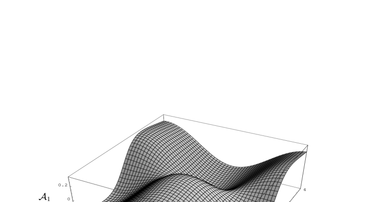
Figure 1:

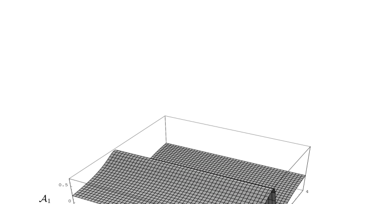
Figure 2:

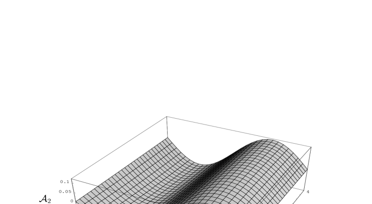
Figure 3:

Figure 4:

References

• [1] J. H. Christenson, J. W. Gronin, V. L. Fitch, R. Turlay, Phys. Rev. Lett. D13 (1964) 138.
• [2] KTeV Collaboration, A. Alavi–Harati at al, Phys. Rev. Lett. 84 (2000) 408.
• [3] Y. Grossman, preprint: hep-ph/0012216 (2000).
• [4] BaBar Collaboration, D. Hitlin, preprint: hep-ex/0011024 (2000);
Belle Collaboration, H. Aihara, preprint: hep-ex/0010008 (2000).
• [5] G. Burdman and J. F. Donoghue, Phys. Rev. D54 (1992) 187.
• [6] NA48 Collaboration, A. Lai at al, Phys. Lett. B496 (2000) 137.
• [7] L. M. Sehgal and J. van Leusen, Phys. Lett. B489 (2000) 300.
• [8] F. Krüger, L. M. Sehgal, N. Sinha and R. Sinha, Phys. Rev. D61 (2000) 114028;
Erratum, ibid D63 (2001) 019901.
• [9] T. M. Aliev and M. Savcı, Phys. Rev. D62 (2000) 114010.
• [10] S. Fukae, C. S. Kim and T. Yoshikawa, Phys. Rev. D61 (2000) 074015.
• [11] S. Fukae, C. S. Kim, T. Morozumi and T. Yoshikawa, Phys. Rev. D59 (1999) 074013.
• [12] T. M. Aliev, C. S. Kim and Y. G. Kim,, Phys. Rev. D62 (2000) 014026.
• [13] T. M. Aliev, D. A. Demir, M. Savcı, Phys. Rev. D62 (2000) 074016.
• [14] A. Pais and S. B. Treiman, Phys. Rev. 168 (1968) 1858.
• [15] G. Kramer and W. F. Palmer, Phys. Lett. B279 (1992) 181.
• [16] R. Sinha, preprint: hep-ph/9608314 (1996).
• [17] P. Ball and V. M. Braun, Phys. Rev. D58(1998) 094016.
• [18] P. Ball, JHEP 9809 (1998) 005.
• [19] T. M. Aliev, A. Özpineci and M. Savcı, Phys. Rev. D55 (1997) 7059.
• [20] M. Misiak, Nucl. Phys. B393 (1993) 23; Erratum, ibid B439 (1995) 461.
• [21] A. J. Buras and M. Münz, Phys. Rev. D52 (1995) 186.
• [22] N. G. Deshpande, J. Trampetic and K. Panose, Phys. Rev. D39 (1989) 1461;
C. S. Lim, T. Morozumi and A. I. Sanda, Phys. Lett. B218 (1989) 343.