Abstract

We calculate the cross sections for the neutral Higgs-boson production at $e^{+}e^{-}$ colliders in the Minimal Supersymmetric Standard Model (MSSM) using the Feynman-diagrammatic approach and the on-shell renormalization scheme. We incorporate the Higgs-boson propagator corrections, evaluated up to two-loop order, into the prediction of the cross sections for the Higgs-boson production mechanism $e^{+}e^{-}\to hZ,hA$. The propagator corrections consist of the full one-loop contribution, including the effects of non-vanishing external momentum, and at the two-loop level of the dominant corrections of ${\cal O}(\alpha\alpha_{s})$ and further sub-dominant contributions. The results are supplemented with the complete set of one-loop vertex and box corrections. The effects of the two-loop propagator corrections are investigated in detail. We briefly discuss also the effect of the box contributions for high $\sqrt{s}$. We compare our results with the case where only the corrections to the effective mixing angle, evaluated within the renormalization-group-improved one-loop Effective Potential approach, are taken into account. We find agreement better than 10% for LEP2 energies and deviations larger than 20% for $\sqrt{s}=500$ GeV.

1 Introduction

The search for the light neutral Higgs boson is a crucial test of Supersymmetry that can be performed with the present and the next generation of accelerators. The prediction of a relatively light Higgs boson is common to all supersymmetric models whose couplings remain in the perturbative regime up to a very high energy scale [1]. Finding the Higgs boson is thus one of the main goals of high-energy physics. Possible indications for a Higgs boson with a mass around $115\,\,\mathrm{GeV}$ have recently been observed in the LEP analysis [2]. As a second step, once a scalar particle has been found, it is necessary to measure the dominant production cross sections as well as the decay widths and branching ratios of the main decay channels to a high accuracy. Such precise measurements of Higgs–gauge-boson and Higgs–Yukawa couplings allow to experimentally investigate the details of the Higgs mechanism. Finally, also the Higgs self-couplings will have to be measured in order to reconstruct the Higgs potential. A future linear $e^{+}e^{-}$ collider with high luminosity [3] can provide a sufficiently clean environment to measure both the Higgs couplings to other particles as well as its self couplings [4] with high precision, allowing to distinguish between a standard and a non-standard Higgs boson. In this paper we concentrate on the production of the neutral Higgs bosons of the Minimal Supersymmetric Standard Model (MSSM) in $e^{+}e^{-}$ annihilations and provide results for the production cross sections for general model parameters, together with a detailed numerical study.

In the MSSM, the mass of the lightest Higgs boson, $M_{h}$, is bounded from above by $M_{h}\;\raisebox{-3.00003pt}{$\stackrel{{\scriptstyle\displaystyle<}}{{\sim}}$}\;135\,\,\mathrm{GeV}$, including radiative corrections up to two-loop order [5, 6, 7, 8, 9, 10, 12, 13, 11]. The most promising channels for the production of the supersymmetric neutral Higgs particles at LEP2 energies and in the first phase of future $e^{+}e^{-}$ colliders are the Higgs-strahlung process [14]

$$e^{+}e^{-}\to Z\,h\,(H),$$ (1)

and the associated production of a scalar and a pseudoscalar Higgs boson

$$e^{+}e^{-}\to A\,h\,(H)~{}.$$ (2)

We compute the MSSM predictions for the cross sections of both channels in the Feynman-diagrammatic (FD) approach using the on-shell renormalization scheme. We take into account the complete set of one-loop contributions, thereby keeping the full dependence on all kinematical variables. The one-loop contributions consist of the corrections to the Higgs- and gauge-boson propagators, where the former contain the dominant electroweak one-loop corrections of ${\cal O}(G_{F}m_{t}^{4})$, and of the contributions to the 3-point and 4-point vertex functions [15, 16, 17, 18, 19]. We combine the complete one-loop result with the dominant two-loop QCD corrections of ${\cal O}(G_{F}\alpha_{s}m_{t}^{4})$ [12, 13] and further sub-dominant corrections. In this way the currently most accurate results for the cross sections are obtained.

Furthermore we show analytically that the Higgs-boson propagator corrections with neglected momentum dependence can be absorbed into the tree-level coupling using the effective mixing angle from the neutral ${\cal CP}$-even Higgs-boson sector. We compare our results for the cross sections with the approximation in which only the corrections to the effective mixing angle, evaluated within the renormalization-group-improved one-loop Effective Potential approach, are taken into account. For most parts of the MSSM parameter space we find agreement better than 10% for the highest LEP energies, while for $\sqrt{s}=500\,\,\mathrm{GeV}$ the difference can reach 25%.

The paper is organized as follows: in section 2 the basic formulae are presented and it is shown analytically how the Higgs-boson-propagator corrections with neglected external momenta are related to the effective mixing angle in the Effective Potential approach (EPA). Section 3 contains the numerical analysis for the production cross sections and the comparison of our full result with the EPA. The conclusions can be found in section 4.

2 Cross sections for Higgs-particle production in $e^{+}e^{-}$ collisions

2.1 Classification of radiative corrections

The two Higgs-field doublets giving rise to electroweak symmetry breaking within the MSSM accommodate five physical Higgs bosons [20]. At the tree-level, two input parameters (besides the parameters of the Standard Model (SM) gauge-sector) are needed to describe the Higgs sector. We choose them to be $\tan\beta$, the ratio of the two vacuum expectation values, and $M_{A}$, the mass of the ${\cal CP}$-odd Higgs boson. The ${\cal CP}$-even neutral mass eigenstates are obtained from the interaction eigenstates by the rotation

$$\left(\begin{array}[]{c}H_{1}\\ H_{2}\end{array}\right)\equiv\left(\begin{array}[]{c}H\\ h\end{array}\right)=\left(\begin{array}[]{cc}\cos\alpha&\sin\alpha\\ -\sin\alpha&\cos\alpha\end{array}\right)\left(\begin{array}[]{c}\phi_{1}^{0}\\ \phi_{2}^{0}\end{array}\right)$$ (3)

with the tree-level mixing angle $\alpha$ related to $\tan\beta$, $M_{A}$ and $M_{Z}$ by

$$\tan 2\alpha=\tan 2\beta\frac{M_{A}^{2}+M_{Z}^{2}}{M_{A}^{2}-M_{Z}^{2}},\quad-\frac{\pi}{2}<\alpha<0.$$ (4)

Two main sources for the production of supersymmetric Higgs particles in $e^{+}e^{-}$ collisions are the Higgs-strahlung process [14]

$$e^{+}e^{-}\to ZH_{i},~{}i=1,2$$ (5)

(using the compact notation of eq. (3)) and the associated production of scalar and pseudoscalar Higgs bosons,

$$e^{+}e^{-}\to AH_{i},~{}i=1,2.$$ (6)

We do not discuss here the possibility of Higgs-particle production by bremsstrahlung off heavy quarks (e.g. $e^{+}e^{-}\to\bar{b}bH_{i}$, which can be significant for large $\tan\beta$ [21]), or by $W^{+}W^{-}$ fusion, which becomes important for center of mass system (CMS) energies of ${\cal O}(500$ GeV) [14].

The set of diagrams taken into account for Higgs-strahlung $e^{+}e^{-}\to hZ$ is schematically shown in Fig. 1, where a) is the tree-level diagram. The shaded blobs summarize the loops with all possible virtual particles, except photons in the $Ze^{+}e^{-}$ vertex corrections. More details can be found in Refs. [16, 18, 19]. An analogous set has been evaluated for the second process, $e^{+}e^{-}\to hA$.

Figure 1: Generic diagrams contributing to the $e^{+}e^{-}\rightarrow Zh$ cross section.

For completeness, in Fig. 1 also contributions are shown (e.g. the $A,G$–$Z$ mixing contributions and the longitudinal parts of the $Z$ and $\gamma$–$Z$ self-energies) that are proportional to the electron mass or vanish completely after contraction with the polarization vector of the $Z$ boson. The different types of corrections can be summarized as follows:

• Corrections to the $e$, $Z$, $\gamma$ and $\gamma$–$Z$ self-energies on the internal and external lines and to the (initial state) $Ze^{+}e^{-}$ and $\gamma e^{+}e^{-}$ vertices, b) – g).

• Corrections to the scalar and pseudoscalar propagators, h).

• Corrections to the $ZZH_{i}$ ($ZAH_{i}$) vertex, i).

• Box-diagram contributions and $t$-channel-exchange diagrams, j) – l).

The corrections (i)-(iv) have a different relative impact:

• Electroweak corrections of type (i) are typically of the order of a few percent (like in the Standard Model) and do not exhibit a strong dependence on any SUSY parameters.

• The main source of differences between the tree-level and higher-order results are the corrections to the Higgs-boson self-energies (ii). They are responsible for changes in the physical masses $M_{h}$ and $M_{H}$ and the effective mixing angle $\alpha_{\rm eff}$ (via contributions to the renormalization constants, ${\cal Z}^{\rm ext}$, for the external Higgs particles in the $S$-matrix elements, see Sect. 2.2) predicted for given values of $\tan\beta$ and $M_{A}$. At the one-loop level these propagator corrections constitute the only source for the large correction of ${\cal O}(G_{F}m_{t}^{4})$. At the two-loop level they exclusively give rise to contributions of ${\cal O}(G_{F}\alpha_{s}m_{t}^{4})$ and of ${\cal O}(G_{F}^{2}m_{t}^{6})$. In this sense the propagator corrections define a closed subset of diagrams, being responsible for a numerically large contribution.

• Corrections to the final-state vertices (iii) are typically larger than those of type (i), but smaller than the Higgs-boson propagator corrections. At LEP2 energies they can reach at most 7-10% [16] for very low or very large values of $\tan\beta$, when the Yukawa couplings of the top or bottom quarks become strong.

• Finally, the box-diagram contributions (iv) depend strongly on the center-of-mass energy. They are of the order of 2-3% at LEP2 energies and may reach 20% for $\sqrt{s}=500$ GeV [19].

It should be noted that initial-state QED corrections as well as finite-width effects (allowing for off-shell decays of the Higgs and the $Z$ boson) are not included in our calculation. However, by incorporating our result into existing codes, e.g. HZHA [22], QED corrections and finite-width effects can automatically be taken into account.

2.2 Higgs-boson masses and wave function renormalizations

Radiative corrections induce mixing between the ${\cal CP}$-even Higgs bosons, even if their mass matrix has been diagonalized at the tree level. In the FD approach the higher-order corrected Higgs-boson masses, denoted by $M_{h},M_{H}$, are derived by finding the poles of the $h,H$-propagator matrix, which is given by

$$\hat{\bf D}_{S}=\left(\begin{array}[]{cc}\Delta_{H}&\Delta_{hH}\\ \Delta_{hH}&\Delta_{h}\end{array}\right)=i\left(\begin{array}[]{cc}q^{2}-m_{H}^{2}+\hat{\Sigma}_{HH}(q^{2})&\hat{\Sigma}_{hH}(q^{2})\\ \hat{\Sigma}_{hH}(q^{2})&q^{2}-m_{h}^{2}+\hat{\Sigma}_{hh}(q^{2})\end{array}\right)^{-1}.$$ (7)

Here the $\hat{\Sigma}(q^{2})$ denote the renormalized Higgs-boson self-energies (throughout the paper we denote tree-level mass parameters by small letters and physical masses by capital letters). For these self-energies we take the result of the complete one-loop on-shell calculation of Refs. [15, 16] together with the dominant two-loop correction of ${\cal O}(\alpha\alpha_{s})$ obtained in Refs. [12, 13] and the sub-dominant corrections of ${\cal O}(G_{F}^{2}m_{t}^{6})$ [6, 7, 8].

Determining the poles of eq. (7) corresponds to solving the equation

$$\mbox{Re}\,\left[\left(q^{2}-m_{h}^{2}+\hat{\Sigma}_{hh}(q^{2})\right)\left(q^{2}-m_{H}^{2}+\hat{\Sigma}_{HH}(q^{2})\right)-\left(\hat{\Sigma}_{hH}(q^{2})\right)^{2}\right]=0.$$ (8)

The wave function renormalization factors for the scalar Higgs bosons $H_{i}$ are denoted as ${\cal Z}^{\rm ext}_{{\rm S\,}i}$. They are the finite residues of the $H$ and $h$ propagators, respectively,

$${\cal Z}^{\rm ext}_{{\rm S\,}1}\equiv{\cal Z}^{\rm ext}_{{\rm S\,}H} = \left.\left(1+\mbox{Re}\,\hat{\Sigma}^{\prime}_{HH}(q^{2})-\mbox{Re}\,\left(\frac{\hat{\Sigma}_{hH}^{2}(q^{2})}{q^{2}-m_{h}^{2}+\hat{\Sigma}_{hh}(q^{2})}\right)^{\prime}\right)^{-1}\right|_{q^{2}=M_{H}^{2}}~{},$$

$${\cal Z}^{\rm ext}_{{\rm S\,}2}\equiv{\cal Z}^{\rm ext}_{{\rm S\,}h} = \left.\left(1+\mbox{Re}\,\hat{\Sigma}^{\prime}_{hh}(q^{2})-\mbox{Re}\,\left(\frac{\hat{\Sigma}_{hH}^{2}(q^{2})}{q^{2}-m_{H}^{2}+\hat{\Sigma}_{HH}(q^{2})}\right)^{\prime}\right)^{-1}\right|_{q^{2}=M_{h}^{2}}~{},$$ (9)

where $\hat{\Sigma}^{\prime}(q^{2})\equiv\frac{\partial}{\partial q^{2}}\hat{\Sigma}(q^{2})$.

For a diagram with no mixing on the outgoing Higgs-boson line, $H_{i}$, the $S$-matrix element is given by the amputated on-shell Green’s function multiplied by the $\left({\cal Z}^{\rm ext}_{{\rm S\,}i}\right)^{1/2}$. In the presence of mixing, i.e. $h\leftrightarrow H$ on the external line (with the scalar $i$ being the final state particle) the respective factor reads:

$$\left.{\frac{-\hat{\Sigma}_{hH}(q^{2})\left({\cal Z}^{\rm ext}_{{\rm S\,}i}\right)^{-1/2}\left(q^{2}-M^{2}_{H_{i}}\right)}{\left(q^{2}-m_{H}^{2}+\hat{\Sigma}_{HH}(q^{2})\right)\left(q^{2}-m_{h}^{2}+\hat{\Sigma}_{hh}(q^{2})\right)-\left(\hat{\Sigma}_{hH}(q^{2})\right)^{2}}}\right|_{q^{2}=M^{2}_{H_{i}}}~{}.$$ (10)

Therefore, in this case, the amputated Green’s function is effectively multiplied by ($i^{\prime}$ denotes the index of the “supplementary” Higgs boson: $i^{\prime}=2(1)$ for $i=1(2)$; formally $i^{\prime}=3-i$)

$$\left({\cal Z}^{\rm ext}_{{\rm S\,}i}\right)^{1/2}\frac{-\hat{\Sigma}_{hH}\left(M^{2}_{H_{i}}\right)}{M^{2}_{H_{i}}-m^{2}_{H_{i^{\prime}}}+\hat{\Sigma}_{i^{\prime}i^{\prime}}\left(M^{2}_{H_{i}}\right)}\equiv\left({\cal Z}^{\rm ext}_{{\rm S\,}i}\right)^{1/2}{\cal Z}^{\rm mix}_{{\rm S\,}i}~{}.$$ (11)

Exactly analogous equations hold for the pseudoscalar constants ${\cal Z}^{\rm ext}_{{\rm P\,}i}$ and ${\cal Z}^{\rm mix}_{{\rm P\,}i}$. Their effects, however, are numerically much less important. Appropriate formulae for the inclusion of the ${\cal Z}$ factors into the higher-order corrected vertices can be found in the Appendix.

2.3 The $\alpha_{\rm eff}$ approximation

The inclusion of the ${\cal Z}$ factors on the external Higgs lines in the on-shell calculation reproduces, in the approximation of the neglected momentum dependence of the Higgs self-energies, the effect of using the higher-order corrected angle $\alpha_{\rm eff}$ in an improved Born approximation of the cross sections (see also Ref. [25]).

The dominant contributions for the Higgs-boson self-energies (of ${\cal O}(G_{F}m_{t}^{4})$ at the one-loop level) are obtained for $q^{2}=0$. Approximating the renormalized Higgs-boson self-energies by

$$\hat{\Sigma}(q^{2})\to\hat{\Sigma}(0)\equiv\hat{\Sigma}$$ (12)

yields the Higgs-boson masses by re-diagonalizing the dressed mass matrix

$$\hat{\bf M}_{\rm Higgs}^{2}=\left(\begin{array}[]{cc}m_{H}^{2}-\hat{\Sigma}_{HH}&-\hat{\Sigma}_{hH}\\ -\hat{\Sigma}_{hH}&m_{h}^{2}-\hat{\Sigma}_{hh}\end{array}\right)\stackrel{{\scriptstyle\Delta\alpha}}{{\longrightarrow}}\left(\begin{array}[]{cc}M_{H}^{2}&0\\ 0&M_{h}^{2}\end{array}\right),$$ (13)

where $M_{h}$ and $M_{H}$ are the corresponding higher-order-corrected Higgs-boson masses. In Ref. [25] it has been shown that in the approximation with neglected external momentum the ${\cal Z}^{\rm mix}$ factors can be written as follows in terms of $\Delta\alpha$, which is the angle required for the re-diagonalization in eq. (13):

$${\cal Z}^{\rm mix}_{{\rm S\,}1}\equiv{\cal Z}^{\rm mix}_{{\rm S\,}H} \stackrel{{\scriptstyle q^{2}=0}}{{\approx}} -\frac{\hat{\Sigma}_{hH}}{M_{H}^{2}-m_{h}^{2}+\hat{\Sigma}_{hh}}=+\tan\Delta\alpha,$$ (14)

$${\cal Z}^{\rm mix}_{{\rm S\,}2}\equiv{\cal Z}^{\rm mix}_{{\rm S\,}h} \stackrel{{\scriptstyle q^{2}=0}}{{\approx}} -\frac{\hat{\Sigma}_{hH}}{M_{h}^{2}-m_{H}^{2}+\hat{\Sigma}_{HH}}=-\tan\Delta\alpha.$$ (15)

It is important to note that, although it is not immediately visible, both eqs. (14,15) yield the same angle $\Delta\alpha$ [25]:

$$\Delta\alpha=\arctan\frac{\Delta m^{2}+\sqrt{(\Delta m^{2})^{2}+4\,\hat{\Sigma}_{hH}^{2}}}{-2\,\hat{\Sigma}_{hH}},$$ (16)

where

$$\Delta m^{2}\equiv(m_{H}^{2}-\hat{\Sigma}_{HH})-(m_{h}^{2}-\hat{\Sigma}_{hh}).$$ (17)

The ${\cal Z}^{\rm ext}$ factor can be expressed as

$${\cal Z}^{\rm ext}_{{\rm S\,}1} \stackrel{{\scriptstyle q^{2}=0}}{{\approx}}{\cal Z}^{\rm ext}_{{\rm S\,}2} \stackrel{{\scriptstyle q^{2}=0}}{{\approx}}{1\over 1+\tan^{2}\Delta\alpha}=\cos^{2}\Delta\alpha.$$ (18)

The consequences for the couplings are demonstrated for $Zh$ production in the following example for the $ZZh$ vertex. The Born coupling $\tilde{V}_{ZZh}\sim-\sin(\alpha-\beta)\hskip 2.84526pt$ is changed by the loop corrections, in terms of the ${\cal Z}$ factors, according to

$$\tilde{V}_{ZZh} \sim \left({\cal Z}^{\rm ext}_{{\rm S\,}h}\right)^{\frac{1}{2}}\left[-\sin(\alpha-\beta)\hskip 2.84526pt-{\cal Z}^{\rm mix}_{{\rm S\,}h}\cos(\alpha-\beta)\hskip 2.84526pt\right]$$ (19)

$$= \cos\Delta\alpha\left[-\sin(\alpha-\beta)\hskip 2.84526pt-(-\tan\Delta\alpha)\cos(\alpha-\beta)\hskip 2.84526pt\right]$$

$$= -\sin(\alpha-\beta+\Delta\alpha)$$

$$= -\sin(\alpha_{\rm eff}-\beta).$$

Analogous results hold for all Higgs vertices, including the $AH_{i}$ vertices. Therefore, the ${\cal Z}$ factors effectively shift the tree-level angle $\alpha$ by $\Delta\alpha$, yielding a loop-improved angle

$$\alpha_{\rm eff}=\alpha+\Delta\alpha$$ (20)

in this approximation.

While the $\alpha_{\rm eff}$ approximation, i.e. using an improved Born result for the cross sections where the tree-level angle $\alpha$ is replaced by $\alpha_{\rm eff}$, incorporates the dominant one-loop and two-loop contributions, it is obvious from the discussion above that this approximation neglects many effects included in a full FD calculation. These are contributions from the full spectrum of the MSSM particles, the momentum dependence of the Higgs-boson self-energies, the gauge-boson and the fermion self-energy corrections, and in particular the process-specific vertex and box corrections.

2.4 Cross sections

In this section analytical formulae are presented for the cross sections for the on-shell production of the Higgs bosons $e^{+}e^{-}\to ZH_{i}$, $e^{+}e^{-}\to AH_{i}$ including the corrections (i)-(iii). Box diagrams (iv) give another, more complicated, set of formfactors that make the expressions quite lengthy and are hence are omitted here; more details can be found in Ref. [18]. However, we include the box-diagram contributions, as described in Ref. [19], in our numerical programs [26] and in the figures presented in this paper.

The presented formalism for cross sections is general enough to accommodate corrections of any order to 2- and 3-point vertex functions. Beyond the one-loop level, however, currently only two-loop corrections to the scalar propagators have been calculated [12, 13]. Therefore, in the cross section calculations we include all possible types of one-loop corrections and the available two-loop corrections to scalar self-energies. This is well justified because, as discussed above, propagator corrections constitute a closed subset of the leading ${\cal O}(G_{F}\alpha_{s}m_{t}^{4})$ and ${\cal O}(G_{F}^{2}m_{t}^{6})$ contributions. Therefore, these two-loop corrections are of particular relevance and interest.

The cross sections (in the CMS) for both processes (5) and (6) have the form:

$${d\sigma_{Z(A)H_{i}}\over d\Omega}={\lambda\left(s,M^{2}_{Z(A)},M^{2}_{H_{i}}\right)\over 64\pi^{2}s^{2}\left|D_{Z}(s)\right|^{2}}\left({\cal A}_{1}+{\cal A}_{2}\cos^{2}\theta_{\rm CMS}\right),$$ (21)

where $\lambda$ is the standard phase space factor,

$$\lambda\left(s,m^{2}_{1},m^{2}_{2}\right)=\sqrt{s^{2}+m_{1}^{4}+m_{2}^{4}-2sm_{1}^{2}-2sm_{2}^{2}-2m^{2}_{1}m^{2}_{2}},$$ (22)

and ${\cal A}_{1},{\cal A}_{2}$ are defined by

$${\cal A}_{1}+{\cal A}_{2}\cos^{2}\theta_{\rm CMS}={1\over 4}\sum_{pol}\left({\cal M}{\cal M}^{*}\right),$$ (23)

with ${\cal M}_{ZS}$ and ${\cal M}_{PS}$ as given below. In the following, $\theta_{\rm CMS}$ denotes the scattering angle $\theta_{\rm CMS}=<)\,(e^{-},H_{i})$ in the CMS. The momenta of the incoming electron and positron are denoted as $k_{1}$ and $k_{2}$, respectively. The momentum of the outgoing $h,H$ is labeled with $q$, whereas the outgoing $Z,A$ momentum is denoted as $p$, see Fig. 1a. The matrix elements for the Higgs-strahlung process and the associated Higgs production read (in the approximation of neglected box diagrams)

$${\cal M}_{ZS}^{i}=e\overline{v}(k_{2})\gamma^{\nu}\left[\tilde{V}^{\mu\nu i}_{ZZS}\left(\hat{c}_{V}-\hat{c}_{A}\gamma^{5}\right)+{\tilde{V}}^{\mu\nu i}_{\gamma ZS}{D_{Z}(s)\over D_{\gamma}(s)}-\tilde{V}^{(0)\mu\nu i}_{ZZS}{\hat{\Sigma}^{T}_{\gamma Z}(s)\over D_{\gamma}(s)}\right]u(k_{1})\epsilon_{\mu}(p),$$ (24)

$${\cal M}_{PS}^{i}=e\overline{v}(k_{2})\gamma_{\mu}\left[\tilde{V}^{\mu ij}_{ZPS}\left(\hat{c}_{V}-\hat{c}_{A}\gamma^{5}\right)+{\tilde{V}}^{\mu ij}_{\gamma PS}{D_{Z}(s)\over D_{\gamma}(s)}-\tilde{V}^{(0)\mu ij}_{ZPS}{\hat{\Sigma}^{T}_{\gamma Z}(s)\over D_{\gamma}(s)}\right]u(k_{1}).$$ (25)

For the corresponding expressions for the box contributions see Ref. [18].

In the above expressions $u(k_{1})$ and $v(k_{2})$ are spinors of the incoming electron-positron pair, $\epsilon_{\mu}(p)$ is the polarization vector of the outgoing $Z$. $\hat{c}_{V},\hat{c}_{A}$ are the renormalized vector and axial couplings of the $Z$ boson to an electron positron pair, at the one-loop level $\hat{c}_{A}=-1/4s_{W}c_{W}+\hat{c}_{A}^{(1)}$, $\hat{c}_{V}=\left(-1+4s^{2}_{W}\right)/4s_{W}c_{W}+\hat{c}_{V}^{(1)}$, $c_{W}^{2}\equiv 1-s_{W}^{2}\equiv M_{W}^{2}/M_{Z}^{2}$. $\hat{\Sigma}^{T}_{Z}(s)$, $\hat{\Sigma}_{\gamma}(s)$ and $\hat{\Sigma}^{T}_{\gamma Z}(s)$ denote the renormalized photon and transverse $Z$ boson self-energies. $D_{Z}(s)$ and $D_{\gamma}(s)$ are the inverse $Z$ and photon propagators defined as

$$D_{Z}(s)=s-M_{Z}^{2}+\hat{\Sigma}^{T}_{Z}(s)~{},$$

$$D_{\gamma}(s)=s+\hat{\Sigma}_{\gamma}(s)~{}.$$ (26)

Finally, $\tilde{V}$ denotes the effective neutral Higgs–gauge-boson vertices with the one-loop form factors. The explicit expression for those vertices and for the matrix elements for Higgs-strahlung and associated Higgs production can be found in the Appendix and in Ref. [16].

3 Numerical results

3.1 Parameter choice

In the following we present numerical examples for the dependence of the neutral Higgs-boson couplings and cross sections on $\tan\beta$, $M_{h}$, and the mixing in the scalar top sector. In all plots, as a typical example, the set of parameters listed in Table 1 has been used, if not stated differently.

$m_{t}$	$m_{b}$	$M_{\tilde{q}}$	$M_{\tilde{l}}$	$\mu$	$M_{2}$	$M_{1}$	$M_{3}$
174.3	4.5	1000	300	200	200	$\frac{5}{3}s_{W}^{2}/c_{W}^{2}M_{2}$	$\frac{\alpha_{s}}{\alpha_{\rm em}}s_{W}^{2}M_{2}$

Table 1: Quark masses and SUSY parameters (in GeV) used in the numerical analysis.

$m_{t}$ and $m_{b}$ in Table 1 are the quark pole masses. $M_{\tilde{q},\tilde{l}}$ denote the soft SUSY-breaking parameters in the scalar quark and lepton sector, respectively (in the following we also use the notation $M_{SUSY}\equiv M_{\tilde{q}}$) and $M_{3}\equiv m_{\tilde{g}}$ denotes the gluino mass. The mixing in the scalar top sector, which plays a prominent role in the physics of the MSSM Higgs sector, is controlled by the off-diagonal term in the scalar-top mass matrix, $m_{t}X_{t}\equiv m_{t}(A_{t}-\mu\cot\beta)$, in the convention of Ref. [13]. In our analysis we have focused on two different values of $X_{t}$ leading to two extreme values of the physical Higgs-boson mass $M_{h}$, as suggested by Refs. [13, 27, 28, 29]. The lightest MSSM Higgs-boson mass as a function of $X_{t}/M_{SUSY}$ has a minimum at $X_{t}/M_{SUSY}\approx 0$, denoted in the following as “no mixing” case. A maximum value is reached at $X_{t}/M_{SUSY}\approx 2$, denoted further as “maximal mixing”. For the sbottom sector we assume a universal trilinear coupling, $A_{b}=A_{t}$. These values and the parameters in Table 1 are understood to be input parameters for the diagrammatic calculation in the on-shell renormalization scheme.

Below we will also perform comparisons with results obtained in the framework of the RG improved one-loop EPA, where the input parameters are understood as $\overline{\rm{MS}}$ quantities. To ensure consistency, in the latter case we have transformed the on-shell SUSY input parameters into the corresponding $\overline{\rm{MS}}$ values as discussed in Ref. [30]. The results shown below for the higher-order corrected Higgs-boson masses and the mixing angle within the RG improved one-loop EPA have been obtained with the Fortran program subhpole (based on Refs. [6, 7, 30]).

3.2 2-loop corrections to masses and effective couplings

The dependence of the physical neutral Higgs-boson masses on the MSSM parameters at the 2-loop level has been extensively discussed in the literature [6, 7, 8, 9, 10, 11, 12, 13, 27]. As an illustration, we present in Fig. 2 the dependence of $M_{h}$ on $\tan\beta$ for a relatively low $M_{A}$ value, $M_{A}=120\,\,\mathrm{GeV}$. The two-loop FD result is compared with the RG improved one-loop EPA and also with the one-loop FD result in the no-mixing and in the maximal-mixing scenario in the left and in the right plot of Fig. 2, respectively. In both scenarios $M_{h}$ shows a similar behavior: a minimum is reached around $\tan\beta\approx 1$, maximum values are reached for the largest $\tan\beta$ values. In the no-mixing scenario the FD result is always smaller than the RG improved one-loop EPA value for $M_{h}$, with a maximum difference around $\tan\beta=1$ of up to $5\,\,\mathrm{GeV}$. In the maximal-mixing scenario both result mostly agree. Note, however, that this behavior changes for larger values of $M_{A}$, where the maximum value of $M_{h}$ obtained in the FD approach is a few GeV larger than the corresponding RG improved one-loop EPA value [13, 27, 30].

Figure 2: $M_{h}$ as a function of $\tan\beta$ for $M_{A}=120$ GeV and the parameters of Table 1. The no-mixing (maximal-mixing) case is shown in the left (right) plot. The solid line represents the two-loop FD result, the dotted line shows the RG improved one-loop EPA result and the dashed line shows the one-loop FD result.

Approximate results for the cross sections have often been obtained in the literature on the basis of improved Born results, where the effective mixing angle $\alpha_{\rm eff}$, see eq. (20), and the higher-order corrected Higgs-boson masses $M_{h}$ and $M_{H}$ have been evaluated within the RG improved one-loop EPA. We will in the following compare our FD result for the cross sections with this approximation, to which we will refer as “RG $\alpha_{\rm eff}$ approximation”. As mentioned above, the results in the RG $\alpha_{\rm eff}$ approximation have been obtained using the program subhpole (based on Refs. [6, 7, 30]).

In order to disentangle the effect of different contributions in this comparison, we first discuss the results for the effective $Z$–Higgs-boson couplings in the two approaches. In Sect. 2.3 we have shown that the contribution of the wave function renormalization factors of the Higgs bosons is given by the effective mixing angle $\alpha_{\rm eff}$ evaluated in the FD approach, if the momentum dependence of the Higgs-boson self-energies is neglected. However, in the actual cross-section calculation in the FD approach the momentum dependence is included at the available (currently one-loop) level. Therefore, for a better comparison of the quantities actually entering the cross section calculation in the two approaches, we formally define $\alpha_{\rm eff}$ in the FD approach as (in analogy to eq. (15))

$$\alpha_{\rm eff}^{h}=-\arctan{\cal Z}^{\rm mix}_{{\rm S\,}h},$$ (27)

where the ${\cal Z}^{\rm mix}_{{\rm S\,}h}$ is given by the exact expression (11) (with Higgs self-energies calculated at $q^{2}=M_{h}^{2}$), not by the $q^{2}=0$ approximation of eq. (15).

Using this definition, in Fig. 3 the dependence of $\sin(\alpha_{\rm eff}-\beta)$ on $\tan\beta$ and $M_{h}$ is shown in both approaches, for $M_{A}=100,120,150\,\,\mathrm{GeV}$ and the no-mixing scenario, $X_{t}=0$. Since $M_{h}$ is a derived quantity and not an input parameter in our approach, the parameter that is actually varied in the plots shown as function of $M_{h}$ is $\tan\beta$. For simplicity, i.e. in order to avoid a non-functional behavior, in all plots shown as function of $M_{h}$ in this paper we restrict the $\tan\beta$ region to $\tan\beta>1.6$ (as mentioned above, for $m_{t}=174.3\,\,\mathrm{GeV}$ and $M_{SUSY}\;\raisebox{-3.00003pt}{$\stackrel{{\scriptstyle\displaystyle<}}{{\sim}}$}\;1$ TeV $\tan\beta$ values around 1 are already excluded [31, 28] via Higgs-boson searches.)

As can be seen in Fig. 3, the agreement between the FD two-loop result for $\alpha_{\rm eff}^{h}$ and the result within the RG improved one-loop EPA is in general remarkably good (while large deviations can appear compared to the FD one-loop result, see e.g. the middle plots in Fig. 3). For most of the $\tan\beta$ range the FD two-loop result and the result within the RG improved one-loop EPA differ by not more than 5%, larger deviations can be observed only for $M_{A}=100\,\,\mathrm{GeV}$ and $\tan\beta>10$ (left upper plot in Fig. 3), where $\sin(\alpha_{\rm eff}-\beta)$ itself is small. Even in this case the $\sin(\alpha_{\rm eff}-\beta)$ values in both approaches agree very well with each other when expressed in terms of the physical Higgs mass $M_{h}$. For the maximal-mixing case, $X_{t}/M_{SUSY}=2$, the differences between the effective couplings obtained in both methods are even smaller.

It should be noted that the behavior of $\sin(\alpha_{\rm eff}-\beta)$ in the limit of large $\tan\beta$ is quite different for small and large pseudoscalar masses. This behavior changes for $M_{A}$ between 100 and 150 GeV; the actual value depends on the stop mixing parameter $X_{t}$ (see also Fig. 9 in Ref. [25].)

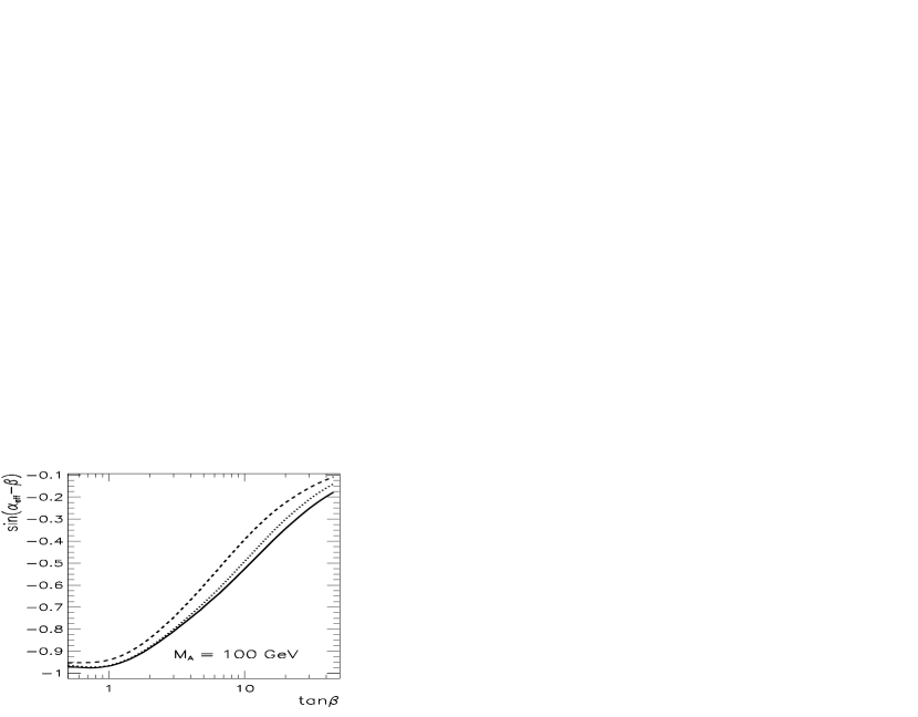
Figure 3: $\sin(\alpha_{\rm eff}-\beta)$ as a function of $\tan\beta$ (left plots) and $M_{h}$ (right plots) for $X_{t}=0$ and the parameters of Table 1. The solid line represents the two-loop FD result (see eq. (27)), the dotted line shows the RG improved one-loop EPA result, and the dashed line shows the one-loop FD result.

3.3 Results for the cross sections

Differences in the Higgs-production cross sections between our FD result (containing the complete one-loop result and the dominant two-loop corrections) and the RG $\alpha_{\rm eff}$ approximation have a two-fold origin: the different predictions for the values of $M_{h}$ and $\alpha_{\rm eff}$, which we compared in the previous section, and the additional contributions contained in the FD result (i.e. the one-loop 3- and 4-point vertex functions and the 2-point contributions that are not contained in $\alpha_{\rm eff}$).

In Fig. 4 we present the cross sections for the two production channels for a LEP2 energy of $\sqrt{s}=206$ GeV, in the no-mixing and the maximal-mixing scenario, as a function of $\tan\beta$. Fig. 5 shows the same results as a function of $M_{h}$. At LEP2 energies, the box diagram contributions are small, of the order of 2-3% [18, 19], and do not modify the cross section behavior in a significant way.

Figure 4: $\sigma_{Zh}$ and $\sigma_{Ah}$ at $\sqrt{s}=206\,\,\mathrm{GeV}$ as a function of $\tan\beta$ for two values of $M_{A}$ and the parameters of Table 1. The upper (lower) row contains the result for the no- (maximal)-mixing scenario. The solid line represents the two-loop FD result, the dotted line shows the result for the RG $\alpha_{\rm eff}$ approximation and the dashed line shows the one-loop FD result.

Figure 5: $\sigma_{Zh}$ and $\sigma_{Ah}$ at $\sqrt{s}=206\,\,\mathrm{GeV}$ as a function of $M_{h}$ for two values of $M_{A}$ and the parameters of Table 1. The upper (lower) row contains the result for the no- (maximal)-mixing scenario. The solid line represents the two-loop FD result, the dotted line shows the result for the RG $\alpha_{\rm eff}$ approximation and the dashed line shows the one-loop FD result.

As can be seen from both figures, the cross sections for the Higgs-strahlung process corresponding to the FD result and the RG $\alpha_{\rm eff}$ approximation are close to each other, with differences of the order of a few per cent. The only exception occurs at $X_{t}\approx 0$ and large $\tan\beta$. In this case the difference can amount up to 50% when the cross sections are expressed as a function of $\tan\beta$, but is considerably reduced when they are calculated in terms of $M_{h}$. The two-loop result in the FD calculation is always above the one-loop result; the difference can be sizable, but is then mostly due to the kinematical effect that the values for $M_{h}$ at one-loop are much larger than at the two-loop level. This effect is especially pronounced at the kinematical endpoints, i.e. for large $\tan\beta$.

Associated $Ah$ production is of interest at LEP2 energies only for sufficiently low $M_{A}\leq 120$ GeV, otherwise it is kinematically forbidden. Therefore we restricted our plots for $\sigma_{Ah}$ in Figs. 4 and 5 to $M_{A}=100\,\,\mathrm{GeV}$. The difference between the FD result and the RG $\alpha_{\rm eff}$ approximation is larger than for $\sigma_{Zh}$ and may reach about 20% for not too large $\tan\beta$ values. The result of the two-loop FD calculation is mostly above the one-loop result, but the differences are much smaller than for the Higgs-strahlung process.

For both processes, the differences between the FD result and the RG $\alpha_{\rm eff}$ approximation are not particularly pronounced, however visibly larger than those induced by the modifications of $\alpha_{\rm eff}$ only. For LEP2 energies they can be attributed mostly to the vertex corrections to the $ZZh$ and $ZhA$ couplings [16].

Figure 6: $\sigma_{Zh}$ and $\sigma_{Ah}$ as a function of $X_{t}/M_{SUSY}$ for $\sqrt{s}=206\,\,\mathrm{GeV}$, $\tan\beta=5$ and the parameters of Table 1. The solid line represents the two-loop FD result, the dotted line shows the RG $\alpha_{\rm eff}$ approximation and the dashed line shows the one-loop FD result.

The dependence on the $\tilde{t}$ mixing is depicted in Fig. 6. The main effect on $\sigma_{Zh},\sigma_{Ah}$ is kinematical and arises from the change of $M_{h}$ with $X_{t}/M_{SUSY}$. This effect leads to a visible (additional) asymmetry in the two-loop FD results, whereas the RG $\alpha_{\rm eff}$ approximation and the one-loop FD result show a weaker asymmetry in $X_{t}/M_{SUSY}$. As can be seen from the figure, the differences between the methods are much larger (typically more then 10%) when associated production is considered, with the above-mentioned “kinematical” asymmetry further increased by the inclusion of the vertex corrections.

Figure 7: $\sigma_{Zh}$ and $\sigma_{Ah}$ as a function of $M_{h}$ at $\sqrt{s}=500\,\,\mathrm{GeV}$, for two values of $M_{A}$, $X_{t}/M_{SUSY}=2$, and the parameters of Table 1. The solid (dot-dashed) line represents the two-loop FD result including (excluding) box contributions, the dotted line shows the RG $\alpha_{\rm eff}$ approximation and the dashed line shows the one-loop FD result.

In Fig. 7 the cross sections for the Higgs-strahlung process and the associated production are shown for a typical Linear Collider energy, $\sqrt{s}=500$ GeV [3], in the maximal-mixing scenario (in the no-mixing scenario similar results have been obtained). In addition to the previous plots we also show the result for the two-loop FD calculation where the box contributions have not been included, in order to point out their relative importance for high-energy collisions. For $\sqrt{s}=500\,\,\mathrm{GeV}$ the differences between the FD result and the RG $\alpha_{\rm eff}$ approximation are larger than in the low-energy scenario, an effect that is more pronounced for the higher value of $M_{A}$. For $M_{A}=200\,\,\mathrm{GeV}$, typically they are of the order of 10-15% for $\sigma_{Zh}$ and even up to 25% for $\sigma_{Ah}$ (for $M_{h}\;\raisebox{-3.00003pt}{$\stackrel{{\scriptstyle\displaystyle>}}{{\sim}}$}\;90\,\,\mathrm{GeV}$). The difference between the two-loop and one-loop FD result can be sizable. The two-loop result for $\sigma_{Zh}$ is in general larger than the one-loop value, again increasing with $M_{A}$, where for $M_{A}=200\,\,\mathrm{GeV}$ the difference can amount up to 15%. $\sigma_{Ah}$, on the other hand, is decreased at the two-loop level for $M_{A}=200\,\,\mathrm{GeV}$ and the difference may be sizable.

The box contributions become more important for higher $\sqrt{s}$ and change the total cross section by 5-10%. This result remains unchanged even if sleptons are significantly heavier than $M_{\tilde{l}}=300$ GeV used in our numerical analysis, as the dominant contributions to box diagrams are given by $W$ and Higgs boson exchanges [18, 19], which do not depend on $M_{\tilde{l}}$. Also, one should recall that box contributions lead to an angular distribution of the final-state particles different from the effective Born approximation and thus give much larger corrections to the differential rather than to the total cross section, at least for some range of the scattering angle. Therefore, the box diagrams have a significant effect at Linear Collider energies and thus have to be included. The same conclusions can be drawn for $\sqrt{s}=500\,\,\mathrm{GeV}$ in the no-mixing scenario, which we do not show here. The differences between the FD result and the RG $\alpha_{\rm eff}$ approximation are only slightly smaller than in the maximal-mixing case.

Figure 8: $\sigma_{Zh}$ and $\sigma_{Ah}$ as a function of $\sqrt{s}$ for $\tan\beta=5$, $X_{t}=0$, and the parameters of Table 1. The solid (dot-dashed) line represents the two-loop FD result including (excluding) box contributions, the dotted line shows the RG $\alpha_{\rm eff}$ approximation and the dashed line shows the one-loop FD result.

Figure 9: $\sigma_{Zh}$ and $\sigma_{Ah}$ as a function of $M_{A}$ at $\sqrt{s}=500\,\,\mathrm{GeV}$, shown for $\tan\beta=5$ and $\tan\beta=50$, $X_{t}=0$, and the parameters of Table 1. The solid (dot-dashed) line represents the two-loop FD result including (excluding) box contributions, the dotted line shows the RG $\alpha_{\rm eff}$ approximation and the dashed line shows the one-loop FD result.

In Fig. 8 the results for $\sigma_{Zh}$ and $\sigma_{Ah}$ are shown as a function of $\sqrt{s}$ in the no-mixing scenario for $M_{A}=100,200\,\,\mathrm{GeV}$. Besides the obvious kinematical drop-off of the cross sections, one can observe that the relative differences between the FD two-loop result and the RG $\alpha_{\rm eff}$ approximation grow with $\sqrt{s}$. The differences remain almost constant or even increase slowly in absolute terms, whereas the full cross sections decrease. $\sigma_{Ah}$ becomes very small for large $M_{A}$, as can be seen in more detail in Fig. 9. There we show the dependence of $\sigma_{Zh}$ and $\sigma_{Ah}$ on $M_{A}$ in the no-mixing scenario for $\tan\beta=5$ and $\tan\beta=50$. For $\sigma_{Zh}$, the $A$ boson decouples quickly; the dependence on $M_{A}$ becomes very weak for $M_{A}\;\raisebox{-3.00003pt}{$\stackrel{{\scriptstyle\displaystyle>}}{{\sim}}$}\;250\,\,\mathrm{GeV}$, when $\sigma_{Zh}$ is already practically constant (compare e.g. Ref. [13]). In the same limit, $\sigma_{Ah}$ goes quickly to zero due to suppression of the effective $ZhA$ coupling, which is $\sim\cos(\alpha_{\rm eff}-\beta)$; also the kinematical suppression plays a role, but this becomes significant only for sufficiently large $M_{A}$, $M_{A}>350\,\,\mathrm{GeV}$. For large $\tan\beta$ the decoupling of $M_{A}$ is even more rapid. The differences between the FD two-loop result and the RG $\alpha_{\rm eff}$ approximation for the Higgs-strahlung cross section tend also to a constant, but they increase with $M_{A}$ for the associated production. The latter can be explained by the growing relative importance of 3- and 4-point vertex function contributions compared to the strongly suppressed Born-like diagrams. As can be seen from Fig. 9, for $\tan\beta=50$ and $M_{A}\geq 300\,\,\mathrm{GeV}$ the FD two-loop result is almost an order of magnitude larger than the result of the RG $\alpha_{\rm eff}$ approximation, and starts to saturate. This can be attributed to the fact that the (non-decoupling) vertex and box contributions begin to dominate the cross section value. However, such a situation occurs only for very small $\sigma_{Ah}$ values, $\sigma_{Ah}\approx 10^{-3}$ fb, below the expected experimental LC sensitivities.

4 Conclusions

Using the Feynman-diagrammatic approach we have calculated the production cross sections for $e^{+}e^{-}\to hZ,hA$. The Higgs-boson propagator corrections have been evaluated, including besides the full one-loop result also the dominant and subdominant two-loop corrections. In addition we have included also the full set of one-loop vertex and box corrections.

We have also investigated an improved Born approximation based on the effective mixing angle, $\alpha_{\rm eff}$, in the neutral ${\cal CP}$-even Higgs sector. We have shown analytically that this approximation corresponds to taking into account the Higgs-boson propagator corrections with neglected external momentum at one-loop and two-loop order.

While the previous results available in the literature neglected the large two-loop corrections in the case of the Feynman-diagrammatic approach and were restricted to an improved Born approximation in the case of the renormalization-group improved one-loop Effective Potential approach, our new result combines the dominant two-loop corrections with the complete Feynman-diagrammatic one-loop result and thus represents the presently most precise prediction for the production cross sections for $e^{+}e^{-}\to hZ,hA$.

Specifically we have numerically analyzed the effect of the two-loop contributions incorporated in our result, which turned out to be sizable. We have furthermore compared our full Feynman-diagrammatic results for $\sigma_{Zh}$ and $\sigma_{Ah}$ with the approximation where $\alpha_{\rm eff}$ and $M_{h}$ are evaluated within the renormalization-group improved one-loop Effective Potential approach (RG $\alpha_{\rm eff}$ approximation). For LEP2 energies, $\sqrt{s}=206\,\,\mathrm{GeV}$, the difference between the Feynman-diagrammatic result and the RG $\alpha_{\rm eff}$ approximation stays mostly at the per cent level in the parameter space allowed by the LEP2 exclusion limits for $M_{h}$. At energies reachable at an $e^{+}e^{-}$ linear collider, e.g. $\sqrt{s}=500\,\,\mathrm{GeV}$, the difference between the Feynman-diagrammatic result and the RG $\alpha_{\rm eff}$ approximation can reach 10-15% for $\sigma_{Zh}$ or even 25% for $\sigma_{Ah}$. The box contributions play an important role for high $\sqrt{s}$ and can amount up to 10%. Therefore in a precision analysis for a high energy $e^{+}e^{-}$ collider the two-loop propagator corrections as well as the complete diagrammatic one-loop contributions should be included.

Appendix Appendix  Explicit expressions for the cross sections

Performing the sum over polarization states in eq. (23) one gets for the associated scalar and pseudoscalar production:

$${\cal A}_{1PS}^{i}=-~{}{\cal A}_{2PS}^{i}={e^{2}\over 8}{\lambda}^{2}\left(s,M^{2}_{A},M^{2}_{H_{i}}\right)\left(\left|a^{i}_{PS}\right|^{2}+\left|b^{i}_{PS}\right|^{2}\right),$$ (A.1)

where

$$a^{i}_{PS} = \hat{c}_{V}\left(2\tilde{V}^{(0)i1}_{ZPS}+\tilde{F}_{P}^{i1}+\tilde{F}_{S}^{i1}\right)-2\tilde{V}^{(0)i1}_{ZPS}{\hat{\Sigma}^{T}_{\gamma Z}(s)\over D_{\gamma}(s)}+\left({\tilde{G}}_{P}^{i1}+{\tilde{G}}_{S}^{i1}\right){D_{Z}(s)\over D_{\gamma}(s)},$$

$$b^{i}_{PS} = \hat{c}_{A}\left(2\tilde{V}^{(0)i1}_{ZPS}+\tilde{F}_{P}^{i1}+\tilde{F}_{S}^{i1}\right),$$ (A.2)

and $\lambda$ as given in eq. (22). The corresponding expressions for the Higgs-strahlung process are more complicated:

$${\cal A}_{2ZS}^{i} = -{e^{2}{\lambda}^{2}\left(s,M^{2}_{Z},M^{2}_{H_{i}}\right)\over 32M_{Z}^{2}}\times$$ (A.3)

$$\times \left[\left|2a^{i}_{ZS}-\left(s+M^{2}_{Z}-M^{2}_{H_{i}}\right)b^{i}_{ZS}\right|^{2}-4sM_{Z}^{2}\left|b^{i}_{ZS}\right|^{2}+\right.$$

$$+ \left.\left|2c^{i}_{ZS}-\left(s+M^{2}_{Z}-M^{2}_{H_{i}}\right)d^{i}_{ZS}\right|^{2}-4sM_{Z}^{2}\left|d^{i}_{ZS}\right|^{2}\right],$$

$${\cal A}_{1ZS}^{i}=e^{2}s\left(\left|a^{i}_{ZS}\right|^{2}+\left|c^{i}_{ZS}\right|^{2}\right)-{\cal A}_{2ZS}^{i},$$ (A.4)

where

$$a^{i}_{ZS} = \hat{c}_{V}\left(\tilde{V}^{(0)i}_{ZZS}+\tilde{F}_{1}^{i}\right)-\tilde{V}^{(0)i}_{ZZS}{\hat{\Sigma}^{T}_{\gamma Z}(s)\over D_{\gamma}(s)}+{\tilde{G}}_{1}^{i}{D_{Z}(s)\over D_{\gamma}(s)},$$

$$b^{i}_{ZS} = \hat{c}_{V}\left(\tilde{F}_{3}^{i}-\tilde{F}_{4}^{i}\right)+\left({\tilde{G}}_{3}^{i}-{\tilde{G}}_{4}^{i}\right){D_{Z}(s)\over D_{\gamma}(s)},$$

$$c^{i}_{ZS} = \hat{c}_{A}\left(\tilde{V}^{(0)i}_{ZZS}+\tilde{F}_{1}^{i}\right),$$

$$d^{i}_{ZS} = \hat{c}_{A}\left(\tilde{F}_{3}^{i}-\tilde{F}_{4}^{i}\right).$$ (A.5)

The quantities $\tilde{F}$ and $\tilde{G}$ denote effective Higgs–gauge-boson vertex form factors. They can be defined as follows. At the tree level the relevant Higgs-boson vertices read (the assignment of momenta is given in Sect. 2.4):

$$V^{(0)\mu\nu i}_{ZZS}=iV^{(0)i}_{ZZS}~{}g^{\mu\nu},$$ (A.6)

$$V^{(0)\mu ij}_{ZPS}=V^{(0)ij}_{ZPS}\left(p~{}-~{}q\right)^{\mu},$$ (A.7)

where $V^{(0)i}_{ZZS}$ and $V^{(0)ij}_{ZPS}$ can be written in matrix form as (index $j$ numerates CP-odd Higgs bosons: $A\equiv P_{1}$, $G\equiv P_{2}$):

$$V^{(0)i}_{ZZS}={eM_{Z}\over s_{W}c_{W}}\left(\begin{array}[]{r}\cos(\alpha-\beta)\\ -\sin(\alpha-\beta)\end{array}\right),$$ (A.10)

$$V^{(0)ij}_{ZPS}=-{e\over 2s_{W}c_{W}}\left(\begin{array}[]{rr}\sin(\alpha-\beta)&\cos(\alpha-\beta)\\ \cos(\alpha-\beta)&-\sin(\alpha-\beta)\end{array}\right).$$ (A.13)

After including one-loop vertex corrections the renormalized vertices have the form:

$$V^{\mu ij}_{ZPS}=p^{\mu}\left(V^{(0)ij}_{ZPS}+\hat{F}_{P}^{ij}\right)-q^{\mu}\left(V^{(0)ij}_{ZPS}+\hat{F}_{S}^{ij}\right),$$ (A.14)

$$V^{\mu\nu i}_{ZZS}=i\left[g^{\mu\nu}\left(V^{(0)i}_{ZZS}+\hat{F}^{i}_{1}\right)+p^{\mu}p^{\nu}\hat{F}^{i}_{2}+q^{\mu}q^{\nu}\hat{F}^{i}_{3}+p^{\mu}q^{\nu}\hat{F}^{i}_{4}+q^{\mu}p^{\nu}\hat{F}^{i}_{5}\right],$$ (A.15)

where $\hat{F}_{a}$’s are the renormalized vertex form factors.

Next, we define the respective quantities with tilde which are obtained by inclusion of the one-loop corrections on the external lines. For instance, the complete vertices read (in the following: $i^{\prime}=3-i,j^{\prime}=3-j$.):

$$\tilde{V}^{ij}_{ZPS} = \left({\cal Z}^{\rm ext}_{{\rm S\,}i}{\cal Z}^{\rm ext}_{{\rm P\,}j}\right)^{1/2}\left(V^{ij}_{ZPS}+{\cal Z}^{\rm mix}_{{\rm S\,}i}V^{i^{\prime}j}_{ZPS}+{\cal Z}^{\rm mix}_{{\rm P\,}j}V^{ij^{\prime}}_{ZPS}+{\cal Z}^{\rm mix}_{{\rm S\,}i}{\cal Z}^{\rm mix}_{{\rm P\,}j}V^{i^{\prime}j^{\prime}}_{ZPS}\right),$$ (A.16)

and

$$\tilde{V}^{i}_{ZZS}=\left({\cal Z}^{\rm ext}_{Z}{\cal Z}^{\rm ext}_{{\rm S\,}i}\right)^{1/2}\left(V^{i}_{ZZS}+{\cal Z}^{\rm mix}_{{\rm S\,}i}V^{i^{\prime}}_{ZZS}\right),$$ (A.17)

where

$${\cal Z}^{\rm ext}_{Z}=\mbox{Re}\,\left(1+{\partial\over\partial q^{2}}\left.\hat{\Sigma}^{T}_{Z}(q^{2})\right|_{q^{2}=M_{Z}^{2}}\right)^{-1}.$$ (A.18)

The vertices $\tilde{V}_{ZPS},\tilde{V}_{ZZS}$ can be decomposed into $\tilde{V}^{(0)}_{ZPS},\tilde{F}_{P},\tilde{F}_{S}$ etc. (as in eq. (A.14,A.15)) where e.g. $\tilde{F}^{i}_{1}=\left({\cal Z}_{Z}^{\rm ext}{\cal Z}^{\rm ext}_{{\rm S\,}i}\right)^{1/2}\left(F^{i}_{1}+{\cal Z}^{\rm mix}_{{\rm S\,}i}F^{i^{\prime}}_{1}\right)$ etc.

To include photon exchange in the $s$-channel one needs to know also the renormalized vertices $V_{\gamma PS}$ and $V_{\gamma ZS}$ (which vanish at the tree level):

$$V^{\mu ij}_{\gamma PS}=p^{\mu}\hat{G}_{P}^{ij}-q^{\mu}\hat{G}_{S}^{ij},$$ (A.19)

$$V^{\mu\nu i}_{\gamma ZS}=i\left[g^{\mu\nu}\hat{G}^{i}_{1}+p^{\mu}p^{\nu}\hat{G}^{i}_{2}+q^{\mu}q^{\nu}\hat{G}^{i}_{3}+p^{\mu}q^{\nu}\hat{G}^{i}_{4}+q^{\mu}p^{\nu}\hat{G}^{i}_{5}\right].$$ (A.20)

The vertices $\tilde{V}_{\gamma PS},\tilde{V}_{\gamma ZS}$ are defined similarly as shown in eqs. (A.16, A.17).

The explicit expressions for the one-loop corrections to the vertices $V_{ZPS}$, $V_{ZZS}$, $V_{\gamma PS}$ and $V_{\gamma ZS}$ can be found in Ref. [16].

References

-
[1]
G. Kane, C. Kolda and J. Wells,
Phys. Rev. Lett. 70 (1993) 2686,
hep-ph/9210242;
J. Espinosa and M. Quirós, Phys. Rev. Lett. 81 (1998) 516, hep-ph/9804235. -
[2]
P. Igo-Kemenes, talk given at the LEPC meeting,
3rd of November 2000;
The ALEPH collaboration, Phys. Lett. B 495 (2000) 1, hep-ex/0011045;
The DELPHI collaboration, CERN-EP 2001-004, to appear in Phys. Lett. B;
The L3 collaboration, Phys. Lett. B 495 (2000) 18, hep-ex/0011043;
The OPAL collaboration, to appear in Phys. Lett. B, hep-ex/0101014. -
[3]
R. Brinkmann et al. (editors), Conceptual
Design of a 500 GeV Linear Collider with Integrated X-ray
Laser Facility, DESY 97-048;
see also: TESLA TDR, obtainable from www.desy.de/lcnotes/tdr/ . - [4] A. Djouadi, W. Kilian, M. Mühlleitner and P.M. Zerwas, Eur. Phys. Jour. C 10 (1999) 45, hep-ph/9903229.
-
[5]
H. Haber and R. Hempfling,
Phys. Rev. Lett. 66 (1991) 1815;
Y. Okada, M. Yamaguchi and T. Yanagida, Prog. Theor. Phys. 85 (1991) 1;
J. Ellis, G. Ridolfi and F. Zwirner, Phys. Lett. B 257 (1991) 83; Phys. Lett. B 262 (1991) 477;
R. Barbieri and M. Frigeni, Phys. Lett. B 258 (1991) 395. - [6] M. Carena, J. Espinosa, M. Quirós and C. Wagner, Phys. Lett. B 355 (1995) 209, hep-ph/9504316.
- [7] M. Carena, M. Quirós and C. Wagner, Nucl. Phys. B 461 (1996) 407, hep-ph/9508343.
- [8] H. Haber, R. Hempfling and A. Hoang, Z. Phys. C 75 (1997) 539, hep-ph/9609331.
- [9] R. Hempfling and A. Hoang, Phys. Lett. B 331 (1994) 99, hep-ph/9401219.
- [10] R.-J. Zhang, Phys. Lett. B 447 (1999) 89, hep-ph/9808299.
- [11] J. Espinosa and R.-J. Zhang, JHEP 0003 (2000) 026, hep-ph/9912236; Nucl. Phys. B 586 (2000) 3, hep-ph/0003246.
- [12] S. Heinemeyer, W. Hollik and G. Weiglein, Phys. Rev. D 58 (1998) 091701, hep-ph/9803277; Phys. Lett. B 440 (1998) 296, hep-ph/9807423.
- [13] S. Heinemeyer, W. Hollik and G. Weiglein, Eur. Phys. Jour. C 9 (1999) 343, hep-ph/9812472.
- [14] W. Kilian, M. Krämer and P.M. Zerwas, Phys. Lett. B 373 (1996) 135, hep-ph/9512335.
- [15] P.H. Chankowski, S. Pokorski and J. Rosiek, Phys. Lett. B 274 (1992) 191; Phys. Lett. B 286 (1992) 307.
- [16] P.H. Chankowski, S. Pokorski and J. Rosiek, Nucl. Phys. B 423 (1994) 437; Nucl. Phys. B 423 (1994) 497.
- [17] A. Dabelstein, Z. Phys. C 67 (1995) 495, hep-ph/9409375.
- [18] V. Driesen and W. Hollik, Z. Phys. C 68 (1995), 485, hep-ph/9504335.
- [19] V. Driesen, W. Hollik and J. Rosiek, Z. Phys. C 71 (1996) 259, hep-ph/9512441.
- [20] J. Gunion, H. Haber, G. Kane and S. Dawson, The Higgs Hunter’s Guide, Addison-Wesley, 1990.
-
[21]
A. Djouadi, J. Kalinowski and P.M. Zerwas,
Z. Phys. C 57 (1993) 569;
S. Dittmaier, M. Krämer, Y. Liao, M. Spira and P.M. Zerwas, Phys. Lett. B 441 (1998) 383, hep-ph/9808433; Phys. Lett. B 478 (2000) 247, hep-ph/0002035;
S. Dawson and L. Reina, Phys. Rev. D 57 (1998) 5851, hep-ph/9712400; Phys. Rev. D 59 (1999) 054012, hep-ph/9808443; Phys. Rev. D 61 (2000) 013002, hep-ph/9906419. - [22] P. Janot, in Physics at LEP2, eds. G. Altarelli, T. Sjöstrand and F. Zwirner, CERN 96-01, Vol. 2, p. 309.
- [23] P. Janot and A. Quadt, private communication.
- [24] A. Pilaftsis and C.E.M. Wagner, Nucl. Phys. B 553 (1999) 3, hep-ph/9902371.
- [25] S. Heinemeyer, W. Hollik and G. Weiglein, Eur. Phys. Jour. C 16 (2000) 139, hep-ph/0003022.
-
[26]
The two-loop corrections are contained in
FeynHiggs and FeynHiggsFast:
S. Heinemeyer, W. Hollik and G. Weiglein, Comp. Phys. Comm. 124 2000 76, hep-ph/9812320; hep-ph/0002213.
A public Fortran code for the production cross sections is in preparation. All codes are accessible via www.feynhiggs.de. - [27] S. Heinemeyer, W. Hollik and G. Weiglein, Phys. Lett. B 455 (1999) 179, hep-ph/9903404.
- [28] S. Heinemeyer, W. Hollik and G. Weiglein, JHEP 0006 (2000) 009, hep-ph/9909540; hep-ph/9912263.
- [29] M. Carena, S. Heinemeyer, C. Wagner and G. Weiglein, hep-ph/9912223.
- [30] M. Carena, H. Haber, S. Heinemeyer, W. Hollik, C. Wagner and G. Weiglein, Nucl. Phys. B 580 (2000) 29, hep-ph/0001002.
-
[31]
S. Andringa et al.,
Searches for Higgs Bosons: Preliminary Combined Results using
LEP Data Collected at Energies up to 209 GeV, ALEPH 2000-074 CONF
2000-051, DELPHI 2000-148 CONF 447, L3 Note 2600, OPAL Technical
Note TN661;
A. Dedes, S. Heinemeyer, P. Teixeira-Dias and G. Weiglein, Jour. Phys. G 26 (2000) 582, hep-ph/9912249.