LBNL-47430

UCB-PTH-01/03

hep-ph/yymmddd

The Role of Wino Content in Neutralino Dark Matter

Andreas Birkedal-Hansen and Brent D. Nelson

Theoretical Physics Group
Ernest Orlando Lawrence Berkeley National Laboratory
University of California, Berkeley, California 94720
and
Department of Physics
University of California, Berkeley, California 94720

We investigate the dark matter prospects of supersymmetric models with nonuniversal gaugino masses. We find that for very particular values of the ratio of soft supersymmetry-breaking gaugino masses, $M_{2}/M_{1}$, an enhanced coannihilation efficiency between the lightest chargino and the lightest neutralino occurs, allowing for scalars with masses well above the normally accepted limits for viable dark matter in the universal case. As a specific example, we investigate models of hidden sector gaugino condensation. These models exhibit high scalar masses, previously thought dangerous, and the requisite freedom in the ratio of gaugino masses. The cosmologically viable regions of parameter space are investigated, allowing very specific statements to be made about the content of the supersymmetry-breaking hidden sector.

Disclaimer

This document was prepared as an account of work sponsored by the United States Government. Neither the United States Government nor any agency thereof, nor The Regents of the University of California, nor any of their employees, makes any warranty, express or implied, or assumes any legal liability or responsibility for the accuracy, completeness, or usefulness of any information, apparatus, product, or process disclosed, or represents that its use would not infringe privately owned rights. Reference herein to any specific commercial products process, or service by its trade name, trademark, manufacturer, or otherwise, does not necessarily constitute or imply its endorsement, recommendation, or favoring by the United States Government or any agency thereof, or The Regents of the University of California. The views and opinions of authors expressed herein do not necessarily state or reflect those of the United States Government or any agency thereof of The Regents of the University of California and shall not be used for advertising or product endorsement purposes.

Lawrence Berkeley Laboratory is an equal opportunity employer.

It has long been held that one of the prime virtues of supersymmetry as an explanation of the hierarchy problem is that it tends to also provide a solution to the dark matter problem as a nearly automatic consequence of R-parity conservation. The lightest supersymmetric particle (LSP) is then stable and, as it tends to be a neutral gaugino, it will typically have the right mass and annihilation rate in the early universe to provide sufficient mass density today to account for observations suggesting $\rho_{\rm tot}\simeq\rho_{\rm crit}$ [1].

This paper initially investigates the dark matter implications of the most widely studied benchmark in supersymmetric phenomenology, the constrained Minimal Supersymmetric Standard Model (cMSSM). We emphasize that the cMSSM fails to solve the dark matter problem over most of its parameter space with the exception of certain very special patterns of soft supersymmetry-breaking terms. These patterns must constrain the neutralino (a fermion) to have a very specific mass relationship to an unrelated boson such as the lightest Higgs or the stau. Barring these fine-tuned relationships, the cMSSM predicts too much dark matter – thus bringing it into conflict with direct measurements of the age of the universe [2, 3]. We find this failure to be due, in part, to the cMSSM constraint on the gaugino mass ratio $M_{2}/M_{1}$. Eliminating this assumption of universal gaugino masses uncovers new regions of parameter space that allow for cosmologically allowed, and often experimentally preferred, values of the neutralino relic density.

This paper is organized as follows: in Section 1 we present our methodology in the context of the cMSSM with its standard minimal supergravity (mSUGRA) universal soft supersymmetry-breaking terms. Subsequently, in Section 2, we relax our assumption of universal gaugino masses. While the relic density implications of nonuniversal gaugino masses, and in particular the role of $M_{2}/M_{1}$ in dark matter phenomenology, have been explored previously these past studies have either focused on specific models or have not included the important effects of coannihilation between the LSP and the lightest chargino [4, 5].

In Section 3 we consider a specific class of supergravity models derived from heterotic string theory which implement supersymmetry breaking through gaugino condensation in a hidden sector [7, 8, 9, 10] as an example of how the general results of Section 2 can be applied on a model-by-model basis. Requiring a cosmologically relevant thermal LSP relic density will imply very specific conclusions about the content of the hidden sector of these models. Finally, we conclude and remark upon possible extensions of this work.

1 Universal Gaugino Masses

The phenomenological consequences of the cMSSM have been studied extensively [11], including the cosmological implications of its (presumed stable) LSP [12]. In such a regime the entire low energy phenomenology is specified by five parameters: a common gaugino mass $M_{1/2}$, a common scalar mass $M_{0}$, a common trilinear scalar A-term $A_{0}$, the value of $\tan\beta$ and the sign of the $\mu$-parameter in the scalar potential. These values are defined at some high energy scale, typically taken to be the scale of gauge coupling unification $\Lambda_{\rm UV}\sim 2\times 10^{16}$ GeV.

To obtain the superpartner spectrum at the electroweak scale the renormalization group equations (RGEs) are run from the boundary scale to the electroweak scale [13]. In the following, all gauge and Yukawa couplings as well as A-terms were run with one loop RGEs while scalar masses and gaugino masses were run at two loops to capture the possible effects of heavy scalars and a heavy gluino on the evolution of third generation squarks and sleptons. We chose to keep only the top, bottom and tau Yukawas and the corresponding A-terms.

At the electroweak scale $\Lambda_{\rm EW}=M_{Z}$ the one loop corrected effective potential $V_{\rm 1-loop}=V_{\rm tree}+\Delta V_{\rm rad}$ is computed and the effective $\mu$-term $\bar{\mu}$ is calculated

$${\bar{\mu}}^{2}=\frac{\left(m_{H_{d}}^{2}+\delta m_{H_{d}}^{2}\right)-\left(m_{H_{u}}^{2}+\delta m_{H_{u}}^{2}\right)\tan{\beta}}{\tan^{2}{\beta}-1}-\frac{1}{2}M_{Z}^{2}.$$ (1)

In equation (1) the quantities $\delta m_{H_{u}}$ and $\delta m_{H_{d}}$ are the second derivatives of the radiative corrections $\Delta V_{\rm rad}$ with respect to the up-type and down-type Higgs scalar fields, respectively. These corrections include the effects of all third generation particles. If the right hand side of equation (1) is positive then there exists some initial value of $\mu$ at the high energy scale which results in correct electroweak symmetry breaking with $M_{Z}=91.187$ GeV.

The neutralino states and their masses are calculated using the neutralino mass matrix

$$\left(\begin{array}[]{cccc}M_{1}&0&-\sin\theta_{W}\cos\beta M_{Z}&\sin\theta_{W}\sin\beta M_{Z}\\ 0&M_{2}&\cos\theta_{W}\cos\beta M_{Z}&-\cos\theta_{W}\sin\beta M_{Z}\\ -\sin\theta_{W}\cos\beta M_{Z}&\cos\theta_{W}\cos\beta M_{Z}&0&-\mu\\ \sin\theta_{W}\sin\beta M_{Z}&-\cos\theta_{W}\sin\beta M_{Z}&-\mu&0\end{array}\right),$$ (2)

where $M_{1}$ is the mass of the hypercharge U(1) gaugino at the electroweak scale and $M_{2}$ is the mass of the SU(2) gauginos at the electroweak scale. The matrix (2) is given in the $(\tilde{B},\tilde{W},\tilde{H}^{0}_{d},\tilde{H}^{0}_{u})$ basis, where $\tilde{B}$ represents the bino, $\tilde{W}$ represents the neutral wino and $\tilde{H}^{0}_{d}$ and $\tilde{H}^{0}_{u}$ are the down-type and up-type Higgsinos, respectively.

The lightest eigenvalue of this matrix is then typically the LSP and it is overwhelmingly bino-like in content over most of the parameter space when $\tan\beta$ is low. This is because the cMSSM universality constraint on gaugino masses at the high scale of the theory implies $M_{1}\simeq\frac{1}{2}M_{2}$ when the masses are evolved to the electroweak scale via the RGEs. Provided $|M_{1}|,|M_{2}|\ll|\mu|$, which is the case for low $\tan\beta$, the LSP mass is then dominated by $M_{1}$ and has a typical bino content of $\mathrel{\hbox to0.0pt{\raise 2.15277pt\hbox{$>$}\hss}{\lower 2.15277pt\hbox{$\sim$}}}99$%. We will restrict ourselves to this low $\tan\beta$ regime and adopt a value of $\tan\beta=3$ for the remainder of the paper. The dark matter prospects of the high $\tan\beta$ limit have been studied recently by Feng et al. [15].

More generally the content of the LSP can be parametrized by writing the lightest neutralino as:

$$\chi^{0}_{1}=N_{11}\tilde{B}+N_{12}\tilde{W}+N_{13}\tilde{H}^{0}_{d}+N_{14}\tilde{H}^{0}_{u},$$ (3)

which is normalized to $N_{11}^{2}+N_{12}^{2}+N_{13}^{2}+N_{14}^{2}=1$. Thus by saying that the bino content of the lightest neutralino is high, we mean $N_{11}\simeq 1$.

Given the particle spectrum we compute the thermal relic LSP density with a modified version of the software package neutdriver [16]. This program includes all of the annihilation processes computed by Drees and Nojiri [17] which are used to compute a thermally averaged cross section $<\sigma v>_{\rm ann}$ and freeze-out temperature $x_{F}=T_{F}/m_{\chi^{0}_{1}}$. From knowledge of the mass of the lightest neutralino $m_{\chi^{0}_{1}}$ (assumed to be the LSP), $<\sigma v>_{\rm ann}$ and $T_{F}$, a relic abundance can be computed using the standard approximation [16]

$$\Omega_{\chi}h^{2}=\frac{1.07\times 10^{9}x_{F}}{g_{*}^{1/2}M_{\rm Pl}\left(a_{\rm eff}+3\left(b_{\rm eff}-a_{\rm eff}/4\right)/x_{F}\right)}{\rm GeV}^{-1},$$ (4)

where we have expressed the thermally averaged annihilation cross section as an expansion in powers of the relative velocity:

$$<\sigma v>_{\rm ann}=a_{\rm eff}+b_{\rm eff}v^{2}+...$$ (5)

A proper determination of relic LSP densities requires that the above computation be amended to include the possible effects of coannihilation [18]. This occurs when another particle is only slightly heavier than the lightest neutralino so that both particles freeze out of equilibrium at approximately the same temperature. The neutralino can now not only deplete its relic abundance through annihilation processes such as $\chi^{0}_{1}\chi^{0}_{1}\rightarrow e^{+}e^{-}$, but also through interactions with the coannihilator such as $\chi^{\pm}_{1}\chi^{0}_{1}\rightarrow e^{\pm}\nu_{e}$. The extreme importance of including relevant coannihilation channels has recently been emphasized for the case of the cMSSM [19, 20], and in that spirit we have added a number of coannihilation channels which are relevant for both the universal gaugino mass case [20] as well as the case of nonuniversal gaugino masses to be considered in Section 2.

The program neutdriver includes $\chi^{\pm}\chi^{0}_{1}$ coannihilation to $W^{\pm}\gamma$ [4] and two (massless) fermions $f\bar{f}^{\prime}$ which we recalculated to account for non-zero fermion masses. We have also included a calculation of the process $\chi^{\pm}\chi^{0}_{1}\rightarrow W^{\pm}Z$, and found this channel to often dominate when kinematically accessible. Additionally, we have inserted the results of [19] for $\chi^{0}_{1}\tilde{\tau}$ coannihilation to $Z\tau$, $\gamma\tau$, $h\tau$, and $H\tau$ final states.

The region of cMSSM parameter space that gives rise to acceptable levels of bino-like LSP relic density is given in Figure 1 where we have plotted contours of $\Omega_{\chi}{\rm h}^{2}=0.1$, $0.3$ and $\Omega_{\chi}{\rm h}^{2}=1$. Here $\Omega_{\chi}$ is the fractional LSP matter density relative to the critical density and $h$ is the reduced Hubble parameter: $h\simeq 0.65$ [21]. We have chosen $M_{1/2}$ and $M_{0}$ as free parameters in the manner of Ellis, Falk & Olive [20] with $\tan\beta=3$, $A_{0}=0$ and positive $\mu$-term.

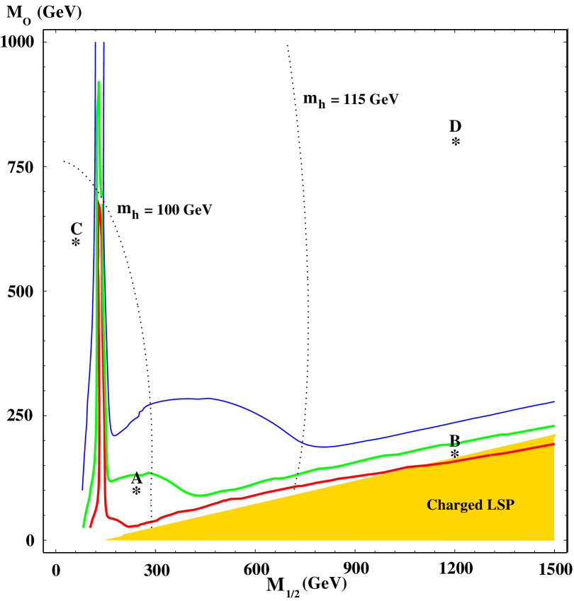
Figure 1: Preferred Dark Matter Region for cMSSM. Contours of $\Omega_{\chi}{\rm h}^{2}$ of 0.1 (bottom-most contour), 0.3 and 1.0 (top-most contour) are given. The shaded region is ruled out by virtue of having the stau as the LSP. The Higgs pole region and stau coannihilation tail are clearly discernible. We have also added contours of constant Higgs mass for $m_{h}=100$ GeV and $m_{h}=115$ GeV. The four labeled points are examined in Figure 2.

This plot is similar to the ones presented in [20] and we reproduce it here to draw attention to two important facts. First, observations suggest that the preferred values for cold dark matter densities are in the range $0.1\leq\Omega_{\chi}{\rm h}^{2}\leq 0.3$ [22], though including the latest evidence of a cosmological constant [3] may shift this to $0.06\mathrel{\hbox to0.0pt{\raise 2.15277pt\hbox{$<$}\hss}{\lower 2.15277pt\hbox{$\sim$}}}\Omega_{\chi}{\rm h}^{2}\mathrel{\hbox to0.0pt{\raise 2.15277pt\hbox{$<$}\hss}{\lower 2.15277pt\hbox{$\sim$}}}0.2$. This experimental data points to a region of the cMSSM parameter space in which both the universal scalar mass and the universal gaugino mass are small, on the order of $200$ GeV for each (see, for example, the region around point A in Figure 1). In fact, heavy scalars can only be accommodated cosmologically if nature was kind enough to arrange the soft-supersymmetry breaking parameters so that the mass of the LSP is about half of the mass of the lightest Higgs boson. In that case, though t-channel scalar fermion exchange may be suppressed and the annihilation rate into two fermions is not sufficient to deplete the LSP density adequately, the annihilation through resonant s-channel exchange of the lightest Higgs is efficient enough to provide an acceptable dark matter region insensitive to the scalar mass.

We have allowed our $M_{0}$ value to range to as much as a TeV, in contrast to [20], to accentuate the point that most of the cMSSM parameter space considered “natural” in the literature predicts far too much neutralino relic density. Every point in Figure 1 above the $\Omega_{\chi}{\rm h}^{2}=0.3$ line is already excluded by astrophysical measurements of the dark matter density. This rules out almost all of the plotted parameter space except for the low-mass region including point A and the thin strip right above the region excluded due to a charged LSP (the region including point B). Once we begin to impose constraints arising from Higgs searches at LEP, the preferred low mass region in Figure 1 begins to be ruled out. The only region which then remains in the $\{M_{0},M_{1/2}\}$ plane for $\tan\beta=3$ is that which is due to coannihilation between the LSP and the lightest stau. Being in this region requires a very specific relationship between the gaugino mass parameter and the unrelated scalar mass parameter.

To better illustrate the physics behind Figure 1 and to serve as a comparison for our subsequent analysis we have chosen four representative points from the parameter space for deeper investigation. Both points A and B fall within the cosmologically preferred region. Point B is in the coannihilation ’tail,’ so we would expect most of the annihilation cross section to come from coannihilation. As we can see in Figure 2 the annihilation cross section of point B is indeed dominated by coannihilation. We can also see the importance of t-channel sfermion exchange to $\chi^{0}\chi^{0}\rightarrow f\bar{f}$ in points A and B, which is due to the universal scalar mass being relatively light so that this channel is open. Referring back to Figure 1, both points C and D are in regions where there is too much relic density. Figure 2 shows that, indeed, the annihilation is too inefficient to eliminate enough dark matter. The annihilation channels to two fermions still dominate but now sfermion exchange is too suppressed to provide the critical annihilation rate (indicated by the dashed line). As with points C and D, most of the parameter space of the cMSSM is experimentally excluded since there is no efficient way of depleting the relic density.

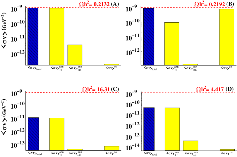
Figure 2: Annihilation Cross Sections for Selected Points from Figure 1. These graphs detail the composition of the neutralino depletion cross section. The total depletion cross section is on the far left. The next two columns divide the normal annihilation channels by final state into two fermions or all other annihilation channels. The final column is the sum of all coannihilation channels. The total relic density is given at the top of each plot and the dashed horizontal line illustrates the ideal total depletion cross section for an $\Omega_{\chi}h^{2}=0.2$.

It is a generic result of the low $\tan\beta$ cMSSM scenario that, excluding stau coannihilation, cosmological viability depends almost solely on the t-channel exchange of sfermions. This strict dependence causes most of the presumed parameter space to be experimentally excluded, leaving the dark matter prospects of the cMSSM in serious jeopardy.

2 Nonuniversal Gaugino Masses

The reason for the failure of the low $\tan\beta$ cMSSM to solve the dark matter problem is the low annihilation cross section for the neutralino. The only channel capable of providing a suitable cross section is the aforementioned t-channel sfermion exchange which is only efficient in a small region of parameter space. If we relax the GUT relationship between the gaugino masses but still remain in the large $|\mu|$ limit (low $\tan\beta$) then we will continue to have a predominantly gaugino-like LSP ($N_{11}^{2}+N_{12}^{2}\simeq 1$) with the relative values of $N_{11}$ and $N_{12}$ governed by the relative values of $M_{1}$ and $M_{2}$. Decreasing $M_{2}$ relative to $M_{1}$ at the electroweak scale increases the wino content of the LSP until ultimately $M_{1}\gg M_{2}$ and $N_{11}\simeq 0$, $N_{12}\simeq 1$.

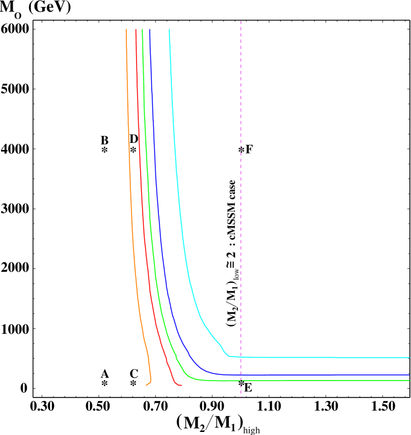
Figure 3: Preferred Dark Matter Region for Nonuniversal Gaugino Masses. Contours of $\Omega_{\chi}{\rm h}^{2}$ of 0.01, 0.1, 0.3, 1.0 and 10.0 from left to right, respectively, are given as a function of the ratio of SU(2) to U(1) gaugino masses $M_{2}/M_{1}$ at the high scale. The cMSSM is recovered where the two masses are equal at the high scale, as has been indicated by the dashed line. The six labeled points are examined in Figure 4.

The bino component of the neutralino couples with a U(1) gauge strength whereas the wino component couples with the larger SU(2) gauge strength, thus enhancing its annihilation cross section and thereby lowering its relic density. As $N_{12}$ is increased more parameter space should open up for dark matter until annihilation becomes too efficient in the pure wino-like limit and we are left with no neutralino dark matter at all [6]. This is evident in Figure 3 where we plot contours of $\Omega_{\chi}{\rm h}^{2}$ as a function of scalar mass and the ratio $\left(M_{2}/M_{1}\right)$ at the boundary condition scale $\Lambda_{\rm GUT}$. Allowing the gaugino masses to vary independently introduces two new degrees of freedom. We have chosen to vary the ratio $\left(M_{2}/M_{1}\right)$ while fixing the value of $M_{1/2}\equiv{\rm min}\left(M_{1},M_{2}\right)$ and $M_{3}$ at the high scale. In practice we use our choice of $M_{1/2}$ to determine the value of the smaller of the pair $\left(M_{1},M_{2}\right)$ at the high scale and then use the ratio $\left(M_{2}/M_{1}\right)$ to determine the larger of $\left(M_{1},M_{2}\right)$. In Figure 3 we have set $M_{1/2}=200$ GeV and $M_{3}=M_{1/2}$.

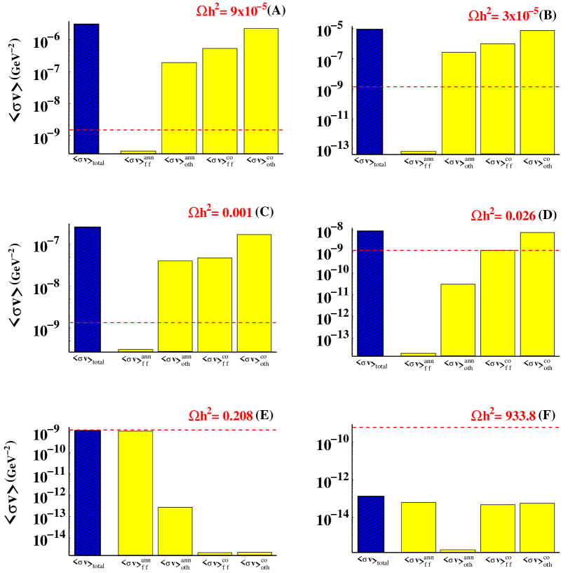
Figure 4: Annihilation Cross Sections for Selected Points from Figure 3. These graphs are identical in layout to those of Figure 2, except now the coannihilation channels are split into two columns: two-fermion final states and everything else.

Particular values of $\left(M_{2}/M_{1}\right)$ which deviate from the universal cMSSM case allow for cosmologically interesting relic densities which are almost independent of the scalar mass. To see how dark matter physics changes as one departs from the cMSSM we have analyzed the six labelled points from Figure 3 in Figure 4. Starting with the two cMSSM points, E and F, the importance of the process $\chi^{0}_{1}\chi^{0}_{1}\rightarrow f\bar{f}$ is again demonstrated. Point F has scalars that are too heavy for the two fermion final state to sufficently deplete the LSP relic density while point E has much lighter scalars, allowing efficient annihilation to two fermions and resulting in an appropriate amount of dark matter. Given the value of $M_{1/2}=200$ GeV for this plot point E would lie a little to the left of point A in Figure 1.

Points C and D sit at much lower values of $\left(M_{2}/M_{1}\right)$, resulting in a lightest chargino that is much more degenerate with the lightest neutralino. This enhances the importance of coannihilation channels, leading them to dominate the annihilation cross section. The main channels for coannihilation are $\chi^{\pm}\chi^{0}_{1}\rightarrow f\bar{f}^{\prime}$, making up the left-hand coannihilation column in Figure 4, and $\chi^{\pm}\chi^{0}_{1}\rightarrow W^{\pm}Z$, which is the main contributor to the right-hand coannihilation column. Chargino-neutralino coannihilation has become so efficient here that the relic density is now not enough to account for observations. It should be noted that point D gives almost the cosmologically preferred relic density – its relic density is higher than that of point C for two reasons. First, the mass of the lightest neutralino drops slightly in going from point D ($\sim 122$ GeV) to point C ($\sim 112$ GeV). Second, the lower scalar mass at point C allows t-channel exchange of scalar fermions to go unsuppressed. This is important in one of the diagrams contributing to $\chi^{\pm}\chi^{0}_{1}\rightarrow f\bar{f}^{\prime}$. The wino content of the lightest neutralino is also increased by lowering $\left(M_{2}/M_{1}\right)$, causing the standard annihilation channel to two fermions to become relatively unimportant. This increase in efficiency continues through points A and B, now making the neutralino relic density cosmologically irrelevant.

The irrelevance of scalar masses above $1$ TeV can be simply understood. Above $1$ TeV the t-channel scalar exchange contribution to $\chi^{0}_{1}\chi^{0}_{1}\rightarrow f\bar{f}$ is suppressed due to the scalar mass. With enhanced wino content, however, channels that were previously suppressed are now more efficient, such as $\chi^{0}_{1}\chi^{0}_{1}\rightarrow W^{+}W^{-}$. More importantly, we can also see from Figure 3 that much of the parameter space in the $\{M_{0},\left(M_{2}/M_{1}\right)\}$ plane is not ruled out: an $\Omega_{\chi}h^{2}\leq 0.1$ is not experimentally excluded, it just does not completely explain all of the needed dark matter.

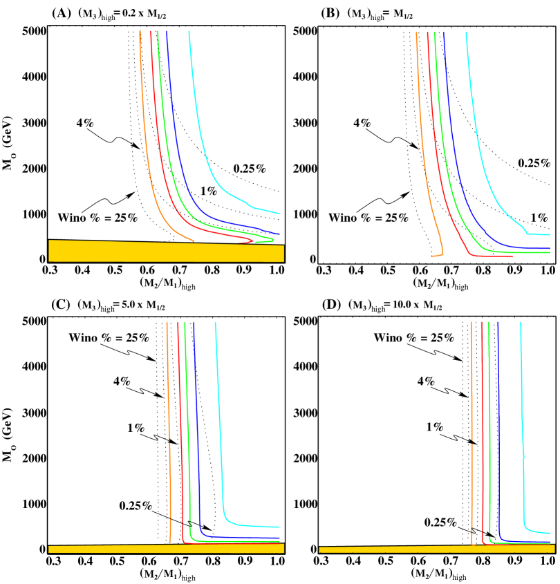
Figure 5: Preferred Dark Matter Region with Nonuniversal Gaugino Masses for Various $M_{3}$ Values I. Contours of constant relic density are given by the solid lines for $\Omega_{\chi}{\rm h}^{2}=$ 0.01, 0.1, 0.3, 1, and 10 from left to right. The dotted lines are curves of constant wino content for $N_{12}^{2}$ = 0.25, 0.04, 0.01 and 0.025 from left to right. The value of the high-scale gluino mass $M_{3}$ is given in terms of the universal gaugino mass $M_{1/2}$ at the top of each plot. This plot uses a value of $M_{1/2}=200$ GeV except for panel (A) where $M_{1/2}=250$ GeV. The shaded region is excluded by the constraints of Table 1.

Table 1: Superpartner and Higgs mass constraints imposed [23, 24].

Gluino Mass		$m_{\tilde{g}}$	$>$	$190$ GeV
Lightest Neutralino Mass		$m_{\chi^{0}_{1}}$	$>$	$32.5$ GeV
Lightest Chargino Mass		$m_{\chi_{1}^{\pm}}$	$>$	$75$ GeV
Lightest Squark Masses		$m_{\tilde{q}}$	$>$	$90$ GeV
Lightest Slepton Masses		$m_{\tilde{l}}$	$>$	$87$ GeV
Light Higgs Mass		$m_{h}$	$>$	$95.3$ GeV
Pseudoscalar Higgs Mass		$m_{A}$	$>$	$84.1$ GeV
Charged Higgs Mass		$m_{H^{\pm}}$	$>$	$69.0$ GeV

Figure 5 examines the effect of changing the boundary scale value of $M_{3}$ on the cosmologically preferred parameter space of Figure 3. In Figure 5 and subsequent plots we impose the constraint that the LSP be electrically neutral and that the resulting spectrum at the electroweak scale satisfies the search limits of Table 1. The shaded region in panel (A) of Figure 5 is excluded by the gluino mass bound while the shaded region in panels (C) and (D) are excluded by the constraint on the stau mass. As the value of the gluino mass $M_{3}$ is increased relative to the other gaugino masses the cosmologically preferred range of the ratio $\left(M_{2}/M_{1}\right)$ moves to slightly higher values.

It is apparent from Figure 6 that the crucial variable in the determination of the LSP relic density is the value of the ratio $\left(M_{2}/M_{1}\right)$ at the electroweak scale. The region of preferred relic density $0.1\leq\Omega_{\chi}{\rm h}^{2}\leq 0.3$ consistently asymptotes to the region between the values $\left(M_{2}/M_{1}\right)_{\rm low}=1.15$ and $\left(M_{2}/M_{1}\right)_{\rm low}=1.25$ independent of the value of $M_{3}$, with the influence of the universal scalar mass $M_{0}$ most pronounced for small values of $M_{3}$. Most of the reason for this behavior is the composition of the low-scale squark masses. For large values of $M_{3}$ the RG evolution of the squark masses is dominated by $M_{3}$ which drives scalar masses to higher values and further suppresses the t-channel slepton and squark exchange diagrams. This causes the asymptotic approach to scalar-mass-independence to saturate for much lower values of $M_{0}$ than in the low $M_{3}$ case, where the value of squark and slepton masses is largely independent of $M_{3}$ and merely a function of the boundary value $M_{0}$ at the high scale.

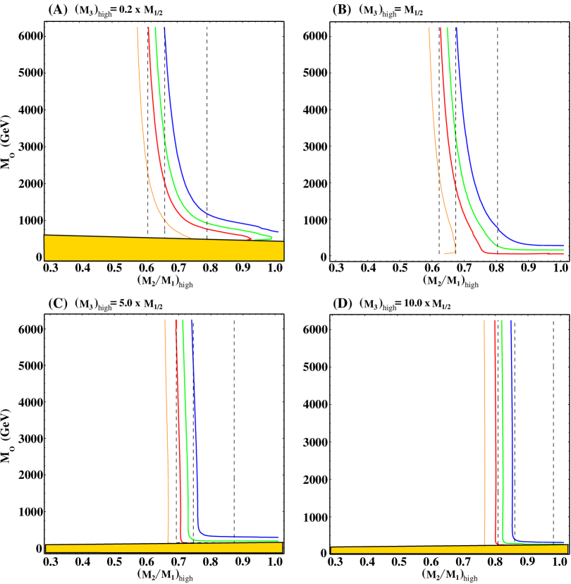
Figure 6: Preferred Dark Matter Region with Nonuniversal Gaugino Masses for Various $M_{3}$ Values II. Contours of constant relic density are given by the solid lines for $\Omega_{\chi}{\rm h}^{2}=$ 0.01, 0.1, 0.3, and 1.0 from left to right. The value of the ratio $\left(M_{2}/M_{1}\right)_{\rm low}$ is indicated by the dashed lines for the values $\left(M_{2}/M_{1}\right)_{\rm low}=$ 1.15, 1.25 and 1.50 from left to right. The shaded regions are ruled out because of a stau LSP.

These results are robust under changes in the relative sign between the soft supersymmetry-breaking values of $M_{1,2}$ and $M_{3}$, as well as changes in the overall gaugino mass scale $M_{1/2}$, as is demonstrated in Figure 7.  For low values of $M_{3}$ there is little difference between the positive and negative values, though for high values of $M_{3}$ the entire plot moves from right to left when the sign is reversed. Nonetheless, the cosmologically preferred region falls between the same values of $\left(M_{2}/M_{1}\right)_{\rm low}$ (denoted by dashed lines), regardless of the sign of $M_{3}$: it is only the preferred region of $\left(M_{2}/M_{1}\right)_{\rm high}$ that changes with the sign flip. Both the effects of the magnitude of $M_{3}$ as well as its relative sign can be understood from the effect $M_{3}$ has on the running of $M_{2}$ and $M_{1}$, starting at two loops. The two loop running of the gaugino masses, in the conventions of [13], is partially given by

$$\frac{d}{dt}M_{a}\ni\frac{2g_{a}^{2}}{\left(16\pi^{2}\right)^{2}}\sum_{b=1}^{3}B_{ab}^{\left(2\right)}g_{b}^{2}\left(M_{a}+M_{b}\right),$$ (6)

where $B_{ab}^{\left(2\right)}$ is a matrix of positive entries. Therefore the higher the value of $|M_{3}|$ the greater the impact on the gaugino masses $M_{1}$ and $M_{2}$. Furthermore, this effect is felt more strongly by the SU(2) gaugino mass than the U(1) gaugino mass. Thus for a given value of $\left(M_{2}/M_{1}\right)_{\rm high}$ changing the sign of $M_{3}$ drives the value of $M_{2}$ higher at the electroweak scale to a greater degree than it does $M_{1}$, resulting in a higher value of $\left(M_{2}/M_{1}\right)_{\rm low}$. This in turn leads to an increased relic density as can be seen by comparing the right and left sets of panels in Figure 7.

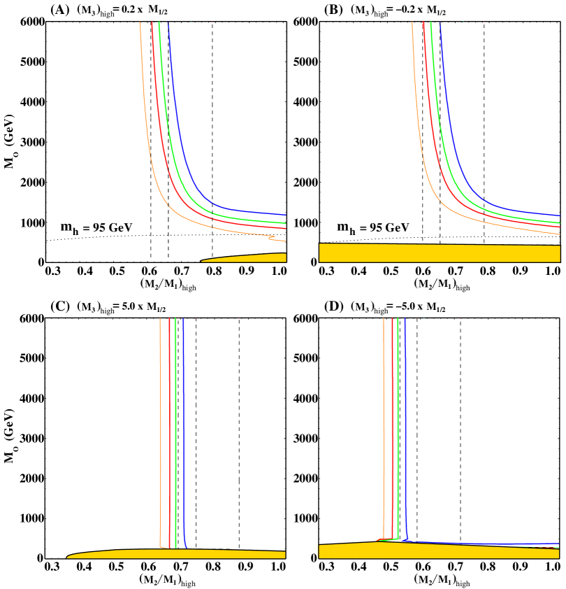
Figure 7: Preferred Dark Matter Region with Nonuniversal Gaugino Masses for Differing Signs of $M_{3}$. The solid lines are lines of constant $\Omega_{\chi}{\rm h}^{2}$ and the dashed lines represent values of $\left(M_{2}/M_{1}\right)_{low}=$ 1.15, 1.25 and 1.50 as in Figure 6. The shaded regions are excluded by virtue of having a stau for the LSP. We have indicated the Higgs mass constraint in panels (A) and (B). Here $M_{1/2}$ is taken to be 500 GeV in all panels.

We have seen that relaxing the GUT constraint on the gaugino masses allows for significant improvement in the dark matter arena. This relaxation only requires a slight increase in the wino content of the LSP on the order of 0.1 to 5% (see Figure 5): the LSP is still predominantly bino-like and is not in the unappealling wino-dominated scenario which must rely on other mechanisms to generate supersymmetric dark matter [25]. The observations made in this section indicate that models which allow control over $\left(M_{2}/M_{1}\right)$ at the boundary scale may be more suitable to providing supersymmetric dark matter than the unified cMSSM paradigm. In fact, requiring a cosmologically relevant relic LSP density may in turn shed light on the nature of physics at the GUT scale in models of supersymmetry breaking. We will carry out an example of just such an investigation in the next section on a class of supergravity models derived from heterotic string theory.

3 BGW Model

In this section we turn our attention to a class of heterotic string-derived supergravity theories that invoke gaugino condensation in a hidden sector to break supersymmetry. The framework for this model was first put forward by Binétruy, Gaillard and Wu [7, 8] and its phenomenology was considered in subsequent papers [9, 10]. As a supergravity model with a unification scale, many of the typical results of mSUGRA continue to hold – in particular the few number of parameters necessary to determine the low-energy spectrum. However, a newly-emphasized contribution to the gaugino masses resulting from the superconformal anomaly [26] gives a correction to the standard gaugino mass unification that has been investigated recently [27, 28]. Thus in this model one is able to determine the ratio $\left(M_{2}/M_{1}\right)$ as a function of the parameters of the hidden sector.

The soft supersymmetry-breaking gaugino masses $M_{a}$ in the BGW model are determined at the scale of gaugino condensation (typically of order $\Lambda_{\rm cond}\sim 10^{14}$ GeV). They are proportional to the gravitino mass $M_{3/2}$ and depend on the value of the beta-function coefficient of the condensing gauge group(s) of the hidden sector. In practice the soft supersymmetry-breaking terms are dominated by the condensing group with the largest beta-function coefficient, which we label $b_{+}$:

$$M_{a}\left(\mu_{c}\right)=\frac{g_{a}^{2}\left(\Lambda_{\rm cond}\right)}{2}\left(\frac{3b_{+}\left(1+b^{\prime}_{a}\ell\right)}{1+b_{+}\ell}-3b_{a}\right)M_{3/2},$$ (7)

with

$$b_{+}=\frac{1}{8\pi^{2}}\left(C_{+}-\frac{1}{3}\sum_{A}C_{+}^{A}\right).$$ (8)

Here $C_{+}$ and $C_{+}^{A}$ are the quadratic Casimirs of the adjoint and matter representations $\Phi^{A}$, respectively, under the largest condensing gauge group. In equation (7) $\ell$ is the dilaton field whose vacuum expectation value determines the string coupling constant at the string scale: $<\ell>=g_{\rm str}^{2}/2$. Here we have assumed the standard string coupling suggested by GUT scale unification: $g_{str}^{2}=0.5$. Finally, the constants $b_{a}$ and $b_{a}^{\prime}$ in (7) depend on the group theory parameters of the observable sector gauge groups. For example the SU(2) gaugino mass depends on the constants:

$$b_{2} = \frac{1}{8\pi^{2}}\left(C_{SU\left(2\right)}-\frac{1}{3}\sum_{A}C_{SU\left(2\right)}^{A}\right)$$

$$b^{\prime}_{2} = \frac{1}{8\pi^{2}}\left(C_{SU\left(2\right)}-\sum_{A}C_{SU\left(2\right)}^{A}\right),$$ (9)

with similar definitions for the SU(3) and U(1) gaugino masses. Thus the key variable $\left(M_{2}/M_{1}\right)$ depends on the value of $b_{+}$:

$$\frac{M_{2}\left(\Lambda_{\rm cond}\right)}{M_{1}\left(\Lambda_{\rm cond}\right)}=\frac{g_{2}^{2}\left(\Lambda_{\rm cond}\right)}{g_{1}^{2}\left(\Lambda_{\rm cond}\right)}\frac{\left(1+b^{\prime}_{2}\ell\right)-(b_{2}/b_{+})\left(1+b_{+}\ell\right)}{\left(1+b^{\prime}_{1}\ell\right)-(b_{1}/b_{+})\left(1+b_{+}\ell\right)}$$ (10)

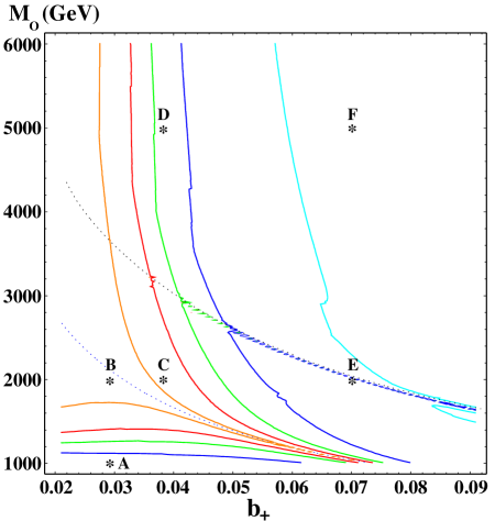
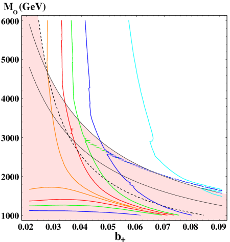
Figure 8: Preferred Region in the BGW Model. In the left panel contours of constant relic density are given as a function of $M_{0}$ and $b_{+}$ by the solid lines while the Higgs resonance and $W^{\pm}$ resonance are indicated by the upper and lower dotted lines, respectively. Moving outward from the lower dotted line are contours of $\Omega_{\chi}{\rm h}^{2}=$ 0.01, 0.1, 0.3, 1.0 and 10. In the right panel these contours are reproduced with experimental constraints from Table 1. The shaded region is excluded: the dashed curve represents a 190 GeV gluino mass while the two parallel solid curves represent a 75 GeV and a 90 GeV chargino mass from bottom to top. The labeled points are examined in detail in Figure 9.

Figure 8 shows contours of constant LSP relic density for the BGW model in the $\{b_{+},M_{0}\}$ plane, where $M_{0}$ is the usual universal scalar mass whose value is given by $M_{0}=M_{3/2}$ in the model we will consider here. While the axes of Figure 8 are very similar to those of Figures 3, 5 and 6 there are some notable differences in the BGW model. The gluino mass parameter $M_{3}$ relates to $M_{2}$ and $M_{1}$ through an identical relationship to Equation (10) and therefore changes with $b_{+}$. In the previous figures $M_{3}$ was held constant at the high scale within a single plot, but in Figure 8 the ratio $M_{3}/M_{1}$ at the condensation scale varies from 0.2 at $b_{+}=0.02$ to 0.8 at $b_{+}=0.09$. Nevertheless, there is still a region of viable dark matter largely independent of the universal scalar mass, as in the general nonuniversal cases studied in Section 2, for the same reasons: a smaller value of $\left(M_{2}/M_{1}\right)$ for lower $b_{+}$ results in higher wino content as well as more degeneracy between the lightest neutralino and chargino, resulting in conannihilation.

In the left plot of Figure 8 it is evident that this is not a result of the masses being tuned to sit on a pole. The Higgs pole, given by the locus of points for which $2m_{\chi_{1}^{0}}=m_{h}$, is indicated by the uppermost dotted line. More important is the $W$-pole, denoted by the second lower dotted line in the left plot, where a neutralino and chargino go to an on-shell $W$-boson, severely warping the lower part of the plot. However, both of these resonant regions are excluded experimentally by the criteria of Table 1 as indicated in the right plot of Figure 8 by the shaded region. The key constraints include the gluino mass (given by the dashed line) and the chargino mass (given by two parallel solid curves representing a chargino mass of 75 and 90 GeV from bottom to top).

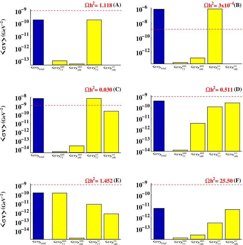
Figure 9: Annihilation Cross Sections for Selected Points From Figure 8. These graphs are identical in nature to those of Figure 4.

As with the previous cases the additonal physics contained in this plot is easily seen through a few representative points given in more detail in Figure 9. Starting from the top right in Figure 8, point F sits at far too high a value of $M_{0}$ for the normal cMSSM annihilation channels to be effective. Its high value of $b_{+}$ also gives a high value of $\left(M_{2}/M_{1}\right)_{\rm low}$ (between 1.3 and 1.4), so the wino content of the LSP is low. The dominant channels are neutralino-chargino coannihilation but this is not sufficient to deplete the relic density to acceptable levels. Point E lies exactly on the pole for two neutralinos going to an on-shell Higgs which then naturally decays to two fermions, making this the dominant final state. A lowered sfermion mass scale also allows coannihilation to two fermions to increase. Nevertheless, the net effect is still too small to bring the relic density down far enough.

Point D is in the region where one would not expect much annihilation to fermions, but for this $b_{+}$ value the neutralino and chargino are becoming more degenerate, increasing coannihilation and bringing the relic density down towards the cosmologically preferred region. Additionally, points D and F are the only two points which kinematically allow $\chi^{\pm}\chi^{0}\rightarrow W^{\pm}Z$. Once this channel is open it is the main determining factor in the relic density.

Points B and C both lie near the region where the masses of the lightest chargino and the LSP add up to exactly the mass of the charged $W$-boson. This enhances the efficiency of most channels of chargino-neutralino coannihilation, resulting in a relic density that is now a little too low to account for astrophysical observations. For point A, by contrast, the particles are off-shell so these processes are too inefficient and the relic density is too high. Note that for points A, B and C the value of the lightest chargino mass is below the experimental limit so these points are excluded.

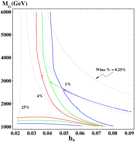
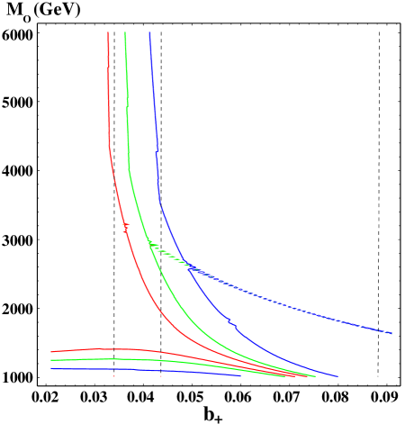
Figure 10: Preferred Region in the BGW Model. Contours of constant relic density are given as in Figure 8 by the solid lines for $\Omega_{\chi}{\rm h}^{2}=$ 0.1, 0.3, and 1.0 only. The left plot gives dotted lines of constant wino content (25%, 4%, 1%, 0.25% from left to right). The right plot gives dashed lines of constant ratio $\left(M_{2}/M_{1}\right)_{\rm low}$ (1.15, 1.25, 1.5 from left to right).

Figure 10 shows how the parameters of the BGW model determine wino content and the ratio $\left(M_{2}/M_{1}\right)_{\rm low}$. As in the case of Figures 5 and 6 from Section 2, cosmological observations favor a mild wino content of 0.1 to 5% and single out the region $1.15\leq\left(M_{2}/M_{1}\right)_{\rm low}\leq 1.25$. The correspondence between the value of $b_{+}$ and $\left(M_{2}/M_{1}\right)_{\rm high}$ is clear from the comparison of the right panel in Figure 10 and those of Figures 5 and 6, in particular panels (A) for lower values of $b_{+}$ and (B) for higher values.

To see the discriminatory power that cosmological considerations can have on model building we now look more deeply into the role of the hidden sector configuration in determining the pattern of soft supersymmetry-breaking terms in this class of supergravity models. The (nondynamical) gaugino condensates in the hidden sector are represented by dimension three chiral superfields $U_{a}\simeq{{\rm Tr}({\cal W}^{\alpha}{\cal W}_{\alpha})}_{a}$ where $a$ labels the condensing groups of the hidden sector: ${\cal G}_{\rm hid}=\prod_{a}{\cal G}_{a}$.

The superpotential for these low-energy effective degrees of freedom is that of Veneziano and Yankielovich [29]

$${{\cal L}}_{\rm VY}=\frac{1}{8}{\sum_{a}}{\int\mbox{d}^{4}\theta}\frac{E}{R}{U_{a}}\left[{b_{a}^{\prime}}\ln{\left(e^{-K/2}{U_{a}}\right)}+{\sum_{\alpha}}{b_{a}^{\alpha}}\ln{\left[\left({\Pi^{\alpha}}\right)^{p_{\alpha}}\right]}\right]+{\rm h.c.},$$ (11)

which is here written in the chiral U(1) superspace formalism [31]. The lagrangian involves the gauge condensates $U_{a}$, the complete Kähler potential $K$, and any possible gauge-invariant matter condensates described by chiral superfields $\Pi^{\alpha}\simeq{\prod_{A}}{\left(\Phi^{A}\right)}^{n_{\alpha}^{A}}$, where $\alpha$ runs from 1 to the number of condensates $N_{c}$. The coeffecients $b_{a}^{\prime}$, $b_{a}^{\alpha}$ are determined by demanding the correct transformation properties of the expression in (11) under chiral and conformal transformations [7, 30] and yield the following relations:

$$b_{a}\equiv b_{a}^{\prime}+{\sum_{\alpha}}b_{a}^{\alpha}=\frac{1}{8{\pi}^{2}}\left(C_{a}-\frac{1}{3}{\sum_{A}}C_{a}^{A}\right), {\displaystyle{\sum_{\alpha,A}}{b_{a}^{\alpha}}{n_{\alpha}^{A}}{p_{\alpha}}={\sum_{A}}\frac{C_{a}^{A}}{4{\pi}^{2}}},$$ (12)

which are equivalent to those of (8) and (9). The matter condensate superpotential is taken to be $W\left[\left({\Pi}^{p_{\alpha}}\right),T\right]={\sum_{\alpha}}c_{\alpha}{W_{\alpha}}\left(T\right)\left({\Pi}^{\alpha}\right)^{p_{\alpha}}$, where $T$ represents one of the three untwisted moduli chiral superfields $T^{I}$ which parameterize the size of the compactified space. The coefficient $c_{\alpha}$ is a Yukawa coefficient from the underlying theory which we presume to be ${\cal O}\left(1\right)$. Finally, we require on dimensional grounds that ${p_{\alpha}}\sum_{A}n_{\alpha}^{A}=3$ for all values of $\alpha$.

Armed with these elements of the lagrangian the equations of motion for the nondynamical condensate superfields can be solved [7, 10] and the condensation scale and gravitino mass determined. If we define the lowest components of the chiral superfields as $u_{a}=U_{a}|_{\theta=\bar{\theta}=0}\equiv{\rho}_{a}e^{i{\omega}_{a}}$ and $t_{I}\equiv T_{I}|_{\theta=\bar{\theta}=0}$ then the condensate value is given by

$${{\rho_{a}}^{2}}=e^{-2{\frac{b^{\prime}_{a}}{b_{a}}}}e^{K}e^{-\frac{2}{{b_{a}}g_{a}^{2}}}e^{\frac{b}{b_{a}}{\sum_{I}}\ln{(t^{I}+{\overline{t}}^{I})}}{\prod_{I}}\left|{\eta}\left(t^{I}\right)\right|^{\frac{4\left(b-b_{a}\right)}{b_{a}}}{\prod_{\alpha}}\left|b_{a}^{\alpha}/4c_{\alpha}\right|^{-2{\frac{b_{a}^{\alpha}}{b_{a}}}},$$ (13)

where $\eta(t^{I})$ is the Dedekind function. To disentangle the complexity of (13) it is convenient to assume that all of the matter in the hidden sector which transforms under a given subgroup ${\cal G}_{a}$ is of the same representation, such as the fundamental representation, and then make the simultaneous variable redefinition

$${\sum_{\alpha}}b_{a}^{\alpha}\equiv\left(b_{a}^{\alpha}\right)_{\rm eff}={N_{c}}b_{a}^{\rm rep}; \left({c_{\alpha}}\right)_{\rm eff}\equiv{N_{c}}\left({\prod_{\alpha=1}^{N_{c}}}c_{\alpha}\right)^{\frac{1}{N_{c}}}.$$ (14)

In the above equation $b_{a}^{\rm rep}$ is proportional to the quadratic Casimir operator for the matter fields in the common representation.

From a determination of the condensate value $\rho$ the supersymmetry-breaking scale can be found by solving for the gravitino mass, given by $M_{3/2}=\frac{1}{4}\left\langle\left|{\sum_{a}}{b_{a}}{u_{a}}\right|\right\rangle$ [7], though in practice we will replace the summation with the condensing group with the largest beta-function coefficient: $M_{3/2}=\frac{1}{4}{b_{+}}\left\langle\left|u_{+}\right|\right\rangle$. Now for given values of $\left({c_{\alpha}}\right)_{\rm eff}$ the gravitino mass can be plotted in the $\left\{b_{+},\left(b_{+}^{\alpha}\right)_{\rm eff}\right\}$ plane, as in Figure 11, where curve (a) is a contour of $M_{3/2}=100$ GeV for $\left({c_{\alpha}}\right)_{\rm eff}=10$ and curve (b) is a contour of $M_{3/2}=10$ TeV for $\left({c_{\alpha}}\right)_{\rm eff}=0.1$. The shaded region between these curves can then be thought of as the phenomenologically preferred region of hidden sector configuration space.

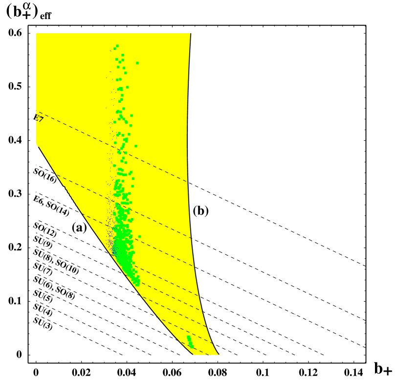
Figure 11: Preferred Dark Matter Region in Hidden Sector Configuration Space. This plot illustrates the dark matter parameter space in terms of the gauge group and matter content parameters of the hidden sector. The fine points on the left have the preferred value $0.1\leq\Omega_{\chi}{\rm h}^{2}\leq 0.3$ and the coarse points have $0.3<\Omega_{\chi}{\rm h}^{2}\leq 1.0$. The swath bounded by lines (a) and (b) is the region in which the $0.1\leq\left({c_{\alpha}}\right)_{\rm eff}\leq 10$ and the gravitino mass is between 100 GeV and 10 TeV. The dotted lines are the possible combination of gauge parameters for different hidden sector gauge groups.

Upon $Z_{N}$ orbifold compactification of the heterotic string the $E_{8}$ gauge group of the hidden sector is presumed to break to some subgroup(s) of $E_{8}$. For each such subgroup the equations in (12) define a line in the $\left\{b_{+},\left(b_{a}^{\alpha}\right)_{\rm eff}\right\}$ plane which we have displayed in Figure 11. We then sampled 25,000 combinations of $\{b_{+},\left(b_{a}^{\alpha}\right)_{\rm eff},\left({c_{\alpha}}\right)_{\rm eff}\}$ which give rise to gravitino masses between 100 GeV and 10 TeV and which yield a particle spectrum consistent with the bounds in Table 1. In Figure 11 we display those combinations which implied a relic density in the range $0.1\leq\Omega_{\chi}{\rm h}^{2}\leq 0.3$ (fine points), as well as the slightly higher range $0.3<\Omega_{\chi}{\rm h}^{2}\leq 1.0$ (coarse points).

Figure 11 clearly favors a very specific region of hidden sector parameter space with a preferred value of $b_{+}$ in the neighborhood of $b_{+}=0.036$ and a corresponding range in $\left(b_{a}^{\alpha}\right)_{\rm eff}$ of $0.2\leq\left(b_{a}^{\alpha}\right)_{\rm eff}\leq 0.6$, which points towards a large condensing group such as $SO(12)$, $SO(14)$, $SO(16)$, $E_{6}$ or $E_{7}$. A typical matter configuration for the hidden sector would be represented in Figure 11 by a point on one of the gauge group lines. The number of possible configurations consistent with a given choice of $\left\{\alpha_{\rm str},\left({c_{\alpha}}\right)_{\rm eff}\right\}$ and supersymmetry-breaking scale $M_{3/2}$ is quite restricted. For example, if we ask for a hidden sector configuration charged under the $E_{6}$ gauge group for which $C_{E_{6}}=12$ and $C_{E_{6}}^{\rm fund}=3$, and require that our matter condensates be gauge invariant so that fundamentals must come in groups of three, then from (12) the only combination that falls in the preferred region of Figure 11 is $N_{\rm fund}=9$. This combination is notable in that it was shown in [10] to possess many desirable phenomenological features. A similar analysis for the other allowed gauge groups leaves only a handful of possible hidden sector configurations, summarized in Table 2, where we have included some examples with various hidden sector effective Yukawa couplings $\left({c_{\alpha}}\right)_{\rm eff}$ and the implied values of $M_{3/2}$ and $\Omega_{\chi}{\rm h}^{2}$. As is evident from the table and from Figure 11, using the dark matter constraint on LSP relic densities is a very powerful tool in restricting the high energy physics of the underlying theory.

Table 2: Gauge group Casimirs and allowed condensate numbers.

Gauge group	$C_{a}$	$C_{a}^{\rm fund}$	$b_{a}$	$\left(b_{a}^{\alpha}\right)_{\rm eff}$	$N_{\rm fund}$	$\left({c_{\alpha}}\right)_{\rm eff}$	$M_{3/2}$ (GeV)	$\Omega_{\chi}{\rm h}^{2}$
$E_{6}$	$12$	$3$	$0.038$	$0.23$	$9$	$3.8$	$5967$	$0.633$
$SO\left(16\right)$	$14$	$1$	$0.034$	$0.29$	$34$	$2.7$	$7011$	$0.194$
$SO\left(14\right)$	$12$	$1$	$0.034$	$0.24$	$28$	$4.4$	$3383$	$0.069$
$SO\left(12\right)$	$10$	$1$	$0.034$	$0.19$	$22$	$6.3$	$1438$	$0.076$

Conclusion

The prospects for cMSSM dark matter are rapidly diminshing, barring a curious conspiracy between $M_{0}$ and $M_{1/2}$. This is due to the inefficient annihilation of a dominantly bino-like LSP. Departure from the standard cMSSM GUT relation allows values of $\left(M_{2}/M_{1}\right)$ that accomodate small admixtures of wino content for the LSP. Lowering this ratio at the electroweak scale increases the LSP annihilation efficiency by virtue of its higher wino content and the tightening degeneracy between the lightest chargino and the LSP, resulting in increased coannihilation. Ranges of $\left(M_{2}/M_{1}\right)_{\rm low}$ exist with $0.1\leq\Omega{\rm h}^{2}\leq 0.3$ and where the value of $M_{0}$ is restricted to be anything above $1$ TeV – quite in contrast to the very light scalars required in the standard cMSSM case.

The requirement of cosmologically interesting relic densities, or at least the demand that $\Omega_{\chi}{\rm h}^{2}\leq 1$, can be a powerful constraint on models with nonuniversal gaugino masses which is often quite complementary to the constraints arising from direct search limits for superpartners. As an example we investigated the BGW model of gaugino condensation derived from heterotic string theory where the number of possible hidden sector gauge groups and matter configurations could be restricted to a very small number. Similar analyses on models with small deviations from universality should prove equally fruitful. While relic densities of supersymmetric particles that were once in thermal equilibrium need not be the explanation for the missing nonbaryonic mass in the universe, it is nevertheless one of the most compelling aspects of low-energy supersymmetric phenomenology and promises to remain so even in scenarios with heavy squarks and sleptons.

References

-
[1]
H. Goldberg, Phys. Rev. Lett. 50 (1983)
1419-1422.
S. Weinberg, Phys. Rev. Lett. 50, (1983) 387-389.
J. Ellis, J. S. Hagelin, D. V. Nanopoulos, K. A. Olive and M. Srednicki, Nucl. Phys. B238 (1984) 453-476. -
[2]
P. de Bernardis et al., Nature 404 (2000) 955-959.
S. Dodelson, Int. J. Mod. Phys. A15 (2000) 2629-2644.
A. H. Jaffe et al., Cosmology from Maxima-1, Boomerang and COBE/DMR CMB Observations, astro-ph/0007333 (2000). - [3] S. Perlmutter et al., Astrophys. J. 517 (1999) 565-586.
- [4] C.-H. Chen, M. Drees and J.F. Gunion, Phys. Rev. D55 (1997) 330-347; Erratum-ibid. D60 (1999) 039901.
-
[5]
A. Corsetti and P. Nath, Gaugino Mass
Nonuniversality and Dark Matter in SUGRA, Strings and D-Brane
Models, hep-ph/0003186.
K. Griest and L. Roszkowski, Phys. Rev. D46 (1992) 3309-3317. - [6] S. Mizuta, D. Ng and M. Yamaguchi, Phys. Lett. B300 (1993) 96-103.
- [7] P. Binétruy, M. K. Gaillard and Y.-Y. Wu, Nucl. Phys. B493 (1997) 27-55.
- [8] P. Binétruy, M. K. Gaillard and Y.-Y. Wu, Nucl. Phys. B481 (1996) 109-128.
- [9] P. Binétruy, M. K. Gaillard and Y.-Y. Wu, Phys. Lett. B412 (1997) 288-295.
- [10] M. K. Gaillard and B. D. Nelson, Nucl. Phys. B571 (2000) 3-25.
-
[11]
G. L. Kane, C. Kolda, L. Roszkowski and J. D. Wells,
Phys. Rev. D49 (1994) 6173-6210.
G. L. Kane, C. Kolda, L. Roszkowski and J. D. Wells, Phys. Rev. D50 (1994) 3498-3507.
W. de Boer, H.J. Grimm, A.V. Gladyshev and D.I. Kazakov, Phys. Lett. B438 (1998) 281-289.
V. Barger et al., Report of the SUGRA Working Group for Run II of the Tevatron, hep-ph/0003154. -
[12]
M. Srednicki, R. Watkins and K. A. Olive,
Nucl. Phys. B310 (1988) 693.
K. Griest, M. Kamionkowski and M. S. Turner, Phys. Rev. D41 (1990) 3565-3582.
L. Roszkowski, Phys. Lett. B262 (1991) 59-67.
L. Roszkowski, Phys. Lett. B278 (1991) 147-154.
H. Baer and M. Brhlik, Phys. Rev. D53 (1996) 597-605.
J. Ellis and L. Roszkowski, Phys. Lett. B283 (1992) 252-260.
J. Edsjo and P. Gondolo, Phys. Rev. D56 (1997) 1879-1894.
V. Barger and C. Kao, Phys. Rev. D57 (1998) 3131-3139.
A. B. Lahanas, D. V. Nanopoulos and V. C. Spanos, Phys. Lett. B464 (1999) 213-222. - [13] S. P. Martin and M. T. Vaughn, Phys. Rev. D50 (1994) 2282-2292.
- [14] T. Ghergetta, G. Giudice and J. Wells, Nucl. Phys. B559 (1999) 27-47.
- [15] J. L. Feng, K. T. Matchev and F. Wilczek, Phys. Lett. B482 (2000) 388-399.
- [16] G. Jungman, M. Kamionkowski and K. Griest, Phys. Rept. 267 (1996) 195-373.
- [17] M. Drees and M. M. Nojiri, Phys. Rev. D47 (1993) 376-408.
-
[18]
K. Griest and D. Seckel, Phys. Rev. D43 (1991)
3191-3203.
P. Gondolo and G. Gelmini, Nucl. Phys. B360 (1991) 145-179.
S. Mizuta and M. Yamaguchi, Phys. Lett. B298 (1993) 120-126. -
[19]
J. Ellis, T. Falk, K.A. Olive and M. Srednicki,
Astropart.Phys. 13 (2000) 181-213.
J. Ellis, T. Falk and K. A. Olive, Phys. Lett. B444 (1998) 367-372. -
[20]
J. Ellis, T. Falk, K. A. Olive and M. Schmitt,
Phys. Lett. B388 (1996) 97-105.
J. Ellis, T. Falk, K. A. Olive and M. Schmitt, Phys. Lett. B413 (1997) 355-364.
J. Ellis, T. Falk, G. Ganis and K. A. Olive, Phys. Rev. D62 (2000) 075010. - [21] J. R. Primack, Cosmological Parameters 2000, astro-ph/0007187.
-
[22]
N. Bahcall, J. P. Ostriker, S. Perlmutter and
P. J. Steinhardt, Science 284 (1999) 1481-1488.
W. L. Freedman, Phys. Rept. 333-334 (2000) 13-31. - [23] Particle Data Group, Eur. Phys. J. C15 (2000) 1.
- [24] DELPHI Collaboration, Phys. Lett. B489 (2000) 38-54.
- [25] T. Moroi and L. Randall, Nucl. Phys. B570 (2000) 455-472.
-
[26]
G. F. Giudice, M. A. Luty, H. Murayama and
R. Rattazzi, JHEP 9812 (1998) 027.
L. Randall and R. Sundrum, Nucl. Phys. B557 (1999) 79-118. - [27] M. K. Gaillard, B. D. Nelson and Y.-Y. Wu, Phys. Lett. B459 (1999) 549-556.
- [28] P. Binètruy, M. K. Gaillard and B. D. Nelson, One Loop Soft Supersymmetry Breaking Terms in Superstring Effective Theories, hep-ph/0011081, to appear in Nucl. Phys. B.
-
[29]
G. Veneziano and S. Yankielowicz, Phys. Lett. B113
(1982) 231.
T. R. Taylor, G. Veneziano and S. Yankielowicz, Nucl. Phys. B218 (1983) 493. - [30] M. K. Gaillard and T. R. Taylor, Nucl. Phys. B381 (1992) 577-596.
-
[31]
P. Binétruy, G. Girardi and R. Grimm, Supergravity Couplings: A Geometric Formulation, hep-th/0005225,
to appear in Physics Reports.
P. Binétruy, G. Girardi, R. Grimm and M. Müller, Phys. Lett. B189 (1987) 83-88.