Measurement of the Inclusive Jet Cross Section in ${\bar{p}p}$ collisions at $\sqrt{s}=1.8$ TeV

Abstract

We present results from the measurement of the inclusive jet cross section for jet transverse energies from 40 to 465 GeV in the pseudo-rapidity range $0.1<|\eta|<0.7$. The results are based on 87 $pb^{-1}$ of data collected by the CDF collaboration at the Fermilab Tevatron Collider. The data are consistent with previously published results. The data are also consistent with QCD predictions given the flexibility allowed from current knowledge of the proton parton distributions. We develop a new procedure for ranking the agreement of the parton distributions with data and find that the data are best described by QCD predictions using the parton distribution functions which have a large gluon contribution at high $E_{T}$ (CTEQ4HJ).

T. Affolder,²³ H. Akimoto,⁴⁵ A. Akopian,³⁸ M. G. Albrow,¹¹ P. Amaral,⁸ S. R. Amendolia,³⁴ D. Amidei,²⁶ K. Anikeev,²⁴ J. Antos,¹ G. Apollinari,¹¹ T. Arisawa,⁴⁵ T. Asakawa,⁴³ W. Ashmanskas,⁸ F. Azfar,³¹ P. Azzi-Bacchetta,³² N. Bacchetta,³² M. W. Bailey,²⁸ S. Bailey,¹⁶ P. de Barbaro,³⁷ A. Barbaro-Galtieri,²³ V. E. Barnes,³⁶ B. A. Barnett,¹⁹ S. Baroiant,⁵ M. Barone,¹³ G. Bauer,²⁴ F. Bedeschi,³⁴ S. Belforte,⁴² W. H. Bell,¹⁵ G. Bellettini,³⁴ J. Bellinger,⁴⁶ D. Benjamin,¹⁰ J. Bensinger,⁴ A. Beretvas,¹¹ J. P. Berge,¹¹ J. Berryhill,⁸ B. Bevensee,³³ A. Bhatti,³⁸ M. Binkley,¹¹ D. Bisello,³² M. Bishai,¹¹ R. E. Blair,² C. Blocker,⁴ K. Bloom,²⁶ B. Blumenfeld,¹⁹ S. R. Blusk,³⁷ A. Bocci,³⁸ A. Bodek,³⁷ W. Bokhari,³³ G. Bolla,³⁶ Y. Bonushkin,⁶ D. Bortoletto,³⁶ J. Boudreau,³⁵ A. Brandl,²⁸ S. van den Brink,¹⁹ C. Bromberg,²⁷ M. Brozovic,¹⁰ N. Bruner,²⁸ E. Buckley-Geer,¹¹ J. Budagov,⁹ H. S. Budd,³⁷ K. Burkett,¹⁶ G. Busetto,³² A. Byon-Wagner,¹¹ K. L. Byrum,² P. Calafiura,²³ M. Campbell,²⁶ W. Carithers,²³ J. Carlson,²⁶ D. Carlsmith,⁴⁶ W. Caskey,⁵ J. Cassada,³⁷ A. Castro,³ D. Cauz,⁴² A. Cerri,³⁴ A. W. Chan,¹ P. S. Chang,¹ P. T. Chang,¹ J. Chapman,²⁶ C. Chen,³³ Y. C. Chen,¹ M. -T. Cheng,¹ M. Chertok,⁴⁰ G. Chiarelli,³⁴ I. Chirikov-Zorin,⁹ G. Chlachidze,⁹ F. Chlebana,¹¹ L. Christofek,¹⁸ M. L. Chu,¹ Y. S. Chung,³⁷ C. I. Ciobanu,²⁹ A. G. Clark,¹⁴ A. Connolly,²³ J. Conway,³⁹ M. Cordelli,¹³ J. Cranshaw,⁴¹ D. Cronin-Hennessy,¹⁰ R. Cropp,²⁵ R. Culbertson,¹¹ D. Dagenhart,⁴⁴ S. D’Auria,¹⁵ F. DeJongh,¹¹ S. Dell’Agnello,¹³ M. Dell’Orso,³⁴ L. Demortier,³⁸ M. Deninno,³ P. F. Derwent,¹¹ T. Devlin,³⁹ J. R. Dittmann,¹¹ A. Dominguez,²³ S. Donati,³⁴ J. Done,⁴⁰ T. Dorigo,¹⁶ N. Eddy,¹⁸ K. Einsweiler,²³ J. E. Elias,¹¹ E. Engels, Jr.,³⁵ R. Erbacher,¹¹ D. Errede,¹⁸ S. Errede,¹⁸ Q. Fan,³⁷ R. G. Feild,⁴⁷ J. P. Fernandez,¹¹ C. Ferretti,³⁴ R. D. Field,¹² I. Fiori,³ B. Flaugher,¹¹ G. W. Foster,¹¹ M. Franklin,¹⁶ J. Freeman,¹¹ J. Friedman,²⁴ Y. Fukui,²² I. Furic,²⁴ S. Galeotti,³⁴ A. Gallas,^(∗∗) 16 M. Gallinaro,³⁸ T. Gao,³³ M. Garcia-Sciveres,²³ A. F. Garfinkel,³⁶ P. Gatti,³² C. Gay,⁴⁷ D. W. Gerdes,²⁶ P. Giannetti,³⁴ P. Giromini,¹³ V. Glagolev,⁹ D. Glenzinski,¹¹ M. Gold,²⁸ J. Goldstein,¹¹ A. Gordon,¹⁶ I. Gorelov,²⁸ A. T. Goshaw,¹⁰ Y. Gotra,³⁵ K. Goulianos,³⁸ C. Green,³⁶ G. Grim,⁵ P. Gris,¹¹ L. Groer,³⁹ C. Grosso-Pilcher,⁸ M. Guenther,³⁶ G. Guillian,²⁶ J. Guimaraes da Costa,¹⁶ R. M. Haas,¹² C. Haber,²³ E. Hafen,²⁴ S. R. Hahn,¹¹ C. Hall,¹⁶ T. Handa,¹⁷ R. Handler,⁴⁶ W. Hao,⁴¹ F. Happacher,¹³ K. Hara,⁴³ A. D. Hardman,³⁶ R. M. Harris,¹¹ F. Hartmann,²⁰ K. Hatakeyama,³⁸ J. Hauser,⁶ J. Heinrich,³³ A. Heiss,²⁰ M. Herndon,¹⁹ C. Hill,⁵ K. D. Hoffman,³⁶ C. Holck,³³ R. Hollebeek,³³ L. Holloway,¹⁸ R. Hughes,²⁹ J. Huston,²⁷ J. Huth,¹⁶ H. Ikeda,⁴³ J. Incandela,¹¹ G. Introzzi,³⁴ J. Iwai,⁴⁵ Y. Iwata,¹⁷ E. James,²⁶ H. Jensen,¹¹ M. Jones,³³ U. Joshi,¹¹ H. Kambara,¹⁴ T. Kamon,⁴⁰ T. Kaneko,⁴³ K. Karr,⁴⁴ H. Kasha,⁴⁷ Y. Kato,³⁰ T. A. Keaffaber,³⁶ K. Kelley,²⁴ M. Kelly,²⁶ R. D. Kennedy,¹¹ R. Kephart,¹¹ D. Khazins,¹⁰ T. Kikuchi,⁴³ B. Kilminster,³⁷ B. J. Kim,²¹ D. H. Kim,²¹ H. S. Kim,¹⁸ M. J. Kim,²¹ S. H. Kim,⁴³ Y. K. Kim,²³ M. Kirby,¹⁰ M. Kirk,⁴ L. Kirsch,⁴ S. Klimenko,¹² P. Koehn,²⁹ A. Köngeter,²⁰ K. Kondo,⁴⁵ J. Konigsberg,¹² K. Kordas,²⁵ A. Korn,²⁴ A. Korytov,¹² E. Kovacs,² J. Kroll,³³ M. Kruse,³⁷ S. E. Kuhlmann,² K. Kurino,¹⁷ T. Kuwabara,⁴³ A. T. Laasanen,³⁶ N. Lai,⁸ S. Lami,³⁸ S. Lammel,¹¹ J. I. Lamoureux,⁴ J. Lancaster,¹⁰ M. Lancaster,²³ R. Lander,⁵ G. Latino,³⁴ T. LeCompte,² A. M. Lee IV,¹⁰ K. Lee,⁴¹ S. Leone,³⁴ J. D. Lewis,¹¹ M. Lindgren,⁶ T. M. Liss,¹⁸ J. B. Liu,³⁷ Y. C. Liu,¹ D. O. Litvintsev,⁸ O. Lobban,⁴¹ N. Lockyer,³³ J. Loken,³¹ M. Loreti,³² D. Lucchesi,³² P. Lukens,¹¹ S. Lusin,⁴⁶ L. Lyons,³¹ J. Lys,²³ R. Madrak,¹⁶ K. Maeshima,¹¹ P. Maksimovic,¹⁶ L. Malferrari,³ M. Mangano,³⁴ M. Mariotti,³² G. Martignon,³² A. Martin,⁴⁷ J. A. J. Matthews,²⁸ J. Mayer,²⁵ P. Mazzanti,³ K. S. McFarland,³⁷ P. McIntyre,⁴⁰ E. McKigney,³³ M. Menguzzato,³² A. Menzione,³⁴ C. Mesropian,³⁸ A. Meyer,¹¹ T. Miao,¹¹ R. Miller,²⁷ J. S. Miller,²⁶ H. Minato,⁴³ S. Miscetti,¹³ M. Mishina,²² G. Mitselmakher,¹² N. Moggi,³ E. Moore,²⁸ R. Moore,²⁶ Y. Morita,²² T. Moulik,²⁴ M. Mulhearn,²⁴ A. Mukherjee,¹¹ T. Muller,²⁰ A. Munar,³⁴ P. Murat,¹¹ S. Murgia,²⁷ J. Nachtman,⁶ V. Nagaslaev,⁴¹ S. Nahn,⁴⁷ H. Nakada,⁴³ I. Nakano,¹⁷ C. Nelson,¹¹ T. Nelson,¹¹ C. Neu,²⁹ D. Neuberger,²⁰ C. Newman-Holmes,¹¹ C.-Y. P. Ngan,²⁴ H. Niu,⁴ L. Nodulman,² A. Nomerotski,¹² S. H. Oh,¹⁰ T. Ohmoto,¹⁷ T. Ohsugi,¹⁷ R. Oishi,⁴³ T. Okusawa,³⁰ J. Olsen,⁴⁶ W. Orejudos,²³ C. Pagliarone,³⁴ F. Palmonari,³⁴ R. Paoletti,³⁴ V. Papadimitriou,⁴¹ S. P. Pappas,⁴⁷ D. Partos,⁴ J. Patrick,¹¹ G. Pauletta,⁴² M. Paulini,^(∗) 23 C. Paus,²⁴ L. Pescara,³² T. J. Phillips,¹⁰ G. Piacentino,³⁴ K. T. Pitts,¹⁸ A. Pompos,³⁶ L. Pondrom,⁴⁶ G. Pope,³⁵ M. Popovic,²⁵ F. Prokoshin,⁹ J. Proudfoot,² F. Ptohos,¹³ O. Pukhov,⁹ G. Punzi,³⁴ K. Ragan,²⁵ A. Rakitine,²⁴ D. Reher,²³ A. Reichold,³¹ A. Ribon,³² W. Riegler,¹⁶ F. Rimondi,³ L. Ristori,³⁴ M. Riveline,²⁵ W. J. Robertson,¹⁰ A. Robinson,²⁵ T. Rodrigo,⁷ S. Rolli,⁴⁴ L. Rosenson,²⁴ R. Roser,¹¹ R. Rossin,³² A. Roy,²⁴ A. Safonov,³⁸ R. St. Denis,¹⁵ W. K. Sakumoto,³⁷ D. Saltzberg,⁶ C. Sanchez,²⁹ A. Sansoni,¹³ L. Santi,⁴² H. Sato,⁴³ P. Savard,²⁵ P. Schlabach,¹¹ E. E. Schmidt,¹¹ M. P. Schmidt,⁴⁷ M. Schmitt,^(∗∗) 16 L. Scodellaro,³² A. Scott,⁶ A. Scribano,³⁴ S. Segler,¹¹ S. Seidel,²⁸ Y. Seiya,⁴³ A. Semenov,⁹ F. Semeria,³ T. Shah,²⁴ M. D. Shapiro,²³ P. F. Shepard,³⁵ T. Shibayama,⁴³ M. Shimojima,⁴³ M. Shochet,⁸ J. Siegrist,²³ A. Sill,⁴¹ P. Sinervo,²⁵ P. Singh,¹⁸ A. J. Slaughter,⁴⁷ K. Sliwa,⁴⁴ C. Smith,¹⁹ F. D. Snider,¹¹ A. Solodsky,³⁸ J. Spalding,¹¹ T. Speer,¹⁴ P. Sphicas,²⁴ F. Spinella,³⁴ M. Spiropulu,¹⁶ L. Spiegel,¹¹ J. Steele,⁴⁶ A. Stefanini,³⁴ J. Strologas,¹⁸ F. Strumia, ¹⁴ D. Stuart,¹¹ K. Sumorok,²⁴ T. Suzuki,⁴³ T. Takano,³⁰ R. Takashima,¹⁷ K. Takikawa,⁴³ P. Tamburello,¹⁰ M. Tanaka,⁴³ B. Tannenbaum,⁶ W. Taylor,²⁵ M. Tecchio,²⁶ R. Tesarek,¹¹ P. K. Teng,¹ K. Terashi,³⁸ S. Tether,²⁴ A. S. Thompson,¹⁵ R. Thurman-Keup,² P. Tipton,³⁷ S. Tkaczyk,¹¹ K. Tollefson,³⁷ A. Tollestrup,¹¹ H. Toyoda,³⁰ W. Trischuk,²⁵ J. F. de Troconiz,¹⁶ J. Tseng,²⁴ N. Turini,³⁴ F. Ukegawa,⁴³ T. Vaiciulis,³⁷ J. Valls,³⁹ S. Vejcik III,¹¹ G. Velev,¹¹ R. Vidal,¹¹ R. Vilar,⁷ I. Volobouev,²³ D. Vucinic,²⁴ R. G. Wagner,² R. L. Wagner,¹¹ N. B. Wallace,³⁹ A. M. Walsh,³⁹ C. Wang,¹⁰ M. J. Wang,¹ T. Watanabe,⁴³ D. Waters,³¹ T. Watts,³⁹ R. Webb,⁴⁰ H. Wenzel,²⁰ W. C. Wester III,¹¹ A. B. Wicklund,² E. Wicklund,¹¹ T. Wilkes,⁵ H. H. Williams,³³ P. Wilson,¹¹ B. L. Winer,²⁹ D. Winn,²⁶ S. Wolbers,¹¹ D. Wolinski,²⁶ J. Wolinski,²⁷ S. Wolinski,²⁶ S. Worm,²⁸ X. Wu,¹⁴ J. Wyss,³⁴ A. Yagil,¹¹ W. Yao,²³ G. P. Yeh,¹¹ P. Yeh,¹ J. Yoh,¹¹ C. Yosef,²⁷ T. Yoshida,³⁰ I. Yu,²¹ S. Yu,³³ Z. Yu,⁴⁷ A. Zanetti,⁴² F. Zetti,²³ and S. Zucchelli³

(CDF Collaboration)

I Introduction

Measurement of the inclusive jet cross section is a fundamental test of QCD predictions. The Fermilab $p\bar{p}$ collider, with $\sqrt{s}$ = 1.8 TeV, provides the highest energy collisions of any accelerator and the energies of the resulting jets cover the widest range of any experiment. Comparison of the inclusive jet cross section to predictions provides information about parton distribution functions (PDF’s) and the strong coupling constant, $\alpha_{s}$, for jet energies from 40 - 465 GeV where the jet cross section changes by 10 orders of magnitude. At the highest jet $E_{T}$, this measurement probes a distance scale of the order of $10^{-17}$ cm and has traditionally been used to search for new physics.

In this paper we present a new measurement of the inclusive differential cross-section for jet production at $\sqrt{s}$ = 1.8 TeV with the CDF detector[1]. Our previous measurement of the inclusive cross section[2] using the Run 1A data sample, (19.5 pb^-1 collected during 1992-1993), showed a significant excess of the data over the available theoretical predictions at high $E_{T}$. With substantially smaller data samples, measurements [3, 4] of the inclusive jet cross section prior to the Run 1A result found good agreement with QCD predictions and provided the best limits on quark compositeness [5]. The Run 1A result motivated a reevaluation of the theoretical uncertainties from the PDF’s [6, 7] and the derivation of a new PDF which specifically gave higher weight to the high $E_{T}$ CDF data points [8]. The measurement presented in this report uses the 87 pb^-1[9] Run 1B data sample (1994-1995) which is more than 4.5 times larger than for our previous result[2]. Comparisons are made to improved theoretical predictions and to the results of the D0 Collaboration[10].

The paper is organized as follows: Section II provides a discussion of the components of the theoretical predictions and a historical review of previous jet measurements. Sections III and IV describe the CDF detector and the data sample selection respectively. In Section V the energy calibration and corrections to the data are presented. A discussion of the systematic uncertainties follows in Section VI. Section VII describes comparison of this data to previous results. Section VIII presents quantitative estimates of the theoretical uncertainties and Section IX shows comparisons of the data to the predictions. The paper is concluded in Section X.

II Inclusive Jet Cross Sections

The suggestion that high energy hadron collisions would result in two jets of particles with the same momentum as the scattered partons [11] spawned an industry of comparisons between experimental measurements and theoretical predictions. The initial searches at the ISR ($\sqrt{s}$ = 63 GeV), provided hints of two-jet structure [12]. Extraction of a jet signal was difficult because the sharing of the hadron momentum between the constituent partons reduced the effective available parton scattering energy and the remnants of the incident hadrons produced a background of low transverse energy particles. The first clear observation of two jet structure came at a collision energy of $\sqrt{s}$ = 540 GeV at the CERN $Sp\bar{p}S$ collider [13, 14] along with the first measurements of the inclusive jet cross section. An increased data sample and improved triggering also led to the measurement of the inclusive jet cross section at the ISR [15].

Following these early results, improvements in accelerators produced both increased sample sizes and increased collision energies. Higher energy collisions produce jets of higher energy particles. This facilitates separation of jet particles from the remnants of the initial hadrons (called the underlying event) and reduces the effects of the transverse spreading during fragmentation (see for example [16, 17]). Figure 1 shows some events in the CDF calorimeter. In these “lego” plots the calorimeter is “rolled out” onto the $\eta$–$\phi$ plane; $\phi$ is the azimuthal angle around the beam and the pseudo-rapidity $\eta\equiv-$ln[tan$(\theta/2)$], where $\theta$ is the polar angle with respect to the incoming proton direction (the $z$-axis). The tower height is proportional to the $E_{T}$ deposited in the tower. The darker and lighter shading of each tower corresponds to the $E_{T}$ of the electromagnetic and hadronic cells of the tower respectively. The oval around each clump of energy indicates the jet clustering cone. Figure 2 shows the tracks found in the CDF central magnetic tracking system for the same events. The jet structure in these events is unmistakable. Note that while the low and high $E_{T}$ jets are well contained within the clustering cone, the highest $E_{T}$ jets ($\approx$ 400 GeV) are much narrower than the 40-60 GeV jets.

As the experimental measurements improved, more detailed and precise theoretical predictions were developed. When the energy of the collisions increases, the value of the strong coupling ($\alpha_{s}$) decreases, improving the validity of the perturbative expansion. At leading order (O($\alpha_{s}^{2}$)) one parton from each incoming hadron participates in a collision that produces two outgoing partons. Figures 1 and 2 clearly show more than two jets in some events. To account for multijet (more than 2) contributions, leading log Monte Carlo programs were built on the leading order tree level predictions by adding parton showers to the scattered partons. Empirical models for the underlying event were included along with models for parton fragmentation into hadrons. NLO predictions for the inclusive jet cross section emerged in the late 80’s and leading order predictions for multijet events soon followed. Here we first describe the components of the theory and then proceed with a discussion of the development of comparisons between data and theory.

A Theoretical framework

The cross section for a hard scattering between two incoming hadrons (1 + 2 $\rightarrow$ 3 + X) to produce hadronic jets can be factorized into components from empirically determined PDF’s, $f$, and perturbatively calculated two-body scattering cross sections, $\hat{\sigma}$ . See, for example, reference [18] for a detailed discussion. This hadronic cross section is written as:

$$\sigma_{1+2\rightarrow 3+X}=\sum_{i,j}\int dx_{1}dx_{2}f_{i}(x_{1},\mu^{2}_{F})f_{j}(x_{2},\mu^{2}_{F})\hat{\sigma}_{ij}[x_{1}P,x_{2}P,\alpha_{s}(\mu^{2}_{R})]$$ (1)

The PDF’s, $f_{i}(x,\mu^{2}_{F})$, describe the initial parton momentum as a fraction $x$ of the incident hadron momentum $P$ and a function of the factorization scale $\mu_{F}$. The index $i$ refers to the type of parton (gluons or quarks). The relative contribution of sub-processes, based on incoming partons, is shown in Fig. 3 for CTEQ4M [8] PDF’s. At low $E_{T}$, jet production is dominated by $gluon-gluon$ ($GG$) and $gluon-quark$ ($QG$) scattering. At high $E_{T}$ it is largely $quark-quark$ ($QQ$) scattering. The $QG$ scattering is about 30% at $E_{T}=350$ GeV because of the large color factor associated with the gluon.

One of the essential features of QCD is that the momentum distributions of partons within the proton are universal. In other words, the PDF’s can be derived from any process and applied to other processes. The PDF’s are derived from a global fit to scattering experiment data from a variety of scattering processes. Well defined evolution procedures are used to extrapolate to different kinematic ranges. Uncertainties from the PDF’s result from uncertainty in the input data, the parameterizations of the parton momentum distributions. Traditionally, the uncertainty in the inclusive jet cross section predictions from the uncertainty in the PDF’s is estimated by comparing results with different current PDF’s. This is discussed in detail in Section VIII.

The hard two-body parton level cross section, $\hat{\sigma}$, is only a function of the fractional momentum carried by each of the incident partons $x$, the strong coupling parameter $\alpha_{s}$, and the renormalization scale $\mu_{R}$ characterizing the energy of the hard interaction. The two body cross sections can be calculated with perturbative QCD at leading order (LO) [19] and more recently at next-to-leading order (NLO) [20, 21]. At leading order eight diagrams for the 2$\rightarrow$2 scattering process contribute. The NLO calculation includes the diagrams which describe the emission of a gluon as an internal loop and as a final state parton.

The scales $\mu_{R}$ and $\mu_{F}$ are intrinsic uncertainties in a fixed order perturbation theory. Typically, as in this paper, they are set equal [18] and we refer to them collectively as the $\mu$ scale. Although the choice of $\mu$ scale is arbitrary, a reasonable choice is related to a physical observable such as the $E_{T}$ of the jets. Predictions for the inclusive jet cross section depend on the choice of scale. No such dependence would exist if the perturbation theory were calculated to all orders. The addition of higher order terms in the calculation reduces the $\mu$ dependence. Typically $\mu$ is taken as a constant (usually between 0.5 and 2) times the jet $E_{T}$ resulting in roughly a factor of two variation in predicted cross section at LO and 30% at NLO [22] in the $E_{T}$ range considered.

Predictions for the jet cross section as a function of $E_{T}$ are obtained from the generalized cross section expression above:

$$\frac{Ed^{3}\sigma}{dp^{3}}\equiv\frac{d^{3}\sigma}{dP_{T}^{2}d\eta}=\frac{1}{2\pi E_{T}}\frac{d^{2}\sigma}{dE_{T}d\eta},$$ (2)

where the mass of the partons has been assumed to be zero ($P_{T}=E_{T}$) and $\eta$ is the pseudo-rapidity (= rapidity for massless partons).

Experimentally, the inclusive jet cross section is defined as the number of jets in a bin of $E_{T}$ normalized by acceptance and integrated luminosity. As an inclusive quantity, all the jets in each event which fall within the acceptance region contribute to the cross section measurement. Typically, measurements are performed in a central ($|\eta|<$1.0) rapidity interval.

Although many different experiments have measured the inclusive jet cross section, comparisons between experimental measurements and theoretical predictions have the same general structure. A QCD based Monte Carlo program generates partons which are then converted into jets of particles via a process called fragmentation or hadronization. The particles resulting from the soft interactions between the remnants of the collision (underlying event) are combined with the particles from the hard scattering. The fragmentation process and the remnants of the incident protons are not part of the theoretical cross section calculations. They are empirically determined from the data. The generated particles are traced through a detector and produce simulated data. Jet identification algorithms (or clustering algorithms) were developed to optimize the correspondence between the jets found in the simulated data and the partons from which they originated. Two fundamentally different techniques were developed, a nearest neighbor algorithm [13] and a cone algorithm [14]. Reference [23] contains a detailed comparison. Corrections to the measured data are derived based on the correspondence between the simulated jets and the originating partons. The corrected cross section is then compared to a series of parton level predictions in which parameters of the theory such as the $\mu$ scale or the PDF’s are varied. Systematic uncertainty in the experimental measurements is dominated by the uncertainty associated with producing realistic jets and underlying events for derivation of these corrections. The theoretical uncertainty in parton level predictions is dominated by uncertainty in the PDF’s.

We present below a brief history of the measurements and predictions of the inclusive jet cross section. The experimental and theoretical developments are fundamentally correlated since the corrections to the raw data depends on accurate modeling of the events which in turn depends on data sample size and quality of the data.

B Measurements and predictions in the 1980’s

The first measurements of the inclusive jet cross section [13, 14] were made by the UA1 and UA2 collaborations. The first data sample [13] included a total of 59 events in the central rapidity region over an $E_{T}$ range of 20 - 70 GeV. Subsequent measurements by both the UA1 and UA2 collaborations [14, 24, 25, 26] with larger data samples found the LO theory predictions to be compatible with the data. The uncertainty in the experimental results was dominated by uncertainty in the jet energy scale due to the steeply falling shape of the cross section. An estimated 10% total uncertainty on the jet energy scale resulted in a factor of two uncertainty on the corrected jet cross section [14]. Both collaborations also performed studies of jet shapes, fragmentation models, the underlying event and different jet identification techniques [24, 25]. The theoretical predictions for the jet cross section varied by a factor of two at low $E_{T}$ (30 GeV) and about a factor of ten at the highest $E_{T}$ (100 GeV). Within these uncertainties, the theoretical predictions were in agreement with the results of both experiments over the $E_{T}$ range of 30 to 150 GeV, where the cross section falls by 5 orders of magnitude.

Concurrent with the improved measurements, a more complete model of the events was developed. The Monte Carlo program ISAJET [27] included a leading log approximation for the effects of final state gluon radiation and the Feynman-Field independent fragmentation scheme. The leading log approximation generates improved QCD predictions over tree level calculations by including terms which represent the partons radiated along, or close to the initial scattered parton direction. Wide angle, hard emissions are not included. The independent Feynman-Field fragmentation model was used to convert the parton shower into a jet of hadrons. Note that the fragmentation and parton shower schemes are closely coupled in the transformation of partons into hadrons. If the parameters of the parton shower scheme are changed then the parameters in the fragmentation functions must also change to maintain overall consistency and agreement with data. Detailed studies of jet shapes, fragmentation and particle multiplicities found that the ISAJET program provided an improved description of the data over simple fragmentation functions (e.g. cylindrical phase space), but did not produce the correct amount of underlying event energy or energy at the jet edges [25].

Significant deviations from the predictions at high $E_{T}$ might indicate the presence of quark substructure [28]. A new contact interaction was characterized in terms of the energy scale $\Lambda_{c}$ which represented the strength of this new interaction. Most of the theoretical and experimental uncertainties were in the normalization while the presence of quark compositeness would produce a change in the shape of the spectrum at high $E_{T}$. To avoid the largest theoretical uncertainties, the QCD predictions were normalized to the data in the low $E_{T}$ region, where the effects of the contact interaction were expected to be small. A model dependent limit of $\Lambda_{c}>$275 GeV was obtained [24].

Studies of two-jet production properties such as the dijet mass and angular distributions were also performed [24, 25, 26, 29, 30, 31, 32, 33] along with measurements of the structure and number of multijet (3 or 4 jets) events [34, 35, 36].

With the increase in the collision energy of the CERN $Sp\bar{p}S$ to $\sqrt{s}$ = 630 GeV and the collection of additional data, new measurements of the inclusive jet cross section  [37, 31] pushed the limits on quark compositeness to $\Lambda_{c}>$415 GeV [37]. Uncertainties on the measurements and predictions were still large. Typically the predictions varied by a factor of two due to the dependence on the $\mu$ scale, PDF’s, and higher order corrections [38]. The experimental uncertainty was estimated at 70% with the largest component (50%) coming from the uncertainty in modeling the events (e.g. fragmentation, underlying events) [37]. The ratio of the cross sections at $\sqrt{s}$=540 and 630 GeV provide a test of scaling [31, 37]. Although many of the uncertainties canceled in the ratio, the remaining uncertainties were large enough that the data was consistent with both perfect scaling and with the non-scaling QCD effects [37].

In the late eighties significant improvements in the comparisons between data and theory came from a variety of sources. From the theoretical front, NLO QCD predictions for the inclusive jet cross section became available [20, 21] and the LO shower Monte Carlo programs were more sophisticated. The ISAJET program was upgraded to include the effects of initial state radiation. Two new leading log Monte Carlo programs (PYTHIA [39] and HERWIG [40]) were also developed with improved fragmentation schemes and both included initial and final state radiation. PYTHIA was based on a string fragmentation model, while HERWIG used cluster fragmentation to generate the parton and hadron showers associated with the jets. On the experimental front the CDF collaboration began collecting data at a higher center of mass energy, $\sqrt{s}$ = 1.8 TeV, and the CERN $Sp\bar{p}S$ delivered larger data samples.

The final measurement of the inclusive jet cross section from the CERN $Sp\bar{p}S$ used data collected by the UA2 Collaboration [41]. Statistical uncertainties were of order 10%, while the overall normalization uncertainty was 32%. Comparisons to QCD predictions with a plethora of PDF’s showed shape variations of order 30%. The corrections to the cross section used the PYTHIA Monte Carlo [39] to generate the partons (with initial and final state radiation) and the JETSET[42] program for fragmentation . The largest component of the systematic uncertainty came from the model dependence of the acceptance and fragmentation corrections (25%). The underlying event was adjusted to agree with the data and contributed roughly 10% to the uncertainty at 60 GeV and 5% at 130 GeV. A pseudo-cone algorithm was used to identify jets. The standard nearest neighbor algorithm was used to form preclusters. Then nearby preclusters within a large cone $\Delta R$ = $\sqrt{\Delta\eta^{2}+\Delta\phi^{2}}$ and $\Delta\eta$ = 1.3 of each other were merged. Only at the highest $E_{T}$ ($>$100 GeV) were the statistical uncertainties dominant. The cross sections were also measured in forward rapidity regions. The ability of the theory to describe the data in these regions was marginal. A limit on the compositeness scale of $\Lambda_{c}>$ 825 GeV was derived from the central region data using the most pessimistic PDF and systematic uncertainties.

The first measurement of the inclusive jet cross section at $\sqrt{s}$= 1800 GeV was performed by the CDF collaboration and consisted of 16,300 clusters [4]. It spanned the $E_{T}$ range from 30 to 250 GeV for the central rapidity region. The systematic uncertainties were largest at low $E_{T}$, 70% at 30 GeV compared to 34% at 250 GeV. Comparisons were made to LO predictions. The range of theoretical predictions using different PDF’s, and $\mu$ scales was roughly a factor of three. The data was also compared to the results from other experiments [15, 31, 37]. Uncertainties in the comparisons arose due to different clustering algorithms, different corrections for underlying events, showering outside the jet as well as overall normalization uncertainties. The non-scaling effects of QCD could not be confirmed with the comparison to the $\sqrt{s}$= 630 data. However, the effects of QCD scale breaking could be observed by comparison to the $\sqrt{s}=$ 63 GeV data [15].

C Jet measurements and predictions in the 1990’s

The NLO parton level predictions ushered in a new era of comparisons between data and theory. The inclusion of the O($\alpha_{s}^{3}$) contributions to the scattering cross section reduced the uncertainty due to the choice of $\mu$ scale [22] from roughly a factor of two to approximately 30% for $\mu$=2-0.5 times jet $E_{T}$ [22]. More significantly however, the NLO calculations produce events with 2 or 3 partons in the final state. These partons could be grouped together (clustered) to produce a parton level approximation to a jet of hadrons. Details of both these issues are discussed below.

1 Parton clustering

Jet identification is a fundamental step in measurement of the inclusive jet cross section. With LO predictions there are two partons in the final state and each one is equated to a jet. These predictions have no dependence on jet finding algorithms or on jet shapes or size. However, the NLO predictions can have three partons in the final state and thus dependences on clustering can be investigated. To minimize the difference between NLO parton level predictions and measured jet properties, a clustering algorithm was defined which could be implemented for both situations [43]. In this algorithm (called the Snowmass algorithm), two partons which fall within a cone of radius R in $\eta$–$\phi$ space (R = $\sqrt{\Delta\eta^{2}+\Delta\phi^{2}}$ and $\Delta\eta$ and $\Delta\phi$ are the separation of the partons in pseudo-rapidity and azimuthal angle) are combined into a “jet”. With this algorithm, two partons must be at least a distance of 2R apart to be considered as separate jets. If two partons are contained in a cone, then the $E_{T}$ of the resulting jet is the scalar sum of the $E_{T}$ of the individual partons. A similar algorithm (described later) with $R=$ 0.7 is implemented in the experimental data analysis by using calorimeter towers (shown in Figure 1) in place of the partons.

Comparison of data to NLO predictions for jet shapes and the dependence of the cross section on cone size found that a consistent description of the cross section could only be obtained through the introduction of an additional parameter, $R_{sep}$ into the theoretical calculations  [22]. The $R_{sep}$ parameter was intended to mimic the effects of cluster merging and separation employed for analysis of experimental data. This will be discussed in more detail in the description of the experimental algorithm and in the treatment of theoretical uncertainty. It is remarkable, however, that the NLO predictions, with only 2 or 3 partons in the final state, and the simple introduction of the $R_{sep}$ parameter can give a reasonable description of the hadronic energy distribution within jets  [22], although each jet consists of 10’s of hadrons.

The NLO predictions also changed the way the jet energy is corrected. In contrast to the LO predictions, the effect of parton energy lost outside the jet cone is modeled at the parton level. The corrections for this out-of-cone (OOC) energy which were used for comparison to LO predictions were highly dependent on the non-perturbative fragmentation models and were a large contributor to uncertainty in the corrected cross sections. When data are compared to NLO predictions, no correction for OOC energy is necessary.

2 Choice of the $\mu$ scale

The NLO predictions for the inclusive jet cross section significantly reduced the dependence of the cross section on the choice of scale. For the usual range of $\mu=$ $2E_{T}$ to $E_{T}/2$ the variation in the prediction was reduced from a factor of two to about 20% [22, 21]. However, a subtlety in the choice of scale also arose. At LO there are only two partons of equal $E_{T}$. At NLO the partons may or may not be grouped together to form parton level jets, and $E_{T1}$ and $E_{T2}$ are not necessarily equal. Thus, if the scale is to be the $E_{T}$ of each jet, there may be more than one scale for each event in the NLO calculations.

In previous publications [2, 3, 4], and in the following chapters, the CDF data is compared to the NLO predictions of Reference [21]. This program analytically calculates the inclusive jet cross section at a specific $E_{T}$. In the evaluation of the cross section, the PDF’s and subprocess cross sections and $\alpha_{s}$ are all calculated at that $E_{T}$. As a result, the cross section as a function of $E_{T}$ can be directly related to $\alpha_{s}$ and even used as a measurement of the running of $\alpha_{s}$ [44].

More recently a NLO event generator, JETRAD, was developed [45]. This program produces the energy-momentum four vectors for the two or three final state partons. These partons can be clustered together and treated as jets in a manner similar to the analytic predictions. For this program, it is necessary to have one weight per event, or in other words, one scale per event, rather than one scale per jet. The $E_{T}$ of the leading parton ($E_{T}^{max}$) was chosen to set the scale since it is never the one to be clustered with the emitted gluon.

In contrast to the normalization shifts associated with changing the $\mu$ scale from 0.5$E_{T}$ to 2$E_{T}$, the effect of the using $E_{T}^{max}$ instead of $E_{T}$ jet introduces a small change in shape. The size of the effect ranges from about 4% (smaller for $E_{T}^{max}$) at 100 GeV to $<$ 1% at 465 GeV. Below 100 GeV the cross section with $E_{T}^{max}$ decreases more quickly; at 50 GeV the difference is about 6%. All of the predictions presented here use $E_{T}$. Comparisons of the theoretical predictions will be discussed in Section VIII.

3 Experimental measurements

CDF measured the inclusive jet cross section with 30 $nb^{-1}$ of data collected in 1987 [4], 4 $pb^{-1}$ from 1989 [3] and 19 $pb^{-1}$ from 1992-1992 (Run 1A) [2]. With each measurement the statistical and systematic uncertainties were reduced. The dijet angular distribution and the dijet mass spectrum were also compared to LO and NLO predictions [46, 47, 48, 49, 50, 51, 52, 53, 54]. These data were analyzed using clustering algorithms and corrections which were influenced by the intention to compare to NLO rather than LO predictions (e.g. no correction of energy out side the jet cones). Comparisons to data from UA1 and UA2 were complicated by the different clustering algorithms and corrections schemes; CDF used a cone of R= 0.7 and did not correct for OOC while UA1 and UA2 used jet sizes of order R= 1 - 1.3 and made OOC corrections. Measurement of the QCD scale breaking effects was possible with CDF data at 546 and 1800 GeV [55]. Measurements of multijet events showed that the newest shower Monte Carlo, HERWIG, could predict multijet rates and event properties up to 6 jets, but still lacked some contributions from wide angle scattering [56, 57]

D Summary

The NLO predictions significantly improved the agreement between data and theory for the inclusive cross section. Two of the largest uncertainties were substantially reduced. One remaining issue is the modeling of the underlying event. Typically the amount of background energy is estimated from minimum bias data (data collected using only minimal requirements). However, no QCD based prediction, or even prescription is available.

III The CDF Detector

The Collider Detector at Fermilab (CDF) [1] is a combination of tracking systems inside a 1.4 T solenoidal magnetic field and surrounded by electromagnetic and hadronic calorimeters and muon detection systems. Figure 4 shows a schematic view of one quarter of the CDF detector. The measurement of the inclusive jet cross section uses the calorimeters for measurement of the jet energies. The tracking systems provide the location of the $p\bar{p}$ collision vertex and in-situ calibration of the calorimeters.

Closest to the beampipe is the silicon vertex detector (SVX) [58]. It is roughly 60 cm long and covers the radial region from 3.0 to 7.9 cm. The $r$–$\phi$ tracking information provided by the SVX allows precise determination of the transverse position of the event vertex and contributes to the track momentum resolution. Surrounding the SVX is the vertex drift chamber (VTX). This device provides $r$–$z$ tracking information and is used to determine the position of the $p\bar{p}$ interaction (event vertex) in $z$. Both the SVX and the VTX are mounted inside a 3.2 m long drift chamber called the central tracking chamber (CTC). The CTC extends from a radius of 31 to 132 cm. The momentum resolution [59] of the SVX–CTC system is $\delta P_{T}/P_{T}^{2}=[(0.0009P_{T})^{2}+(0.0066)^{2}]^{1/2}$ where $P_{T}$ has units of GeV/c. Measurement of the response of the calorimeter to isolated tracks provides an in–situ measurement of the calibration of the calorimeter. This is particularly important for low energy particles (where test beam information is not available). The CTC is also used to study jet fragmentation properties [60] and to tune the fragmentation parameters of the Monte Carlo simulations. Figure 2 shows four events in the CTC.

Outside the solenoid a combination of three electromagnetic and hadronic calorimeter systems provide $2\pi$ coverage in azimuth and extends to $|\eta|=4.2$. The rapidity coverage of each calorimeter is given in Table I. The calorimeters are segmented into projective towers. Each tower points back to the center of the nominal interaction region and is identified by its pseudo-rapidity and azimuth.

The central electromagnetic (CEM) calorimeter is followed at larger radius by the central hadronic calorimeters (CHA and WHA). The CEM absorber is lead and the CHA/WHA absorber is 4.5 interaction lengths of iron; scintillator is the active medium in both. These calorimeters are segmented into units of 15 degrees in azimuth and $\approx$ 0.1 pseudo-rapidity. Two phototubes bracket each tower in $\phi$ and the geometric mean of the energy in the two tubes is used to determine the $\phi$ position of energy deposited in a tower. Electron energy resolution in the CEM is $13.7\%/\sqrt{E}$ plus 2% added in quadrature. For hadrons the single particle resolution depends on angle and varies from roughly $50\%/\sqrt{E}$ plus 3% added in quadrature in the CHA to $75\%/\sqrt{E}$ plus 4% added in quadrature in the WHA. In the forward regions calorimetric coverage is provided by gas proportional chambers: the plug electromagnetic (PEM) and hadronic calorimeters (PHA) and the forward electromagnetic (FEM) and hadronic calorimeters (FHA). Figure 1 shows jet events in CDF calorimeter.

The luminosity, or beam exposure, is measured with scintillation hodoscopes located near the beam pipe on both sides of the interaction point. A coincidence of hits in both the up and down stream sides indicates the presence of a $p\bar{p}$ collision. The integrated luminosity of a given time period is calculated from the number of collisions observed, normalized by acceptance and efficiency of the counters and by the total $p\bar{p}$ cross section [9, 61, 62].

IV Data Set

A Trigger

The data were collected using a multilevel trigger system. The lowest level trigger, Level 1, required a single trigger tower (roughly 0.2 x 0.3 in $\eta$-$\phi$ space) to be above an $E_{T}$ threshold. These thresholds were typically $\leq$ 20% of the Level 2 (L2) cluster $E_{T}$ requirement and thus had negligible effect on the combined trigger efficiency. The most significant trigger requirement for the jet sample was for a L2 trigger cluster. This trigger used a nearest neighbor cluster algorithm with a seed tower threshold of 3 GeV $E_{T}$ and a single tower threshold of 1 GeV. The $E_{T}$ of the calorimeter towers were calculated assuming the interaction occurred at the center of the CDF detector ($z$= 0). To avoid saturating the L2 trigger bandwidth while spanning a wide range of $E_{T}$, three low $E_{T}$ trigger samples were collected using $E_{T}$ thresholds of 70, 50, and 20 GeV and nominal prescale factors of 8, 40, and 1000 respectively. These samples are referred to as jet-70, jet-50, and jet-20, respectively. In Run 1A the $E_{T}$ thresholds were the same and the prescale factors were 6, 20, and 500. The highest $E_{T}$ clusters came from either of two unprescaled paths at L2: a single cluster of $>$ 100 GeV $E_{T}$ or a sum over all clusters $>$ 175 GeV $E_{T}$. We will refer to the high $E_{T}$ sample as jet-100.

For these samples, the third level trigger was used primarily to remove backgrounds such as phototube breakdowns or coherent detector noise which produced clusters for the L2 trigger. Level 3 (L3) reconstructed jets using the standard offline algorithm [56] and made lower requirements on the jet $E_{T}$ than were used in L2. For the L2 triggers of 70, 50, and 20 GeV the L3 requirements were 55, 35, and 10 GeV respectively. The highest $E_{T}$ jet sample was collected with a cut at L3 of 80 GeV. In the Run 1A analysis the events passing the L3 cut of 80 GeV were required to have passed a L2 cut at 100 GeV. In Run 1B this requirement was removed. The efficiency of the jet triggers will be discussed in section IV.D.

In addition to the jet data described, a sample of minimum bias data was collected. The trigger for this sample was a coincidence of hits in scintillation hodoscopes surrounding the beampipe. This sample is used to measure the luminosity [9] and to study backgrounds which contribute to the jet energies.

B Z vertex and multiple interactions

The protons and antiprotons are distributed in bunches which extend of order 50 cm along the beamline. As a result, $p\bar{p}$ interactions occur over a wide range in $z$. For each event, vertex reconstruction is performed using primarily the information provided by a set of time projection chambers (VTX). The vertex distribution is roughly a Gaussian with width 30 cm and a mean within a few centimeters of the center of the detector ($z$=0). To ensure good coverage each event was required to have a vertex within $|z|<$ 60 cm. The efficiency of this cut, 93.7$\pm$1.1%, was determined from fits of the z vertex distribution in minimum bias data to the beam shape parameters and averaged over the Run 1B sample [62].

In Run 1A, the number of events with more than one $p\bar{p}$ interaction was small ($<$10%). An algorithm which ranked the found vertices on the basis of the number of tracks associated with each vertex picked the correct vertex for the jet event 98% of the time. In Run 1B, the instantaneous luminosity was higher and thus the number of events with multiple interactions increased. Studies which associated tracks with individual jets found that the standard vertex selection algorithm picked the correct vertex 88% of the time. For the remaining 12% of events, the correct vertex was identified using the tracks pointing to the individual jets. The mis-assignment of the z vertex smears the measured $E_{T}$ of the jets with an rms which depends on the jet $E_{T}$; for the jet-20 sample the rms is 9% while for the high $E_{T}$ jet sample it is 14%. When the correct vertex is used for all the events, instead of the standard vertex selection algorithm, the measured jet cross section is $\approx$ 1% lower, except for the highest $E_{T}$ bin where 2 out of 33 events move out of the bin, giving a 6% decrease.

C Jet clustering

The CDF clustering algorithm[56] uses a cone similar to the Snowmass parton clustering algorithm [43]. The CDF algorithm groups together calorimeter towers within a cone of radius $R=(\Delta\eta^{2}+\Delta\phi^{2})^{1/2}=0.7$ and identifies them as jets. Enhancements of the Snowmass algorithm were necessary for identification, separation and merging of nearby clusters of energy in the calorimeter. The final definition of the $E_{T}$ of the jet also differs from the Snowmass definition and is detailed below.

In the central region, the calorimeter segmentation (towers) is roughly 0.1 x 0.26 in $\eta-\phi$ space. The $E_{T}$ of a tower is the sum of the $E_{T}$’s measured in the electromagnetic and hadronic compartments of that tower. These are calculated by assigning a massless four–vector with magnitude equal to the energy deposited in the compartment and with direction defined by the unit vector pointing from the event origin to the center of the compartment. To be included in a cluster, towers were required to contain at least 100 MeV $E_{T}$. To start a new cluster, a seed tower with $E_{T}>$ 1 GeV was required.

The clustering has four stages. The first is a rough clumping together of neighboring towers. The second involves iterating until the list of towers assigned to a cluster does not change. Next merging/separation criteria are imposed on overlapping jets and finally the jet four-vector is determined from the towers assigned to the cluster. The detailed steps are: 1) an $E_{T}$ ordered list of towers with $E_{T}>$1.0 GeV is created; 2) beginning with the highest $E_{T}$ tower, preclusters are formed from an unbroken chain of contiguous seed towers provided the towers are within a 0.7x0.7 window centered at the seed tower; if a tower is outside this window it is used to form a new precluster; 3) the preclusters are ordered in decreasing $E_{T}$ and grown into clusters by finding the $E_{T}$ weighted centroid and collecting the energy from all towers with more than 100 MeV within R=0.7 of the centroid; 4) a new centroid is calculated from the set of towers within the cone and a new cone drawn about this position; steps 3 and 4 are repeated until the set of towers contributing to the jet remains unchanged; 5) clusters are reordered in decreasing $E_{T}$ and overlapping jets are merged if they share $\geq$75% of the smaller jet’s energy; if they share less the towers in the overlap region are assigned to the nearest jet.

The final jet energy and momentum is computed from the final list of towers:

$$E^{jet} = \sum_{i}E^{i}$$ (3)

$$P_{x} = \sum_{i}E_{i}\sin(\theta_{i})\cos(\phi_{i})$$ (4)

$$P_{y} = \sum_{i}E_{i}\sin(\theta_{i})\sin(\phi_{i})$$ (5)

$$P_{z} = \sum_{i}E_{i}\cos(\theta_{i})$$ (6)

$$\phi_{jet} = \tan^{-1}[P_{y}/P_{x}]$$ (7)

$$\sin\theta_{jet} = \frac{\sqrt{P^{2}_{x}+P^{2}_{y}}}{\sqrt{P^{2}_{x}+P^{2}_{y}+P^{2}_{z}}}$$ (8)

$$E_{T}^{jet} = E^{jet}\sin\theta_{jet}.$$ (9)

Studies of this algorithm with different cone sizes found that it will separate two clusters whose centroids are 1.3R apart in $\eta-\phi$ space roughly 50% of the time. Figure 5 shows distribution of $R_{sep}$, the separation between the 3rd jet and the 1st or 2nd jet (which ever is smaller) divided by the clustering cone radius of 0.7, for three bins of $E_{T}$: 100-130 GeV, 130-150 GeV, and 150-200 GeV.

The algorithm used in the NLO predictions (Snowmass) defines the $E_{T}$ of a jet as the scalar sum of the $E_{T}$’s of the individual towers (or partons). With this algorithm the jets are massless ($E_{T}=P_{T}$). In the data however, we observe that the jets do have a width and thus a mass [43]. Rather than ignore this information we adopted the four-vector definition of the jet $E_{T}$ as described above. With the CDF definition, the jet mass is defined as $E^{2}-{\bf\vec{P}^{2}}$. Studies [43] found that the CDF clustering algorithm and the Snowmass algorithm were numerically very similar.

D Trigger efficiency

As mentioned earlier (section IV.A) the efficiency for jet triggering was dominated by the L2 trigger. The L2 clustering and the standard CDF algorithm are quite different. For each trigger sample the efficiency of the L2 cluster $E_{T}$ cut is measured as a function of the jet $E_{T}$ derived using the standard algorithm. The overlap of the separate trigger samples allows derivation of trigger efficiency curves. For example, for the jet-50 efficiency curve the jet $E_{T}$ spectrum of events from the jet-20 sample which contain a L2 cluster with $E_{T}>$50 GeV is divided by the $E_{T}$ spectrum of all the jet-20 events. This technique was used for the jet-50, jet-70, and jet-100 samples and the results are shown in Figure 6. The uncertainty on the trigger efficiency is determined using binomial statistics. The slow turn on in efficiency, shown in Figure 6, in all samples is primarily due to the difference in single tower threshold between the L2 trigger clustering and the standard CDF jet algorithm combined with the use of the reconstructed interaction vertex instead of $z$=0. To ensure trigger efficiency $>$ 95%, jet $E_{T}$ thresholds of 130, 100, and 75 were applied to the 100, 70, and 50 GeV trigger samples respectively.

The efficiency for the 20 GeV threshold was determined from the $2^{nd}$ highest $E_{T}$ jet in the event because no lower threshold sample was available. Two different methods of selecting events for this study were tried. Method (a) required that the highest $E_{T}$ jet offline match the highest $E_{T}$ L2 jet in $\eta-\phi$ space to $\Delta R<$0.5. Method (b) required that both the 1st and 2nd jets in the event match the 1st and 2nd L2 clusters to $\Delta R<$0.5. To simulate the effect of the trigger, these events were required to have a $2^{nd}$ L2 cluster with $E_{T}>$ 20 GeV. The ratio of $E_{T}$ spectra for events which passed the cut to the full samples (defined by a or b) shows the efficiency. Both methods were tested on the 50 GeV trigger. Compared to the trigger overlap method, method (b) gave systematically larger efficiency estimates while method (a) found good agreement with the trigger overlap method. For the jet-20 trigger efficiency, method (a) was used and the uncertainty was taken as half the difference between the two methods.

Studies of the events which passed the jet-100 GeV and the $\sum E_{T}$-175 GeV trigger found that the 175 GeV trigger was more efficient than the jet-100 GeV trigger. In addition, the efficiency determined from the overlap from the 100 and 175 samples agreed with the efficiency of the overlap with the 70-GeV sample to within 1%. Based on these results we conclude that the combination of 175 and 100 triggers is 100% efficient for jet $E_{T}>$ 130 GeV. We assign a trigger efficiency uncertainty of 0.5% to the first point (130-140 GeV), to cover the differences between the two methods. Above 140 GeV the trigger efficiency uncertainty is negligible.

Finally, an effective prescale factor was determined for each of the low $E_{T}$ samples by normalization to the next highest $E_{T}$ sample in the bins which overlapped. The uncertainty in these effective prescale factors was taken as half the difference between the measured factor and the nominal value. Table II summarizes, for all bins below 140 GeV, the low edge of jet $E_{T}$ bin with the standard CDF clustering algorithm, the requirements of the L2 trigger, the trigger efficiency, and the uncertainty in the trigger efficiency.

In section V.C the corrected cross section will be presented. The uncertainty on each point will be the quadrature sum of the trigger efficiency, the uncertainty in the prescale factor and the statistical error from the number of events in the bin. These uncertainties are treated as uncorrelated from point to point and this combination is treated as statistical error for the remainder of the analysis. Figure 7 shows the percentage uncorrelated uncertainty on each data point for the Run 1A and 1B data sets. Note that below 150 GeV, the precision of the data is roughly the same due to the factor of two increase in the prescale factors.

E Backgrounds

As discussed in previous papers [2, 3, 4], cosmic rays, accelerator loss backgrounds and detector noise were removed with cuts on timing and on missing $E_{T}$ significance, $\tilde{\not\!\!E_{T}}$ = $\not\!\!E_{T}/\sqrt{\sum E_{T}}$ where the sum is over all towers in the calorimeter. Events with more than 8 GeV of energy in the hadron calorimeter out of time with respect to the $p\bar{p}$ interaction were rejected. Scans of events failing this cut indicate that $<$0.1% per jet $E_{T}$ bin are real jet events. Figure 8 shows the $\tilde{\not\!\!E_{T}}$ distribution after the timing cut. As in previous analyses, the $\tilde{\not\!\!E_{T}}$ was required to be less than 6 GeV^1/2. Figure 9 shows scatter plots of $\not\!\!E_{T}$ versus $\sum{E_{T}}$, $\not\!\!E_{T}$ versus lead jet $E_{T}$ (highest $E_{T}$ jet) and lead jet $E_{T}$ versus $\sum{E_{T}}$ before (left side) and after(right side) the $\tilde{\not\!\!E_{T}}$ cut. The efficiency of the $\tilde{\not\!\!E_{T}}$ cut, 100 ${}^{+0}_{-1}$%, was determined from event scanning and the study of the properties of the events which fail the cuts. All these cuts are identical to those used in the previous analysis [2]. In addition, events resulting from errant beam particles were more numerous in Run 1B than in previous measurements. These were rejected by requiring the total energy seen in the calorimeter to be $<$1800 GeV. No jet events were rejected by this cut. Remaining backgrounds are conservatively estimated to be $<$0.5% per bin with $E_{T}<260$ GeV. All the events containing a cluster with $E_{T}>260$ GeV were scanned and were found to be typical jet events. Figure 10 shows the $\not\!\!E_{T}/\sqrt{\sum E_{T}}$ after all the cuts compared to the expected distributions from the HERWIG [40] Monte Carlo + CDF detector simulation. The distributions are in good agreement.

F Additional checks

The raw data are corrected for calibration, acceptance, and efficiency. For these corrections we rely on a detector simulation which has been tuned to the data as described in later sections. The ultimate comparisons are to NLO parton level QCD predictions. These contain at most 3 partons which are identified as jets. The fragmentation/hadronization of partons is well modeled for LO QCD predictions, but complications and double counting would occur if these models were used for the NLO predictions. Thus for a study of general event properties we use the HERWIG shower Monte Carlo to generate jets. HERWIG uses LO matrix elements, plus a leading log approximation for the parton shower and then applies a cluster hadronization to convert the partons to particles. The resulting particles are passed through the detector simulation. In the comparisons that follow, HERWIG 5.6 was used with CTEQ3M PDF’s. The data is divided into 6 $E_{T}$ bins shown in Table III, based on the leading jet $E_{T}$. In the following series of Figures, the lowest $E_{T}$ bin is plotted is in the upper left corner, the next highest $E_{T}$ bin is to its right, etc. The highest $E_{T}$ bin is the lower right corner. The Monte Carlo output (histogram) is normalized to the CDF data in each bin. There are at least 2500 MC events in each bin.

Figure 10 shows the MC $\tilde{\not\!\!E_{T}}$ distributions in the six bins compared to the data. This quantity is sensitive to the simulation of both the hard and the spectator interactions. The agreement between the data and the MC improves with increasing jet $E_{T}$. The cut on this quantity is used only to reject background. The MC distributions imply that this cut may have rejected 1-2% of the events above 300 GeV, although visual scans of events with 6$<$ $\tilde{\not\!\!E_{T}}$ $<$8 indicated that none were lost.

Figure 11 shows the difference in the transverse energies of the two leading jets. The sign of the difference is chosen based on sign($\phi_{1}-\phi_{2}$). The $E_{T}$ difference is from a) energy resolution of the detector and b) additional jets produced from the hard scattering. As a shower MC, HERWIG has been found to model this additional jet activity quite well up to jet multiplicities of six [57]. The agreement between data and HERWIG shown is this plot indicates that both the energy resolution and the production of additional jets is well modeled.

Figure 12 shows the difference in azimuthal angle of the two leading jets in the event. As with the $E_{T}$ imbalance of the 2 leading jets, this quantity depends on the number of jets produced in the hard collisions and on the non-uniformities and resolution (this time in $\phi$ not $E_{T}$) of the detector. Good agreement is observed.

The effect of additional jets can be minimized by measuring the energy mismatch parallel to the axis defined by the leading two jets. We call this quantity $k_{||}$. The direction of the projection axis ${\bf\hat{n}}$ is defined as perpendicular to the bisector, ${\bf\hat{t}}$, of the two jets:

$${\bf\hat{t}}=\frac{{\bf\hat{n_{1}}}+{\bf\hat{n_{2}}}}{|{\bf\hat{n_{1}}}+{\bf\hat{n_{2}}}|}$$ (10)

where ${\bf\hat{n}_{1,2}}$ are unit vectors along two leading jets in the x-y plane. Then $k_{||}$ is given by

$${{\vec{E}_{t}^{1}}\cdot{\bf\hat{n}}+{\vec{E}_{t}^{2}}\cdot{\bf\hat{n}}}.$$ (11)

Figure 13 shows the normalized $k_{||}$ distributions ($\frac{2k_{||}}{E_{T}^{1}+E_{T}^{2}}$) for the data and the MC simulation. The good agreement indicates that the jet energy resolution is well modeled by the detector simulation.

The energy imbalance along the ${\bf\hat{t}}$ direction, $k_{\perp}$, is sensitive to both the energy resolution and to additional jet production. Figure 14 shows the normalized $k_{\perp}$ distributions. There is good agreement between the data and the Monte Carlo predictions.

The CDF calorimeter measures the energy in two depth segments. The EM calorimeter is located in front of the hadronic calorimeter and measures the energy of the electromagnetic particles (primarily $\pi^{0}$’s) in the jets, along with some energy from the hadronic particles. Figure 15 shows the fraction of jet energy deposited in the EM calorimeter for events in the six $E_{T}$ bins. There is good agreement between data and MC. The discrepancies have a very small effect on jet energy calibration.

Higher $E_{T}$ jets fragment into higher $P_{T}$ particles which sample the calorimeter at greater depths. The scintillator response might not be constant as a function of depth due to radiation damage from the beam exposure. This effect is not included in the detector simulation. The electromagnetic section is calibrated using electrons from collider data and thus reduced response due to aging is already accounted for. The ratio of the jet energy measured in the hadronic and electromagnetic calorimeters, (1-emf)/emf, would be sensitive to this effect. Figure 16 shows that the agreement between data and MC predictions is good. We conclude that 1) there is no detectable depth-dependent effect and 2) there is no detectable extra leakage for high $E_{T}$ jets.

These checks reveal no systematic problems with the high $E_{T}$ data which are not modeled by the detector simulation or included in our systematic uncertainties.

V Corrections to the Raw Cross Section

The raw cross section must be corrected for energy mismeasurement and for the smearing caused by finite $E_{T}$ resolution. An “unsmearing procedure” [55] is used to simultaneously correct for both effects. A consequence of this technique is that the corrections to the jet cross section are directly coupled to the corrections to the jet energy. The unsmearing procedure involves three steps. First, the response of the calorimeter to jets is measured and parameterized using a jet production model plus a detector simulation which has been tuned to the CDF data. Specifically, particles produced by a leading order dijet MC plus fragmentation are clustered into cones in ($\eta-\phi$) of radius 0.7. This defines the corrected (or true) jet energy. To estimate the response of the detector to jet events, particles from an underlying event are added to the jet fragmentation particles and all the particles are traced through the detector and then clustered with the standard CDF algorithm. Fluctuations in the underlying event and in the detector response are included in this process. The distribution of measured jet $E_{T}$ for a given true jet $E_{T}$ is called the response function.

Second, a trial spectrum is convoluted (smeared) with the response functions and fit to the measured data. The parameters of the trial spectrum are adjusted to find the minimum $\chi^{2}$. Finally the correspondence between the trial spectrum, and the smeared spectrum is used to derive bin-by-bin corrections to the measured spectrum. The statistical fluctuations present in the raw data are preserved in the corrected spectrum. The details of these three steps are discussed below.

A Response Functions

The response functions give the relationship between the energy measured in a jet cone in the calorimeter and the true $E_{T}$ of the originating parton (e.g. the sum of the particles in a cone of 0.7 around the original parton direction). If the calorimeter were perfectly linear the response functions would be derived simply from sum of the energy of the jet particles within a cone of R=0.7. However, since our calorimeter is non-linear below 10 GeV, the response to a jet depends on the $P_{T}$ spectrum of the particles in the jet. As a simple example, the response to a 30 GeV jet is different if it is made of two 15 GeV particles compared to six 5 GeV particles. Thus, to understand the calorimeter response to jets, we measure both the response to single particles (calibration) and the number and $P_{T}$ spectrum of the particles within a jet.

Corrections for the effect of the underlying event energy are included in the response functions: the true $E_{T}$ is defined before the underlying event is added while the measured $E_{T}$ contains the underlying event contribution. The amount of underlying event energy is measured in the data and is described later. As in previous analyses, no correction is applied for the energy from the partons or fragmentation which falls outside the jet cone. Estimates of this energy are fundamentally dependent on assumptions in theoretical models and are partially included in the NLO predictions. In the next two sections we describe how the detector calibration and the jet fragmentation are measured in the data and used to tune the Monte Carlo simulations.

1 Calibration

The calorimeter response was measured using 10, 25, 57, 100 and 227 GeV electrons and pions from a test beam. Figure 17 shows the calorimeter response compared to the simulation for various pion energies. The band around the mean values shows the systematic uncertainty which includes the uncertainties in the testbeam momenta, the variation of the calorimeter response over the face of tower and the tower-to-tower variations. At high $P_{T}$ the calorimeter is found to be linear up to the last measured point (227 GeV). No evidence of photo-tube saturation or additional leakage of showers for high $P_{T}$ pions is observed. The shape of the calorimeter response to 57 and 227 GeV pions compared with the simulation is shown in Figure 18.

At low $E_{T}$ the response of the calorimeter was measured by selecting isolated tracks in the tracking chamber. The tracks were extrapolated to the calorimeter and the corresponding energy deposition was compared to the track $P_{T}$. This technique allowed the response of the calorimeter from 0.5 to 10 GeV to be measured in situ during the data collection periods. Figure 17 shows the measured E/P distribution. The band around the points represents the systematic uncertainty which is primarily due to neutral pion background subtraction. The CDF hadronic response is non-linear at low $P_{T}$, decreasing from 0.85 at $P_{T}=10$ GeV to 0.65 at $P_{T}=1$ GeV.

The central electromagnetic calorimeter was calibrated using electrons from the collider data and with periodic radioactive source runs. This calorimeter is linear over the full $P_{T}$ range. The response of the calorimeter was found to decrease slowly with time (roughly 1% per year). This reduction is monitored with the electron data and an average response for the data sample is derived from the $Z$ mass. Each jet is corrected for this scale change according to the electromagnetic energy (neutral pions) of the jet.

2 Jet Fragmentation

The $P_{T}$ spectrum of the charged particles in a jet (fragmentation functions) was measured from CDF data using tracking information. The shower MC program ISAJET + a detector simulation were used to study the jet response. ISAJET has a Feynman-Field fragmentation model which allows easy tracing of particles to their parent partons. The fragmentation functions can also be tuned to give excellent agreement with the data. The agreement is limited only by the statistical precision of the data [55]. Our tuned version of this fragmentation function is called CDF-FF. The uncertainty on the fragmentation functions was derived from the uncertainty in the track reconstruction.

As a cross check, jet response functions were also derived using the fragmentation in HERWIG Monte Carlo. This fragmentation is similar to a string fragmentation and was tuned to the LEP data, but not to the CDF data. The HERWIG fragmentation is compared with the CDF fragmentation (without any detector simulation) in Fig.19. The agreement between the two sets is very good. The change in the cross section when the HERWIG fragmentation functions were used instead of the CDF-FF functions is smaller than the uncertainty attributed to fragmentation functions (see below).

In addition to the low energy non-linearity mentioned above, one might be concerned about potential non-linearity at very high $E_{T}$, beyond the reach of the testbeam calibration (227 GeV). Figure 20 shows the percent of jet energy carried by different $P_{T}$ particles for 100 GeV jets and 400 GeV jets. Both the CDF-FF model and HERWIG are shown and are in good agreement. Note that even in 400 GeV jets, less than 4% of the jet energy is carried by particles with $P_{T}>$ 200 GeV. Fig. 21 shows the HERWIG prediction for the fraction of jet energy carried by particles of different $P_{T}$. For jets with $E_{T}>200$ GeV, only a few percent of energy goes in the non-linear low $E_{T}$ region and in the region above the last test beam point.

3 Underlying event and multiple interactions

The underlying energy in the jet cone (i.e. the ambient energy from fragmentation of partons not associated with the hard scattering) is not well defined theoretically. We thus develop our own estimates of the amount and effects of this energy. Two techniques have been used in the past. In the first, energy was measured in cones perpendicular in $\phi$ to the dijet axis. In the second, ambient energy was measured in soft collisions (e.g. the minimum bias sample discussed in section IV.A). Comparison of these energy levels found that the jet events were significantly more active than the minimum bias events. Studies with jets in different regions of the detector and with the HERWIG Monte Carlo indicated that about half the increased energy in the jet events was due to radiation from the jets and that there was roughly a 30% variation in the energy perpendicular to the jet axis depending on event selection criteria [17]. For comparison to NLO predictions (where the effects of gluon radiation are included at some level) it is appropriate to subtract only the energy from the soft collision. One subtly is that since jets arise from collisions with small impact parameters, the interaction of the hadron remnants might be more energetic than in the average minimum bias event. For these reasons, all jet analyses at CDF assume an uncertainty of 30% on the underlying event energy which contributes to a jet cone. This should be kept in mind when comparing to measurements from other experiments [63].

For the analysis in this paper, the primary method we use to estimate the underlying event energy is based on the minimum bias data sample. An alternative method, which uses the energy in a cone perpendicular to the leading jet direction gives similar results and is described at the end of this section. Both the minimum bias data sample and the jet data include events which have multiple soft $p\bar{p}$ collisions. Corrections for this effect are also derived.

To estimate an average underlying event contribution to the jet energy from the minimum bias data, a cone of radius 0.7 was placed at random locations in the region of our measurement. The energy in the cone is measured as a function of the number of vertices. For the minimum bias data the average number of vertices is 1.05. The energy as a function of the number of found vertices is shown in Table IV. In the jet samples the average number of found vertices was 2.1. An average correction for the jet data is found by combining the energy measured in the cone in the minimum bias data and the number of interactions in the jet data. For a cone of 0.7 the correction to the raw jet $E_{T}$ is 2.2 GeV. This correction is applied as a shift in the mean of the jet response functions and the tails of the response function are scaled appropriately.

An alternative method for estimating the underlying event energy was also investigated. The energy deposited at $\pm$ 90⁰ in $\phi$ from the jet lead axis in a cone of 0.7 was measured. The cones at 90⁰ will contain energy from jet activity, energy from the proton remnants and energy from any additional $p\bar{p}$ collisions in the same event. To estimate the contribution of the “jet activity”, we compared the energy in the cones at +90 and -90⁰. Jet activity can contribute to both cones, however, one cone is usually closer to a jet since the jets are not exactly 180⁰ apart. Separate averages of minimum and maximum 90⁰ cone energies in each event were formed. The mean $E_{T}^{max-cone}$ was found to depend on the average $E_{T}$ of the jets in the events while the mean $E_{T}^{min-cone}$ was independent of the jet $E_{T}$. The mean $E_{T}^{min-cone}$ for each of the jet trigger samples was 2.2 $\pm$ 0.1 GeV. This is in good agreement with the estimate based on the number of vertices in the jet data and the minimum bias data result. Additional studies were performed varying the tower threshold for inclusion in the clusters. The single tower threshold used for jet clustering is 100 MeV. Lowering the tower threshold from 100 to 50 MeV increased the measured energy in a cone by 140 MeV.

While a measurement of the energy in a cone either in minimum bias data, or the jet data can be made precisely (few percent), there is a large uncertainty in the definition of the underlying event. To cover definitional differences and threshold effects we assign an uncertainty of 30% (0.66 GeV) to the underlying event energy. This is the dominant uncertainty for the low $E_{T}$ inclusive jet spectrum.

4 Cross checks of the jet energy scale

As discussed earlier, the jet energy scale is set by the in-situ calibration with single particles at low $E_{T}$ and by the test beam data at high $E_{T}$. The validity of the resulting corrections can be cross-checked using events with a leptonically decaying Z boson and one jet. The transverse momentum balancing of the jet and the $Z$ was measured and compared to the Monte Carlo simulations used in this analysis [59]. The ratio of $[P_{T}(Z)-P_{T}(jet)]/P_{T}(Z)$ observed in the data was 5.8% $\pm$ 1.3(stat.)%, compared to the 4.0% $\pm$ 0.3(stat.) % in the Monte Carlo simulation for jets with a cone size of 0.7. The actual value of the imbalance is influenced by the presence of additional jets in the events, and the transverse boost of the $Z$-jet system. This measurement required that any jets other than the leading jet have less than 6 GeV $E_{T}$ and that the $P_{T}$ of the reconstructed $Z$ boson be greater than 30 GeV. Without any cut on the second jet, the $P_{T}$ imbalance between the $Z$ and the leading jet rises to roughly 11-12% in both the data and the Monte Carlo simulation. This imbalance was also separated into components parallel and perpendicular to the $Z$-jet axis and both were found to be in reasonable agreement with the data. The imbalance was also studied for different jet cone sizes (R=0.4, 0.7 and 1.0). In general, the magnitude increased with larger cone sizes and the agreement between data and Monte Carlo improved. The uncertainty on the imbalance due to the uncertainty in the jet energy scale corrections is 3-4% and covers and difference between the data and MC simulation. Thus, we do not attempt to correct the jet energy scale or tune the Monte Carlo based on these results. Rather, we take the agreement between the data and the detector simulation as an indication that the simulation does a good job reproducing the response of the detector to jets.

The jet energy scale can also be verified by reconstructing the $W$ mass from the two non-b jets in top events [64]. The measured $W$ mass is consistent with the world average $W$ mass. From these checks we conclude that the jet energy scale and corrections are well understood and that the Monte Carlo simulations are in good agreement with the data.

5 Parameterization of the Response functions

Using the Monte Carlo + detector simulation described above, the response of the calorimeter to jets of various true $E_{T}$ is simulated. We call $E_{T}^{True}$ the sum of the $E_{T}$ of all particles in a cone of R=0.7 around the jet axis which originated from the scattered parton. We denote $E_{T}^{smeared}$ to be the $E_{T}$ of the jet after the detector simulation. The $E_{T}^{smeared}$ distribution for a given $E_{T}^{True}$ is fit using four parameters (mean, sigma and the upward and downward going tails). This function is called the “response function”. The shape of the response functions for different $E_{T}^{True}$ are shown in Fig. 22. The low-$E_{T}$-tails increase with increasing $E_{T}^{True}$ because the jets become narrower and hence the effects of the detector cracks become more prominent.

B Unsmearing the measured spectrum

Armed with the response functions, we can now determine the true spectrum from the measured distribution through the following steps.

We parameterize the true (corrected) inclusive jet spectrum with functional form

$$\frac{d\sigma(E_{T}^{True})}{dE_{T}^{True}}=P_{0}\times(1-x_{T})^{P_{6}}\times 10^{F(E_{T}^{True})}$$ (12)

where $F(x)=\sum_{i=1}^{5}P_{i}\times\left[\log(x)\right]^{i}$, $P_{0}...P_{6}$ are fitted parameters and $x_{T}$ is defined as $2E_{T}/\sqrt{s}$.

The smeared (i.e corresponding to the measured cross section) cross section in a bin is then given by

$$\sigma^{smeared}(bin)=\int_{L}^{H}dE_{T}\int_{5}^{600}dE_{T}^{True}\{\frac{d\sigma(E_{T}^{True})}{dE_{T}^{True}}\}Response(E_{T}^{True},E_{T})$$ (13)

where H,L are the upper and lower edges of the measured $E_{T}$ bins. To obtain the parameters of the true spectrum, we fit the smeared spectrum, $\sigma^{smeared}(bin)$, to the measured cross section. The parameters of the input true spectrum $P_{1...6}$ are adjusted until a good fit is obtained. The $P_{0}$ parameter is determined by requiring the total smeared cross section to equal the total measured cross section. For the Run 1B data sample, the best fit parameters of the true cross section are given in Table VI. We refer to this as the “standard curve”. The residuals ($\sigma^{measured}(bin)$ -$\sigma^{smeared}(bin)$)/(data stat. unc.) as a function of $E_{T}$ for the standard curve are shown in Fig. 23. The $\chi^{2}$/DOF for the fit is 43.88/(33-7) corresponding to a confidence level (CL) of 4%. No systematic biases in the fit are observed. The errors on the points are the sum in quadrature of the statistical uncertainty in the measured cross section and the uncertainty in the trigger efficiency and normalization factors. Note that the integration is over the full spectrum and thus the best-fit true spectrum does not depend on the binning of the data. Finer and coarser binning were tried and did not affect the results or conclusions.

To further investigate the significance of the large total $\chi^{2}$, we histogram the residuals of the fit as shown in Figure 24. The RMS width of the distribution is 1.16 instead of the expected value of 1.0, a reflection of the large total $\chi^{2}$, but the distribution is fairly Gaussian. Figure 24 also shows a fit to a Gaussian of width 1 gives a $\chi^{2}/DOF$ of 5.9/10. More explicitly, 20 out of 33 points (60%) are within $\pm 1\sigma$. We have carried out numerous checks that our errors were not underestimated and could find no indication of such. We conclude that the large $\chi^{2}$ and low probability for the fit to the standard curve is due to a statistical fluctuation.

1 $E_{T}$ and Cross Section Corrections

Given the true spectrum, we can correct the measured data. The $<E_{T}^{corrected}>$ for a bin is defined as

$$<E_{T}^{true}>\times\frac{<E_{T}^{measured}>}{<E_{T}^{smeared}>}$$ (14)

where averaging is done on the raw bins. The corrected cross section for the bin at the $<E_{T}^{corrected}>$ then given by

$$\sigma^{true}(E_{T}^{corrected})\times\frac{\sigma^{measured}(bin)}{\sigma^{smeared}(bin)}$$ (15)

Thus, the corrected cross section values are the true spectrum evaluated at a particular $E_{T}$ value (i.e. $<E_{T}^{corrected}>$), and the $E_{T}$ and cross section correction factors are correlated. The $E_{T}$ and cross section correction factors are given in Fig. 25. The correction factors are almost constant except at extremely low $E_{T}$ and high $E_{T}$ where the spectrum is very steep.

The unsmearing procedure was extensively tested with simulated event samples based on $E_{T}$ spectra from the current data and the NLO QCD theory predictions. The corrected cross section is stable at better than a $5\%$ level to different choices of the functional forms of true spectrum even for the highest $E_{T}$ points. However, it should be noted that the uncertainty increases substantially if the curve is extrapolated beyond the last data point.

C Corrected inclusive jet cross section

The Run 1B corrected cross section is given in Table V and is shown in Fig. 26 (top) compared to the standard curve determined from the unsmearing. The uncertainties on the data points, uncorrelated bin-to-bin, are from counting statistics, trigger efficiency and prescale corrections and are collectively referred to as the uncorrelated uncertainty. The correction procedure preserves the percentage uncorrelated uncertainty on the measured cross section for the corrected cross section. The total $\chi^{2}$ between the corrected data and the standard curve is 44.1 for 33 points. The lower panel shows the contribution of each bin to the total $\chi^{2}$. Large contributions to the $\chi^{2}$ are observed for a few points which have small uncorrelated uncertainty. For example, bin 20 (150 GeV) has 0.6% stat. unc. and is -1.4% from the smooth curve and bin 28 (270 GeV) has 3.2% stat. unc. and is 10.5% from the smooth curve. Neither of these points is on a trigger boundary; we have investigated the data in these bins and find no anomalies. In Figure 27 we plot the residuals of the corrected data to the standard curve. The residual is defined as (corrected data - standard curve)/(uncorrelated error on the data). As with previous comparisons between the raw data and the smeared standard curve we observe that although the width of the residual distribution is somewhat larger than 1, it is still a reasonable fit to a Gaussian of width 1. Figure 28 shows the corrected Run 1B cross section compared to a QCD prediction and to the published Run 1A cross section.

VI Systematic Uncertainties

The majority of the uncertainty associated with the inclusive jet cross section arises from the uncertainty in the simulation of the response of the detector to jets. As discussed above, the simulation is tuned to the data for charged hadron response, jet fragmentation, and $\pi^{0}$ response. Additional uncertainty is associated with the jet energy resolution, the definition of the underlying event, the stability of the detector calibration over the long running periods and an overall normalization uncertainty from the luminosity determination.

A Components of systematic uncertainty

The uncertainty on the jet cross section associated with each source is evaluated through shifts to the response functions. For example, to evaluate the effect of a “$1\sigma$” shift in the high $P_{T}$ hadron response, the energy scale in the detector simulation was changed by 3.2% and new response functions were derived. These modified response functions were then used to repeat the unsmearing procedure and find the modified corrected cross section curve. The difference in the modified cross section curve and the standard curve (nominal corrections) is the “$1\sigma$” uncertainty. This uncertainty is 100% correlated from bin to bin. The parameters of the curves for the “$1\sigma$” changes in cross section for the eight independent sources of systematic uncertainty are given in Table VI. For each of the uncertainties the percentage change from the standard curve is shown in Fig. 29.

Fig. 29(a) shows the uncertainty from the charged hadron response at high $P_{T}$. The $+$3.2%, $-$2.2% uncertainty on the hadron response includes the measurement of pion momenta in the test beam calibration and variation of calorimeter response near the tower boundaries. Fig. 29(b) shows the uncertainty from the 5% uncertainty in calorimeter response to low-$P_{T}$ hadrons. The simulation was tuned to isolated single track data. The largest contribution to the uncertainty came from the subtraction for energy deposited by neutral pions which may accompany a charged track. Studies of calorimeter response to muons and to low energy isolated charged hadrons indicate that absolute calibration was maintained with an estimated uncertainty of $\pm 1\%$ (upper limit $\pm 2.5\%$) from the 1989 run to this run (1994-95). Fig. 29(c) shows the uncertainty on the cross section due to this estimate of the energy scale stability. Jet fragmentation functions used in the simulation were determined from CDF data with uncertainties derived from tracking efficiency. Fig. 29(d) shows the uncertainty in the cross section from the fragmentation function, including our ability to extrapolate the form of the fragmentation function into the high $E_{T}$ region where it is not directly measured from our data. The determination of the underlying energy from data is sensitive to thresholds and event selection. We assign a 30% uncertainty to cover a range of reasonable variations. Fig. 29(e) shows the uncertainty in the cross section from this assumption. Fig. 29(f) shows the uncertainty from the electromagnetic calorimeter response to neutral pions and Fig. 29(g) shows the uncertainty associated with the modeling of the jet energy resolution. Fig. 29(h) represents the 4.6% normalization uncertainty from the luminosity measurement (4.1%) and the efficiency of the $z_{vertex}$ cut (2.0%). The uncertainties shown in Fig. 29 and parameterized in Table VI are very similar in size and shape to the uncertainties quoted on the Run 1A result [2]. The primary difference comes from the increased precision of the data at high $E_{T}$ providing tighter constraints on the curves.

VII Comparison to other data

A Comparison to Run 1A

To compare the Run 1B data to the Run 1A result we use the smooth curve from Run 1A to calculate the Run 1A cross section at the Run 1B $E_{T}$ points (the Run 1A and Run 1B results used different binning). Note that the statistical uncertainty on the Run 1A measurement is roughly equivalent to the Run 1B data below 150 GeV due to the increased prescale factors in Run 1B. Above 150 GeV, where no prescale factors were used, the uncertainty in the Run 1B data is a factor of two smaller.

For a comparison between the corrected cross sections for Run 1A and Run 1B results we introduce a procedure that will later be used to compare our data with theoretical predictions. Here we use the MINUIT [65]. program to minimize the $\chi^{2}$ between the Run 1B data and the Run 1A standard curve (treated as ”theory”). We allow each systematic uncertainty to shift the data independently to improve the agreement between the data and the theory. The resulting systematic shifts are added to the $\chi^{2}$. In contrast to a more traditional covariance matrix approach, this technique reveals which systematic uncertainties are producing the most significant effects on the total $\chi^{2}$. For completeness, the covariance matrix technique and results are discussed in Appendix A.

The $\chi^{2}$ between data and theory is defined as

$$\chi^{2}=\sum_{i}^{nbin}\frac{(T_{i}/F_{i}-Y_{i})^{2}}{(\Delta Y_{i})^{2}}+\sum_{k}S_{k}^{2},$$ (16)

where

$$F_{i}=1+\sum f_{i}^{k}S_{k},$$ (17)

and

$$f_{i}^{k}=|C_{i}^{k}-C_{i}^{STD}|/C_{i}^{STD}.$$ (18)

The $Y_{i}$ are the corrected cross section, $\Delta Y_{i}$ are the statistical uncertainty in the cross section, $T_{i}$ are the theory predictions, $C_{i}^{STD}$ is the standard curve and $C_{i}^{k}$ are the curves for each of the $k$ systematic uncertainties (in cross section), evaluated for the $ith$ bin. The $S_{k}$ are up to eight parameters (one for each systematic uncertainty) that are adjusted in the fit to give good agreement between the data $Y_{i}$ and the theory curve, $T_{i}$. Figure 29 shows the systematic uncertainty curves, e.g. the $f^{k}$. In the fitting process, the systematic uncertainties can be chosen individually or combined.

A number of choices have led to this definition. 1) The error curves represent the fractional change in cross section which results from 1$\sigma$ shift in one of the inputs, e.g low $P_{t}$ hadron response, to the detector simulation, as discussed in section 6. Each of the uncertainty curves comes from an independent source. Thus, the $\chi^{2}$ is increased by the quadrature sum of the shifts. 2) The denominator is taken as the uncorrelated uncertainty in the data. This avoids complications in translating from the theoretical prediction (which is produced as a cross section) to the theoretical number of events. 3) The shifts to the theory from the systematic uncertainties are computed as factors which multiply the theory predictions, as are the corrections from the raw cross section to the corrected cross section. When multiple systematic effects are considered, the net systematic shift is the sum of the individual shifts.

The open circles in Figure 30 show the fractional difference between the 1B data points and the 1A curve ((1B cross section - 1A curve)/1B cross section). The difference at low $E_{T}$ comes mainly from the different definition of the underlying event energy.

For the $\chi^{2}$ comparison between the Run 1A and Run 1B results, the uncorrelated uncertainty in both the Run 1A and 1B measurements must be included. To estimate the uncertainty in the 1A measurement at the Run 1B $E_{T}$ points we scale the corresponding 1B uncertainty. Below 150 GeV, since the uncorrelated uncertainties are similar, we simply use the 1B uncertainty for the 1A cross section. Above 150 GeV, the ratio of the luminosities for the data samples (87/19.5) indicates that the 1A uncertainty is a factor of 2.12 larger than the 1B uncertainty at the same $E_{T}$ point. Using the quadrature sum of the Run 1A and Run 1B uncertainties has the effect of increasing the local (uncorrelated) uncertainty and produces lower a $\chi^{2}$ to a smooth curve. With only the uncorrelated uncertainties the $\chi^{2}$ between the 1B data and the 1A curve is 96.1. If the relative normalization uncertainty between 1A and 1B is included (1.5% for 1A in quadrature with 2% for 1B) the total $\chi^{2}$ is 42.9 for the 33 Run 1B data points.

The procedure presented above allows us to study the effects of the individual contributions to the comparison between data and theory. For example, the Run 1A definition of the underlying event resulted in a smaller subtraction than was used for the Run 1B data. If the underlying event uncertainty is included on the Run 1B data, but no relative normalization uncertainty, the fit finds a total $\chi^{2}$ of 18.5 which includes a 0.7$\sigma$ shift in the jet transverse energy from the underlying event. In other words, a change in the underlying event correction of 0.7$\sigma$ (= 0.46 GeV) results in a $\chi^{2}$ of 18.5. Between Run 1A and 1B the relevant uncertainties are the underlying event, the long term energy scale stability and the relative normalization. If these three are used then the total $\chi^{2}$ is 15.0. The other uncertainties are derived from tuning of the detector simulation and are common between the two measurements. The solid points in Figure 30 show the fractional difference between the 1B data and the 1A curve after the shifts resulting from a fit which included the underlying event, the long term energy scale stability and the relative normalization uncertainties. We conclude that the Run 1A and 1B measurements are in good agreement.

B Comparison to the D0 measurement

We now compare the CDF data with the cross section reported by the D0 collaboration. As in the comparison to the Run 1A CDF measurement it is necessary to use a parameterized curve for this comparison since the cross section is measured at different points in $E_{T}$. Since the lowest $E_{T}$ point measured by D0 is at $E_{T}$= 64.6 GeV, the lowest 4 CDF points will not be included in the fits. We estimate the D0 uncorrelated uncertainty at the CDF $E_{T}$ points with a linear interpolation between the uncertainty on two D0 points which bracket the CDF $E_{T}$ point. Before the data sets can be directly compared it is also necessary to take into account the different assumptions in the determination of the total luminosity of each sample. D0 uses a world average total $p\bar{p}$ cross section while CDF uses its own measurement [9]. As a result, the D0 inclusive jet cross section is 2.7% systematically lower than CDF. Figure 31 shows the CDF and D0 data compared to the fit to the D0 data [66], after the relative normalization has been taken into account. Note that the low $E_{T}$ CDF points are plotted but not included in the following fit results. The $\chi^{2}$ between the CDF 1B data and D0 curve using only the statistical uncertainty from both experiments and the 2.7% normalization shift is 64.7 for the 29 CDF points. This drops to 35.6 when the combined normalization uncertainty on CDF (4.6%) and D0 (6.1%) is included in the fit. If all the systematic uncertainties on the CDF data are also included the total $\chi^{2}$ is 28.7. We conclude that the CDF and D0 data are in good agreement.

The D0 collaboration has published a comparison between the D0 data and the CDF curve from Run 1A using a covariance matrix technique to include the CDF and D0 systematic uncertainties. The rather large $\chi^{2}$ (63.3 for 24 degrees of freedom, a confidence level (CL) of 0.002%) obtained when the CDF curve was ”treated as theory” is not surprising when one considers that no statistical uncertainties are included with the CDF curve and for the comparison to the highest $E_{T}$ point, the CDF curve is extrapolated 50 GeV above the last CDF data point. In addition, the relative normalization difference between the two data sets is not included.

More recently the covariance matrix method was used to compare the D0 data and CDF 1B curve [67]. The $\chi^{2}$ was 41.5 for 24 degrees of freedom including both statistical and systematic uncertainties on the D0 data and no uncertainty on the CDF curve. When only the uncorrelated uncertainty on both CDF and D0 are included (no systematic uncertainty for either data set), and the 2.7% relative normalization difference [9] is removed, the $\chi^{2}$ is 35.1 for 24 degrees of freedom, with a CL of 5.4%. When the systematic uncertainties in the covariance matrix are expanded to include both the D0 and CDF systematic uncertainties the $\chi^{2}$ equals 13.1 corresponding to a CL of $96$%.

VIII Theoretical Uncertainty

The predictions for the inclusive jet cross section depend on input parameters such as the parton distribution functions, the choice for the value of $\alpha_{s}(M_{Z})$, the choice of renormalization and factorization scales and the method of grouping partons into jets. Of these, the uncertainty from the parton distribution functions is the largest.

As in previous publications, the primary program used by CDF for comparison with the data is due to Ellis, Kuntz and Soper[21, 68]. We refer to this program as EKS and use it to determine the uncertainty in the predictions.

A Uncertainty from Parton Clustering

As discussed earlier, clustering at the parton level and clustering in the experimental data should be the same. In contrast to the parton level predictions, the experimental data contains jets of hadrons, and the edges of the jets are not distinct. Figure 1 shows jet events in the the CDF calorimeter. Jet identification in two jet events is straight forward. Jet identification in multijet events, or in events in which the jets are close to each other introduces ambiguities which are not modeled in the NLO parton level predictions. For example, studies found that the experimental algorithm is more efficient at separating nearby jets [22] than the idealized Snowmass algorithm. That is, two jets would be identified even though their centroids were separated by less than 2R. Specifically, two jets are separated 50% of the time if they are 1.3R apart. An additional parameter, $R_{sep}$, was introduced in the QCD predictions to approximate the experimental effects of cluster merging and separation. Partons within $R_{sep}\times R$ were merged into a jet, otherwise they were identified as two individual jets. A value of $R_{sep}$ = 1.3 was found to give the best agreement with cross section and jet shape data[22].

Figure 32 shows the change in the NLO QCD predictions for a range of $R_{sep}$ values. The ratio of cross sections for $R_{sep}=1.3$ and $R_{sep}=2$ shows a 5-7% normalization shift. The cross section is smaller with smaller $R_{sep}$ because it essentially uses smaller effective cone size. Naively, smaller cones would imply more jets and a larger cross section. However, with the steeply falling spectrum, the higher energy obtained by merging jets is the dominant factor. This result is consistent with the early results[22] where the comparison used $\mu=E_{t}/4$ and different parton distribution functions. The NLO predictions in this paper from JETRAD and EKS follow the Snowmass algorithm with the additional parameter $R_{sep}$. We use $R_{sep}=$1.3 unless otherwise indicated.

B Choice of the $\mu$ scale

The choice of $\mu$ is an intrinsic uncertainty in a fixed order perturbation theory. The effects of higher order corrections are typically estimated by the sensitivity of the predictions to variations in the choice of $\mu$. Fig.33 shows the inclusive jet cross section where the $\mu$ scale is varied from $2\,E_{T}$ to $E_{T}/4$. Above $E_{T}>70$ GeV these changes result only in normalization changes of 5-20%.

As described earlier, the EKS and JETRAD programs made different choices for the $\mu$ scale. The EKS program calculates the cross section at a particular jet $E_{T}$, integrating over all configurations that contribute. In contrast, for each event, the JETRAD program uses $E_{T}^{max}$, the $E_{T}$ of the maximum $E_{T}$ jet. We have calculated the inclusive jet cross section using both, $\mu=E_{t}^{max}/2$ and $\mu=E_{T}^{jet}/2$ with the EKS program [68]. Figure 34 shows the resulting ratio of the cross sections. The effect of using $\mu$=$E_{T}^{max}/2$ instead of $\mu$=$E_{T}/2$ ranges from $\approx$ 4% at 100 GeV to $<$ 1% at 450 GeV. The difference increases with decreasing $E_{T}$ because the second and third jets in the event constitute a larger (but still small) fraction of the jets in the bin. As the $\mu$ scale used in the $\mu=E_{T}^{jet}$ convention is less than or equal to the maximum $E_{T}$ jet in an event, the cross section for the $\mu=E_{T}^{jet}$ case is slightly larger ($\alpha_{s}$ is larger).

C Parton distribution functions

The momentum distributions of the partons in the protons and antiprotons (the PDF’s) are determined from global fits to data from different experiments and different kinematic ranges. The information about the quark distributions comes primarily from deep inelastic scattering (DIS) and Drell Yan processes. DIS is observed at fixed target experiments such as NMC [69] and Fermilab E665 [70], and at colliding beam experiments such as H1 [71] and ZEUS [72]. Drell-Yan is observed at Fermilab fixed target experiments (for example E605 [73] and E866 [74]) and at colliding beam experiments (for example [2] and [75]). The center-of-mass energy of most of these data is much lower than that of the Tevatron, although the fraction of the proton momentum carried by the quarks is similar. Information about the gluon distribution is derived indirectly from scaling violations in the DIS experiments and directly from fixed target photon experiments and collider jet measurements. The fixed target photon predictions suffer large uncertainties, which makes them currently unreliable for inclusion in the global fits. Data from fixed target and the e-p collider experiments have improved over the years and the inclusion of new data into the PDF global fits has led to more precise PDF’s.

Uncertainties in the PDF’s arise from uncertainties in the data used in the global fits, uncertainty in the theoretical predictions for that data and from the extrapolation of the fits (and uncertainties) to different kinematic ranges. Recent studies have begun to quantify some of these uncertainties by producing families of PDF’s with different input parameters. One of the early attempts to understand the flexibility of the PDF’s at high $x$ was motivated by the excess over the theoretical predictions observed in Run 1A inclusive jet cross section. Studies[76] revealed that there was enough flexibility in the gluon distribution at high $x$ to give a significant increase in the jet cross section at high $E_{T}$, while maintaining reasonable agreement with the other data used in the global fit.

Figure 35 shows the variation in the predictions of the inclusive jet cross section for a variety of PDF’s. The top plot shows the differences between calculations using CTEQ4M, CTEQ4HJ (which was derived with special emphasis on the high $E_{T}$ CDF jet data) and MRST. The middle plot shows the variation in the family of CTEQ4M curves for a range of allowed values for $\alpha_{s}$. The PDF with nominal $\alpha_{s}$ is called CTEQ4M, and in the following Fig.s is referred to as CTEQ4Ma3. The lower plot shows the variation in the cross section for the MRST series. Note that in the following figures MRST1 = MRST, MRST2 = MRST-g$\uparrow$, MRST3 = MRST-g$\downarrow$, MRST4 = MRST-$\alpha_{s}\downarrow\downarrow$ and MRST5 = MRST-$\alpha_{s}\uparrow\uparrow$. Details of these studies can be found in References [8, 77]. Briefly, MRST-g$\uparrow$ and MRST-g$\downarrow$ represent extreme variations in the contribution of gluons and MRST-$\alpha_{s}\downarrow\downarrow$ and MRST-$\alpha_{s}\uparrow\uparrow$ represent PDF’s derived with extreme values of $\alpha_{s}(M^{2}_{Z})$. These are 0.1125 and 0.1225 respectively.

It should be noted that the variation in QCD predictions shown in Fig. 35 does not cover the full range of uncertainties associated with the data used in the global analysis to determine PDF’s. In particular, the gluon distributions at high $x$ are mainly determined by direct photon production experiments for the MRST set and from jet data for the CTEQ set. The QCD calculations for the photon production at fixed target energies have a large scale dependence and require a resummation of the emission of soft gluons for a direct comparison to experimental data. The same is true for low $E_{T}$ photon production at the Tevatron, and this data is not currently included in any PDF fit. Proper inclusion of these uncertainties into a global analysis is the subject of recent discussions [78].

Recently, a reanalysis of DIS data has found that the uncertainty in the quark distributions at high $x$ may be larger than previously thought [79, 80], due to nuclear binding effects which have not been included in any PDF to date.

D Other theoretical uncertainties

The inclusive jet cross section calculation does not include other Standard Model processes $e.\,g.$ top production, $W^{+}W^{-}$ production, however estimates of their contributions can be derived from measured quantities. The top cross section [81] and the $E_{T}$ spectrum of the jets in these events indicate that top contamination of the jet sample is less than 0.01%. The $W^{+}W^{-}$ contribution will be even smaller.

Higher order QCD corrections ($O(\alpha_{s}^{4}))$ are not available yet. Soft gluon summation may lead to a small increase in the cross section at high $E_{T}$[82, 83]. A recent calculation shows that the effect for di-jet mass distribution is about 7%[86]. The actual size of effect might be different for inclusive one-jet spectrum[83].

E Summary of theoretical uncertainties

Table VII shows a summary of the uncertainties associated with the theoretical predictions. For this table the shifts observed in Figures 32 to  35 for the various changes in parameters are taken as the theoretical uncertainty and tabulated for three $E_{T}$ points. In the top half of the table the percent changes were calculated with respect to a reference prediction which used the EKS program, CTEQ4M, $R_{sep}$ = 1.3 and $\mu=E_{T}^{jet}/2$. The column labeled “shape” indicates whether the shift in the prediction increased (or decreased) smoothly as a function of $E_{T}$. Both the CTEQ4 and MRST families show significant changes in the overall shape of the spectrum. The lower half of the table summarizes the changes within a particular PDF family. From this table and the figures one concludes that the theoretical predictions are uncertain in both shape and normalization. Normalization changes of up to 20% are allowed from the typical choices of scale. The difference between CTEQ4M and MRST-g$\downarrow$ could be viewed as a 30% shift in normalization combined with a change in shape of roughly half that size, and quite comparable to the shape changes in the CTEQ4M series. These issues will be discussed in more detail when the data is compared to the predictions.

IX Comparison with predictions

Below we present the comparison of the CDF data to the theoretical predictions. The precision of the Run 1B data, the sensitivity of this measurement to PDF’s and the potential for new physics have motivated a detailed study of the best way to compare data and theory. In this endeavor we deviate significantly from techniques used for previous results and from other Run 1B high $E_{T}$ jet measurements at CDF [84]. The main difference is that we now compare the raw data to theoretical predictions which have been smeared with detector resolution effects rather than compare unsmeared theoretical predictions to the corrected data. Below we first show the comparisons with only uncorrelated uncertainties on the data. We then describe the $\chi^{2}$ fitting technique which includes the experimental uncertainties. With these tools we quantify the degree to which a particular theory prediction reproduces the observed data. To further exploit the power of the data we introduce a $\Delta\chi^{2}$ technique to indicate relative probabilities of the theoretical predictions.

A number of different methods have been used to compare the previous CDF measurements of the inclusive jet cross section to theoretical predictions. Details of these techniques and the prescriptions for construction of the covariance matrix (used in previous analyses) are included in Appendix A. In contrast to the covariance matrix approach, the fitting method used in the analysis of the Run 1B data allows detailed study of the individual contributions of each systematic uncertainty. In particular, we learn how the combination of the eight independent sources of uncertainty interact in a fit. Although the source of each uncertainty is independent of the others, the $E_{T}$ dependence of the uncertainty curves are quite similar. Consequently, in any fit the systematic uncertainties are correlated. More details on this method are presented in Appendix B.

Figure 36 shows the corrected 1B cross section compared to QCD predictions using three current PDF’s. Considering only the statistical uncertainties we see that the CTEQ4HJ curve provides the best qualitative agreement with the data in overall shape and normalization; CTEQ4M agrees well with the data at low $E_{T}$ but is lower than the data above $E_{T}$ $\approx$ 250 GeV; MRST disagrees in shape and normalization over the full $E_{T}$ range.

Comparison of the smeared theoretical predictions with the observed data rather than comparing corrected data to unsmeared predictions, is a more rigorous, although more cumbersome technique, but it has several advantages over the more traditional methods. First, the process of deriving the systematic uncertainty curves for the corrected cross section couples the systematic shift in the cross section due to its uncertainty with the statistical uncertainty in the data. Figure 37 shows the percent uncertainty from the corrected cross section (the curves) compared to the uncertainty on the raw cross section (points). The differences are quite small ($<$3%) but with statistical uncertainties of $\approx$1% these differences can be important. Second, the amount of smearing depends on the shape of the initial spectrum. Where the spectrum is steep, more smearing will occur. Thus, for each theoretical prediction it is necessary to derive the corresponding systematic uncertainty curves.

For comparisons of CDF jet data to theoretical predictions we define the $\chi^{2}$ in terms of the raw number of events and the smeared predictions as follows:

$$\chi_{t}^{2}=\sum_{i=1}^{nbin}\frac{(n_{d}(i)-n_{t}(i))^{2}}{\sigma_{t}^{2}}+\sum_{k=1}s_{k,t}^{2}$$ (19)

where $n_{d}$ is the observed number of jets in bin $i$ and $n_{t}$ and $\sigma_{t}$ are the corresponding predicted number of jets and the uncertainty on the prediction as described below for theoretical prediction $t$. The $s_{k,t}$ is the shift in the $k$th systematic for the $t$ theoretical prediction. The first term represents the uncorrelated scatter of the points around a smooth curve, while the second represents the $\chi^{2}$ penalty from the systematic uncertainties. Later we refer to these two terms as $\chi^{2}_{stat}$ and $\chi^{2}_{sys}$ respectively.

To calculate the predicted number of jets in a bin, we smear the theoretical cross section using CDF detector response functions. The nominal response function results in nominal prediction $n^{0}_{t}$. For each systematic uncertainty $k$, a prediction is obtained using corresponding response functions and denoted by $n^{k}_{t}$. The systematic uncertainty in bin $i$ is defined as

$$f^{k}_{t}(i)=n^{k}_{t}(i)-n^{0}_{t}(i).$$ (20)

Using this nomenclature, the predicted number of jets in a bin is given by

$$n_{t}(i)=n^{0}_{t}+\sum_{k=1}^{8}s_{k,t}\times f^{k}_{t}(i).$$ (21)

Figure 37 shows the fractional change in cross section ($f^{k}_{t}(i)/n^{0}_{t}(i)$) when the CDF standard curve is used as the theory.

From the predicted number of entries in a bin, we calculate the statistical (or uncorrelated) uncertainty as in the actual data by including the uncertainties from the trigger efficiency and prescale factors (see section IV.D). The parameters $s_{k}$ are chosen to minimize the total $\chi^{2}$ as above using the program MINUIT. The results of the fit are given in Table VIII.

The systematic uncertainties are (1) high $P_{T}$ charged pion response, (2) low $P_{T}$ charged pion response, (3) calorimeter energy scale stability, (4) fragmentation function, (5) underlying event, (6) neutral pion response, (7) energy resolution, and (8) overall normalization. From this table we conclude that the prediction with CTEQ4HJ PDF’s provides the best description of the CDF inclusive jet cross section. Appendix B discusses the correlated nature of these parameters and shows graphically the effect of each shift on the comparison between data and theory.

A Using limited number of uncertainties

In the fitting procedure described above, the combination of uncertainties which produces the smallest $\chi^{2}$ can be the result of precise cancelations between the eight effects. Although the sources of uncertainty are independent of each other, they produce similar changes in shape in the cross section. To interpret the values for the $s_{k}$ listed in Table VIII we perform the fits using from 0 to eight systematic uncertainties at a time. All combinations are used. The best $\chi^{2}$ using from 0 to eight systematic uncertainties are given in Table IX for CTEQ4HJ predictions. We see that the total $\chi^{2}$ is reduced from 94.2 to 47.6 when four systematic uncertainties are included. Also note that the sign of the shifts is such that they tend to cancel any overall shift in normalization. The contribution from systematic uncertainties is 6.9. Adding additional freedom (the remaining four systematic uncertainties) reduces the $\chi^{2}$ by only 0.8. The results for MRST predictions are given in Table X. In this case, the $\chi^{2}$ is reduced from 11040 to 50.0 when 5 systematic uncertainties are allowed to contribute. Here the shifts tend to all go in the same direction, i.e. to reduce the cross section so that it is in better agreement with the prediction. The systematic contribution is 9.6. Including the remaining sources, further reduces it by 0.5. The results for other PDF’s are given in Appendix C.

B Confidence levels and Probabilities

To determine confidence levels from the $\chi^{2}$ results presented in Table VIII we must first determine the probability distributions associated with the $\chi^{2}$ variable we have defined, as a priori it is not necessarily distributed as a traditional $\chi^{2}$ variable [85]. To do this we use a large number of pseudo-experiments for each theoretical prediction which include the effects of the systematic uncertainties. The procedure is described below. We use CTEQ4HJ as an example.

(1) We generate fake raw data (a pseudo experiment) using CTEQ4HJ as the initial spectrum and the systematic and statistical uncertainties described above. A nominal prediction using the nominal smearing is used to predict the nominal raw number of events per bin. Then variations around this nominal prediction are generated using 33+8 random numbers, one for the statistical fluctuations of each data point and one for each systematic uncertainty. We assumed that the systematic uncertainties had Gaussian distributions. The widths of the distributions are $E_{T}$ dependent as shown in Figure 37.

(2) Each pseudo-experiment is fit to the nominal prediction (the smeared CTEQ4HJ distribution) using the $\chi^{2}$ definition above.

(3) The $\chi^{2}$ distribution for each pseudo-experiment for CTEQ4HJ are shown in the upper left plot of Fig. 38. The other plots in Fig. 38 and the plots in Fig. 39 show the distributions when other PDF’s are used to generate the pseudo experiments. The spread in the distributions represents the fluctuations introduced in generating fake data. The mean $\chi^{2}$ is approximately equal to the number of data points, implying that it has some of the features of a more conventional $\chi^{2}$ variable.

(4) We calculate the $\chi^{2}$ between the CDF data and the nominal smeared CTEQ4HJ prediction. The integral of the $\chi^{2}$ distribution above this value represents the CL that the initial distribution for the data was CTEQ4HJ.

The results for other the PDF’s are given in Table XI. The standard CDF curve has a CL of 16%, CTEQ4HJ is 10%, and MRST is 7%. All the other PDF’s have CLs less than 5%, but the the differences between them are small. However, as seen in Fig. 36 the various levels of disagreement between the data and predictions using different PDF’s suggests a more sensitive test should be possible.

The $\chi^{2}$ statistic does not distinguish between scatter and trend. We noted earlier (Section VII) that the data have a sufficient scatter that a smooth curve adjusted to follow the trends in the data – what we denote as the CDF standard curve – has a confidence level of 16%. Thus, no theoretical prediction will have a better confidence level, and we expect that all will appear less likely based on this statistic. To enhance our sensitivity to differences in the various theoretical predictions, we use a $\Delta\chi^{2}$ technique. We first establish the sensitivity of our measurement by comparing pseudo-experiments generated with a particular theoretical prediction to the nominal predictions from different theories. In other words, we try to answer the question: do the systematic uncertainties wash out the sensitivity to the differences in the theoretical predictions? Then we find where the data falls on the distributions and extract relative probabilities for a pair of theoretical predictions. For these comparisons we pick CTEQ4HJ as the reference prediction. Thus, all the probabilities will be relative to this distribution.

To be specific we compare the theoretical prediction with MRST to the prediction with CTEQ4HJ. First, the pseudo experiments are generated as described above for CTEQ4HJ. For each pseudo experiment the following are calculated: (1)the $\chi^{2}$ with the nominal MRST distribution, $\chi_{MRST}^{2}$; (2) the $\chi^{2}$ with the nominal CTEQ4HJ distribution $\chi^{2}_{4HJ}$ (this will be smaller on average than $\chi_{MRST}^{2}$ since it is what the pseudo experiments were generated with). The distribution $\Delta\chi^{2}=\chi^{2}_{MRST}-\chi^{2}_{4HJ}$ is plotted and finally, the procedure is repeated using pseudo experiments generated from MRST as the initial theory.

These $\Delta\chi^{2}$ distributions are shown in the upper right plot of Fig. 40. The distribution to the right of zero is when CTEQ4HJ is used as the initial distribution for the pseudo experiments and the distribution to the left is from using MRST as the source for the pseudo experiments. The two distributions are separated indicating that a larger $\chi^{2}$ will result if the initial distribution and the distribution used to generate the pseudo experiments are different. If the two distributions completely overlapped it would indicate that systematic and statistical uncertainties had washed out the ability to discriminate between the two predictions.

The $\Delta\chi^{2}$ for the actual data, e.g. the difference between the $\chi^{2}$ to CTEQ4HJ and the $\chi^{2}$ to MRST is indicated on the plot by the arrow. Note that it falls well within the peak which was derived from CTEQ4HJ and on the tail of the distribution which was derived from MRST indicating that the data is more likely to have an initial distribution similar to CTEQ4HJ than MRST. To quantify the relative probability for the two initial distributions we take the ratio of the heights of the distributions where the measured data falls [87]. Note that where the two distributions intersect, it is not possible, based on this statistic, to indicate which initial distribution is more likely to be the correct one.

For CTEQ4HJ compared to MRST, the $\Delta\chi^{2}$ is 2.7. The height of the CTEQ4HJ curve is 0.026 while for the MRST curve it is 0.012, a ratio of 0.5. Thus, the data favors CTEQ4HJ over MRST by a factor of 2.

Results for predictions using other PDF’s are shown in the other panels of Fig. 40 and in Fig. 41. The $\Delta\chi^{2}$ for the data, e.g. the differences between the $\chi^{2}$ to CTEQ4HJ and the $\chi^{2}$ to distributions with other PDF’s, are listed in Table XI and indicated in by arrows in Fig.  40 and Fig. 41. The probability relative to CTEQ4HJ for each PDF to be the initial distribution for the data (ratio of the heights of the curves at the CDF data $\Delta\chi^{2}$) is given in the last column of Table XI. Note that a set of PDF’s which gave a prediction like the CDF standard curve would be favored by a factor of about 10 compared with the CTEQ4HJ prediction, which in turn is favored over most of the other PDF’s by a factor of more than 100.

X Summary and Conclusions

Comparison of the CDF data to theoretical predictions with CTEQ4M, CTEQ4HJ and MRST parton distribution functions are presented in Fig. 36. The predictions using CTEQ4HJ have the best agreement with the data in both shape and normalization without consideration of systematic uncertainties. When these are included our analysis finds that combinations of systematic uncertainties tend to balance against each other and produce only small overall changes in the shape of the inclusive jet $E_{T}$ spectrum. The total $\chi^{2}$ and confidence level for CTEQ4HJ are 46.8 and 10.1% for 33 degrees of freedom. When only statistical uncertainties are considered, the CTEQ4M predictions agree well with the CDF data in shape and normalization at low $E_{T}$, but diverge from the data at high $E_{T}$. The statistical precision of the data and the smooth, generally monotonic $E_{T}$ dependence of the systematic uncertainties result in a poor fit to the CTEQ4M prediction. The abrupt change in agreement with the data between 200 and 250 GeV can not be accounted for through the systematic uncertainties resulting in a $\chi^{2}$ of 63.1 and confidence level of 1%. As shown in Fig. 36, the predictions using MRST do not agree with the CDF data in shape or normalization when only statistical uncertainties are considered. The fitting technique developed in this paper makes it possible to see how the systematic uncertainties combine to accommodate this disagreement. In contrast to the fits to CTEQ4M and CTEQ4HJ, with MRST the systematic uncertainties tend to all shift in the same direction, decreasing the cross section. The monotonically increasing disagreement between the prediction and the data is similar in shape to the $E_{T}$ dependence of some of the systematic uncertainties. With MRST, the total $\chi^{2}$ of 49.5 and confidence level of 7% falls between the results for CTEQ4M and CTEQ4HJ.

Fig. 36 illustrates that a quantitative representation of the level of agreement between the data and the different predictions should indicate significant differences between the different PDF’s. However, the resulting $\chi^{2}$s and confidence levels do not. To enhance the discriminating power of the data we employ a new $\Delta\chi^{2}$ technique. This method results in relative probabilities between two predictions. Using this technique we find that the CTEQ4HJ prediction is favored over the MRST prediction by a factor of two and over most of the other predictions by a factor of more than 100.

In conclusion, we have measured the inclusive jet cross section in the $E_{T}$ range 40-465 GeV. The statistical precision of the data are significantly better than the systematic uncertainty in the measurement and in the theoretical predictions. The CDF Run 1B data is consistent with the Run 1A result and with the D0 measurement. Our result is also consistent with NLO QCD predictions over seven orders of magnitude in jet production rates if the flexibility allowed by current knowledge of the proton parton distributions is included in the calculation.

XI Acknowledgments

We thank the Fermilab staff and the technical staffs of the participating institutions for their vital contributions. This work was supported by the U.S. Department of Energy and National Science Foundation; the Italian Istituto Nazionale di Fisica Nucleare; the Ministry of Education, Science, Sports and Culture of Japan; the Natural Sciences and Engineering Research Council of Canada; the National Science Council of the Republic of China; the Swiss National Science Foundation; the A. P. Sloan Foundation; the Bundesministerium fuer Bildung und Forschung, Germany; the Korea Science and Engineering Foundation, and the Comision Interministerial de Ciencia y Tecnologia, Spain.

A

For the results from the 1987 run [4] and the associated compositeness limits a covariance matrix was constructed from the quadrature sum of the systematic uncertainties. In subsequent analyses  [2, 3, 55] to better take into account the independence of the eight components of systematic uncertainty, a covariance matrix was constructed as follows:

$$cov(i,j)=\sum_{k=1}^{8}\rho_{ij}\sigma_{k}(i)\sigma_{k}(j)+\delta(i,j)stat(i)^{2},$$ (A1)

where $\rho_{ij}$ are correlation coefficients ($=1.0$ for the 100% correlation of our uncertainties), $\sigma_{k}(i)$ and $\sigma_{k}(j)$ represent the uncertainty from source $k$ in bins $i$ and $j$, the sum is over the eight systematic uncertainties in Fig. 29, and $\delta$ is $1$ when $i=j$ and $0$ otherwise. For the Run 1B analysis we have decided to average the positive and negative side uncertainties to determine $\sigma_{k}(i)$ and $\sigma_{k}(j)$. For the Run 1A analysis and previous analyses, the positive or negative side uncertainty was chosen depending on whether the data was above or below the theoretical prediction. Since the uncertainties are almost symmetric, the results are insensitive to this choice.

The associated matrix of correlation coefficients can be formed from the covariance matrix:

$$cor(i,j)=\frac{cov(i,j)}{\sqrt{cov(i,i)cov(j,j)}}.$$ (A2)

Figure 42 shows the correlation matrix for the Run 1B data and systematic uncertainties. The steps in the distribution are from the different trigger samples and relative normalization uncertainties. Although the eight independent uncertainties are each 100% correlated from bin to bin, the combination results in the lowest and highest $E_{T}$ points being only 60% correlated. This is due primarily to the statistical uncertainty on the high $E_{T}$ points. In addition, the underlying event uncertainty allows shifts in the low $E_{T}$ region without affecting the high $E_{T}$ region and the high $P_{T}$ pion response uncertainty which allows shifts at high $E_{T}$ with only small changes at low $E_{T}$. In the limit of infinite statistics in each bin, these correlations become larger, particularly for the high $E_{T}$ points. Figure 43 shows the matrix of correlation coefficients for infinite statistics.

The agreement between data and a prediction can be expressed as

$$\chi^{2}=\sum_{i=1}^{N}\chi_{i},$$ (A3)

where

$$\chi_{i}=\sum_{j=1}^{N}(D-T)_{i}cov^{-1}(i,j)(D-T)_{j},$$ (A4)

N is the number of bins, $\Delta_{i}$ and $\Delta_{j}$ are the difference between data and theory for bins $i$ and $j$, and $cov^{-1}(i,j)$ is the inverse of the covariance matrix.

As an initial study, we calculate the $\chi^{2}$ of the corrected data to the nominal curve. In this case inclusion of systematic uncertainties is irrelevant because the curve already is a good fit to the shape of the data.

Many of the theoretical uncertainties can be characterized primarily by a change in normalization. To investigate the effects of different normalizations we perform the fits with a range of normalization factors. Figure 44 shows the $\chi^{2}$ as a function of the theory normalization factor. Note that if the normalization were completely unconstrained, all the PDF’s would give similar agreement with the data.

To illustrate the effect of individual systematic uncertainties we calculate the covariance matrix and $\chi^{2}$ with only one systematic uncertainty. Table XIV shows the $\chi^{2}$ for MRST-g$\downarrow$ and CTEQ4HJ. We chose these two theory predictions for comparisons since they are have the most discrepant shapes. For MRST-g$\downarrow$ , the single most effective systematic uncertainty is the jet energy scale since a 1$\sigma$ shift produces a slope similar to the disagreement between the prediction and the data. For CTEQ4HJ the most effective uncertainty is the underlying event since it allows a change of shape at low $E_{T}$ without affecting the agreement at high $E_{T}$.

1 Details and problems with the covariance matrix

It can be shown that the covariance matrix is equivalent to the fitting method described in the main text if the following definition of the $\chi$ is used:

$$\chi^{2}=\sum_{i}\frac{(T_{i}-F_{i}-Y_{i})^{2}}{(\Delta Y_{i})^{2}}+\sum_{k}S_{k}^{2},$$ (A5)

where

$$F_{i}=\sigma_{CDFSTD}*(\sum_{i}f_{i}^{k}S_{k}).$$ (A6)

Here the systematic shifts are implemented as an additive rather than a multiplicative factor (the corrections to our data are derived as multiplicative factors). In this definition, the shifts can be seen as modifying either the data or the theoretical predictions. If one views this definition as shifting the data, this definition has the unfortunate feature that the sum of the percentage shifts (the $f_{i}$) enter the cross section calculation by multiplying by the standard curve rather than the actual corrected cross section. This effectively reduces the statistical scatter of the data around the smooth curve.

On the other hand, if one views the $F_{i}$ term in this $\chi^{2}$ as modifying the theory to give better agreement with the data, then a more correct estimate of the uncertainty on the theory would be to scale the sum of the shifts by the theoretical prediction. This requires a different covariance matrix for each theoretical curve. A more formal discussions of these problems with the covariance matrix is presented in reference [88].

B

Here we expand the procedures developed for comparisons of data sets to include comparison to theoretical predictions. In contrast to the analysis presented in the main text, this section compares the corrected cross section to the theoretical predictions rather than comparing the uncorrected data (number of events/bin) to theoretical predictions which have been smeared by detector resolution effects.

As discussed in the main text, the $\chi^{2}$ between data and theory is defined as:

$$\chi^{2}=\sum_{i}\frac{(T_{i}/F_{i}-Y_{i})^{2}}{(\Delta Y_{i})^{2}}+\sum_{k}S_{k}^{2},$$ (B1)

where

$$F_{i}=\Pi(1+f_{i}^{k}S_{k}),$$ (B2)

and

$$f_{i}^{k}=|C_{i}^{k}-C_{i}^{STD}|/C_{i}^{STD},$$ (B3)

and $Y_{i}$ are the data, $\Delta Y_{i}$ are the statistical uncertainty in the cross section, $T_{i}$ are the theory predictions, $C_{i}^{k}$ are the curves for each of the $k$ systematic uncertainties (in cross section), evaluated for the $ith$ bin. The $S_{k}$ are the eight parameters that are adjusted in the fit to give good agreement between the data $Y_{i}$ and the theory curve, $T_{i}$. Figure 29 shows the systematic uncertainty curves, e.g. the $f_{i}^{k}$.

1 Results: comparison of corrected data to predictions

Table XV shows the results of the best fit for a variety of PDF’s. All calculations used $\mu=E_{T}/2$ and the EKS program with $R_{sep}$=1.3. The parameters resulting from the fit (i.e. the factors multiplying the systematic uncertainty curves) are shown in Table XVI.

Figure 45 shows plots of (data-theory)/data with the solid points and (data-scaled theory)/data as the open circles, where scaled theory is the $T_{i}/F_{i}$ from above. Comparisons are shown for predictions using CTE4HJ, CTEQ4M, MRST and MRST-g$\downarrow$ . To illustrate the size of each shift another series of plots have been made. In these, the individual curves are multiplied by the associated fit parameter shown in Table XVI. In Fig. 46 the sum of the shifts is shown sequentially starting from the upper left of the list of parameters and working down. First the fit parameter multiplied by the high-pt pion curve is plotted, then hipt + lowpt, then hipt+lowpt+escale, etc. The total scale factor is thus labeled NORM, since this is the final uncertainty in the list.

Since the shapes of the systematic uncertainty curves are very similar, there are different solutions which can each give similar $\chi^{2}$. In effect the systematic uncertainties can compensate for each other, and the resulting fit parameters are highly correlated with each other. For example, a pseudo-theory curve can be created which is simply the standard curve plus a 1$\sigma$ shift in the high Pt pion response. When this curve is fit, the results are not 1$\sigma$ for high pt pion and negligible shifts for the other systematics. Rather, the $\chi^{2}$ penalty is spread over all the systematics, with a total contribution of 0.5 instead of 1.0. This suggests that the individual fit parameters are not extremely meaningful.

This whole procedure ignores the theoretical uncertainties, which we previously established as primarily normalization but with some shape as well. The procedure above was repeated but the normalization was allowed to be a free parameter. The results are shown in Tables XVII and XVIII.

C

As discussed in Section IX.A, Tables XIX and  XX show the results of the fits between the raw jet cross section and the smeared theoretical predictions when a limited number of systematic uncertainties are used. The combination of uncertainties which produces the smallest $\chi^{2}$ can be the result of precise cancelations between the eight effects. Although the sources of uncertainty are independent of each other, they produce similar changes in shape in the cross section. The fits are performed using 0 to eight systematic uncertainties. The best $\chi^{2}$s from all combinations of systematic uncertainties are given in the Tables.

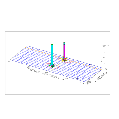
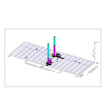
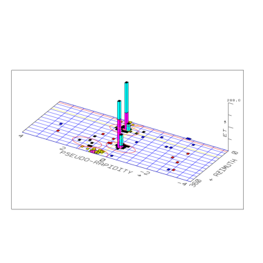
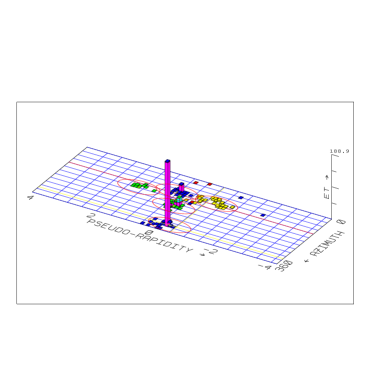
FIG. 1.: Jet events in the CDF calorimeter. A jet clustering cone of radius 0.7 is shown around each jet. Clockwise from the upper left they are identified as two-jet, two-jet, five-jet and three-jet. Tracks for these events are shown in Figure 2.

         

         

FIG. 2.: The same jet events in the CDF central tracking chamber. Clockwise from the upper left they are identified as two-jet, two-jet, five-jet and three-jet The calorimeter information for these events is shown in Figure 1.

FIG. 3.: Contributions of the various subprocesses to the inclusive jet cross section. This plot was generated with CTEQ4Mand $\mu=E_{T}/2$.

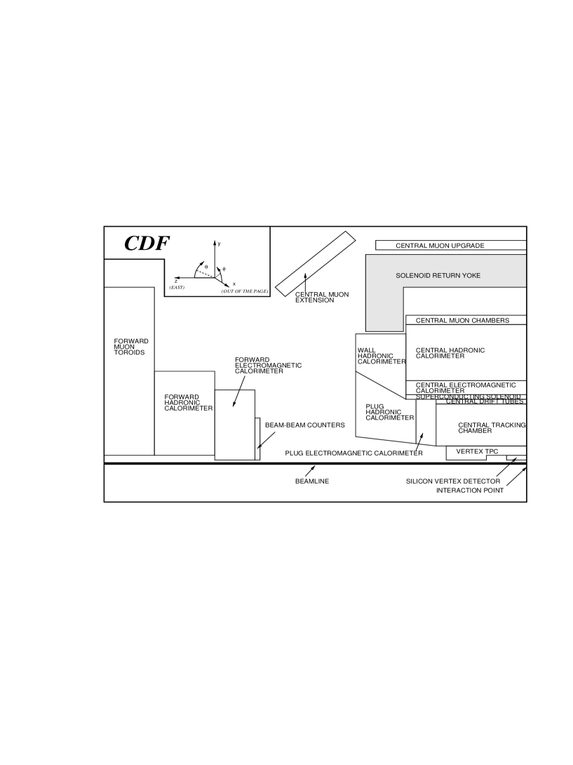
FIG. 4.: One quarter section of the CDF detector.

FIG. 5.: Minimum separation (in units of cluster radius) between the 3rd jet and the 1st or 2nd jet in different bins of jet $E_{T}$. At a separation of 1.3R at least 50% of the clusters are separated.

FIG. 6.: Trigger efficiency for the 100, 70, 50, and 20 GeV L2 triggers. The 100, 70, and 50 GeV triggers use overlap with the next lower trigger to determine the efficiency. The jet-20 plot uses the $2^{nd}$ jet in the event.

FIG. 7.: Percentage uncorrelated uncertainty on the Run 1A and 1B data sets.

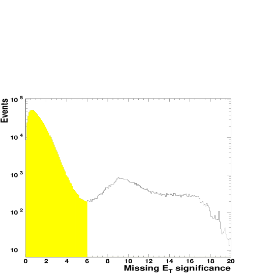
FIG. 8.: Distribution in $\tilde{\not\!\!E_{T}}$ after timing cut. The shaded region shows the events kept by the $\tilde{\not\!\!E_{T}}$ cut.

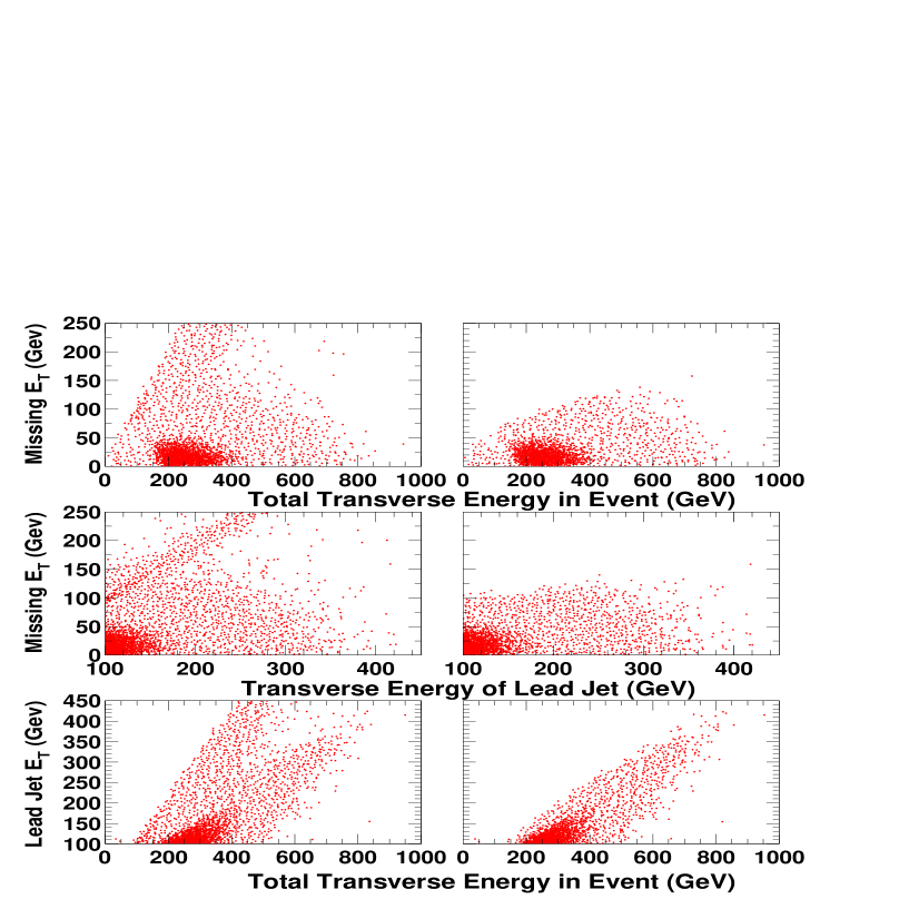
FIG. 9.: Raw data distributions before(left) and after(right) $\tilde{\not\!\!E_{T}}$ cut.

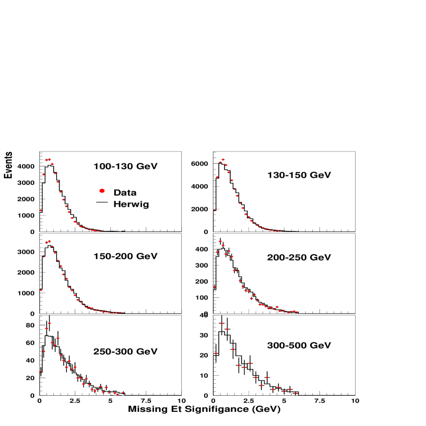
FIG. 10.: Distributions of missing $E_{T}$ significance from data (points) and HERWIG (histogram). The labels on the individual plots (e.g. 100-130 GeV) indicate the $E_{T}$ range of the leading jet.

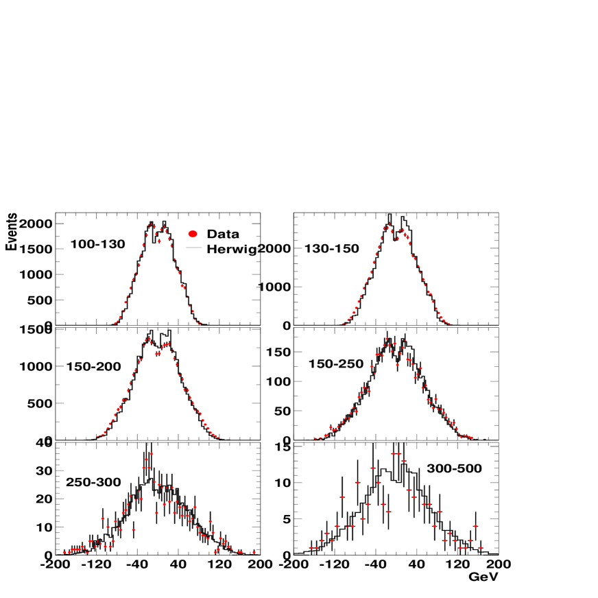
FIG. 11.: $E_{T}$ difference between leading two jets for data (points) and HERWIG (histogram). The sign of the difference is chosen based on sign($\phi_{1}-\phi_{2}$). The labels on the individual plots (e.g. 100-130 GeV) indicate the $E_{T}$ range of the leading jet.

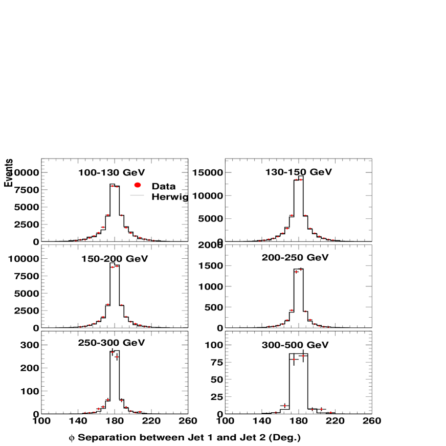
FIG. 12.: Difference in $\phi$ between leading two jets for data (points) and simulation (histogram). The labels on the individual plots (e.g. 100-130 GeV) indicate the $E_{T}$ range of the leading jet.

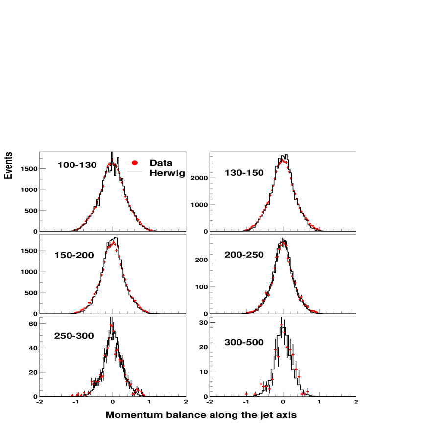
FIG. 13.: Fractional $E_{T}$ imbalance along dijet axis ($k_{||}$) for data (points) and simulation (histogram). The labels on the individual plots (e.g. 100-130 GeV) indicate the $E_{T}$ range of the leading jet.

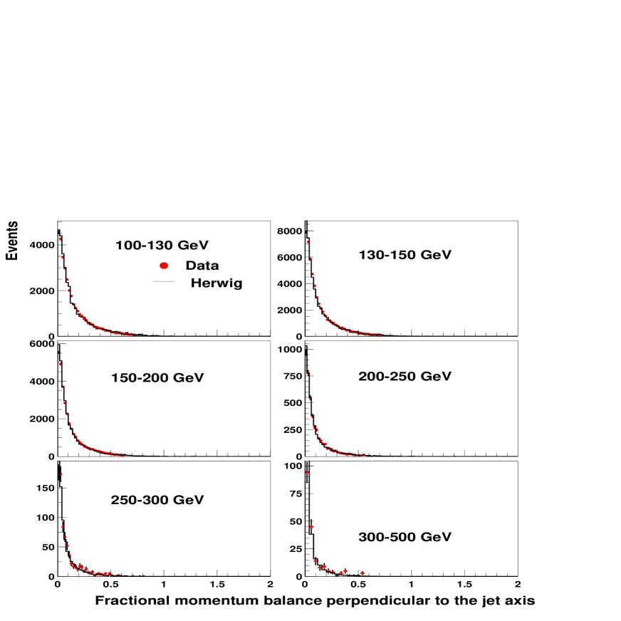
FIG. 14.: Fraction $E_{T}$ imbalance perpendicular to dijet axis ($k_{\perp}$) for data (points) and simulation (histogram). The labels on the individual plots (e.g. 100-130 GeV) indicate the $E_{T}$ range of the leading jet.

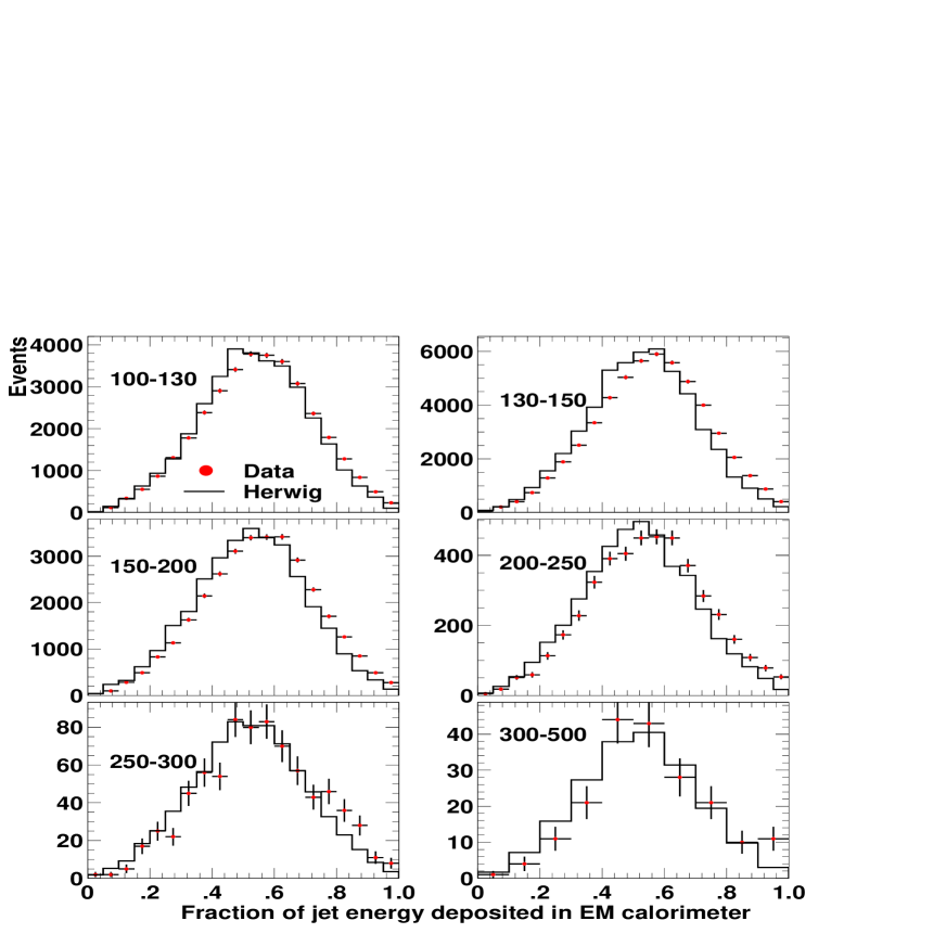
FIG. 15.: Fraction of electromagnetic energy in jets for data (points) and simulation (histogram). The labels on the individual plots (e.g. 100-130 GeV) indicate the $E_{T}$ range of the leading jet.

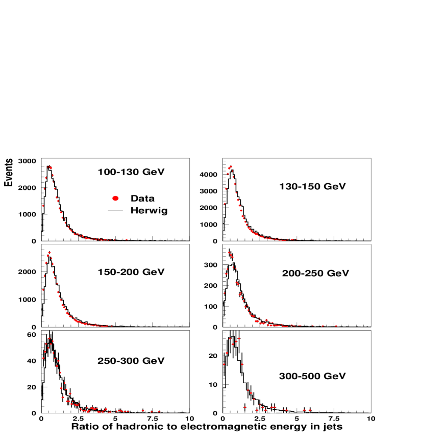
FIG. 16.: Ratio of hadronic to electromagnetic energy in jets for data (points) and simulation (histogram). The labels on the individual plots (e.g. 100-130 GeV) indicate the $E_{T}$ range of the leading jet.

FIG. 17.: In situ and test beam single particle response as a function of particle momentum. The stars indicate the response in the detector simulation.

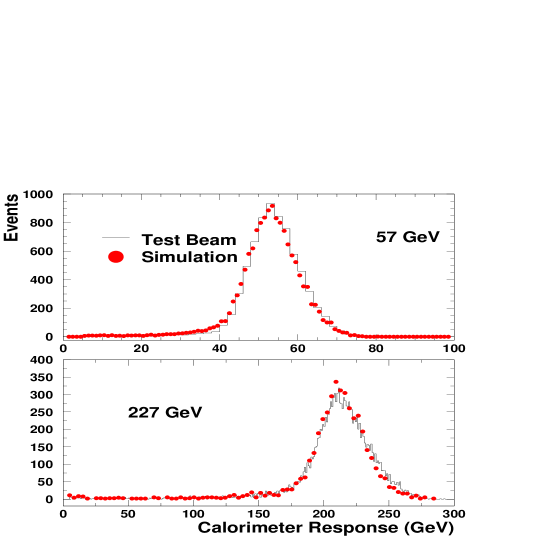
FIG. 18.: $E_{cal}/P_{\pi}$ for test beam pions and detector simulation.

FIG. 19.: The jet fragmentation properties for different $E_{T}$ jets using CDF-FF and HERWIG fragmentation functions

FIG. 20.: Fraction of jet energy in particles of different $P_{T}$

FIG. 21.: The fraction of jet $E_{T}$ carried by the (true) particles with $P_{T}<P_{T_{0}}$ using HERWIG

FIG. 22.: CDF calorimeter response for different $E_{T}^{True}$ jets

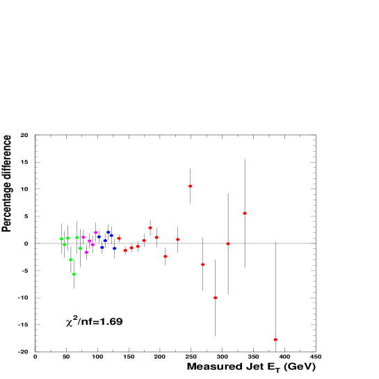
FIG. 23.: Residuals of the best fit curve (standard curve) and the measured cross section

FIG. 24.: Residuals of the best fit curve (standard curve) and the measured cross section. Distribution is fit to a Gaussian of width 1.0

FIG. 25.: The ratio of corrected $E_{t}$ and corrected cross section to the measured $E_{T}$ and measured cross section

FIG. 26.: Percentage difference between the corrected inclusive cross section data and the standard curve which was determined in the unsmearing process (see text) and represents the best smooth fit to the data.

FIG. 27.: Histogram of the residuals, (Data-curve)/error, of the corrected data compared to the standard curve. The curve is the result of a fit to a Gaussian of width 1.

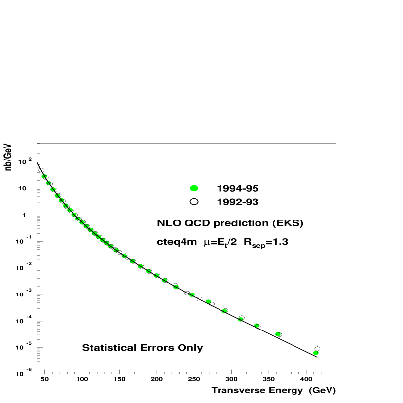
FIG. 28.: Inclusive jet cross section from the Run 1B data (94-95) compared to a QCD prediction and to the published Run 1A data (92-93).

FIG. 29.: The $\pm 1\sigma$ fractional change in cross section due to the dominate sources of systematic uncertainty.

FIG. 30.: Run 1B data compared to Run 1A smooth curve before (open) and after (solid) fitted shifts due to underlying event, energy scale stability and relative normalization have been included. Only the statistical uncertainty on the 1B data is shown.

FIG. 31.: Comparisons of D0 and CDF data to D0 smooth curve in the region 0.1$<|\eta|<$0.7.

FIG. 32.: The variation of the inclusive jet cross section for different $R_{sep}$ parameters. These calculations used the EKS program.

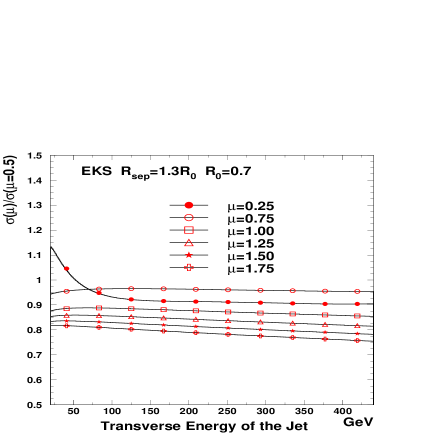
FIG. 33.: Variation in theory predictions for different renormalization scales.

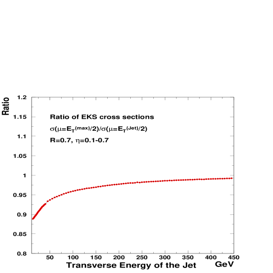
FIG. 34.: Comparison of NLO cross sections using $\mu=E_{t}^{max}/2$ and $\mu=E_{t}^{jet}/2$. The EKS program is used, $R_{sep}$ = 2.0, and the PDF’s are CTEQ3M.

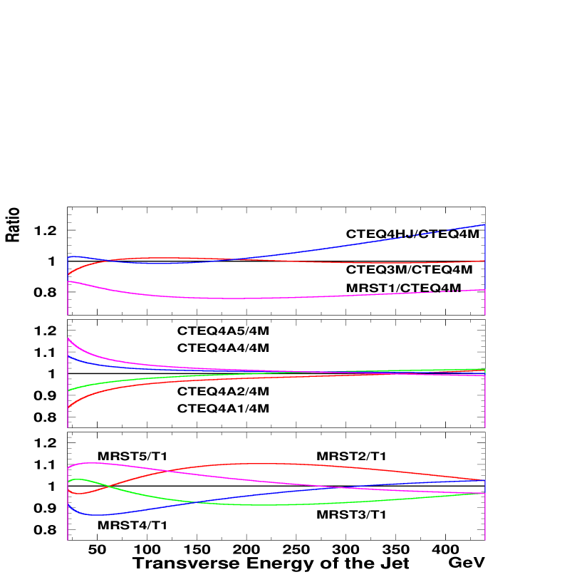
FIG. 35.: Variation in theory predictions for different parton distribution functions. In the top two plots the predictions have been normalized by CTEQ4M. In the bottom plot the different predictions have been divided by MRST.

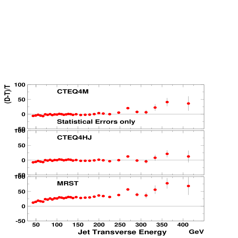
FIG. 36.: Run 1B data compared to QCD predictions (EKS, $\mu$=$E_{T}$/2, $R_{sep}$=1.3) using the CTEQ4M, CTEQ4HJ and MRST PDF’s. Only statistical uncertainties are shown on the data points.

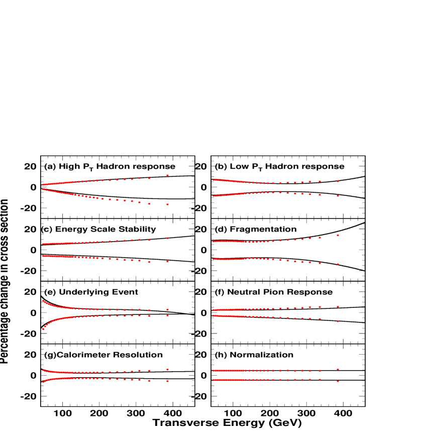
FIG. 37.: The fractional uncertainty on the raw CDF cross section (points) compared to the fractional uncertainty on the corrected CDF cross section (curves). The uncertainty on the corrected cross section is affected by the statistical precision on CDF data and hence the curves are not stable at very high $E_{T}$.

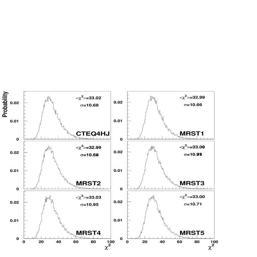
FIG. 38.: The $\chi^{2}$ distributions for pseudo-experiments using a variety of QCD predictions. For each plot, the pseudo-experiments are generated and fit to QCD predictions using the same PDF’s, e.g. for the upper left plot CTEQ4HJ is used to generate the data samples and the samples are fit to the nominal smeared CTEQ4HJ prediction.

FIG. 39.: The $\chi^{2}$ distributions for pseudo-experiments using a variety of QCD predictions. For each plot, the pseudo-experiments are generated and fit to QCD predictions using the same PDF’s e.g. for the upper left plot CTEQ4A1 is used to generate the data samples and the samples are fit to the nominal smeared CTEQ4A1 prediction

FIG. 40.: The $\Delta\chi^{2}$ distributions for CTEQ4HJ compared to the CDF standard curve, and theoretical predictions with the MRST series as described in the text. The arrows indicate the $\Delta\chi^{2}$ of the CDF data.

FIG. 41.: The $\Delta\chi^{2}$ distributions for CTEQ4HJ and theoretical predictions with the CTEQ4M series as described in the text. The arrows indicate the $\Delta\chi^{2}$ of the CDF data.

FIG. 42.: Matrix of correlation coefficients as defined in the text. Note the suppressed zero.

FIG. 43.: Matrix of correlation coefficients for infinite statistics as defined in the text.

FIG. 44.: Covariance matrix $\chi^{2}$ as a function of theory normalization factor for predictions with different PDF’s.

FIG. 45.: Data compared to theory before (open) and after (solid) shifts for four theoretical predictions.

FIG. 46.: Sequential sum of the fitted shifts.

TABLE I.: Coverage the CDF calorimeter components.

Central
Name	Rapidity	$\phi$-$\eta$ Segmentation
CEM	0.0- 1.1
CHA	0.0- 0.9	$15^{0}\times 0.1$
WHA	0.7 - 1.3
Forward
Name	Rapidity	$\phi$-$\eta$ Segmentation
PEM	1.1-2.4
PHA	1.3-2.4	$5^{0}\times 0.1$
FEM	2.2-4.2
FHA	2.3-4.2

TABLE II.: Trigger requirements for Run 1B jet data

Offline $E_{T}$ (GeV)	L2 $E_{T}$ (GeV)	L3 $E_{T}$ (GeV)	PS	Efficiency
40-45				96.3 $\pm$ 2%
45-50				98.5 $\pm$ 1%
50-55				99.3 $\pm$ 1%
55-60	Single Jet $>$ 20	Single Jet $>$ 10	967	99.7 $\pm$ 0.5%
60-65				99.9 $\pm$ 0.1%
65-70				100.0
70-75				100.0
75-80				94.7 $\pm$ 0.8%
80-85				98.0 $\pm$ 0.6%
85-90	Single Jet $>$ 50	Single Jet $>$35	39.5	94.7 $\pm$ 0.6%
90-95				94.7 $\pm$ 0.6%
95-100				94.7 $\pm$ 0.7 %
100-105				96.7 $\pm$ 0.3%
105-110				98.3 $\pm$ 0.3%
110-115	Single Jet $>$ 70	Single Jet $>$55	8.11	98.9 $\pm$ 0.3%
115-120				99.0 $\pm$ 0.3%
120-125				99.3 $\pm$ 0.3%
125-130				99.5 $\pm$ 0.3%
130-440	Sum Jet $>$ 175	Single Jet $>$80	1	$100^{+0.0}_{-0.5}\%$

TABLE III.: Bins in leading jet $E_{T}$ for comparison of event parameters to HERWIG + detector simulation

$E_{T}$ (GeV)	Trigger name
100-130	jet-70
130-150
150-200
200-250	jet-100
250-300
300-500

TABLE IV.: Underlying Event Energy: Raw $E_{T}$ in a cone of R = 0.7 in minimum bias data as a function of the number of found vertices

Vertices	$E_{T}$ in Cone(GeV)
0	0.48
1	1.27
2	2.18
3	3.01
4	3.78
$>$4	4.98

TABLE V.: CDF inclusive jet cross section and uncorrelated uncertainty from Run 1B data

Bin	$E_{T}$ (GeV)	cross section (nb/GeV)
1	$43.3$	$(0.576\pm 0.016)\times 10^{+2}$
2	$49.3$	$(0.290\pm 0.007)\times 10^{+2}$
3	$55.2$	$(0.160\pm 0.004)\times 10^{+2}$
4	$61.0$	$(0.893\pm 0.021)\times 10^{+1}$
5	$66.7$	$(0.528\pm 0.014)\times 10^{+1}$
6	$72.3$	$(0.355\pm 0.011)\times 10^{+1}$
7	$77.9$	$(0.226\pm 0.008)\times 10^{+1}$
8	$83.5$	$(0.154\pm 0.002)\times 10^{+1}$
9	$89.0$	$(0.102\pm 0.001)\times 10^{+1}$
10	$94.5$	$(0.729\pm 0.010)\times 10^{+0}$
11	$100.0$	$(0.513\pm 0.008)\times 10^{+0}$
12	$105.5$	$(0.378\pm 0.007)\times 10^{+0}$
13	$110.9$	$(0.274\pm 0.003)\times 10^{+0}$
14	$116.3$	$(0.199\pm 0.002)\times 10^{+0}$
15	$121.7$	$(0.151\pm 0.002)\times 10^{+0}$
16	$127.1$	$(0.116\pm 0.002)\times 10^{+0}$
17	$132.5$	$(0.877\pm 0.014)\times 10^{-1}$
18	$137.9$	$(0.659\pm 0.012)\times 10^{-1}$
19	$145.7$	$(0.466\pm 0.003)\times 10^{-1}$
20	$156.4$	$(0.281\pm 0.002)\times 10^{-1}$
21	$167.2$	$(0.178\pm 0.001)\times 10^{-1}$
22	$177.9$	$(0.115\pm 0.001)\times 10^{-1}$
23	$188.7$	$(0.763\pm 0.009)\times 10^{-2}$
24	$199.5$	$(0.520\pm 0.008)\times 10^{-2}$
25	$210.2$	$(0.344\pm 0.006)\times 10^{-2}$
26	$225.4$	$(0.195\pm 0.003)\times 10^{-2}$
27	$247.1$	$(0.968\pm 0.023)\times 10^{-3}$
28	$268.8$	$(0.535\pm 0.017)\times 10^{-3}$
29	$290.5$	$(0.236\pm 0.012)\times 10^{-3}$
30	$312.1$	$(0.117\pm 0.008)\times 10^{-3}$
31	$333.6$	$(0.685\pm 0.064)\times 10^{-4}$
32	$362.2$	$(0.322\pm 0.032)\times 10^{-4}$
33	$412.9$	$(0.630\pm 0.113)\times 10^{-5}$

TABLE VI.: Parameters for systematic error curves described in Equation 12 and shown in Figure 29.

	($P_{0}$)$\times 10^{+07}$	$P_{1}$	$P_{2}$	$P_{3}$	$P_{4}$	$P_{5}$	$P_{6}$
Standard Curve	0.14946	-2.9228	4.4881	-4.9447	1.7891	-0.2297	5.6147
Positive Systematic Uncertainties
High Pt Hadron	0.11521	-2.7511	4.4129	-4.9487	1.7989	-0.2325	5.3079
Low Pt hadron	0.16445	-2.9824	4.4867	-4.9415	1.7911	-0.2287	6.3165
Stability	0.15275	-2.9176	4.4883	-4.9449	1.7889	-0.2297	5.4732
Fragmentation	0.17922	-3.0070	4.4857	-4.9406	1.7917	-0.2285	6.5970
Und. Event	0.02392	-2.2945	4.4609	-4.9923	1.7764	-0.2228	5.8629
Neutral Pion	0.14852	-2.9146	4.4884	-4.9451	1.7888	-0.2298	5.4920
Resolution	0.10392	-2.8451	4.4958	-4.9455	1.7878	-0.2304	5.4340
Negative Systematic Uncertainties
High Pt Pion	0.12506	-2.7639	4.3972	-4.9442	1.8030	-0.2324	5.6243
Low Pt Pion	0.13604	-2.8651	4.4891	-4.9479	1.7870	-0.2306	4.9412
Stability	0.14757	-2.9299	4.4878	-4.9444	1.7892	-0.2296	5.7798
Fragmentation	0.12561	-2.8404	4.4904	-4.9487	1.7865	-0.2308	4.6655
Und. Event	0.34976	-3.1079	4.4710	-4.9422	1.7923	-0.2279	6.3048
Neutral Pion	0.15065	-2.9332	4.4877	-4.9443	1.7893	-0.2296	5.7700
Resolution	0.20458	-2.9888	4.4814	-4.9441	1.7901	-0.2291	5.7412

TABLE VII.: Estimates of theoretical uncertainty for three values of jet $E_{T}$. The % difference between various predictions is shown in Figures 32 to 35.

Source	% difference			Shape
	50 GeV	150 GeV	400 GeV
Clustering ($R_{sep}=2.0)$	5.2	4.8	4.0	Monotonic
Scale: $E_{T}^{jet}$ vs. $E_{T}^{max}$	6.0	3.0	1.0	Monotonic
Scale:$\mu=C*E_{T}^{jet}$, C=0.5 - 2.0	20	20	20	Flat
PDFs
CTEQ4 series (CTEQ4M ref.)	10	3	2	Monotonic
CTEQ4HJ (CTEQ4M ref.)	1	1	20	Not monotonic
MRST series (MRST ref.)	15	20	6	Not monotonic
MRST vs CTEQ4M	15	30	20	Not monotonic

TABLE VIII.: Results of the fit described by Equation 19. $\chi^{2}_{stat}$ represents the scatter of the points around a smooth curve, while the $\chi^{2}_{sys}$ represents the $\chi^{2}$ penalty from the systematic uncertainties. $\chi^{2}_{tot}$ is the sum of the two terms. The systematic shift columns show the individual $s_{k}$ for each systematic as defined in the text.

. PDF $\chi^{2}_{tot}$ $\chi^{2}_{stat}$ $\chi^{2}_{sys}$ Hi-Pi Lo-Pi Sta. Frg. UE $\pi^{0}$ Res. Norm. CDFSTD 42.3 41.3 1.0 -0.380 -0.223 -0.285 0.791 -0.141 -0.140 0.056 -0.278 CTEQ4M 63.4 48.2 15.2 -0.395 -0.411 -0.500 2.350 -1.443 0.168 0.937 -2.467 CTEQ4HJ 46.8 40.7 6.1 0.329 -0.741 -0.549 1.686 -1.235 -0.166 -0.053 -0.872 CTEQ4A1 60.1 47.1 13.0 -0.001 -0.670 -0.560 2.401 -0.877 0.075 0.875 -2.219 CTEQ4A2 61.5 47.4 14.1 -0.083 -0.667 -0.604 2.404 -1.126 0.073 0.833 -2.358 CTEQ4A3 63.4 48.2 15.2 -0.395 -0.411 -0.500 2.350 -1.443 0.168 0.937 -2.467 CTEQ4A4 64.5 48.8 15.7 -0.365 0.061 -0.732 2.270 -1.555 0.026 0.866 -2.597 CTEQ4A5 67.0 49.8 17.2 -0.490 0.214 -0.751 2.264 -1.723 -0.068 0.911 -2.719 MRST 49.5 40.8 8.7 0.743 0.756 0.684 2.123 -1.508 0.485 -0.293 0.210 MRST-g$\uparrow$ 53.3 43.3 10.0 0.773 -0.314 0.166 2.677 -1.014 0.283 0.030 -1.005 MRST-g$\downarrow$ 59.2 45.7 13.5 0.687 1.726 1.166 1.741 -1.879 0.699 -0.692 1.068 MRST-$\alpha_{s}\downarrow\downarrow$ 59.7 41.4 18.3 2.436 -0.050 0.581 2.604 -1.302 0.362 -1.234 1.391 MRST-$\alpha_{s}\uparrow\uparrow$ 53.4 43.9 9.5 -0.221 1.413 0.508 1.922 -1.640 0.440 0.309 -0.731

TABLE IX.: The effect of including limited systematic uncertainties in the fit to QCD predictions using CTEQ4HJ PDF’s. The first column indicates the number of systematic uncertainties included (e.g. the first row is with no systematic uncertainties). The next three columns indicate the total $\chi^{2}$, the contribution from the uncorrelated scatter of the points around a smooth curve, $\chi^{2}_{stat}$, and the penalty from the correlated shifts from the systematics uncertainties $\chi^{2}_{sys}$ . The remaining eight columns represent the $s_{k}$ which result from the fit for the eight systematic uncertainties as described in the text.

	$\chi^{2}_{total}$	$\chi^{2}_{stat}$	$\chi^{2}_{sys}$	Hi-Pi	Lo-Pi	Stab.	Frg	UE	$\pi^{0}$	Res.	Norm.
0	94.2	94.2	0.00	0.000	0.000	0.000	0.000	0.000	0.000	0.000	0.000
1	79.0	79.0	0.0	0.000	0.000	0.000	0.000	-0.200	0.000	0.000	0.000
2	62.9	59.5	3.4	0.000	0.000	0.000	0.500	0.000	0.000	-1.787	0.000
3	49.1	43.3	5.8	0.000	-1.459	0.000	1.412	-1.304	0.000	0.000	0.000
4	47.6	40.7	6.9	0.000	-1.301	0.000	1.729	-1.255	0.000	0.000	-0.821
5	47.1	40.4	6.7	0.000	-0.950	-0.583	1.883	-1.213	0.000	0.000	-0.686
6	46.9	40.7	6.2	0.339	-0.782	-0.585	1.664	-1.259	0.000	0.000	-0.868
7	46.9	40.7	6.2	0.338	-0.749	-0.557	1.682	-1.261	-0.169	0.000	-0.860
8	46.9	40.7	6.2	0.329	-0.741	-0.549	1.686	-1.234	-0.166	-0.053	-0.871

TABLE X.: As in previous table except the QCD predictions use MRST PDF’s.

	$\chi^{2}_{total}$	$\chi^{2}_{stat}$	$\chi^{2}_{sys}$	Hi-Pi	Lo-Pi	Stab.	Frg	UE	$\pi^{0}$	Res.	Norm.
0	11039.8	11039.8	0.00	0.000	0.000	0.000	0.000	0.000	0.000	0.000	0.000
1	141.1	124.4	16.7	0.000	0.000	4.083	0.000	0.000	0.000	0.000	0.000
2	73.2	48.0	25.2	0.000	0.000	0.000	4.486	-2.259	0.000	0.000	0.000
3	53.4	39.8	13.6	0.000	0.931	0.000	3.270	-1.433	0.000	0.000	0.000
4	50.8	40.2	10.6	1.065	1.151	0.000	2.382	-1.584	0.000	0.000	0.000
5	50.0	40.4	9.6	0.887	0.827	0.780	2.194	-1.657	0.000	0.000	0.000
6	49.8	40.5	9.3	0.840	0.735	0.711	2.134	-1.656	0.499	0.000	0.000
7	49.6	40.7	8.9	0.800	0.771	0.723	2.140	-1.496	0.502	-0.322	0.000
8	49.5	40.8	8.7	0.743	0.756	0.684	2.123	-1.508	0.485	-0.293	0.210

TABLE XI.: Comparison of CDF Run 1B data to various theoretical predictions using the $\chi^{2}$ and the $\Delta\chi^{2}$ statistics.

PDF	$\chi^{2}$	$CL(\%)$	$\chi^{2}-\chi^{2}_{cteq4hj}$	Prob. Rel. to CTEQ4HJ
CDFSTD	42.3	16	-4.5	10
CTEQ4HJ	46.8	10	0.0	1
MRST	49.6	7.4	2.7	0.5
MRST-g$\uparrow$	53.3	4.6	6.5	0.06
MRST-g$\downarrow$	59.2	2.4	12.4	0.01
MRST-$\alpha_{s}\downarrow\downarrow$	59.8	2.0	12.9	$<10^{-4}$
MRST-$\alpha_{s}\uparrow\uparrow$	53.4	4.8	6.6	0.07
CTEQ4A1	60.1	2.1	13.3	$<10^{-4}$
CTEQ4A2	61.6	1.8	14.7	$<10^{-4}$
CTEQ4M	63.4	1.4	16.6	$10^{-3}$
CTEQ4A4	64.5	1.3	17.7	$10^{-3}$
CTEQ4A5	67.0	1.0	20.2	$<10^{-4}$

TABLE XII.: Covariance matrix $\chi^{2}$ comparison for various theoretical predictions for Run 1B jet data. The $\chi^{2}$ for the nominal curve is 46.3 for 33 bins with only statistical uncertainty and when the systematics uncertainty is included.

PDF	Stat. only	Stat. and Sys.
CTEQ3M	227.0	81.2
CTEQ4M	119.9	70.0
CTEQ4HJ	85.4	52.2
MRST-g$\downarrow$	12204.0	56.0
MRST-g$\uparrow$	4363.0	54.6

TABLE XIII.: Minimum value of the covariance matrix $\chi^{2}$ and corresponding theory normalization factor.

	Sys. unc. OFF		Sys. unc. ON
PDF	$\chi^{2}$	Norm.	$\chi^{2}$	Norm.
CTEQ3M	118.9	0.97	51.7	0.68
CTEQ4M	101.6	0.99	51.3	0.74
CTEQ4HJ	75.3	0.99	49.6	0.88
MRST-g$\downarrow$	569.0	1.38	51.3	1.22
MRST-g$\uparrow$	90.8	1.19	52.2	0.88

TABLE XIV.: Covariance matrix $\chi^{2}$ comparison for various theoretical predictions for 1B jet data where only the indicated systematic uncertainties is included.

Sys. Uncertainty	MRST-g$\downarrow$ $\chi^{2}$	CTEQ4HJ $\chi^{2}$
Hi-Pi	248.6	77.2
Low-Pi	1330.0	75.2
Stability	127.9	76.1
Fragmentation	382.1	75.9
UE	3630.0	69.6
Neutral Pi	179.5	76.2
Resolution	1952.0	71.0
Normalization	359.6	75.2

TABLE XV.: Results of fits to various PDF’s. The first line shows the $\chi^{2}$ when only the uncorrelated errors on the data points are included. The next two rows show the contribution to the total $\chi^{2}$ from the data - theory term and the $\sum{S_{K}}$ term.

PDF	CDFSTD	CTEQ3M	CTEQ4M	CTEQ4HJ	MRST	MRST-g$\uparrow$	MRST-g$\downarrow$
stat.only	44.16	220.0	116.5	83.5	8119.3	4394.9	12271.5
1st term	43.66	67.75	60.52	46.33	42.70	48.05	43.13
$\sum{S_{K}}$	1.63e-2	14.07	9.74	4.33	4.90	6.87	9.52
total	43.68	81.82	70.27	50.57	47.61	54.92	52.64

TABLE XVI.: Individual fit parameters for fit results in Table XV

PDF	STD	CTEQ3M	CTEQ4M	CTEQ4HJ	MRST	MRST-g$\uparrow$	MRST-g$\downarrow$
Hi-Pi	0.0057	4.23e-7	0.0020	0.710	-0.478	0.0078	-1.13
Lo-Pi	-0.0048	0.861	0.159	-0.702	-0.937	-0.722	-1.35
Stab.	0.0023	-0.0086	-6.2e-6	0.288	-0.629	-0.227	-0.741
Frag.	-0.0053	-1.365	-1.44	-1.192	-1.433	-2.046	-0.879
UE	0.0086	0.5998	0.926	1.119	0.950	0.695	1.121
Neutral Pi	3.34e-3	-0.245	-0.0049	1.3e-4	-0.534	-0.279	-0.559
Res.	3.83e-3	-1.878	-1.235	0.0071	0.180	-0.752	1.131
Norm.	1.63e-4	2.74	2.29	0.761	-0.354	0.987	-1.494

TABLE XVII.: Results of fits to various PDF’s with normalization as a free parameter. The first line shows the $\chi^{2}$ when only the uncorrelated errors on the data points are included. The next two rows show the contribution to the total $\chi^{2}$ from the data - theory term and the $\sum{S_{K}}$ term.

PDF	STD	CTEQ3M	CTEQ4M	CTEQ4HJ	MRST	MRST-g$\uparrow$	MRST-g$\downarrow$
stat.only	43.8	113.0	99.9	74.1	216.0	86.5	575.0
1st term	43.66	46.63	45.76	43.90	43.01	45.16	42.88
$\sum{S_{K}}$	1.63e-2	9.59	8.11	4.81	4.26	7.19	4.08
total	43.68	56.22	53.88	48.71	47.27	52.35	46.96

TABLE XVIII.: Individual fit parameters for fit results in Table XVII. Normalization is a free parameter.

PDF	STD	CTEQ3M	CTEQ4M	CTEQ4HJ	MRST	MRST-g$\uparrow$	MRST-g$\downarrow$
Hi-Pi	0.057	-0.813	-0.398	0.444	-0.346	-0.846e-4	-0.586
Lo-Pi	-0.048	0.863	-1.068	-1.23	-0.689	-1.21	-0.329
Stab.	0.023	-1.114	-0.882	-0.054	-0.555	-0.662	-0.449
Frag.	-0.053	-2.247	-2.205	-1.405	-1.434	-2.10	-0.943
UE	0.086	0.070	0.537	0.997	1.026	0.576	1.441
Neutral Pi	.327e-2	-0.947	-0.764	-0.081	-0.493	-0.579	-0.411
Res.	.392e-2	-0.997	-0.554	0.341	0.041	-0.477	0.540
Norm	.842e-3	9.22	7.363	2.57	-.964	2.53	-3.86

TABLE XIX.: The effect of including limited systematic uncertainties in the fit to QCD predictions using MRST-g$\downarrow$ PDF’s. The first column indicates the number of systematic uncertainties included (e.g. the first row is with no systematic uncertainties). The next three columns indicate the total $\chi^{2}$, the contribution from the uncorrelated scatter of the points around a smooth curve, $\chi^{2}_{stat}$, and the penalty from the correlated shifts from the systematics uncertainties, $\chi^{2}_{sys}$. The remaining eight columns represent the results of the fit (the $s_{k}$) eight systematic uncertainties as described in the text.

	$\chi^{2}_{total}$	$\chi^{2}_{stat}$	$\chi^{2}_{sys}$	Hi-Pi	Lo-Pi	Stab.	Frg	UE	$\pi^{0}$	Res.	Norm.
0	18044.1	18044.1	0.0	0.000	0.000	0.000	0.000	0.000	0.000	0.000	0.000
1	268.0	242.9	25.1	0.000	5.010	0.000	0.000	0.000	0.000	0.000	0.000
2	103.7	52.5	51.2	0.000	0.000	6.784	0.000	-2.282	0.000	0.000	0.000
3	69.2	49.0	20.2	0.000	2.178	0.000	3.449	-1.884	0.000	0.000	0.000
4	64.2	45.4	18.7	0.000	2.000	0.000	2.729	-1.988	0.000	0.000	1.809
5	61.5	45.4	16.1	0.000	1.515	1.393	2.265	-2.143	0.000	0.000	1.473
6	60.4	45.6	14.8	0.789	1.770	1.208	1.806	-2.216	0.000	0.000	1.186
7	59.7	45.6	14.1	0.740	1.850	1.252	1.822	-1.884	0.000	-0.681	1.116
8	59.2	45.7	13.5	0.686	1.726	1.166	1.741	-1.879	0.699	-0.692	1.069

TABLE XX.: As in previous table except with CTEQ4M PDF’s.

	$\chi^{2}_{total}$	$\chi^{2}_{stat}$	$\chi^{2}_{sys}$	Hi-Pi	Lo-Pi	Stab.	Frg	UE	$\pi^{0}$	Res.	Norm.
0	138.5	138.5	0.00	0.000	0.000	0.000	0.000	0.000	0.000	0.000	0.000
1	110.9	110.8	0.1	0.000	0.000	0.000	0.000	-0.269	0.000	0.000	0.000
2	90.4	89.6	0.8	0.000	0.000	0.000	0.336	-0.812	0.000	0.000	0.000
3	66.9	52.6	14.3	0.000	0.000	0.000	1.969	-0.841	0.000	0.000	-3.116
4	65.1	50.6	14.5	0.000	0.000	0.000	1.876	-1.159	0.000	0.603	-3.043
5	63.97	48.7	15.2	0.000	0.000	-0.655	2.182	-1.483	0.000	0.974	-2.622
6	63.7	48.7	15.0	-0.255	0.000	-0.730	2.315	-1.350	0.000	0.870	-2.551
7	63.5	48.3	15.2	-0.399	-0.372	-0.465	2.376	-1.451	0.000	0.945	-2.456
8	63.4	48.2	15.2	-0.396	-0.412	-0.501	2.350	-1.443	0.168	0.937	-2.467

REFERENCES

- [1] F. Abe et al. (CDF Collaboration), Nucl. Instrum. Methods A271, 387 (1988); Nucl. Instrum. Methods A268,75 (1988) and references therein.
- [2] F. Abe et al. (CDF Collaboration), Phys. Rev. Lett. 77 438(1996).
- [3] F. Abe et al. (CDF Collaboration), Phys. Rev. Lett. 68 1104(1992).
- [4] F. Abe et al. (CDF Collaboration), Phys. Rev. Lett. 62 613(1989).
- [5] E. Eichten, K. Lane, and M. Peskin, Phys. Rev. Lett. 50, 811 (1983).
- [6] J. Huston et al., Phys. Rev. Lett. 77, 444(1996).
- [7] W. Giele and S. Keller Preprint hep-ph/9803393, FNAL-Pub-98/082-T.
- [8] J. Huston et al., Phys. Rev. Lett. 77, 444(1996).
- [9] F. Abe et al. (CDF Collaboration), Phys. Rev. D50 5550, (1994), D. Cronin-Hennessy et al. (CDF Collaboration), Nucl. Instrum. Methods A433 (2000) 37 and M. Albrow, et al. CDF NOTE 4844, FERMILAB-TM-2071 (1999).
- [10] B. Abbot et al. (D0 Collaboration), Phys.Rev.Lett. 82, 2451 (1999).
- [11] S.M. Berman, M. Jacob, Phys. Rev. Lett. 25 1683 (1970); S.M. Berman, J.D. Bjorken and J.B. Kogut, Phys. Rev. 4D 3388 (1971); R.P. Feynman: Photon hadron interactions. New York: Benjamin 1972.
- [12] M.G. Albrow et al., Nucl Phys. B160 1 (1979); A.L.S. Angelis et al., Phys Scr. 19 116 (1979); A.G. Clark et al., Nucl. Phys. B160 397 (1979); D. Drijard et al., Nucl. Phys. B166 233 (1980).
- [13] M. Banner et al. (UA2 Collaboration), Phys. Lett. 118B 203 (1982).
- [14] G. Arnison et al. (UA1 Collaboration), Phys. Lett. 123B 115 (1983).
- [15] T. Akesson et al. (AFS Collaboration), Phys. Lett. 118B 185 (1982) ; A.L.S. Angelis et al., Phys. Lett. 126B 132 (1983).
- [16] J.A. Appel et al. (UA2 Collaboration), Phys. Lett. 165B 441 (1985).
- [17] F. Abe et al. (CDF Collaboration), Phys. Rev. 44D 601 (1991).
- [18] R.K. Ellis, W.J.Stirling and B.R. Webber ”QCD and Collider Physics” Cambridge Monographs on Particle Physics, Nuclear Physics and Cosmology, Cambridge Univ. Press, United Kingdom (1996).
- [19] B.L. Combridge, J. Kripfganz and J. Ranft, Phys. Lett. 70B 234 (1977).
- [20] F. Aversa, P. Chiappetta, M. Greco, P. Guillet, Phys. Lett. B 210, 225 (1988); 211, 465 (1988); Nucl. Phys. B327, 105 (1989).
- [21] S. Ellis. Z. Kunszt, and D. Soper, Phys. Rev. Lett. 62 2188 (1989); Phys. Rev. Lett. 64 2121 (1990); Phys. Rev. D 40 2188 (1989).
- [22] S.K. Ellis, Z. Kunszt, D. Soper, Phys. Rev. Lett. 69 3615 (1992) and S. Ellis CERN–TH–6861–93 In proceedings of 28th Rencontres de Moriond: QCD and High Energy Hadronic Interactions, Les Arcs, France, 20-27 Mar 1993. hep-ph/9306280.
- [23] B. Flaugher and K. Meier “Proceedings 1990 Summer Study on High Energy Physics, ed. E Berger. Singapore: World Scientific, 128 (1992).
- [24] P. Bagnaia et al. (UA2 Collaboration), Z. Phys. C20 117 (1983).
- [25] G. Arnison et al. (UA1 Collaboration), Phys. Lett. 132B 214 (1983).
- [26] P. Bagnaia et al. (UA2 Collaboration), Phys. Lett. 138B 430 (1984).
- [27] F.E. Paige and S.D. Protopopescu, ISAJET, BNL 31987.
- [28] E. Eichten et al., Phys. Rev. Lett. 50 811 (1983). M. Abolins et al., Proc. DPF summer study on elementary particle physics, Snowmass, Co. 274 (1982).
- [29] G. Arnison et al. (UA1 Collaboration), Phys. Lett. 136B 294 (1984).
- [30] G. Arnison et al. (UA1 Collaboration), Phys. Lett. 177B 244 (1986) .
- [31] J.A. Appel et al. (UA2 Collaboration), Phys. Lett. 160B 349 (1985) .
- [32] P. Bagnaia et al. (UA2 Collaboration), Phys. Lett. 144B 283 (1984) .
- [33] P. Bagnaia et al. (UA2 Collaboration), Phys. Lett. 186B 452 (1987) .
- [34] G. Arnison et al. (UA1 Collaboration), Phys. Lett. 158B 494 (1985) .
- [35] G. Arnison et al. (UA1 Collaboration), Z. Phys. C36 33 (1987).
- [36] J.A. Appel et al. (UA2 Collaboration), Z. Phys. C30 341 (1986).
- [37] G. Arnison et al. (UA1 Collaboration), Phys. Lett. 172B 461 (1983).
- [38] G. Altarelli ”QCD at the Collider” Presented at Inst. School of Subnuclear Physics, Erice, Italy, Aug 3-14, 1983. CERN TH-3733 (1983).
- [39] H.U. Bengtsson and T. Sjostrand, PYTHIA, Comput. Phys. Commun. 46 43 (1987).
- [40] G. Marchesini and B. R. Webber, Nucl. Phys. B310, 461 (1988).
- [41] J. Alitti et al. (UA2 Collaboration), Phys. Lett. 257B 232 (1991).
- [42] T. Sjostrand and H.U. Bengtsson, JETSET, Comput. Phys. Commun. 43 (1987).
- [43] J. Huth et al. “Proceedings 1990 Summer Study on High Energy Physics, ed. E Berger. Singapore: World Scientific, 134 (1992).
- [44] Walter T. Giele (Fermilab). FERMILAB-CONF-97-240-T, Jul 1997, Proceedings of 5th International Workshop on Deep Inelastic Scattering and QCD (DIS 97), Chicago, IL, 14-18 Apr 1997, hep-ph/9707300; and W. T. Giele, E.W.N. Glover and J. Yu, FERMILAB-PUB-127-T, DTP/95/52. hep-ph/9506442 (1995).
- [45] W. T. Giele, E.W.N. Glover and D.A. Kosower, Nucl. Phys. B403 633 (1993).
- [46] F. Abe et al. (CDF Collaboration), Phys. Rev. Lett. 62 3020 (1989).
- [47] F. Abe et al. (CDF Collaboration), Phys. Rev. Lett. 64 157 (1990).
- [48] F. Abe et al. (CDF Collaboration), Phys. Rev. D41 1722 (1990).
- [49] F. Abe et al. (CDF Collaboration), Phys. Rev. Lett. 69 2896 (1992).
- [50] F. Abe et al. (CDF Collaboration), Phys. Rev. D48 998 (1993).
- [51] F. Abe et al. (CDF Collaboration), Phys. Rev. Lett. 71 2542 (1993).
- [52] F. Abe et al. (CDF Collaboration), Phys. Rev. Lett. 74 3538 (1995).
- [53] F. Abe et al. (CDF Collaboration), Phys. Rev. Lett. 77 5336 (1996).
- [54] F. Abe et al. (CDF Collaboration), Phys. Rev. D55 5263 (1997).
- [55] F. Abe et al. (CDF Collaboration), Phys. Rev. Lett. 70 1376 (1993) .
- [56] F. Abe et el. (CDF Collaboration), Phys. Rev. D45 1448 (1992).
- [57] F. Abe et al. (CDF Collaboration), Phys.Rev. D56 2532 (1997); Phys.Rev. D54 4221 (1996); Phys.Rev.Lett.75 608 (1995); Phys.Rev. 45 2249 (1992).
- [58] C. Haber et al. Nucl. Instrum. Methods A289 388 (1990).
- [59] F. Abe et el. (CDF Collaboration), Phys.Rev.D50 2966 (1994).
- [60] F. Abe et el. (CDF Collaboration), Phys.Rev. Lett. 65 968 (1990).
- [61] F. Abe et al. (CDF Collaboration), Phys.Rev. 59 052002 (1999).
- [62] F. Abe et al. (CDF Collaboration), Phys.Rev.Lett.84 485 (2000).
- [63] This uncertainty is not included in the inclusive jet cross section reported by the D0 collaboration.
- [64] F. Abe et el. (CDF Collaboration), Phys.Rev.D80 5720 (1998).
- [65] ’MINUIT’ A System for Function Minimization and Analysis of the Parameter Errors and Correlations. F. James, M. Roos Comput.Phys.Commun.10 343 (1975).
- [66] The D0 data is presented in [10]. The curve was provided by Private Communication with Bob Hirosky (D0 Collaboration).
- [67] G. Blazey and B. Flaugher ”Inclusive Jet and Dijet production at the Tevatron” to be published in Annu. Rev. Nucl. Part. Sci. 1999; FERMILAB-PUB-99/038-E, hep-ex/9903058.
- [68] Z.Kunszt and D.Soper, Phys. Rev. D46 192 (1992), and http://zebu.uoregon.edu/ soper/soper.html, program version 3.4.
- [69] M. Arneodo et al. (NMC Collaboration), Nucl. Phys. B483 3 (1997); M. Arneodo et al., Phys. Lett. B364, 107 (1995).
- [70] M.R. Adams et al. (E665 collaboration), Phys. Rev. D54 3006 (1996).
- [71] S. Aid et al. (H1 collaboration), Nucl. Phys. B470 3 (1996); C. Adloff et al., Nucl. Phys. B497 3 (1997); C. Adloff et al., Z. Phys. C72 593 (1996); S. Aid et al., Nucl. Phys. B439, 471 (1995).
- [72] M. Derrick et al. (ZEUS collaboration), Z. Phys. C69 (1996) 607; M. Derrick et al., Z. Phys. C72 399 (1996); J. Breitweg et al., Eur. Phys. J. C7, 609 (1999), hep-ex/9809005; J. Breitweg et al., Phys. Lett. B407 402 (1997); Paper N-645 presented at International Europhysics Conference on High Energy Physics, HEP97, Jerusalem 1997. M. Derrick et al., Z. Phys. C65, 379 (1995).
- [73] G. Moreno et al. (E605 collaboration), Phys. Rev. D43 2815 (1991)
- [74] E.A. Hawker et al. (E866 collaboration), Phys. Rev. Lett. 80 3715 (1998), hep-ex/9803011.
- [75] F. Abe et al. (CDF Collaboration), Phys. Rev. Lett. 74, 850 (1995); F. Abe et al. (CDF Collaboration), Phys. Rev. Lett., 81, 5754 (1998), hep-ex/9809001.
- [76] H. L. Lai et al., Phys. Rev. D 55, 1280 (1997).
- [77] A.D. Martin, R.G. Roberts, W.J. Stirling and T hep–ph/9803445, Eur. Phys. J. C C 4, 463 (1998)
- [78] C. Bromberg et al. (E706 Collaboration), Influence of Parton k(t) on High-p(t) Particle Production and Determination of the Gluon Distribution Function, In Proceedings of the 29th International Conference on High-Energy Physics (ICHEP 98), Vancouver, British Columbia, Canada, 23-29 Jul 1998. Vol. 1 867.
- [79] J. Huston et al., Phys.Rev. D58 114034 (1998), hep–ph/9801444.
- [80] U.K Yang, A. Bodek, Phys.Rev.Lett. 82 2467 (1999).
- [81] F. Abe et el. (CDF Collaboration), Phys.Rev.D80 2773 (1998).
- [82] Walter Giele, Next to leading order PQCD calculations, 10th Topical Workshop in proton-antiproton Collider Physics, Fermilab, (1995). FERMILAB-CONF-95-169-T.
- [83] E. Laenen, G. Oderda, G. Sterman Phys. Lett. B438 173 (1998).
- [84] F. Abe et al. (CDF Collaboration), Phys. Rev. D61:091101 (2000); F. Abe et al. (CDF Collaboration), in preparation.
- [85] W.H. Press, B.P. Flannery, S.A. Teukolsky, and W.T. Vetterling ”Numerical Recipies, The Art of Scientific Computing” Cambridge University Press (1986).
- [86] S. Cantani, M.L. Mangano, P. Nason, L. Trentadue Nucl. Phys. B478 273 (1996).
- [87] Louis Lyons ”Seleting between two hypotheses” OUNP-99-12.
- [88] G.D’Agostini ”Probaility and measurement Uncertainty in Physics - a Bayesain primer” hep/ph/9512295v2.