xxx

Flavour Dynamics: CP Violation and Rare Decays

Andrzej J. Buras

Technische Universität München

Physik Department

D-85748 Garching, Germany

Abstract

These lectures give an up to date description of CP violation and rare decays of K and B mesons and consist of ten chapters: i) Grand view of the field including CKM matrix and the unitarity triangle, ii) General aspects of the theoretical framework based on effective weak Hamiltonians, the operator product expansion and the renormalization group, iii) Particle-antiparticle mixing and various types of CP violation, iv) Standard analysis of the unitarity triangle, v) The ratio $\varepsilon^{\prime}/\varepsilon$, vi) Rare decays $K^{+}\to\pi^{+}\nu\bar{\nu}$ and $K_{L}\to\pi^{0}\nu\bar{\nu}$, vii) Express review of other rare decays, viii) CP violation in B decays, ix) A brief look beyond the Standard Model discussing in particular the models with minimal flavour violation, x) Perspectives for the coming years.

Lectures given at the 38th Course of

the Erice International School of Subnuclear Physics:

Theory and Experiment Heading for New Physics

27 August–5 September, 2000

Flavour Dynamics: CP Violation and Rare Decays

Andrzej J. Buras

Technische Universität München

Physik Department

D-85748 Garching, Germany

Contents:

1. Grand View, 2. Theoretical Framework, 3. Particle-Antiparticle Mixing and Various Types of CP Violation, 4. Standard Analysis of the Unitarity Triangle, 5. $\varepsilon^{\prime}/\varepsilon$ in the Standard Model, 6. The Decays $K^{+}\to\pi^{+}\nu\bar{\nu}$ and $K_{L}\to\pi^{0}\nu\bar{\nu}$, 7. Express Review of Rare K- and B-Decays, 8. CP Violation in B Decays, 9. Looking Beyond the Standard Model, 10. Perspectives.

1 Grand View

1.1 Preface

Flavour dynamics and the related origin of quarks and lepton masses and mixings are among the least understood topics in the elementary particle physics. While the definite understanding of flavour dynamics will most probably come from a fundamental theory at very short distance scales, as the GUT scale or the Planck scale, it is commonly accepted that the study of CP-violating and rare decay processes plays an important role in the search for this fundamental theory.

In this context an important issue is the question whether the Standard Model (SM) of fundamental interactions is capable of describing the violation of CP symmetry observed in nature. Actually this question has already been answered through the studies of a dynamical generation of the baryon asymmetry in the universe, which is necessary for our existence. It turns out that the size of CP violation in the SM is too small to generate a large enough matter-antimatter asymmetry observed in the universe today.

On the other hand it is conceivable that the physics responsible for the baryon asymmetry involves only very short distance scales, as the GUT scale or the Planck scale, and the related CP violation is unobservable in the experiments performed by humans. Yet even if such an unfortunate situation is a real possibility, it is unlikely that the SM provides an adequate description of CP violation at scales accessible to experiments peformed on our planet in this millennium. On the one hand the Kobayashi-Maskawa (KM) picture of CP violation is so economical that it is hard to believe that it will pass future experimental tests. On the other hand almost any extention of the SM contains additional sources of CP violating effects. As some kind of new physics is required in order to understand the patterns of quark and lepton masses and mixings and generally to understand the flavour dynamics, it is very likely that this physics will bring new sources of CP violation modifying KM picture considerably.

Similarly to CP violation, particle-antiparticle mixing and rare decays of hadrons and leptons play an important role in the tests of the SM and of its extentions. As particle-antiparticle mixing and rare decay branching ratios depend sensitively on the masses and couplings of particles involved, these transitions constitute an excellent machinery to study the flavour dynamics of quarks, leptons and other particles like sparticles in the supersymmetric extentions of the SM.

As of January 2001 all existing data on CP violation and rare decays can be described by the SM within the theoretical and experimental uncertainties. An important exception are the neutrino oscillations, which implying non-vanishing neutrino masses changed the SM picture in the lepton sector considerably. It is exciting that in the coming years the new data on CP violation and rare decays as well as $B_{s}^{0}-\bar{B}_{s}^{0}$ mixing coming from a number of laboratories in Europe, USA and Japan may change the SM picture in the quark sector as well.

These lectures provide a rather non-technical description of this fascinating field. There is unavoidably an overlap with our Les Houches [1] and Lake Louise lectures [2] and with the reviews [3] and [4]. On the other hand new developments since the summer 1999 have been taken into account, as far as the space allowed for it, and all numerical results have been updated. Moreover the discussions of various types of CP violation and of the physics beyond the SM have been considerably extended. In particular we discuss in detail the models with minimal flavour violation, presenting an improved lower bound on the angle $\beta$ in the unitarity triangle. Finally we provide the complete list of references to NLO calculations for weak decays performed until the end of 2000.

The first decade of the new millennium began strictly speaking one month ago. It is a common expectation that this decade will bring important, possibly decisive, insights into the structure of flavour dynamics that can be most efficiently studied through rare and CP-violating decays. We hope that these lecture notes will be helpful in following the new developments. In this respect the recent books [5, 6, 7], the working group reports [8, 9] and most recent reviews [10] are strongly recommended.

1.2 Some Facts about the Standard Model

In the first eight sections of these lectures we will dominantly work in the context of the SM with three generations of quarks and leptons and the interactions described by the gauge group $SU(3)_{C}\otimes SU(2)_{L}\otimes U(1)_{Y}$ spontaneously broken to $SU(3)_{C}\otimes U(1)_{Q}$. There are excellent text books on the dynamics of the SM [11]–[15]. Let us therfore collect here only those ingredients of this model which are fundamental for the subject of these lectures.

• The strong interactions are mediated by eight gluons $G_{a}$, the electroweak interactions by $W^{\pm}$, $Z^{0}$ and $\gamma$.

• Concerning Electroweak Interactions, the left-handed leptons and quarks are put into $SU(2)_{L}$ doublets:

  $$\left(\begin{array}[]{c}\nu_{e}\\ e^{-}\end{array}\right)_{L}\qquad\left(\begin{array}[]{c}\nu_{\mu}\\ \mu^{-}\end{array}\right)_{L}\qquad\left(\begin{array}[]{c}\nu_{\tau}\\ \tau^{-}\end{array}\right)_{L}$$ (1.1)

  $$\left(\begin{array}[]{c}u\\ d^{\prime}\end{array}\right)_{L}\qquad\left(\begin{array}[]{c}c\\ s^{\prime}\end{array}\right)_{L}\qquad\left(\begin{array}[]{c}t\\ b^{\prime}\end{array}\right)_{L}$$ (1.2)

  with the corresponding right-handed fields transforming as singlets under $SU(2)_{L}$. The primes in (1.2) will be discussed in a moment.

• The charged current processes mediated by $W^{\pm}$ are flavour violating with the strength of violation given by the gauge coupling $g_{2}$ and effectively at low energies by the Fermi constant

  $$\frac{G_{\rm F}}{\sqrt{2}}=\frac{g^{2}_{2}}{8M_{\rm W}^{2}}$$ (1.3)

  and a unitary $3\times 3$ CKM matrix.

• The CKM matrix [16, 17] connects the weak eigenstates $(d^{\prime},s^{\prime},b^{\prime})$ and the corresponding mass eigenstates $d,s,b$ through

  $$\left(\begin{array}[]{c}d^{\prime}\\ s^{\prime}\\ b^{\prime}\end{array}\right)=\left(\begin{array}[]{ccc}V_{ud}&V_{us}&V_{ub}\\ V_{cd}&V_{cs}&V_{cb}\\ V_{td}&V_{ts}&V_{tb}\end{array}\right)\left(\begin{array}[]{c}d\\ s\\ b\end{array}\right)\equiv\hat{V}_{\rm CKM}\left(\begin{array}[]{c}d\\ s\\ b\end{array}\right).$$ (1.4)

  In the leptonic sector the analogous mixing matrix is a unit matrix due to the masslessness of neutrinos in the SM.

• The unitarity of the CKM matrix assures the absence of flavour changing neutral current transitions at the tree level. This means that the elementary vertices involving neutral gauge bosons ($G_{a}$, $Z^{0}$, $\gamma$) and the neutral Higgs are flavour conserving. This property is known under the name of GIM mechanism [18].

• The fact that the $V_{ij}$’s can a priori be complex numbers allows CP violation in the SM [17].

• An important property of the strong interactions described by Quantum Chromodynamics (QCD) is the asymptotic freedom [19]. This property implies that at short distance scales $\mu>{\cal O}(1~{}\,{\rm GeV})$ the strong interaction effects in weak decays can be evaluated by means of perturbative methods with the expansion parameter $\alpha_{\overline{MS}}(\mu)$ [20]. The existing analyses of high energy processes give $\alpha_{\overline{MS}}(M_{\rm Z})=0.118\pm 0.003$ [21].

• At long distances, corresponding to $\mu<{\cal O}(1\,{\rm GeV})$, $\alpha_{\overline{MS}}(\mu)$ becomes large and QCD effects in weak decays relevant to these scales can only be evaluated by means of non-perturbative methods.

1.3 CKM Matrix

1.3.1 General Remarks

We know from the text books that the CKM matrix can be parametrized by three angles and a single complex phase. This phase is necessary to describe CP violation within the framework of the SM.

Many parametrizations of the CKM matrix have been proposed in the literature. The classification of different parametrizations can be found in [22]. We will use two parametrizations in these lectures: the standard parametrization [23] recommended by the Particle Data Group [24] and the Wolfenstein parametrization [25]. In the context of the models for fermion masses and mixings a useful parametrization has been proposed by Fritzsch and Xing [26]. In this parametrization, in contrast to the standard and the Wolfenstein parametrization, the complex phase recides only in the $2\times 2$ submatrix involving u, d, s and c quarks.

1.3.2 Standard Parametrization

With $c_{ij}=\cos\theta_{ij}$ and $s_{ij}=\sin\theta_{ij}$ ($i,j=1,2,3$), the standard parametrization is given by:

$$\hat{V}_{\rm CKM}=\left(\begin{array}[]{ccc}c_{12}c_{13}&s_{12}c_{13}&s_{13}e^{-i\delta}\\ -s_{12}c_{23}-c_{12}s_{23}s_{13}e^{i\delta}&c_{12}c_{23}-s_{12}s_{23}s_{13}e^{i\delta}&s_{23}c_{13}\\ s_{12}s_{23}-c_{12}c_{23}s_{13}e^{i\delta}&-s_{23}c_{12}-s_{12}c_{23}s_{13}e^{i\delta}&c_{23}c_{13}\end{array}\right)\,,$$ (1.5)

where $\delta$ is the phase necessary for CP violation. $c_{ij}$ and $s_{ij}$ can all be chosen to be positive and $\delta$ may vary in the range $0\leq\delta\leq 2\pi$. However, the measurements of CP violation in $K$ decays force $\delta$ to be in the range $0<\delta<\pi$.

From phenomenological applications we know that $s_{13}$ and $s_{23}$ are small numbers: ${\cal O}(10^{-3})$ and ${\cal O}(10^{-2})$, respectively. Consequently to an excellent accuracy $c_{13}=c_{23}=1$ and the four independent parameters are given as

$$s_{12}=|V_{us}|,\quad s_{13}=|V_{ub}|,\quad s_{23}=|V_{cb}|,\quad\delta.$$ (1.6)

The first three can be extracted from tree level decays mediated by the transitions $s\to u$, $b\to u$ and $b\to c$ respectively. The phase $\delta$ can be extracted from CP violating transitions or loop processes sensitive to $|V_{td}|$. The latter fact is based on the observation that for $0\leq\delta\leq\pi$, as required by the analysis of CP violation in the $K$ system, there is a one–to–one correspondence between $\delta$ and $|V_{td}|$ given by

$$|V_{td}|=\sqrt{a^{2}+b^{2}-2ab\cos\delta},\qquad a=|V_{cd}V_{cb}|,\qquad b=|V_{ud}V_{ub}|\,.$$ (1.7)

The main phenomenological advantages of (1.5) over other parametrizations proposed in the literature are basically these two:

• $s_{12}$, $s_{13}$ and $s_{23}$ being related in a very simple way to $|V_{us}|$, $|V_{ub}|$ and $|V_{cb}|$ respectively, can be measured independently in three decays.

• The CP violating phase is always multiplied by the very small $s_{13}$. This shows clearly the suppression of CP violation independently of the actual size of $\delta$.

For numerical evaluations the use of the standard parametrization is strongly recommended. However once the four parameters in (1.6) have been determined it is often useful to make a change of basic parameters in order to expose the structure of the results more transparently. This brings us to the Wolfenstein parametrization [25] and its generalization given in [27].

1.3.3 Wolfenstein Parameterization

The Wolfenstein parametrization is an approximate parametrization of the CKM matrix in which each element is expanded as a power series in the small parameter $\lambda=|V_{us}|=0.22$,

$$\hat{V}=\left(\begin{array}[]{ccc}1-{\lambda^{2}\over 2}&\lambda&A\lambda^{3}(\varrho-i\eta)\\ -\lambda&1-{\lambda^{2}\over 2}&A\lambda^{2}\\ A\lambda^{3}(1-\varrho-i\eta)&-A\lambda^{2}&1\end{array}\right)+{\cal O}(\lambda^{4})\,,$$ (1.8)

and the set (1.6) is replaced by

$$\lambda,\qquad A,\qquad\varrho,\qquad\eta\,.$$ (1.9)

Because of the smallness of $\lambda$ and the fact that for each element the expansion parameter is actually $\lambda^{2}$, it is sufficient to keep only the first few terms in this expansion.

The Wolfenstein parametrization is certainly more transparent than the standard parametrization. However, if one requires sufficient level of accuracy, the higher order terms in $\lambda$ have to be included in phenomenological applications. This can be done in many ways. The point is that since (1.8) is only an approximation the exact definiton of the parameters in (1.9) is not unique by terms of the neglected order ${\cal O}(\lambda^{4})$. This situation is familiar from any perturbative expansion, where different definitions of expansion parameters (coupling constants) are possible. This is also the reason why in different papers in the literature different ${\cal O}(\lambda^{4})$ terms in (1.8) can be found. They simply correspond to different definitions of the parameters in (1.9). Since the physics does not depend on a particular definition, it is useful to make a choice for which the transparency of the original Wolfenstein parametrization is not lost. Here we present one way of achieving this.

1.3.4 Wolfenstein Parametrization Beyond LO

An efficient and systematic way of finding higher order terms in $\lambda$ is to go back to the standard parametrization (1.5) and to define the parameters $(\lambda,A,\varrho,\eta)$ through [27, 28]

$$s_{12}=\lambda\,,\qquad s_{23}=A\lambda^{2}\,,\qquad s_{13}e^{-i\delta}=A\lambda^{3}(\varrho-i\eta)$$ (1.10)

to all orders in $\lambda$. It follows that

$$\varrho=\frac{s_{13}}{s_{12}s_{23}}\cos\delta,\qquad\eta=\frac{s_{13}}{s_{12}s_{23}}\sin\delta.$$ (1.11)

(1.10) and (1.11) represent simply the change of variables from (1.6) to (1.9). Making this change of variables in the standard parametrization (1.5) we find the CKM matrix as a function of $(\lambda,A,\varrho,\eta)$ which satisfies unitarity exactly. Expanding next each element in powers of $\lambda$ we recover the matrix in (1.8) and in addition find explicit corrections of ${\cal O}(\lambda^{4})$ and higher order terms:

$$V_{ud}=1-\frac{1}{2}\lambda^{2}-\frac{1}{8}\lambda^{4}+{\cal O}(\lambda^{6})$$ (1.12)

$$V_{us}=\lambda+{\cal O}(\lambda^{7}),\qquad V_{ub}=A\lambda^{3}(\varrho-i\eta)$$ (1.13)

$$V_{cd}=-\lambda+\frac{1}{2}A^{2}\lambda^{5}[1-2(\varrho+i\eta)]+{\cal O}(\lambda^{7})$$ (1.14)

$$V_{cs}=1-\frac{1}{2}\lambda^{2}-\frac{1}{8}\lambda^{4}(1+4A^{2})+{\cal O}(\lambda^{6})$$ (1.15)

$$V_{cb}=A\lambda^{2}+{\cal O}(\lambda^{8}),\qquad V_{tb}=1-\frac{1}{2}A^{2}\lambda^{4}+{\cal O}(\lambda^{6})$$ (1.16)

$$V_{td}=A\lambda^{3}\left[1-(\varrho+i\eta)(1-\frac{1}{2}\lambda^{2})\right]+{\cal O}(\lambda^{7})$$ (1.17)

$$V_{ts}=-A\lambda^{2}+\frac{1}{2}A(1-2\varrho)\lambda^{4}-i\eta A\lambda^{4}+{\cal O}(\lambda^{6})~{}.$$ (1.18)

We note that by definition $V_{ub}$ remains unchanged and the corrections to $V_{us}$ and $V_{cb}$ appear only at ${\cal O}(\lambda^{7})$ and ${\cal O}(\lambda^{8})$, respectively. Consequently to an an excellent accuracy we have:

$$V_{us}=\lambda,\qquad V_{cb}=A\lambda^{2},$$ (1.19)

$$V_{ub}=A\lambda^{3}(\varrho-i\eta),\qquad V_{td}=A\lambda^{3}(1-\bar{\varrho}-i\bar{\eta})$$ (1.20)

with [27]

$$\bar{\varrho}=\varrho(1-\frac{\lambda^{2}}{2}),\qquad\bar{\eta}=\eta(1-\frac{\lambda^{2}}{2}).$$ (1.21)

The advantage of this generalization of the Wolfenstein parametrization over other generalizations found in the literature is the absence of relevant corrections to $V_{us}$, $V_{cb}$ and $V_{ub}$ and an elegant change in $V_{td}$ which allows a simple generalization of the so-called unitarity triangle beyond LO. For these reasons this generalization of the Wolfenstein parametrization has been adopted by most authors in the literature.

Finally let us collect useful approximate analytic expressions for $\lambda_{i}=V_{id}V^{*}_{is}$ with $i=c,t$:

$${\rm Im}\lambda_{t}=-{\rm Im}\lambda_{c}=\eta A^{2}\lambda^{5}=\mid V_{ub}\mid\mid V_{cb}\mid\sin\delta~{},$$ (1.22)

$${\rm Re}\lambda_{c}=-\lambda(1-\frac{\lambda^{2}}{2})~{},$$ (1.23)

$${\rm Re}\lambda_{t}=-(1-\frac{\lambda^{2}}{2})A^{2}\lambda^{5}(1-\bar{\varrho})\,.$$ (1.24)

Expressions (1.22) and (1.23) represent to an accuracy of 0.2% the exact formulae obtained using (1.5). The expression (1.24) deviates by at most 2% from the exact formula in the full range of parameters considered. For $\varrho$ close to zero this deviation is below 1%. After inserting the expressions (1.22)–(1.24) in the exact formulae for quantities of interest, a further expansion in $\lambda$ should not be made.

1.3.5 Unitarity Triangle

The unitarity of the CKM-matrix implies various relations between its elements. In particular, we have

$$V_{ud}V_{ub}^{*}+V_{cd}V_{cb}^{*}+V_{td}V_{tb}^{*}=0.$$ (1.25)

Phenomenologically this relation is very interesting as it involves simultaneously the elements $V_{ub}$, $V_{cb}$ and $V_{td}$ which are under extensive discussion at present.

The relation (1.25) can be represented as a “unitarity” triangle in the complex $(\bar{\varrho},\bar{\eta})$ plane. The invariance of (1.25) under any phase-transformations implies that the corresponding triangle is rotated in the $(\bar{\varrho},\bar{\eta})$ plane under such transformations. Since the angles and the sides (given by the moduli of the elements of the mixing matrix) in this triangle remain unchanged, they are phase convention independent and are physical observables. Consequently they can be measured directly in suitable experiments. One can construct additional five unitarity triangles corresponding to other orthogonality relations, like the one in (1.25). They are discussed in [29]. Some of them should be useful when LHC-B and BTeV experiments will provide data. The areas of all unitarity triangles are equal and related to the measure of CP violation $J_{\rm CP}$ [30, 31]:

$$\mid J_{\rm CP}\mid=2\cdot A_{\Delta},$$ (1.26)

where $A_{\Delta}$ denotes the area of the unitarity triangle.

The construction of the unitarity triangle proceeds as follows:

• We note first that

  $$V_{cd}V_{cb}^{*}=-A\lambda^{3}+{\cal O}(\lambda^{7}).$$ (1.27)

  Thus to an excellent accuracy $V_{cd}V_{cb}^{*}$ is real with $|V_{cd}V_{cb}^{*}|=A\lambda^{3}$.

• Keeping ${\cal O}(\lambda^{5})$ corrections and rescaling all terms in (1.25) by $A\lambda^{3}$ we find

  $$\frac{1}{A\lambda^{3}}V_{ud}V_{ub}^{*}=\bar{\varrho}+i\bar{\eta},\qquad\qquad\frac{1}{A\lambda^{3}}V_{td}V_{tb}^{*}=1-(\bar{\varrho}+i\bar{\eta})$$ (1.28)

  with $\bar{\varrho}$ and $\bar{\eta}$ defined in (1.21).

• Thus we can represent (1.25) as the unitarity triangle in the complex $(\bar{\varrho},\bar{\eta})$ plane as shown in fig. 1.

Figure 1: Unitarity Triangle.

Let us collect useful formulae related to this triangle:

• Using simple trigonometry one can express $\sin(2\phi_{i}$), $\phi_{i}=\alpha,\beta,\gamma$, in terms of $(\bar{\varrho},\bar{\eta})$ as follows:

  $$\sin(2\alpha)=\frac{2\bar{\eta}(\bar{\eta}^{2}+\bar{\varrho}^{2}-\bar{\varrho})}{(\bar{\varrho}^{2}+\bar{\eta}^{2})((1-\bar{\varrho})^{2}+\bar{\eta}^{2})},$$ (1.29)

  $$\sin(2\beta)=\frac{2\bar{\eta}(1-\bar{\varrho})}{(1-\bar{\varrho})^{2}+\bar{\eta}^{2}},$$ (1.30)

  $$\sin(2\gamma)=\frac{2\bar{\varrho}\bar{\eta}}{\bar{\varrho}^{2}+\bar{\eta}^{2}}=\frac{2\varrho\eta}{\varrho^{2}+\eta^{2}}.$$ (1.31)

• The lengths $CA$ and $BA$ in the rescaled triangle to be denoted by $R_{b}$ and $R_{t}$, respectively, are given by

  $$R_{b}\equiv\frac{|V_{ud}V^{*}_{ub}|}{|V_{cd}V^{*}_{cb}|}=\sqrt{\bar{\varrho}^{2}+\bar{\eta}^{2}}=(1-\frac{\lambda^{2}}{2})\frac{1}{\lambda}\left|\frac{V_{ub}}{V_{cb}}\right|,$$ (1.32)

  $$R_{t}\equiv\frac{|V_{td}V^{*}_{tb}|}{|V_{cd}V^{*}_{cb}|}=\sqrt{(1-\bar{\varrho})^{2}+\bar{\eta}^{2}}=\frac{1}{\lambda}\left|\frac{V_{td}}{V_{cb}}\right|.$$ (1.33)

• The angles $\beta$ and $\gamma$ of the unitarity triangle are related directly to the complex phases of the CKM-elements $V_{td}$ and $V_{ub}$, respectively, through

  $$V_{td}=|V_{td}|e^{-i\beta},\quad V_{ub}=|V_{ub}|e^{-i\gamma}.$$ (1.34)

• The angle $\alpha$ can be obtained through the relation

  $$\alpha+\beta+\gamma=180^{\circ}$$ (1.35)

  expressing the unitarity of the CKM-matrix.

The triangle depicted in fig. 1, $|V_{us}|$ and $|V_{cb}|$ give the full description of the CKM matrix. Looking at the expressions for $R_{b}$ and $R_{t}$, we observe that within the SM the measurements of four CP conserving decays sensitive to $\mid V_{us}\mid$, $\mid V_{ub}\mid$, $\mid V_{cb}\mid$ and $\mid V_{td}\mid$ can tell us whether CP violation ($\bar{\eta}\not=0$) is predicted in the SM. This fact is often used to determine the angles of the unitarity triangle without the study of CP violating quantities.

Indeed, measuring the ratio $|V_{ub}/V_{cb}|$ in tree-level B decays and $|V_{td}|$ through $B^{0}_{d}-\bar{B}^{0}_{d}$ mixing allows to determine $R_{b}$ and $R_{t}$ respectively. If so determined $R_{b}$ and $R_{t}$ satisfy

$$1-R_{b}<R_{t}<1+R_{b}$$ (1.36)

then $\bar{\eta}$ is predicted to be non-zero on the basis of CP conserving transitions in the B-system alone without any reference to CP violation discovered in $K_{L}\to\pi^{+}\pi^{-}$ in 1964 [32]. Moreover one finds

$$\bar{\eta}=\pm\sqrt{R^{2}_{b}-\bar{\varrho}^{2}}~{},\qquad\bar{\varrho}=\frac{1+R^{2}_{b}-R^{2}_{t}}{2}.$$ (1.37)

1.4 Grand Picture

What do we know about the CKM matrix and the unitarity triangle on the basis of tree level decays? A detailed answer to this question can be found in the reports of the Particle Data Group [24] as well as other reviews to be mentioned in Section 4, where references to the relevant experiments and related theoretical work can be found. Using the information given there we find in particular

$$|V_{us}|=\lambda=0.2205\pm 0.0018\,\quad\quad|V_{cb}|=0.041\pm 0.002,$$ (1.38)

$$\frac{|V_{ub}|}{|V_{cb}|}=0.085\pm 0.018,\quad\quad|V_{ub}|=(3.49\pm 0.76)\cdot 10^{-3}.$$ (1.39)

Using (1.19) and (1.32) we find then ($\lambda=0.22$)

$$A=0.847\pm 0.041,\qquad R_{b}=0.38\pm 0.08~{}.$$ (1.40)

This tells us only that the apex $A$ of the unitarity triangle lies in the band shown in fig.  2. In order to answer the question where the apex $A$ lies on this “unitarity clock” we have to look at different decays. Most promising in this respect are the so-called “loop induced” decays and transitions and CP-violating B decays which will be discussed in these lectures.

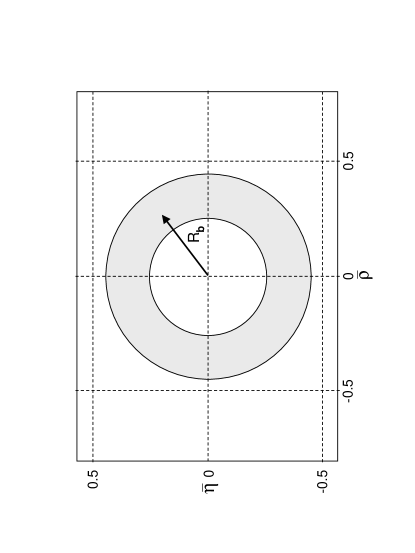
Figure 2: “Unitarity Clock”.

These two different routes for explorations of the CKM matrix and of the related unitarity triangle may answer the important question, whether the Kobayashi-Maskawa picture of CP violation is correct and more generally whether the Standard Model offers a correct description of weak decays of hadrons. Indeed, in order to answer these important questions it is essential to calculate as many branching ratios as possible, measure them experimentally and check if they all can be described by the same set of the parameters $(\lambda,A,\varrho,\eta)$. In the language of the unitarity triangle the question is whether the various curves in the $(\bar{\varrho},\bar{\eta})$ plane extracted from different decays and transitions will cross each other at a single point as shown in fig. 3 and whether the angles $(\alpha,\beta,\gamma)$ in the resulting triangle will agree with those extracted from CP-asymmetries in B decays and CP-conserving B decays. It is truely exciting that during the present decade we should be able to answer all these questions and in the case of the inconsistencies in the $(\bar{\varrho},\bar{\eta})$ plane get some hints about the physics beyond the SM. One obvious inconsistency would be the violation of the constraint (1.36).

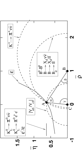
Figure 3: The ideal Unitarity Triangle.

Clearly the plot in fig. 3 is highly idealized because in order to extract such nice curves from various decays one needs perfect experiments and perfect theory. One of the goals of these lectures is to identify those decays for which at least the theory is under control. For such decays, if they can be measured with a sufficient precision, the curves in fig. 3 are not fully unrealistic. Let us then briefly discuss the theoretical framework for weak decays.

2 Theoretical Framework

2.1 OPE and Renormalization Group

The basis for any serious phenomenology of weak decays of hadrons is the Operator Product Expansion (OPE) [33, 34], which allows to write the effective weak Hamiltonian simply as follows

$${\cal H}_{eff}=\frac{G_{F}}{\sqrt{2}}\sum_{i}V^{i}_{\rm CKM}C_{i}(\mu)Q_{i}~{}.$$ (2.1)

Here $G_{F}$ is the Fermi constant and $Q_{i}$ are the relevant local operators which govern the decays in question. They are built out of quark and lepton fields. The Cabibbo-Kobayashi-Maskawa factors $V^{i}_{\rm CKM}$ [16, 17] and the Wilson coefficients $C_{i}(\mu)$ [33] describe the strength with which a given operator enters the Hamiltonian. The latter coefficients can be considered as scale dependent “couplings” related to “vertices” $Q_{i}$ and as discussed below can be calculated using perturbative methods as long as $\mu$ is not too small.

An amplitude for a decay of a given meson $M=K,B,..$ into a final state $F=\pi\nu\bar{\nu},~{}\pi\pi,~{}DK$ is then simply given by

$$A(M\to F)=\langle F|{\cal H}_{eff}|M\rangle=\frac{G_{F}}{\sqrt{2}}\sum_{i}V^{i}_{CKM}C_{i}(\mu)\langle F|Q_{i}(\mu)|M\rangle,$$ (2.2)

where $\langle F|Q_{i}(\mu)|M\rangle$ are the matrix elements of $Q_{i}$ between M and F, evaluated at the renormalization scale $\mu$.

The essential virtue of OPE is this one. It allows to separate the problem of calculating the amplitude $A(M\to F)$ into two distinct parts: the short distance (perturbative) calculation of the coefficients $C_{i}(\mu)$ and the long-distance (generally non-perturbative) calculation of the matrix elements $\langle Q_{i}(\mu)\rangle$. The scale $\mu$ separates, roughly speaking, the physics contributions into short distance contributions contained in $C_{i}(\mu)$ and the long distance contributions contained in $\langle Q_{i}(\mu)\rangle$. Thus $C_{i}$ include the top quark contributions and contributions from other heavy particles such as W-, Z-bosons and charged Higgs particles or supersymmetric particles in the supersymmetric extensions of the SM. Consequently $C_{i}(\mu)$ depend generally on $m_{t}$ and also on the masses of new particles if extensions of the SM are considered. This dependence can be found by evaluating so-called box and penguin diagrams with full W-, Z-, top- and new particles exchanges and properly including short distance QCD effects. The latter govern the $\mu$-dependence of $C_{i}(\mu)$.

The value of $\mu$ can be chosen arbitrarily but the final result must be $\mu$-independent. Therefore the $\mu$-dependence of $C_{i}(\mu)$ has to cancel the $\mu$-dependence of $\langle Q_{i}(\mu)\rangle$. In other words it is a matter of choice what exactly belongs to $C_{i}(\mu)$ and what to $\langle Q_{i}(\mu)\rangle$. This cancellation of the $\mu$-dependence involves generally several terms in the expansion in (2.2). The coefficients $C_{i}(\mu)$ depend also on the renormalization scheme. This scheme dependence must also be canceled by the one of $\langle Q_{i}(\mu)\rangle$ so that the physical amplitudes are renormalization scheme independent. Again, as in the case of the $\mu$-dependence, the cancellation of the renormalization scheme dependence involves generally several terms in the expansion (2.2).

Although $\mu$ is in principle arbitrary, it is customary to choose $\mu$ to be of the order of the mass of the decaying hadron. This is ${\cal O}(m_{\rm b})$ and ${\cal O}(m_{\rm c})$ for B decays and D decays respectively. In the case of K decays the typical choice is $\mu={\cal O}(1-2~{}\,{\rm GeV})$ instead of ${\cal O}(m_{K})$, which is much too low for any perturbative calculation of the couplings $C_{i}$. Now due to the fact that $\mu\ll M_{W,Z},~{}m_{t}$, large logarithms $\ln M_{\rm W}/\mu$ compensate in the evaluation of $C_{i}(\mu)$ the smallness of the QCD coupling constant $\alpha_{s}$ and terms $\alpha^{n}_{s}(\ln M_{\rm W}/\mu)^{n}$, $\alpha^{n}_{s}(\ln M_{\rm W}/\mu)^{n-1}$ etc. have to be resummed to all orders in $\alpha_{s}$ before a reliable result for $C_{i}$ can be obtained. This can be done very efficiently by means of the renormalization group methods. The resulting renormalization group improved perturbative expansion for $C_{i}(\mu)$ in terms of the effective coupling constant $\alpha_{s}(\mu)$ does not involve large logarithms and is more reliable. The related technical issues are discussed in detail in [1] and [3].

All this looks rather formal but in fact should be familiar. Indeed, in the simplest case of the $\beta$-decay, ${\cal H}_{eff}$ takes the familiar form

$${\cal H}^{(\beta)}_{eff}=\frac{G_{F}}{\sqrt{2}}\cos\theta_{c}[\bar{u}\gamma_{\mu}(1-\gamma_{5})d\otimes\bar{e}\gamma^{\mu}(1-\gamma_{5})\nu_{e}]~{},$$ (2.3)

where $V_{ud}$ has been expressed in terms of the Cabibbo angle. In this particular case the Wilson coefficient is equal unity and the local operator, the object between the square brackets, is given by a product of two $V-A$ currents. Equation (2.3) represents the Fermi theory for $\beta$-decays as formulated by Sudarshan and Marshak [35] and Feynman and Gell-Mann [36] more than forty years ago, except that in (2.3) the quark language has been used and following Cabibbo a small departure of $V_{ud}$ from unity has been incorporated. In this context the basic formula (2.1) can be regarded as a generalization of the Fermi Theory to include all known quarks and leptons as well as their strong and electroweak interactions as summarized by the SM.

Due to the interplay of electroweak and strong interactions the structure of the local operators is much richer than in the case of the $\beta$-decay. They can be classified with respect to the Dirac structure, colour structure and the type of quarks and leptons relevant for a given decay. Of particular interest are the operators involving quarks only. In the case of the $\Delta S=1$ transitions the relevant set of operators is given as follows:

Current–Current :

$$Q_{1}=(\bar{s}_{\alpha}u_{\beta})_{V-A}\;(\bar{u}_{\beta}d_{\alpha})_{V-A}~{}~{}~{}~{}~{}~{}Q_{2}=(\bar{s}u)_{V-A}\;(\bar{u}d)_{V-A}$$ (2.4)

QCD–Penguins :

$$Q_{3}=(\bar{s}d)_{V-A}\sum_{q=u,d,s}(\bar{q}q)_{V-A}~{}~{}~{}~{}~{}~{}Q_{4}=(\bar{s}_{\alpha}d_{\beta})_{V-A}\sum_{q=u,d,s}(\bar{q}_{\beta}q_{\alpha})_{V-A}$$ (2.5)

$$Q_{5}=(\bar{s}d)_{V-A}\sum_{q=u,d,s}(\bar{q}q)_{V+A}~{}~{}~{}~{}~{}Q_{6}=(\bar{s}_{\alpha}d_{\beta})_{V-A}\sum_{q=u,d,s}(\bar{q}_{\beta}q_{\alpha})_{V+A}$$ (2.6)

Electroweak–Penguins :

$$Q_{7}={3\over 2}\;(\bar{s}d)_{V-A}\sum_{q=u,d,s}e_{q}\;(\bar{q}q)_{V+A}~{}~{}~{}~{}~{}Q_{8}={3\over 2}\;(\bar{s}_{\alpha}d_{\beta})_{V-A}\sum_{q=u,d,s}e_{q}(\bar{q}_{\beta}q_{\alpha})_{V+A}$$ (2.7)

$$Q_{9}={3\over 2}\;(\bar{s}d)_{V-A}\sum_{q=u,d,s}e_{q}(\bar{q}q)_{V-A}~{}~{}~{}~{}~{}Q_{10}={3\over 2}\;(\bar{s}_{\alpha}d_{\beta})_{V-A}\sum_{q=u,d,s}e_{q}\;(\bar{q}_{\beta}q_{\alpha})_{V-A}\,.$$ (2.8)

Here, $\alpha,\beta$ denote colours and $e_{q}$ denotes the electric quark charges reflecting the electroweak origin of $Q_{7},\ldots,Q_{10}$. Finally, $(\bar{s}u)_{V-A}\equiv\bar{s}_{\alpha}\gamma_{\mu}(1-\gamma_{5})u_{\alpha}$.

Clearly, in order to calculate the amplitude $A(M\to F)$ the matrix elements $\langle Q_{i}(\mu)\rangle$ have to be evaluated. Since they involve long distance contributions one is forced in this case to use non-perturbative methods such as lattice calculations, the 1/N expansion (N is the number of colours), QCD sum rules, hadronic sum rules, chiral perturbation theory and so on. In the case of certain B-meson decays, the Heavy Quark Effective Theory (HQET) also turns out to be a useful tool. Needless to say, all these non-perturbative methods have some limitations. Consequently the dominant theoretical uncertainties in the decay amplitudes reside in the matrix elements $\langle Q_{i}(\mu)\rangle$.

The fact that in many cases the matrix elements $\langle Q_{i}(\mu)\rangle$ cannot be reliably calculated at present, is very unfortunate. One of the main goals of the experimental studies of weak decays is the determination of the CKM factors $V_{\rm CKM}$ and the search for the physics beyond the SM. Without a reliable estimate of $\langle Q_{i}(\mu)\rangle$ this goal cannot be achieved unless these matrix elements can be determined experimentally or removed from the final measurable quantities by taking suitable ratios and combinations of decay amplitudes or branching ratios. Flavour symmetries like $SU(2)_{\rm F}$ and $SU(3)_{\rm F}$ relating various matrix elements can be useful in this respect, provided flavour breaking effects can be reliably calculated. However, this can be achieved rarely and often one has to face directly the calculation of $\langle Q_{i}(\mu)\rangle$. We will discuss these problems later on.

One of the outstanding issues in the calculation of $\langle Q_{i}(\mu)\rangle$ is the compatibility (“matching”) of $\langle Q_{i}(\mu)\rangle$ with $C_{i}(\mu)$. $\langle Q_{i}(\mu)\rangle$ have to carry the correct $\mu$ and renormalization scheme dependence in order to ensure the $\mu$ and scheme independence of physical amplitudes. Most of the non-perturbative methods struggle still with this problem. Moreover, it has been emphasised recently in [37] that the presence of higher dimensional operators can in the case of low matching scales complicate further this issue. It appears to me that in the future lattice methods have the best chance to get the matching in question under control. On the other hand, analytic solutions would certainly be preferable.

2.2 Wilson Coefficients at NLO

In order to achieve sufficient precision for the theoretical predictions it is desirable to have accurate values of $C_{i}(\mu)$ . Indeed it has been realized at the end of the 1980’s that the leading term (LO) in the renormalization group improved perturbation theory, in which the terms $\alpha^{n}_{s}(\ln M_{\rm W}/\mu)^{n}$ are summed, is generally insufficient and the inclusion of next-to-leading corrections (NLO) corresponding to summing the terms $\alpha^{n}_{s}(\ln M_{\rm W}/\mu)^{n-1}$ is necessary. In particular, the proper matching of $C_{i}(\mu)$ and $\langle Q_{i}(\mu)\rangle$ discussed above can only be done meaningfully after NLO corrections have been taken into account. One finds then that unphysical $\mu$- and renormalization scheme dependences in the decay amplitudes and branching ratios resulting from the truncation of the perturbative series are considerably reduced by including NLO corrections. It is then instructive to discuss briefly the general formulae for $C_{i}(\mu)$ at the NLO level. Detailed exposition can be found in [3] and [1].

The general expression for $C_{i}(\mu)$ is given by:

$$\vec{C}(\mu)=\hat{U}(\mu,M_{W})\vec{C}(M_{W})$$ (2.9)

where $\vec{C}$ is a column vector built out of $C_{i}$’s. $\vec{C}(M_{W})$ are the initial conditions which depend on the short distance physics at high energy scales. In particular they depend on $m_{\rm t}$. We set the high energy scale at $M_{\rm W}$, but other choices are clearly possible. $\hat{U}(\mu,M_{W})$, the evolution matrix, is given as follows:

$$\hat{U}(\mu,M_{W})=T_{g}\exp\left[\int_{g(M_{W})}^{g(\mu)}{dg^{\prime}\frac{\hat{\gamma}^{T}(g^{\prime})}{\beta(g^{\prime})}}\right]$$ (2.10)

with $g$ denoting the QCD effective coupling constant and $T_{g}$ an ordering operation defined in [1]. $\beta(g)$ governs the evolution of $g$ and $\hat{\gamma}$ is the anomalous dimension matrix of the operators involved. The structure of this equation makes it clear that the renormalization group approach goes beyond the usual perturbation theory. Indeed $\hat{U}(\mu,M_{W})$ sums automatically large logarithms $\log M_{W}/\mu$ which appear for $\mu\ll M_{W}$. In the so-called leading logarithmic approximation (LO) terms $(g^{2}\log M_{W}/\mu)^{n}$ are summed. The next-to-leading logarithmic correction (NLO) to this result involves summation of terms $(g^{2})^{n}(\log M_{W}/\mu)^{n-1}$ and so on. This hierarchic structure gives the renormalization group improved perturbation theory.

As an example let us consider only QCD effects and the case of a single operator so that (2.9) reduces to

$$C(\mu)=U(\mu,M_{W})C(M_{W})$$ (2.11)

with $C(\mu)$ denoting the coefficient of the operator in question. Keeping the first two terms in the expansions of $\gamma(g)$ and $\beta(g)$ in powers of $g$:

$$\gamma(g)=\gamma^{(0)}\frac{\alpha_{s}}{4\pi}+\gamma^{(1)}\left(\frac{\alpha_{s}}{4\pi}\right)^{2},\quad\quad\beta(g)=-\beta_{0}\frac{g^{3}}{16\pi^{2}}-\beta_{1}\frac{g^{5}}{(16\pi^{2})^{2}}$$ (2.12)

and inserting these expansions into (2.10) gives:

$$U(\mu,M_{W})=\Biggl{[}1+{{\alpha_{s}(\mu)}\over{4\pi}}J\Biggl{]}\Biggl{[}{{\alpha_{s}(M_{W})}\over{\alpha_{s}(\mu)}}\Biggl{]}^{P}\Biggl{[}1-{{\alpha_{s}(M_{W})}\over{4\pi}}J\Biggl{]}$$ (2.13)

where

$$P={{\gamma^{(0)}}\over{2\beta_{0}}},~{}~{}~{}~{}~{}~{}~{}~{}~{}J={{P}\over{\beta_{0}}}\beta_{1}-{{\gamma^{(1)}}\over{2\beta_{0}}}.$$ (2.14)

General formulae for $\hat{U}(\mu,M_{W})$ in the case of operator mixing and valid also for electroweak effects can be found in [3]. The leading logarithmic approximation corresponds to setting $J=0$ in (2.13).

At NLO, $C(M_{\rm W})$ is given by

$$C(M_{\rm W})=C_{0}+\frac{\alpha_{s}(M_{\rm W})}{4\pi}C_{1}$$ (2.15)

where $C_{0}$ and $C_{1}$ depend generally on $m_{\rm t}$, $M_{\rm W}$ and the masses of the new particles in the extentions of the SM. It should be stressed that the renormalization scheme dependence of $C_{1}$ is canceled by the one of $J$ in the last square bracket in (2.13). The scheme dependence of J in the first square bracket in (2.13) is canceled by the scheme dependence of $\langle Q(\mu)\rangle$. The power $P$ is scheme independent. The methods for the calculation of $\hat{U}(\mu,M_{W})$ and the discussion of the cancellation of the $\mu$- and scheme dependence are presented in detail in [1].

As an example consider the case of the operator $(\bar{b}d)_{V-A}(\bar{b}d)_{V-A}$ relevant for $B^{0}_{d}-\bar{B}^{0}_{d}$ mixing. In this case using the so-called NDR renormalization scheme one has [39, 52]

$$U(m_{\rm b},M_{\rm W})=\Biggl{[}1+1.63{{\alpha_{s}(m_{\rm b})}\over{4\pi}}\Biggl{]}\Biggl{[}{{\alpha_{s}(M_{\rm W})}\over{\alpha_{s}(m_{\rm b})}}\Biggl{]}^{6/25}\Biggl{[}1-1.63{{\alpha_{s}(M_{\rm W})}\over{4\pi}}\Biggl{]}=0.86~{}.$$ (2.16)

where we have used $f=5$, $\alpha_{s}(M_{\rm Z})=0.118$ and $\alpha_{s}(m_{\rm b})=0.222$. The departure of $U(m_{\rm b},M_{\rm W})$ from unity is rather small in this example, due to the small value of the power $P$. In the case of $(V-A)\otimes(V+A)$ operators the renormalization group effects are larger.

2.3 Status of the NLO Calculations

2.3.1 General Comments

During the last decade the NLO corrections to $C_{i}(\mu)$ have been calculated within the SM for the most important and interesting decays. They will be taken into account in these lectures. In table 1 we give references to all NLO calculations within the SM done until the end of 2000. While these calculations improved considerably the precision of theoretical predictions in weak decays and can be considered as an important progress in this field, the pioneering LO calculations for current-current operators [77], penguin operators [78] and $\Delta S=2$ operators [79] should not be forgotten.

2.3.2 NNLO Calculations

In the case of the CP violating ratio $\varepsilon^{\prime}/\varepsilon$ and the rare decays $B\to X_{s}l^{+}l^{-}$ and $K_{L}\to\pi^{0}e^{+}e^{-}$, the NLO matching conditions for electroweak operators do not involve QCD corrections to box and penguin diagrams and consequently the renormalization scale dependence in the top quark mass in these processes is not negligible. In order to reduce this unphysical dependence, QCD corrections to the relevant box and penguin diagrams have to be computed. In the renormalization group improved perturbation theory these corrections are a part of next-next-to-leading (NNLO) corrections. In [80] and [81] such corrections have been computed for $\varepsilon^{\prime}/\varepsilon$ and the rare decays in question, respectively.

2.3.3 Two-Loop Anomalous Dimensions Beyond the SM

In the extentions of the SM new operators are present. The two loop anomalous dimensions for all $\Delta F=2$ four-quark dimension-six operators have been computed in [82, 83]. In [83] also the corresponding results for $\Delta F=1$ can be found. The applications of these results to $(\Delta M_{K},\varepsilon_{K})$ and $\Delta B=1$ decays in the MSSM can be found in [84] and [85], respectively.

2.3.4 Two-Loop Electroweak Corrections

In order to reduce scheme and scale dependences related to the definition of electroweak parameters like $\sin^{2}\theta_{W}$, and $\alpha_{QED}$, two-loop electroweak contributions to rare decays have to be computed. For $K^{0}_{L}\rightarrow\pi^{0}\nu\bar{\nu}$, $B\rightarrow l^{+}l^{-}$ and $B\rightarrow X_{\rm s}\nu\bar{\nu}$ they can be found in [86], for $B^{0}-\bar{B}^{0}$ mixing in [87] and for $B\rightarrow X_{s}\gamma$ in [88, 89, 90, 91].

2.3.5 NLO Calculations Beyond the SM

There exist also a number of partial or complete NLO QCD calculations within the Two-Higgs-Doublet Model and the MSSM. In the case of the Two-Higgs-Doublet Model such calculations for $B^{0}-\bar{B}^{0}$ mixing and $B\to X_{s}\gamma$ can be found in [53] and [70, 71, 92] respectively. The corresponding calculations for $B\to X_{s}\gamma$ in the MSSM can be found in [93] and [72]. The latter paper gives also the results for $B\to X_{s}{\rm gluon}$. Finally gluino-mediated NLO-QCD corrections to $B^{0}-\bar{B}^{0}$ mixing in the MSSM have been considered in [94].

Table 1: References to NLO Calculations within the SM

XXXXXXXX Decay	Reference
$\Delta F=1$ Decays
current-current operators	[38, 39]
QCD penguin operators	[40, 42, 43, 44, 45]
electroweak penguin operators	[41, 42, 43, 44]
magnetic penguin operators	[46, 47]
$Br(B)_{SL}$	[38, 48, 49]
inclusive $\Delta S=1$ decays	[50]
Particle-Antiparticle Mixing
$\eta_{1}$	[51]
$\eta_{2},~{}\eta_{B}$	[52, 53]
$\eta_{3}$	[54]
Rare $K$- and $B$-Meson Decays
$K^{0}_{L}\rightarrow\pi^{0}\nu\bar{\nu}$, $B\rightarrow l^{+}l^{-}$, $B\rightarrow X_{\rm s}\nu\bar{\nu}$	[55, 56, 57, 58]
$K^{+}\rightarrow\pi^{+}\nu\bar{\nu}$, $K_{\rm L}\rightarrow\mu^{+}\mu^{-}$	[59, 58]
$K^{+}\to\pi^{+}\mu\bar{\mu}$	[60]
$K_{\rm L}\rightarrow\pi^{0}e^{+}e^{-}$	[61]
$B\rightarrow X_{s}\mu^{+}\mu^{-}$	[62, 63]
$B\rightarrow X_{s}\gamma$	[64]-[71]
$B\rightarrow X_{s}{\rm gluon}$	[68, 72, 73]
$\Delta\Gamma_{B_{s}}$	[74]
inclusive B $\to$ Charmonium	[75]
$B\to D\pi$, $B\to\pi\pi$	[76]

2.4 QCD Factorization for Exclusive Non-Leptonic B-Meson Decays

A simple method for the evaluation of the hadronic matrix elements of four quark operators relevant for B decays is the factorization approach in which the matrix elements are expressed in terms of products of meson decay constants and formfactors [95]. In its naive formulation, this approach gives the $\mu$-independent hadronic matrix elements and consequently $\mu$-dependent decay amplitudes. Moreover final state interactions are not taken into account. Various generalizations of this method have been proposed in the literature [96] with the hope to include non-factorizable contributions and to remove the $\mu$-dependence from the decay amplitudes. Critical reviews of these attempts can be found in [97, 76]. Parallel to these efforts general parametrizations of decay amplitudes by means of flavour flow diagrams [98] and Wick contractions [99, 100] supplemented by dynamical assumptions have been proposed. These parametrizations may turn out to be useful when more data will be available.

Recently factorization for a large class of non-leptonic two-body B-meson decays has been shown by Beneke, Buchalla, Neubert and Sachrajda [76] to follow from QCD in the heavy-quark limit. The resulting factorization formula incorporates elements of the naive factorization approach but allows to compute systematically non-factorizable corrections. In this approach the $\mu$-dependence of hadronic matrix elements is under control. Moreover spectator quark effects are taken into account and final state interaction phases can be computed perturbatively. While, in my opinion, an important progress in evaluating non-leptonic amplitudes has been made in [76], the usefulness of this approach at the quantitative level has still to be demonstrated when the data improve. In particular the role of the $1/m_{b}$ corrections has to be considerably better understood. Recent lectures on this approach can be found in [101].

There is an alternative perturbative QCD approach to non-leptonic decays [102] which has been developed earlier from the QCD hard-scattering approach. Some elements of this approach are present in the QCD factorization formula of [76]. The main difference between these two approaches is the treatment of soft spectator contributions which are assumed to be negligible in the perturbative QCD approach. While the QCD factorization approach is more general and systematic, the perturbative QCD approach is an interesting possibility. Competition is always healthy and only time will show which of these two frameworks is more successful and whether they have to be replaced by still more powerful approches in the future.

Finally a new method to calculate the $B\to\pi\pi$ hadronic matrix elements from QCD light-cone sum rules has been proposed very recently by Khodjamirian [103]. This work may shed light on the importance of $1/m_{\rm b}$ and soft-gluon effects in the QCD factorization approach. Reviews of QCD light-cone sum rules can be found in [104].

2.5 Inclusive Decays

So far we have discussed only exclusive decays. It turns out that in the case of inclusive decays of heavy mesons, like B-mesons, things turn out to be easier. In an inclusive decay one sums over all or over a special class of accessible final states. A well known example is the decay $B\to X_{s}\gamma$, where $X_{s}$ includes all accessible final states with the net strange quantum number $S=1.$

At first sight things look as complicated as in the case of exclusive decays. It turns out, however, that the resulting branching ratio can be calculated in the expansion in inverse powers of $m_{\rm b}$ with the leading term described by the spectator model in which the B-meson decay is modelled by the decay of the $b$-quark:

$${\rm Br}(B\to X)={\rm Br}(b\to q)+{\cal O}(\frac{1}{m_{\rm b}^{2}})~{}.$$ (2.17)

This formula is known under the name of the Heavy Quark Expansion (HQE) [105, 106]. Since the leading term in this expansion represents the decay of the quark, it can be calculated in perturbation theory or more correctly in the renormalization group improved perturbation theory. It should be emphasized that also here the basic starting point is the effective Hamiltonian (2.1) and that the knowledge of $C_{i}(\mu)$ is essential for the evaluation of the leading term in (2.17). But there is an important difference relative to the exclusive case: the matrix elements of the operators $Q_{i}$ can be “effectively” evaluated in perturbation theory. This means, in particular, that their $\mu$ and renormalization scheme dependences can be evaluated and the cancellation of these dependences by those present in $C_{i}(\mu)$ can be explicitly investigated.

Clearly in order to complete the evaluation of $Br(B\to X)$ also the remaining terms in (2.17) have to be considered. These terms are of a non-perturbative origin, but fortunately they are suppressed by at least two powers of $m_{b}$. They have been studied by several authors in the literature [106] with the result that they affect various branching ratios by less then $10\%$ and often by only a few percent. Consequently the inclusive decays give generally more precise theoretical predictions at present than the exclusive decays. On the other hand their measurements are harder. There are of course some important theoretical issues related to the validity of HQE in (2.17) which appear in the literature under the name of quark-hadron duality. Since these matters are rather involved I will not discuss them here.

Figure 4: Typical Penguin and Box Diagrams.

2.6 Penguin–Box Expansion

The rare and CP violating decays of K and B mesons are governed by various penguin and box diagrams with internal top quark and charm quark exchanges. Some examples are shown in fig. 4. Evaluating these diagrams one finds a set of basic universal (process independent) $m_{\rm t}$-dependent functions $F_{r}(x_{t})$ [107] where $x_{t}=m_{\rm t}^{2}/M_{\rm W}^{2}$. Explicit expressions for these functions will be given below.

It is useful to express the OPE formula (2.2) directly in terms of the functions $F_{r}(x_{t})$ [108]:

$$A({M\to F})=P_{0}(M\to F)+\sum_{r}P_{r}(M\to F)\,F_{r}(x_{t}),$$ (2.18)

where the sum runs over all possible functions contributing to a given amplitude. $P_{0}$ summarizes contributions stemming from internal quarks other than the top, in particular the charm quark. In the OPE formula (2.2), the functions $F_{r}(x_{t})$ are hidden in the initial conditions for $C_{i}(\mu)$ represented by $\vec{C}(M_{\rm W})$ in (2.9).

The coefficients $P_{0}$ and $P_{r}$ are process dependent and include QCD corrections contained in the evolution matrix $\hat{U}(\mu,M_{\rm W})$. They depend also on hadronic matrix elements of local operators and the relevant CKM factors. An efficient and straightforward method for finding the coefficients $P_{r}$ is presented in [108]. I would like to call (2.18) Penguin-Box Expansion (PBE). We will encounter many examples of PBE in the course of these lectures.

Originally PBE was designed to expose the $m_{\rm t}$-dependence of FCNC processes [108]. After the top quark mass has been measured precisely this role of PBE is less important. On the other hand, PBE is very well suited for the study of the extentions of the SM in which new particles are exchanged in the loops. If there are no new local operators the mere change is to modify the functions $F_{r}(x_{t})$ which now acquire the dependence on the masses of new particles such as charged Higgs particles and supersymmetric particles. The process dependent coefficients $P_{0}$ and $P_{r}$ remain unchanged. The effects of new physics can be then transparently seen. However, if new effective operators with different Dirac and colour structures are present, new functions multiplied by new coefficients $P_{r}(M\to F)$ contribute to (2.18).

In the rest of this section we present the functions $F_{r}(x_{t})$ within the SM. To this end, let us denote by $B_{0}$, $C_{0}$ and $D_{0}$ the functions $F_{r}(x_{t})$ resulting from $\Delta F=1$ ($F$ stands for flavour) box diagram, $Z^{0}$-penguin and $\gamma$-penguin diagram respectively. These diagrams are gauge dependent and it is useful to introduce gauge independent combinations [108]

$$X_{0}=C_{0}-4B_{0},\qquad Y_{0}=C_{0}-B_{0},\qquad Z_{0}=C_{0}+\frac{1}{4}D_{0}~{}.$$ (2.19)

Then the set of gauge independent basic functions which govern the FCNC processes in the SM is given to a very good approximation as follows ($x_{i}=m^{2}_{i}/M_{\rm W}^{2}$):

$$S_{0}(x_{t})=2.46~{}\left(\frac{m_{\rm t}}{170\,{\rm GeV}}\right)^{1.52},\quad\quad S_{0}(x_{c})=x_{c},$$ (2.20)

$$S_{0}(x_{c},x_{t})=x_{c}\left[\ln\frac{x_{t}}{x_{c}}-\frac{3x_{t}}{4(1-x_{t})}-\frac{3x^{2}_{t}\ln x_{t}}{4(1-x_{t})^{2}}\right],$$ (2.21)

$$X_{0}(x_{t})=1.57~{}\left(\frac{m_{\rm t}}{170\,{\rm GeV}}\right)^{1.15},\quad\quad Y_{0}(x_{t})=1.02~{}\left(\frac{m_{\rm t}}{170\,{\rm GeV}}\right)^{1.56},$$ (2.22)

$$Z_{0}(x_{t})=0.71~{}\left(\frac{m_{\rm t}}{170\,{\rm GeV}}\right)^{1.86},\quad\quad E_{0}(x_{t})=0.26~{}\left(\frac{m_{\rm t}}{170\,{\rm GeV}}\right)^{-1.02},$$ (2.23)

$$D^{\prime}_{0}(x_{t})=0.38~{}\left(\frac{m_{\rm t}}{170\,{\rm GeV}}\right)^{0.60},\quad\quad E^{\prime}_{0}(x_{t})=0.19~{}\left(\frac{m_{\rm t}}{170\,{\rm GeV}}\right)^{0.38}.$$ (2.24)

The first three functions correspond to $\Delta F=2$ box diagrams with $(t,t)$, $(c,c)$ and $(t,c)$ exchanges. $E_{0}$ results from QCD penguin diagram with off-shell gluon, $D^{\prime}_{0}$ and $E^{\prime}_{0}$ from $\gamma$ and QCD penguins with on-shell photons and gluons respectively. The subscript “$0$” indicates that these functions do not include QCD corrections to the relevant penguin and box diagrams.

In the range $150\,{\rm GeV}\leq m_{\rm t}\leq 200\,{\rm GeV}$ these approximations reproduce the exact expressions to an accuracy better than 1%. These formulae will allow us to exhibit elegantly the $m_{\rm t}$ dependence of various branching ratios in the phenomenological sections of these lectures. Exact expressions for all functions can be found in [1].

Generally, several basic functions contribute to a given decay, although decays exist which depend only on a single function. We have the following correspondence between the most interesting FCNC processes and the basic functions:

$K^{0}-\bar{K}^{0}$-mixing		$S_{0}(x_{t})$, $S_{0}(x_{c},x_{t})$, $S_{0}(x_{c})$
$B_{d,s}^{0}-\bar{B}_{d,s}^{0}$-mixing		$S_{0}(x_{t})$
$K\to\pi\nu\bar{\nu}$, $B\to X_{d,s}\nu\bar{\nu}$		$X_{0}(x_{t})$
$K_{\rm L}\to\mu\bar{\mu}$, $B\to l\bar{l}$		$Y_{0}(x_{t})$
$K_{\rm L}\to\pi^{0}e^{+}e^{-}$		$Y_{0}(x_{t})$, $Z_{0}(x_{t})$, $E_{0}(x_{t})$
$\varepsilon^{\prime}$		$X_{0}(x_{t})$, $Y_{0}(x_{t})$, $Z_{0}(x_{t})$, $E_{0}(x_{t})$
$B\to X_{s}\gamma$		$D^{\prime}_{0}(x_{t})$, $E^{\prime}_{0}(x_{t})$
$B\to X_{s}\mu^{+}\mu^{-}$		$Y_{0}(x_{t})$, $Z_{0}(x_{t})$, $E_{0}(x_{t})$, $D^{\prime}_{0}(x_{t})$, $E^{\prime}_{0}(x_{t})$

The supersymmetric contributions to the functions $S_{0}$, $X_{0}$, $Y_{0}$, $Z_{0}$ and $E_{0}$ within the MSSM with minimal flavour violation (see Section 9) have been recently compiled in [109]. See also [110]-[113]. QCD corrections to these functions can be extracted from papers in table 1 and from the section on NLO calculations beyond the SM. In the SM it is convenient in most cases to include these corrections in the coefficients $P_{r}$. Beyond the SM it is better to retain them in $F_{r}$ as these corrections depend on the new parameters present in the extentions of the SM.

3 Particle-Antiparticle Mixing and Various Types
of CP Violation

3.1 Preliminaries

Let us next discuss the formalism of particle–antiparticle mixing and CP violation. Much more elaborate discussion can be found in two recent books [6, 7]. We will concentrate here on $K^{0}-\bar{K}^{0}$ mixing, $B_{d,s}^{0}-\bar{B}^{0}_{d,s}$ mixings and CP violation in K-meson and B-meson decays. As this section is rather long it is useful to specify our goals. These are:

• Presentation of basic concepts of particle–antiparticle mixing and CP violation.

• Introduction of the CP violating parameters $\varepsilon$ and $\varepsilon^{\prime}$ that describe the so–called indirect a direct CP violation in $K_{L}\to\pi\pi$, respectively.

• Presentation of a different and more useful classification of different types of CP violation that distinguishes between: CP violation in mixing, CP violation in decay and CP violation in the interference between mixing and decay.

• Derivation of a number of formulae that will turn out to be useful in subsequent more phenomenological sections.

It is important to emphasize at this moment that particle–antiparticle mixing and CP violation have been of fundamental importance for the construction and testing of the SM. They have also proven often to be undefeatable challenges for suggested extensions of this model. In this context the seminal papers of Glashow, Iliopoulos and Maiani [18] and of Kobayashi and Maskawa [17] should be mentioned. From the calculation of the $K_{\rm L}-K_{\rm S}$ mass difference, Gaillard and Lee [114] were able to estimate the value of the charm quark mass before charm discovery. On the other hand $B_{d}^{0}-\bar{B}_{d}^{0}$ mixing [115] gave the first indication of a large top quark mass. Next CP violation in the $K^{0}-\bar{K}^{0}$ mixing offers within the SM a plausible description of CP violation in $K_{L}\to\pi\pi$ discovered in 1964 [32]. Finally the very small values of the measured $K_{\rm L}-K_{\rm S}$ mass difference and of the CP violating parameter $\varepsilon$ put severe restrictions on the flavour structure and the pattern of complex phases in the extentions of the SM. This is in particular the case of general supersymmetric extentions of the SM, in which the mismatch in the alignment of the quark mass matrices and the squark mass matrices is very restricted by the $K_{\rm L}-K_{\rm S}$ mass difference and $\varepsilon$.

It is important to stress that in the SM the phenomena discussed in this section appear first at the one–loop level and as such they are sensitive measures of the top quark couplings $V_{ti}(i=d,s,b)$ and in particular of the phase $\delta=\gamma$. They allow then to construct the unitarity triangle as explicitly demonstrated in Section 4.

Let us next enter some details. The following subsection borrows a lot from [116, 117]. The discussion of different types of CP violation benefited from several very nice lectures by Nir [118], although the presentation of this topic below differs occassionally from his.

Figure 5: Box diagrams contributing to $K^{0}-\bar{K}^{0}$ mixing in the SM.

3.2 Express Review of $K^{0}-\bar{K}^{0}$ Mixing

$K^{0}=(\bar{s}d)$ and $\bar{K}^{0}=(s\bar{d})$ are flavour eigenstates which in the SM may mix via weak interactions through the box diagrams in fig. 5. We will choose the phase conventions so that

$$CP|K^{0}\rangle=-|\bar{K}^{0}\rangle,\qquad CP|\bar{K}^{0}\rangle=-|K^{0}\rangle.$$ (3.1)

In the absence of mixing the time evolution of $|K^{0}(t)\rangle$ is given by

$$|K^{0}(t)\rangle=|K^{0}(0)\rangle\exp(-iHt)~{},\qquad H=M-i\frac{\Gamma}{2}~{},$$ (3.2)

where $M$ is the mass and $\Gamma$ the width of $K^{0}$. Similar formula exists for $\bar{K}^{0}$.

On the other hand, in the presence of flavour mixing the time evolution of the $K^{0}-\bar{K}^{0}$ system is described by

$$i\frac{d\psi(t)}{dt}=\hat{H}\psi(t)\qquad\psi(t)=\left(\begin{array}[]{c}|K^{0}(t)\rangle\\ |\bar{K}^{0}(t)\rangle\end{array}\right)$$ (3.3)

where

$$\hat{H}=\hat{M}-i\frac{\hat{\Gamma}}{2}=\left(\begin{array}[]{cc}M_{11}-i\frac{\Gamma_{11}}{2}&M_{12}-i\frac{\Gamma_{12}}{2}\\ M_{21}-i\frac{\Gamma_{21}}{2}&M_{22}-i\frac{\Gamma_{22}}{2}\end{array}\right)$$ (3.4)

with $\hat{M}$ and $\hat{\Gamma}$ being hermitian matrices having positive (real) eigenvalues in analogy with $M$ and $\Gamma$. $M_{ij}$ and $\Gamma_{ij}$ are the transition matrix elements from virtual and physical intermediate states respectively. Using

$$M_{21}=M^{*}_{12}~{},\qquad\Gamma_{21}=\Gamma_{12}^{*}~{},\quad\quad{\rm(hermiticity)}$$ (3.5)

$$M_{11}=M_{22}\equiv M~{},\qquad\Gamma_{11}=\Gamma_{22}\equiv\Gamma~{},\quad{\rm(CPT)}$$ (3.6)

we have

$$\hat{H}=\left(\begin{array}[]{cc}M-i\frac{\Gamma}{2}&M_{12}-i\frac{\Gamma_{12}}{2}\\ M^{*}_{12}-i\frac{\Gamma^{*}_{12}}{2}&M-i\frac{\Gamma}{2}\end{array}\right)~{}.$$ (3.7)

Diagonalizing (3.3) we find:

Eigenstates:

$$K_{L,S}=\frac{(1+\bar{\varepsilon})K^{0}\pm(1-\bar{\varepsilon})\bar{K}^{0}}{\sqrt{2(1+\mid\bar{\varepsilon}\mid^{2})}}$$ (3.8)

where $\bar{\varepsilon}$ is a small complex parameter given by

$$\frac{1-\bar{\varepsilon}}{1+\bar{\varepsilon}}=\sqrt{\frac{M^{*}_{12}-i\frac{1}{2}\Gamma^{*}_{12}}{M_{12}-i\frac{1}{2}\Gamma_{12}}}=\frac{\Delta M-i\frac{1}{2}\Delta\Gamma}{2M_{12}-i\Gamma_{12}}=\frac{2M^{*}_{12}-i\Gamma^{*}_{12}}{\Delta M-i\frac{1}{2}\Delta\Gamma}\equiv r\exp(i\kappa)~{}.$$ (3.9)

with $\Delta\Gamma$ and $\Delta M$ given below.

Eigenvalues:

$$M_{L,S}=M\pm{\rm Re}Q\qquad\Gamma_{L,S}=\Gamma\mp 2{\rm Im}Q$$ (3.10)

where

$$Q=\sqrt{(M_{12}-i\frac{1}{2}\Gamma_{12})(M^{*}_{12}-i\frac{1}{2}\Gamma^{*}_{12})}.$$ (3.11)

Consequently we have

$$\Delta M=M_{L}-M_{S}=2{\rm Re}Q~{},\quad\quad\Delta\Gamma=\Gamma_{L}-\Gamma_{S}=-4{\rm Im}Q.$$ (3.12)

It should be noted that the mass eigenstates $K_{S}$ and $K_{L}$ differ from CP eigenstates

$$K_{1}={1\over{\sqrt{2}}}(K^{0}-\bar{K}^{0}),\qquad\qquad CP|K_{1}\rangle=|K_{1}\rangle~{},$$ (3.13)

$$K_{2}={1\over{\sqrt{2}}}(K^{0}+\bar{K}^{0}),\qquad\qquad CP|K_{2}\rangle=-|K_{2}\rangle~{},$$ (3.14)

by a small admixture of the other CP eigenstate:

$$K_{\rm S}={{K_{1}+\bar{\varepsilon}K_{2}}\over{\sqrt{1+\mid\bar{\varepsilon}\mid^{2}}}},\qquad K_{\rm L}={{K_{2}+\bar{\varepsilon}K_{1}}\over{\sqrt{1+\mid\bar{\varepsilon}\mid^{2}}}}\,.$$ (3.15)

Since $\bar{\varepsilon}$ is ${\cal O}(10^{-3})$, one has to a very good approximation:

$$\Delta M_{K}=2{\rm Re}M_{12},\qquad\Delta\Gamma_{K}=2{\rm Re}\Gamma_{12}~{},$$ (3.16)

where we have introduced the subscript K to stress that these formulae apply only to the $K^{0}-\bar{K}^{0}$ system.

The $K_{\rm L}-K_{\rm S}$ mass difference is experimentally measured to be [24]

$$\Delta M_{K}=M(K_{\rm L})-M(K_{\rm S})=(3.489\pm 0.008)\cdot 10^{-15}\,{\rm GeV}\,.$$ (3.17)

In the SM roughly $70\%$ of the measured $\Delta M_{K}$ is described by the real parts of the box diagrams with charm quark and top quark exchanges, whereby the contribution of the charm exchanges is by far dominant. This is related to the smallness of the real parts of the CKM top quark couplings compared with the corresponding charm quark couplings. Some non-negligible contribution comes from the box diagrams with simultaneous charm and top exchanges. The remaining $20\%$ of the measured $\Delta M_{K}$ is attributed to long distance contributions which are difficult to estimate [119]. Further information with the relevant references can be found in [51].

The situation with $\Delta\Gamma_{K}$ is rather different. It is fully dominated by long distance effects. Experimentally one has $\Delta\Gamma_{K}\approx-2\Delta M_{K}$. We will use this relation in what follows.

Generally to observe CP violation one needs an interference between various amplitudes that carry complex phases. As these phases are obviously convention dependent, the CP-violating effects depend only on the differences of these phases. In this context it should be stressed that the small parameter $\bar{\varepsilon}$ depends on the phase convention chosen for $K^{0}$ and $\bar{K}^{0}$. Therefore it may not be taken as a physical measure of CP violation. On the other hand ${\rm Re}~{}\bar{\varepsilon}$ and $r$, defined in (3.9) are independent of phase conventions. In particular the departure of $r$ from 1 measures CP violation in the $K^{0}-\bar{K}^{0}$ mixing:

$$r=1+\frac{2|\Gamma_{12}|^{2}}{4|M_{12}|^{2}+|\Gamma_{12}|^{2}}{\rm Im}\left(\frac{M_{12}}{\Gamma_{12}}\right)\approx 1+{\rm Im}\left(\frac{M_{12}}{\Gamma_{12}}\right)~{}.$$ (3.18)

This type of CP violation can be best isolated in semi-leptonic decays of the $K_{L}$ meson. The non-vanishing asymmetry

$$a_{\rm SL}(K_{L})=\frac{\Gamma(K_{L}\to\pi^{-}e^{+}\nu_{e})-\Gamma(K_{L}\to\pi^{+}e^{-}\bar{\nu}_{e})}{\Gamma(K_{L}\to\pi^{-}e^{+}\nu_{e})+\Gamma(K_{L}\to\pi^{+}e^{-}\bar{\nu}_{e})}=\left({\rm Im}\frac{\Gamma_{12}}{M_{12}}\right)_{K}$$ (3.19)

signals this type of CP violation. Equivalently

$$a_{SL}(\rm K_{L})=\frac{1-r^{2}}{1+r^{2}}=2{\rm Re}\bar{\varepsilon}$$ (3.20)

Note that $a_{SL}(\rm K_{L})$ is determined purely by the quantities related to $K^{0}-\bar{K}^{0}$ mixing. Specifically, it measures the difference between the phases of $\Gamma_{12}$ and $M_{12}$.

That a non–vanishing $a_{\rm SL}(K_{L})$ is indeed a signal of CP violation can also be understood in the following manner. $K_{L}$, that should be a CP eigenstate $K_{2}$ in the case of CP conservation, decays into CP conjugate final states with different rates. As ${\rm Re}\bar{\varepsilon}>0$, $K_{L}$ prefers slightly to decay into $\pi^{-}e^{+}\nu_{e}$ than $\pi^{+}e^{-}\bar{\nu}_{e}$. This would not be possible in a CP-conserving world.

3.3 The First Look at $\varepsilon$ and $\varepsilon^{\prime}$

Since a two pion final state is CP even while a three pion final state is CP odd, $K_{\rm S}$ and $K_{\rm L}$ preferably decay to $2\pi$ and $3\pi$, respectively via the following CP-conserving decay modes [120]:

$$K_{\rm L}\to 3\pi{\rm~{}~{}(via~{}K_{2}),}\qquad K_{\rm S}\to 2\pi{\rm~{}~{}(via~{}K_{1}).}$$ (3.21)

This difference is responsible for the large disparity in their life-times. A factor of 579. However, $K_{\rm L}$ and $K_{\rm S}$ are not CP eigenstates and may decay with small branching fractions as follows:

$$K_{\rm L}\to 2\pi{\rm~{}~{}(via~{}K_{1}),}\qquad K_{\rm S}\to 3\pi{\rm~{}~{}(via~{}K_{2}).}$$ (3.22)

This violation of CP is called indirect as it proceeds not via explicit breaking of the CP symmetry in the decay itself but via the admixture of the CP state with opposite CP parity to the dominant one. The measure for this indirect CP violation is defined as (I=isospin)

$$\varepsilon={{A(K_{\rm L}\rightarrow(\pi\pi)_{I=0}})\over{A(K_{\rm S}\rightarrow(\pi\pi)_{I=0})}}.$$ (3.23)

Following the derivation in [116] one finds

$$\varepsilon=\bar{\varepsilon}+i\xi=\frac{\exp(i\pi/4)}{\sqrt{2}\Delta M_{K}}\,\left({\rm Im}M_{12}+2\xi{\rm Re}M_{12}\right),\quad\quad\xi=\frac{{\rm Im}A_{0}}{{\rm Re}A_{0}}.$$ (3.24)

The phase convention dependence of the term involving $\xi$ cancells the convention dependence of $\bar{\varepsilon}$ so that $\varepsilon$ is free from this dependence. The isospin amplitude $A_{0}$ is defined below.

The important point in the definition (3.23) is that only the transition to $(\pi\pi)_{I=0}$ enters. The transition to $(\pi\pi)_{I=2}$ is absent. This allows to remove a certain type of CP violation that originates in decays only. Yet as $\varepsilon\not=\bar{\varepsilon}$ and only ${\rm Re}\varepsilon={\rm Re}\bar{\varepsilon}$, it is clear that $\varepsilon$ includes a type of CP violation represented by ${\rm Im}\varepsilon$ which is absent in the semileptonic asymmetry (3.19). We will identify this type of CP violation in Section 3.7, where a more systematic classification of different types of CP violation will be given.

Figure 6: Indirect versus direct CP violation in $K_{L}\to\pi\pi$.

While indirect CP violation reflects the fact that the mass eigenstates are not CP eigenstates, so-called direct CP violation is realized via a direct transition of a CP odd to a CP even state or vice versa (see fig. 6). A measure of such a direct CP violation in $K_{L}\to\pi\pi$ is characterized by a complex parameter $\varepsilon^{\prime}$ defined as

$$\varepsilon^{\prime}=\frac{1}{\sqrt{2}}\left(\frac{A_{2,L}}{A_{0,S}}-\frac{A_{2,S}}{A_{0,S}}\frac{A_{0,L}}{A_{0,S}}\right)$$ (3.25)

where short hand notation $A_{I,L}\equiv A(K_{L}\to(\pi\pi)_{I})$ and $A_{I,S}\equiv A(K_{S}\to(\pi\pi)_{I})$ has been used.

This time the transitions to $(\pi\pi)_{I=0}$ and $(\pi\pi)_{I=2}$ are included which allows to study CP violation in the decay itself. We will discuss this issue in general terms in Section 3.7. For the time being it is useful to cast (3.25) into a more transparent formula

$$\varepsilon^{\prime}=\frac{1}{\sqrt{2}}{\rm Im}\left(\frac{A_{2}}{A_{0}}\right)\exp(i\Phi_{\varepsilon^{\prime}}),\qquad\Phi_{\varepsilon^{\prime}}=\frac{\pi}{2}+\delta_{2}-\delta_{0},$$ (3.26)

where the isospin amplitudes $A_{I}$ in $K\to\pi\pi$ decays are introduced through

$$A(K^{+}\rightarrow\pi^{+}\pi^{0})=\sqrt{3\over 2}A_{2}e^{i\delta_{2}}~{},$$ (3.27)

$$A(K^{0}\rightarrow\pi^{+}\pi^{-})=\sqrt{2\over 3}A_{0}e^{i\delta_{0}}+\sqrt{1\over 3}A_{2}e^{i\delta_{2}}~{},$$ (3.28)

$$A(K^{0}\rightarrow\pi^{0}\pi^{0})=\sqrt{2\over 3}A_{0}e^{i\delta_{0}}-2\sqrt{1\over 3}A_{2}e^{i\delta_{2}}\,.$$ (3.29)

Here the subscript $I=0,2$ denotes states with isospin $0,2$ equivalent to $\Delta I=1/2$ and $\Delta I=3/2$ transitions, respectively, and $\delta_{0,2}$ are the corresponding strong phases. The weak CKM phases are contained in $A_{0}$ and $A_{2}$. The isospin amplitudes $A_{I}$ are complex quantities which depend on phase conventions. On the other hand, $\varepsilon^{\prime}$ measures the difference between the phases of $A_{2}$ and $A_{0}$ and is a physical quantity. The strong phases $\delta_{0,2}$ can be extracted from $\pi\pi$ scattering. Then $\Phi_{\varepsilon^{\prime}}\approx\pi/4$.

Experimentally $\varepsilon$ and $\varepsilon^{\prime}$ can be found by measuring the ratios

$$\eta_{00}={{A(K_{\rm L}\to\pi^{0}\pi^{0})}\over{A(K_{\rm S}\to\pi^{0}\pi^{0})}},\qquad\eta_{+-}={{A(K_{\rm L}\to\pi^{+}\pi^{-})}\over{A(K_{\rm S}\to\pi^{+}\pi^{-})}}.$$ (3.30)

Indeed, assuming $\varepsilon$ and $\varepsilon^{\prime}$ to be small numbers one finds

$$\eta_{00}=\varepsilon-{{2\varepsilon^{\prime}}\over{1-\sqrt{2}\omega}},~{}~{}~{}~{}\eta_{+-}=\varepsilon+{{\varepsilon^{\prime}}\over{1+\omega/\sqrt{2}}}$$ (3.31)

where $\omega={\rm Re}A_{2}/{\rm Re}A_{0}=0.045$.

In the absence of direct CP violation $\eta_{00}=\eta_{+-}$. The ratio ${\varepsilon^{\prime}}/{\varepsilon}$ can then be measured through

$${\rm Re}(\varepsilon^{\prime}/\varepsilon)=\frac{1}{6(1+\omega/\sqrt{2})}\left(1-\left|{{\eta_{00}}\over{\eta_{+-}}}\right|^{2}\right)~{}.$$ (3.32)

To my knowledge [121] the experimental groups in giving their results for ${\rm Re}(\varepsilon^{\prime}/\varepsilon)$ omitt the term $\omega/\sqrt{2}$ in (3.32). Yet in order to be consistent with the definitions (3.23) and (3.25) used by theorists this term should be kept. Consequently the existing experimental results for ${\rm Re}(\varepsilon^{\prime}/\varepsilon)$ quoted below should be rescaled down by $3.2\%$. Clearly at present this rescaling is academic as the experimental error in ${\rm Re}(\varepsilon^{\prime}/\varepsilon)$ is roughly $\pm 20\%$ and the theoretical one at least $\pm 50\%$. We will therefore omitt this rescaling in what follows.

3.4 Basic Formula for $\varepsilon$

With all this information at hand let us derive a formula for $\varepsilon$ which can be efficiently used in pheneomenological applications. The off-diagonal element $M_{12}$ in the neutral $K$-meson mass matrix representing $K^{0}$-$\bar{K}^{0}$ mixing is given by

$$2m_{K}M^{*}_{12}=\langle\bar{K}^{0}|{\cal H}_{\rm eff}(\Delta S=2)|K^{0}\rangle\,,$$ (3.33)

where ${\cal H}_{\rm eff}(\Delta S=2)$ is the effective Hamiltonian for the $\Delta S=2$ transitions. That $M^{*}_{12}$ and not $M_{12}$ stands on the l.h.s of this formula, is evident from (3.7). The factor $2m_{K}$ reflects our normalization of external states.

To lowest order in electroweak interactions $\Delta S=2$ transitions are induced through the box diagrams of fig. 5. Including leading and next-to-leading QCD corrections in the renormalization group improved perturbation theory one has for $\mu<\mu_{c}={\cal O}(m_{c})$

$${\cal H}^{\Delta S=2}_{\rm eff} = \frac{G^{2}_{\rm F}}{16\pi^{2}}M^{2}_{W}\left[\lambda^{2}_{c}\eta_{1}S_{0}(x_{c})+\lambda^{2}_{t}\eta_{2}S_{0}(x_{t})+2\lambda_{c}\lambda_{t}\eta_{3}S_{0}(x_{c},x_{t})\right]\times$$ (3.34)

$$\times\left[\alpha_{s}^{(3)}(\mu)\right]^{-2/9}\left[1+\frac{\alpha_{s}^{(3)}(\mu)}{4\pi}J_{3}\right]Q(\Delta S=2)+h.c.$$

where $\lambda_{i}=V_{is}^{*}V_{id}$, $\alpha_{s}^{(3)}$ is the strong coupling constant in an effective three flavour theory and $J_{3}=1.895$ in the NDR scheme [52]. In (3.34), the relevant operator

$$Q(\Delta S=2)=(\bar{s}d)_{V-A}(\bar{s}d)_{V-A},$$ (3.35)

is multiplied by the corresponding Wilson coefficient function. This function is decomposed into a charm-, a top- and a mixed charm-top contribution. The functions $S_{0}$ are given in (2.20) and (2.21).

Short-distance QCD effects are described through the correction factors $\eta_{1}$, $\eta_{2}$, $\eta_{3}$ and the explicitly $\alpha_{s}$-dependent terms in (3.34). The NLO values of $\eta_{i}$ are given as follows [51, 52, 54]:

$$\eta_{1}=1.38\pm 0.20,\qquad\eta_{2}=0.57\pm 0.01,\qquad\eta_{3}=0.47\pm 0.04~{}.$$ (3.36)

The quoted errors reflect the remaining theoretical uncertainties due to leftover $\mu$-dependences at ${\cal O}(\alpha_{s}^{2})$ and $\Lambda_{\overline{MS}}$, the scale in the QCD running coupling.

Defining the renormalization group invariant parameter $\hat{B}_{K}$ by

$$\hat{B}_{K}=B_{K}(\mu)\left[\alpha_{s}^{(3)}(\mu)\right]^{-2/9}\,\left[1+\frac{\alpha_{s}^{(3)}(\mu)}{4\pi}J_{3}\right]~{},$$ (3.37)

$$\langle\bar{K}^{0}|(\bar{s}d)_{V-A}(\bar{s}d)_{V-A}|K^{0}\rangle\equiv\frac{8}{3}B_{K}(\mu)F_{K}^{2}m_{K}^{2}$$ (3.38)

and using (3.34) one finds

$$M_{12}=\frac{G_{\rm F}^{2}}{12\pi^{2}}F_{K}^{2}\hat{B}_{K}m_{K}M_{\rm W}^{2}\left[{\lambda_{c}^{*}}^{2}\eta_{1}S_{0}(x_{c})+{\lambda_{t}^{*}}^{2}\eta_{2}S_{0}(x_{t})+2{\lambda_{c}^{*}}{\lambda_{t}^{*}}\eta_{3}S_{0}(x_{c},x_{t})\right],$$ (3.39)

where $F_{K}=160~{}\,{\rm MeV}$ is the $K$-meson decay constant and $m_{K}$ the $K$-meson mass. It should be mentioned that in the normalization of external states in which the factor $2m_{K}$ in (3.33) is absent, the r.h.s of (3.38) is divided by $2m_{K}$ so that (3.39) remains unchanged.

To proceed further we neglect the last term in (3.24) as it constitutes at most a 2 % correction to $\varepsilon$. This is justified in view of other uncertainties, in particular those connected with $\hat{B}_{K}$. Inserting (3.39) into (3.24) we find

$$\varepsilon=C_{\varepsilon}\hat{B}_{K}{\rm Im}\lambda_{t}\left\{{\rm Re}\lambda_{c}\left[\eta_{1}S_{0}(x_{c})-\eta_{3}S_{0}(x_{c},x_{t})\right]-{\rm Re}\lambda_{t}\eta_{2}S_{0}(x_{t})\right\}\exp(i\pi/4)\,,$$ (3.40)

where we have used the unitarity relation ${\rm Im}\lambda_{c}^{*}={\rm Im}\lambda_{t}$ and have neglected ${\rm Re}\lambda_{t}/{\rm Re}\lambda_{c}={\cal O}(\lambda^{4})$ in evaluating ${\rm Im}(\lambda_{c}^{*}\lambda_{t}^{*})$. The numerical constant $C_{\varepsilon}$ is given by

$$C_{\varepsilon}=\frac{G_{\rm F}^{2}F_{K}^{2}m_{K}M_{\rm W}^{2}}{6\sqrt{2}\pi^{2}\Delta M_{K}}=3.837\cdot 10^{4}\,.$$ (3.41)

To this end we have used the experimental value of $\Delta M_{K}$ in (3.17) and $M_{\rm W}=80.4~{}\,{\rm GeV}$.

Using the standard parametrization of (1.5) to evaluate ${\rm Im}\lambda_{i}$ and ${\rm Re}\lambda_{i}$, setting the values for $s_{12}$, $s_{13}$, $s_{23}$ and $m_{\rm t}$ in accordance with experiment and taking a value for $\hat{B}_{K}$ (see below), one can determine the phase $\delta$ by comparing (3.40) with the experimental value for $\varepsilon$

$$\varepsilon_{exp}=(2.280\pm 0.013)\cdot 10^{-3}\;\exp{i\Phi_{\varepsilon}},\qquad\Phi_{\varepsilon}={\pi\over 4}.$$ (3.42)

Once $\delta$ has been determined in this manner one can find the apex $(\bar{\varrho},\bar{\eta})$ of the unitarity triangle in fig. 1 by using

$$\varrho=\frac{s_{13}}{s_{12}s_{23}}\cos\delta,\qquad\eta=\frac{s_{13}}{s_{12}s_{23}}\sin\delta$$ (3.43)

and

$$\bar{\varrho}=\varrho(1-\frac{\lambda^{2}}{2}),\qquad\bar{\eta}=\eta(1-\frac{\lambda^{2}}{2}).$$ (3.44)

For a given set ($s_{12}$, $s_{13}$, $s_{23}$, $m_{\rm t}$, $\hat{B}_{K}$) there are two solutions for $\delta$ and consequently two solutions for $(\bar{\varrho},\bar{\eta})$. This will be evident from the analysis of the unitarity triangle discussed in detail below.

Finally we have to say a few words about the non-perturbative parameter $\hat{B}_{K}$, the main uncertainty in this analysis. References to older estimates can be found in [2]. In our numerical analysis presented below we will use

$$\hat{B}_{K}=0.85\pm 0.15\,$$ (3.45)

which is very close to most recent lattice estimates, reviewed recently in [122, 123], slightly higher that the large-N estimates [124, 125, 126] and somewhat lower than chiral quark model estimates [127].

Recently an interesting large-N calculation of $\hat{B}_{K}$ in the chiral limit and including next-to-leading 1/N corrections has been performed by Peris and de Rafael [128]. The nice feature of this calculation is the explicit cancellation of the $\mu$-dependence and the renormalization scheme dependence between the Wilson coefficient and the matrix element of the operator $Q(\Delta S=2)$. The resulting $\hat{B}_{K}=0.41\pm 0.09$ is by a factor of two lower than the value in (3.45) and the lattice results. However, before a meaningful comparision with the lattice values can be made, higher order corrections in the chiral expansion have to be added to the result in [128].

3.5 Express Review of $B_{d,s}^{0}$-$\bar{B}_{d,s}^{0}$ Mixing

The flavour eigenstates in this case are

$$B^{0}_{d}=(\bar{b}d),\qquad\bar{B}^{0}_{d}=(b\bar{d}),\qquad B^{0}_{s}=(\bar{b}s),\qquad\bar{B}^{0}_{s}=(b\bar{s})~{}.$$ (3.46)

They mix via the box diagrams in fig. 5 with $s$ replaced by $b$ in the case of $B_{d}^{0}$-$\bar{B}_{d}^{0}$ mixing. In the case $B_{s}^{0}$-$\bar{B}_{s}^{0}$ mixing also $d$ has to be replaced by $s$.

Dropping the subscripts $(d,s)$ for a moment, it is customary to denote the mass eigenstates by

$$B_{H}=pB^{0}+q\bar{B}^{0},\qquad B_{L}=pB^{0}-q\bar{B}^{0}$$ (3.47)

where

$$p=\frac{1+\bar{\varepsilon}_{B}}{\sqrt{2(1+|\bar{\varepsilon}_{B}|^{2})}},\qquad q=\frac{1-\bar{\varepsilon}_{B}}{\sqrt{2(1+|\bar{\varepsilon}_{B}|^{2})}},$$ (3.48)

with $\bar{\varepsilon}_{B}$ corresponding to $\bar{\varepsilon}$ in the $K^{0}-\bar{K}^{0}$ system. Here “H” and “L” denote Heavy and Light respectively. As in the $B^{0}-\bar{B}^{0}$ system one has $\Delta\Gamma\ll\Delta M$, it is more suitable to distinguish the mass eigenstates by their masses than the corresponding life-times.

The strength of the $B^{0}_{d,s}-\bar{B}^{0}_{d,s}$ mixings is described by the mass differences

$$\Delta M_{d,s}=M_{H}^{d,s}-M_{L}^{d,s}~{}.$$ (3.49)

In contrast to $\Delta M_{K}$ , in this case the long distance contributions are estimated to be very small and $\Delta M_{d,s}$ is very well approximated by the relevant box diagrams. Moreover, due $m_{u,c}\ll m_{t}$ only the top sector can contribute significantly to $B_{d,s}^{0}-\bar{B}_{d,s}^{0}$ mixings. The charm sector and the mixed top-charm contributions are entirely negligible.

$\Delta M_{d,s}$ can be expressed in terms of the off-diagonal element in the neutral B-meson mass matrix by using the formulae developed previously for the K-meson system. One finds

$$\Delta M_{q}=2|M_{12}^{(q)}|,\qquad q=d,s.$$ (3.50)

This formula differs from $\Delta M_{K}=2{\rm Re}M_{12}$ because in the B-system $\Gamma_{12}\ll M_{12}$.

We also have

$$\Delta\Gamma=\Gamma(B_{H})-\Gamma(B_{L})=2\frac{{\rm Re}(M_{12}\Gamma_{12}^{*})}{|M_{12}|}$$ (3.51)

and

$$\frac{q}{p}==\frac{2M^{*}_{12}-i\Gamma^{*}_{12}}{\Delta M-i\frac{1}{2}\Delta\Gamma}=\frac{M_{12}^{*}}{|M_{12}|}\left[1-\frac{1}{2}{\rm Im}\left(\frac{\Gamma_{12}}{M_{12}}\right)\right]$$ (3.52)

where higher order terms in the small quantity $\Gamma_{12}/M_{12}$ have been neglected.

The smallness of ${\rm Im}(\Gamma_{12}/M_{12})<{\cal O}(10^{-3})$ has two important consequences:

• The semileptonic asymmetry $a_{\rm SL}(B)$ discussed a few pages below is even smaller than $a_{\rm SL}(K_{L})$. Typically ${\cal O}(10^{-4})$. These are bad news.

• The ratio $q/p$ is a pure phase to an excellent approximation. These are very good news as we will see below.

Inspecting the relevant box diagrams we find

$$(M_{12}^{*})_{d}\propto(V_{td}V_{tb}^{*})^{2}~{},\qquad(M_{12}^{*})_{s}\propto(V_{ts}V_{tb}^{*})^{2}~{}.$$ (3.53)

Now, from Section 1 we know that

$$V_{td}=|V_{td}|e^{-i\beta},\qquad V_{ts}=-|V_{ts}|e^{-i\beta_{s}}$$ (3.54)

with $\beta_{s}={\cal O}(10^{-2})$. Consequently to an excellent approximation

$$\left(\frac{q}{p}\right)_{d,s}=e^{i2\phi_{M}^{d,s}},\qquad\phi^{d}_{M}=-\beta,\qquad\phi^{s}_{M}=-\beta_{s},$$ (3.55)

with $\phi_{M}^{d,s}$ given entirely by the weak phases in the CKM matrix.

3.6 Basic Formulae for $\Delta M_{d,s}$

Let us next find $\Delta M_{d,s}$. The off-diagonal term $M_{12}$ in the neutral $B$-meson mass matrix is given by a formula analogous to (3.33)

$$2m_{B_{q}}|M_{12}^{(q)}|=|\langle\bar{B}^{0}_{q}|{\cal H}_{\rm eff}(\Delta B=2)|B^{0}_{q}\rangle|,$$ (3.56)

where in the case of $B_{d}^{0}-\bar{B}_{d}^{0}$ mixing

$${\cal H}^{\Delta B=2}_{\rm eff} = \frac{G^{2}_{\rm F}}{16\pi^{2}}M^{2}_{W}\left(V^{\ast}_{tb}V_{td}\right)^{2}\eta_{B}S_{0}(x_{t})\times$$ (3.57)

$$\times\left[\alpha^{(5)}_{s}(\mu_{b})\right]^{-6/23}\left[1+\frac{\alpha^{(5)}_{s}(\mu_{b})}{4\pi}J_{5}\right]Q(\Delta B=2)+h.c.$$

Here $\mu_{b}={\cal O}(m_{b})$, $J_{5}=1.627$,

$$Q(\Delta B=2)=(\bar{b}d)_{V-A}(\bar{b}d)_{V-A}$$ (3.58)

and [52, 53]

$$\eta_{B}=0.55\pm 0.01.$$ (3.59)

In the case of $B_{s}^{0}-\bar{B}_{s}^{0}$ mixing one should simply replace $d\to s$ in (3.57) and (3.58) with all other quantities and numerical values unchanged.

Defining the renormalization group invariant parameters $\hat{B}_{q}$ in analogy to (3.37) and (3.38) one finds using (3.57)

$$\Delta M_{q}=\frac{G_{\rm F}^{2}}{6\pi^{2}}\eta_{B}m_{B_{q}}(\hat{B}_{B_{q}}F_{B_{q}}^{2})M_{\rm W}^{2}S_{0}(x_{t})|V_{tq}|^{2},$$ (3.60)

where $F_{B_{q}}$ is the $B_{q}$-meson decay constant. This implies two useful formulae

$$\Delta M_{d}=0.50/{\rm ps}\cdot\left[\frac{\sqrt{\hat{B}_{B_{d}}}F_{B_{d}}}{200\,{\rm MeV}}\right]^{2}\left[\frac{\overline{m}_{\rm t}(m_{\rm t})}{170\,{\rm GeV}}\right]^{1.52}\left[\frac{|V_{td}|}{8.8\cdot 10^{-3}}\right]^{2}\left[\frac{\eta_{B}}{0.55}\right]$$ (3.61)

and

$$\Delta M_{s}=15.1/{\rm ps}\cdot\left[\frac{\sqrt{\hat{B}_{B_{s}}}F_{B_{s}}}{240\,{\rm MeV}}\right]^{2}\left[\frac{\overline{m}_{\rm t}(m_{\rm t})}{170\,{\rm GeV}}\right]^{1.52}\left[\frac{|V_{ts}|}{0.040}\right]^{2}\left[\frac{\eta_{B}}{0.55}\right]\,.$$ (3.62)

There is a vast literature on the calculations of $F_{B_{d,s}}$ and $\hat{B}_{d,s}$. The most recent lattice results are summarized in [129, 123]. They are compatible with the results obtained with the help of QCD sum rules [130]. Guided by [129, 123] we will use in our numerical analysis the value for $F_{B_{d}}\sqrt{\hat{B}_{B_{d}}}$ given in table 2. The experimental situation on $\Delta M_{d,s}$ is also given there.

3.7 Classification of CP Violation

3.7.1 Preliminaries

We have mentioned in Section 2 that due to the presence of hadronic matrix elements, various decay amplitudes contain large theoretical uncertainties. It is of interest to investigate which measurements of CP-violating effects do not suffer from hadronic uncertainties. To this end it is useful to make a classification of CP-violating effects that is more transparent than the division into the indirect and direct CP violation considered so far. To my knowledge this classification has been developed first for B decays but it can also be useful for K decays. A nice detailed presentation can be found in [131].

Generally complex phases may enter particle–antiparticle mixing and the decay process itself. It is then natural to consider three types of CP violation:

• CP Violation in Mixing

• CP Violation in Decay

• CP Violation in the Interference of Mixing and Decay

As the phases in mixing and decay are convention dependent, the CP-violating effects depend only on the differences of these phases. This is clearly seen in the classification given below.

3.7.2 CP Violation in Mixing

This type of CP violation can be best isolated in semi-leptonic decays of neutral B and K mesons. We have discussed the asymmetry $a_{SL}(K_{L})$ before. In the case of B decays the non-vanishing asymmetry (we suppress the indices $(d,s)$)

$$a_{SL}(B)=\frac{\Gamma(\bar{B}^{0}(t)\to l^{+}\nu X)-\Gamma(B^{0}(t)\to l^{-}\bar{\nu}X)}{\Gamma(\bar{B}^{0}(t)\to l^{+}\nu X)+\Gamma(B^{0}(t)\to l^{-}\bar{\nu}X)}=\frac{1-|q/p|^{4}}{1+|q/p|^{4}}=\left({\rm Im}\frac{\Gamma_{12}}{M_{12}}\right)_{B}$$ (3.63)

signals this type of CP violation. Here $\bar{B}^{0}(0)=\bar{B}^{0}$, $B^{0}(0)=B^{0}$. For $t\not=0$ the formulae analogous to (3.3) should be used. Note that the final states in (3.63) contain “wrong charge” leptons and can only be reached in the presence of $B^{0}-\bar{B}^{0}$ mixing. That is one studies effectively the difference between the rates for $\bar{B}^{0}\to B^{0}\to l^{+}\nu X$ and $B^{0}\to\bar{B}^{0}\to l^{-}\bar{\nu}X$. As the phases in the transitions $B^{0}\to\bar{B}^{0}$ and $\bar{B}^{0}\to B^{0}$ differ from each other, a non-vanishing CP asymmetry follows. Specifically $a_{\rm SL}(B)$ measures the difference between the phases of $\Gamma_{12}$ and $M_{12}$.

As $M_{12}$ and in particular $\Gamma_{12}$ suffer from large hadronic uncertainties no precise extraction of CP-violating phases from this type of CP violation can be expected. Moreover as $q/p$ is almost a pure phase, see (3.52) and (3.55), the asymmetry is very small and outside the reach of experiments performed in the coming years.

3.7.3 CP Violation in Decay

This type of CP violation is best isolated in charged B and charged K decays as mixing effects do not enter here. However, it can also be measured in neutral B and K decays. The relevant asymmetry is given by

$$a^{\rm decay}_{f^{\pm}}=\frac{\Gamma(B^{+}\to f^{+})-\Gamma(B^{-}\to f^{-})}{\Gamma(B^{+}\to f^{+})+\Gamma(B^{-}\to f^{-})}=\frac{1-|\bar{A}_{f^{-}}/A_{f^{+}}|^{2}}{1+|\bar{A}_{f^{-}}/A_{f^{+}}|^{2}}$$ (3.64)

where

$$A_{f^{+}}=\langle f^{+}|{\cal H}^{\rm weak}|B^{+}\rangle,\qquad\bar{A}_{f^{-}}=\langle f^{-}|{\cal H}^{\rm weak}|B^{-}\rangle~{}.$$ (3.65)

For this asymmetry to be non-zero one needs at least two different contributions with different weak ($\phi_{i}$) and strong ($\delta_{i}$) phases. These could be for instance two tree diagrams, two penguin diagrams or one tree and one penguin. Indeed writing the decay amplitude $A_{f^{+}}$ and its CP conjugate $\bar{A}_{f^{-}}$ as

$$A_{f^{+}}=\sum_{i=1,2}=A_{i}e^{i(\delta_{i}+\phi_{i})},\qquad\bar{A}_{f^{-}}=\sum_{i=1,2}=A_{i}e^{i(\delta_{i}-\phi_{i})},$$ (3.66)

with $A_{i}$ being real, one finds

$$a^{\rm decay}_{f^{\pm}}=\frac{-2A_{1}A_{2}\sin(\delta_{1}-\delta_{2})\sin(\phi_{1}-\phi_{2})}{A_{1}^{2}+A_{2}^{2}+2A_{1}A_{2}\cos(\delta_{1}-\delta_{2})\cos(\phi_{1}-\phi_{2})}~{}.$$ (3.67)

The sign of strong phases $\delta_{i}$ is the same for $A_{f^{+}}$ and $\bar{A}_{f^{-}}$ because CP is conserved by strong interactions. The corresponding weak phases have opposite sign.

The presence of hadronic uncertainties in $A_{i}$ and the presence of strong phases $\delta_{i}$ complicates the extraction of the weak phases $\phi_{i}$ from data. An example of this type of CP violation in K decays is $\varepsilon^{\prime}$. We will demonstrate this below.

3.7.4 CP Violation in the Interference of Mixing and Decay

This type of CP violation is only possible in neutral B and K decays. We will use B decays for illustration suppressing the subscripts $d$ and $s$. Moreover, we set $\Delta\Gamma=0$. Formulae with $\Delta\Gamma\not=0$ can be found in [4].

Most interesting are the decays into final states which are CP-eigenstates. Then a time dependent asymmetry defined by

$$a_{CP}(t,f)=\frac{\Gamma(B^{0}(t)\to f)-\Gamma(\bar{B}^{0}(t)\to f)}{\Gamma(B^{0}(t)\to f)+\Gamma(\bar{B}^{0}(t)\to f)}$$ (3.68)

is given by

$$a_{CP}(t,f)={\cal A}^{\rm decay}_{CP}(B\to f)\cos(\Delta Mt)+{\cal A}^{\rm int}_{CP}(B\to f)\sin(\Delta Mt)$$ (3.69)

where we have separated the decay CP-violating contributions from those describing CP violation in the interference of mixing and decay:

$${\cal A}^{\rm decay}_{CP}(B\to f)\equiv\frac{1-\left|\xi_{f}\right|^{2}}{1+\left|\xi_{f}\right|^{2}},\qquad{\cal A}^{\rm int}_{CP}(B\to f)\equiv\frac{2\mbox{Im}\xi_{f}}{1+\left|\xi_{f}\right|^{2}}.$$ (3.70)

The later type of CP violation is sometimes called the mixing-induced CP violation [132]. The quantity $\xi_{f}$ containing essentially all the information needed to evaluate the asymmetries (3.70) is given by

$$\xi_{f}=\frac{q}{p}\frac{A(\bar{B}^{0}\to f)}{A(B^{0}\to f)}=\exp(i2\phi_{M})\frac{A(\bar{B}^{0}\to f)}{A(B^{0}\to f)}$$ (3.71)

with $\phi_{M}$, introduced in (3.55), denoting the weak phase in the $B^{0}-\bar{B}^{0}$ mixing. $A(B^{0}\to f)$ and $A(\bar{B}^{0}\to f)$ are decay amplitudes. The time dependence of $a_{CP}(t,f)$ allows to extract ${\cal A}^{\rm decay}_{CP}$ and ${\cal A}^{\rm int}_{CP}$ as coefficients of $\cos(\Delta Mt)$ and $\sin(\Delta Mt)$ respectively.

Generally several decay mechanisms with different weak and strong phases can contribute to $A(B^{0}\to f)$. These are tree diagram (current-current) contributions, QCD penguin contributions and electroweak penguin contributions. If they contribute with similar strength to a given decay amplitude the resulting CP asymmetries suffer from hadronic uncertainies related to matrix elements of the relevant operators $Q_{i}$. The situation is then analogous to the class just discussed. Indeed

$$\frac{A(\bar{B}^{0}\to f)}{A(B^{0}\to f)}=-\eta_{f}\left[\frac{A_{T}e^{i(\delta_{T}-\phi_{T})}+A_{P}e^{i(\delta_{P}-\phi_{P})}}{A_{T}e^{i(\delta_{T}+\phi_{T})}+A_{P}e^{i(\delta_{P}+\phi_{P})}}\right]$$ (3.72)

with $\eta_{f}=\pm 1$ being the CP-parity of the final state, depends on strong phases $\delta_{T,P}$ and hadronic matrix elements present in $A_{T,P}$. Thus the measurement of the asymmetry does not allow a clean determination of the weak phases $\phi_{T,P}$. The minus sign in (3.72) follows from our CP phase convention $CP|B^{0}\rangle=-|\bar{B}^{0}\rangle$, that has also been used in writing the phase factor in (3.71). Only $\xi$ is phase convention independent. Explicit derivation can be found in section 8.4.1 of [4].

An interesting case arises when a single mechanism dominates the decay amplitude or the contributing mechanisms have the same weak phases. Then the hadronic matrix elements and strong phases drop out and

$$\frac{A(\bar{B}^{0}\to f)}{A(B^{0}\to f)}=-\eta_{f}e^{-i2\phi_{D}}$$ (3.73)

is a pure phase with $\phi_{D}$ being the weak phase in the decay amplitude. Consequently

$$\xi_{f}=-\eta_{f}\exp(i2\phi_{M})\exp(-i2\phi_{D}),\qquad\mid\xi_{f}\mid^{2}=1~{}.$$ (3.74)

In this particular case ${\cal A}^{\rm decay}_{CP}(B\to f)$ vanishes and the CP asymmetry is given entirely in terms of the weak phases $\phi_{M}$ and $\phi_{D}$:

$$a_{CP}(t,f)={\rm Im}\xi_{f}\sin(\Delta Mt)\qquad{\rm Im}\xi_{f}=\eta_{f}\sin(2\phi_{D}-2\phi_{M})~{}.$$ (3.75)

Thus the corresponding measurement of weak phases is free from hadronic uncertainties. A well known example is the decay $B_{d}\to\psi K_{S}$. Here $\phi_{M}=-\beta$ and $\phi_{D}=0$. As in this case $\eta_{f}=-1$, we find

$$a_{CP}(t,f)=-\sin(2\beta)\sin(\Delta Mt)$$ (3.76)

which allows a very clean measurement of the angle $\beta$ in the unitarity triangle. We will return to this decay and other decays in which this type of CP violation can be tested.

We observe that the asymmetry $a_{CP}(t,f)$ measures directly the difference between the phases of $B^{0}-\bar{B}^{0}$-mixing $(2\phi_{M})$ and of the decay amplitude $(2\phi_{D})$. This tells us immediately that we are dealing with the interference of mixing and decay. As $\phi_{M}$ and $\phi_{D}$ are obviously phase convention dependent quantities, only their difference is physical, it is impossible to state on the basis of a single asymmetry whether CP violation takes place in the decay or in the mixing. To this end at least two asymmetries for $B^{0}_{d}(\bar{B}^{0}_{d})$ decays to different final states $f_{i}$ have to be measured. As $\phi_{M}$ does not depend on the final state, ${\rm Im}\xi_{f_{1}}\not={\rm Im}\xi_{f_{2}}$ is a signal of CP violation in the decay. The same applies to $B^{0}_{s}(\bar{B}^{0}_{s})$ decays.

In the case of K decays, this type of CP violation can be cleanly measured in the rare decay $K_{L}\to\pi^{0}\nu\bar{\nu}$. Here the difference between the weak phase in the $K^{0}-\bar{K}^{0}$ mixing and in the decay $\bar{s}\to\bar{d}\nu\bar{\nu}$ matters.

We can now compare the two classifications of different types of CP violation. CP violation in mixing is a manifestation of indirect CP violation. CP violation in decay is a manifestation of direct CP violation. CP violation in interference of mixing and decay contains elements of both the indirect and direct CP violation.

It is clear from this discussion that only in the case of the third type of CP violation there are possibilities to measure weak phases without hadronic uncertainties. This takes place provided a single mechanism (diagram) is responsible for the decay or the contributing decay mechanisms have the same weak phases.

3.7.5 Another Look at $\varepsilon$ and $\varepsilon^{\prime}$

Let us finally investigate what type of CP violation is represented by $\varepsilon$ and $\varepsilon^{\prime}$. Here instead of different mechanism it is sufficient to talk about different isospin amplitudes.

In the case of $\varepsilon$, CP violation in decay is not possible as only the isospin amplitude $A_{0}$ is involved. See (3.23). We know also that only ${\rm Re}\varepsilon={\rm Re}\bar{\varepsilon}$ is related to CP violation in mixing. Consequently:

• ${\rm Re}\varepsilon$ represents CP violation in mixing,

• ${\rm Im}\varepsilon$ represents CP violation in the interfernce of mixing and decay.

In order to analyze the case of $\varepsilon^{\prime}$ we use the formula (3.26) to find

$${\rm Re}\varepsilon^{\prime}=-\frac{1}{\sqrt{2}}\left|\frac{A_{2}}{A_{0}}\right|\sin(\phi_{2}-\phi_{0})\sin(\delta_{2}-\delta_{0})$$ (3.77)

$${\rm Im}\varepsilon^{\prime}=\frac{1}{\sqrt{2}}\left|\frac{A_{2}}{A_{0}}\right|\sin(\phi_{2}-\phi_{0})\cos(\delta_{2}-\delta_{0})~{}.$$ (3.78)

Consequently:

• ${\rm Re}~{}\varepsilon^{\prime}$ represents CP violation in decay as it is only non zero provided simultaneously $\phi_{2}\not=\phi_{0}$ and $\delta_{2}\not=\delta_{0}$.

• ${\rm Im}~{}\varepsilon^{\prime}$ exists even for $\delta_{2}=\delta_{0}$ but as it requires $\phi_{2}\not=\phi_{0}$ it represents CP violation in decay as well.

Experimentally $\delta_{2}\not=\delta_{0}$. Within the SM, $\phi_{2}$ and $\phi_{0}$ are connected with electroweak penguins and QCD penguins respectively. Do these phases differ from each other so that a nonvanishing $\varepsilon^{\prime}$ is obtained? We will return to this question in Section 5.

4 Standard Analysis of the Unitarity Triangle

4.1 Basic Procedure

With all these formulae at hand we can now summarize the standard analysis of the unitarity triangle in fig. 1. It proceeds in five steps.

Step 1:

From $b\to c$ transition in inclusive and exclusive leading B-meson decays one finds $|V_{cb}|$ and consequently the scale of the unitarity triangle:

$$|V_{cb}|\quad\Longrightarrow\quad\lambda|V_{cb}|=\lambda^{3}A~{}.$$ (4.79)

Step 2:

From $b\to u$ transition in inclusive and exclusive $B$ meson decays one finds $|V_{ub}/V_{cb}|$ and consequently using (1.32) the side $CA=R_{b}$ of the unitarity triangle:

$$\left|\frac{V_{ub}}{V_{cb}}\right|\quad\Longrightarrow\quad R_{b}=\sqrt{\bar{\varrho}^{2}+\bar{\eta}^{2}}=4.44\cdot\left|\frac{V_{ub}}{V_{cb}}\right|~{}.$$ (4.80)

Step 3:

From the experimental value of $\varepsilon$ (3.42) and the formula (3.40) one derives, using the approximations (1.22)–(1.24), the constraint

$$\bar{\eta}\left[(1-\bar{\varrho})A^{2}\eta_{2}S_{0}(x_{t})+P_{c}(\varepsilon)\right]A^{2}\hat{B}_{K}=0.226,$$ (4.81)

where

$$P_{c}(\varepsilon)=\left[\eta_{3}S_{0}(x_{c},x_{t})-\eta_{1}x_{c}\right]\frac{1}{\lambda^{4}},\qquad x_{t}=\frac{m_{\rm t}^{2}}{M_{\rm W}^{2}}.$$ (4.82)

$P_{c}(\varepsilon)=0.31\pm 0.05$ summarizes the contributions of box diagrams with two charm quark exchanges and the mixed charm-top exchanges. The main uncertainties in the constraint (4.81) reside in $\hat{B}_{K}$ and to some extent in $A^{4}$ which multiplies the leading term. Equation (4.81) specifies a hyperbola in the $(\bar{\varrho},\bar{\eta})$ plane. This hyperbola intersects the circle found in step 2 in two points which correspond to the two solutions for $\delta$ mentioned earlier. This is illustrated in fig. 7. The position of the hyperbola (4.81) in the $(\bar{\varrho},\bar{\eta})$ plane depends on $m_{\rm t}$, $|V_{cb}|=A\lambda^{2}$ and $\hat{B}_{K}$. With decreasing $m_{\rm t}$, $|V_{cb}|$ and $\hat{B}_{K}$ the $\varepsilon$-hyperbola moves away from the origin of the $(\bar{\varrho},\bar{\eta})$ plane.

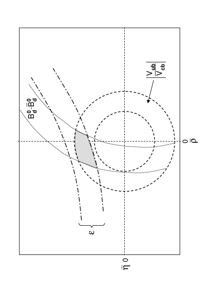
Figure 7: Schematic determination of the Unitarity Triangle.

Step 4:

From the observed $B^{0}_{d}-\bar{B}^{0}_{d}$ mixing parametrized by $\Delta M_{d}$ the side $BA=R_{t}$ of the unitarity triangle can be determined:

$$R_{t}=\frac{1}{\lambda}\frac{|V_{td}|}{|V_{cb}|}=1.0\cdot\left[\frac{|V_{td}|}{8.8\cdot 10^{-3}}\right]\left[\frac{0.040}{|V_{cb}|}\right]$$ (4.83)

with

$$|V_{td}|=8.8\cdot 10^{-3}\left[\frac{200\,{\rm MeV}}{\sqrt{\hat{B}_{B_{d}}}F_{B_{d}}}\right]\left[\frac{170~{}GeV}{\overline{m}_{\rm t}(m_{\rm t})}\right]^{0.76}\left[\frac{\Delta M_{d}}{0.50/{\rm ps}}\right]^{0.5}\sqrt{\frac{0.55}{\eta_{B}}}.$$ (4.84)

Since $m_{\rm t}$, $\Delta M_{d}$ and $\eta_{B}$ are already rather precisely known, the main uncertainty in the determination of $|V_{td}|$ from $B_{d}^{0}-\bar{B}_{d}^{0}$ mixing comes from $F_{B_{d}}\sqrt{\hat{B}_{B_{d}}}$. Note that $R_{t}$ suffers from additional uncertainty in $|V_{cb}|$, which is absent in the determination of $|V_{td}|$ this way. The constraint in the $(\bar{\varrho},\bar{\eta})$ plane coming from this step is illustrated in fig. 7.

Step 5:

The measurement of $B^{0}_{s}-\bar{B}^{0}_{s}$ mixing parametrized by $\Delta M_{s}$ together with $\Delta M_{d}$ allows to determine $R_{t}$ in a different manner. Using (3.60) one finds

$$\frac{|V_{td}|}{|V_{ts}|}=\xi\sqrt{\frac{m_{B_{s}}}{m_{B_{d}}}}\sqrt{\frac{\Delta M_{d}}{\Delta M_{s}}},\qquad\xi=\frac{F_{B_{s}}\sqrt{\hat{B}_{B_{s}}}}{F_{B_{d}}\sqrt{\hat{B}_{B_{d}}}}.$$ (4.85)

Now to an excellent accuracy [27]:

$$|V_{td}|=|V_{cb}|\lambda R_{t},\qquad|V_{ts}|=|V_{cb}|(1-\frac{1}{2}\lambda^{2}+\bar{\varrho}\lambda^{2})~{}.$$ (4.86)

We note next that through the unitarity of the CKM matrix, the present experimental upper bound on $\Delta M_{d}/\Delta M_{s}$ (see table 2) and the value of $|V_{ub}/V_{cb}|$ one has $0\leq\bar{\varrho}\leq 0.5$, where $\xi=1.15\pm 0.06$ [123, 129] has been used. Consequently $|V_{ts}|$ deviates from $|V_{cb}|$ by at most $2\%$. This means that to a very good accuracy we can set $|V_{ts}|=|V_{cb}|$. Consequently (4.85) and the first formula in (4.86) imply

$$R_{t}=0.84~{}\xi_{\rm eff}\sqrt{\frac{\Delta M_{d}}{0.50/ps}},\qquad\xi_{\rm eff}=\xi\sqrt{\frac{15.0/ps}{\Delta M_{s}}}~{}.$$ (4.87)

Using next $\Delta M^{{\rm max}}_{d}=0.50/\mbox{ps}$ one finds a useful formula

$$(R_{t})_{\rm max}=0.84~{}\xi\sqrt{\frac{15.0/ps}{(\Delta M_{s})_{\rm min}}}~{}.$$ (4.88)

If necessary the ${\cal O}(\lambda^{2})$ corrections in (4.86) can be incorporated in (4.87). This will be only required when the error on $\xi$ will be decreased below $2\%$, which is clearly a very difficult task.

One should note that $m_{\rm t}$ and $|V_{cb}|$ dependences have been eliminated this way and that $\xi$ should in principle contain much smaller theoretical uncertainties than the hadronic matrix elements in $\Delta M_{d}$ and $\Delta M_{s}$ separately. The most recent values relevant for (4.88) are summarized in table 2.

Table 2: The ranges of the input parameters.

Quantity	Central	Error
$|V_{cb}|$	0.041	$\pm 0.002$
$|V_{ub}/V_{cb}|$	$0.085$	$\pm 0.018$
$|V_{ub}|$	$0.00349$	$\pm 0.00076$
$\hat{B}_{K}$	0.85	$\pm 0.15$
$\sqrt{\hat{B}_{d}}F_{B_{d}}$	$230\,{\rm MeV}$	$\pm 40\,{\rm MeV}$
$m_{\rm t}$	$166\,{\rm GeV}$	$\pm 5\,{\rm GeV}$
$(\Delta M)_{d}$	$0.487/\mbox{ps}$	$\pm 0.014/\mbox{ps}$
$(\Delta M)_{s}$	$>15.0/\mbox{ps}$
$\xi$	$1.15$	$\pm 0.06$

4.2 Numerical Results

4.2.1 Input Parameters

The input parameters needed to perform the standard analysis of the unitarity triangle are given in table 2. In constructing this table I was guided to a large extent by the reviews [122, 123, 129, 133, 134]. I am aware of the fact that other authors would possibly use slightly different ranges for input parameters. Still table 2 is representative for the present situation. Please note, however, that the error on $|V_{ub}|$ in table 2 is by a factor of two larger than in [123]. I do not think that our present understanding of theoretical uncertainties in the determination of $|V_{ub}|$ is sufficiently good that an error of $\pm 10\%$ on this element can be defended.

The great progress during the last year has been the improved lower limit on $\Delta M_{s}$ from LEP and SLD as reviewed in [133]. The value of $m_{\rm t}$ refers to the running current top quark mass defined at $\mu=m_{\rm t}^{Pole}$. It corresponds to $m_{\rm t}^{Pole}=174.3\pm 5.1\,{\rm GeV}$ measured by CDF and D0 [135].

Figure 8: The Unitarity Triangle as of January 2001.

4.2.2 Various Error Analyses

Having set the input parameters and their uncertainties there is the question how to treat the theoretical uncertainties in a quantitative analysis. There is a hot discussion on this issue, that can be traced by reading [10, 123, 133, 134, 136, 137, 138]. Basically three different approaches can be found in the literature:

• Gaussian Method: The experimentally measured numbers and the theoretical input parameters are used with Gaussian errors. Examples are the analyses in [123, 137, 139]. There are some small differences in the actual treatment of errors in these papers. We refer to [123] for a detailed presentation.

• BaBar $95\%~{}C.L.$ Scanning Method: This method has been developed in [136] and is the official method of the BaBar collaboration [8]. In this method one sets the theoretical input parameters at some fixed values and finds the allowed ($95\%~{}C.L.$) region for $(\bar{\varrho},\bar{\eta})$ by using gaussian errors for the experimental input parameters. Repeating this procedure for different sets of the values of the theoretical input parameters one obtains an envelope of $95\%~{}C.L.$ regions. The latest application of this method can be found in [138].

• Simple Scanning: Both the experimentally measured numbers and the theoretical input parameters are scanned independently within ranges, given for instance in table 2. This is the method used for instance by Rosner [10] and by myself below.

In my opinion the use of Gaussian errors for theoretical input parameters is questionable but I do not want to enter this discussion here. A recent attempt to justify this method can be found in [123, 133]. Yet, when the lattice calculations improve dramatically I could imagine that one could defend this approach. On the other hand the simple scanning method appears to be too conservative. It should be stressed that only the gaussian method pretends to give standard deviations for the output quantities. The scanning methods can only give ranges for the output quantities. The BaBar scanning gives generally the ranges for quantities of interest which are comparable to the ones found by the more naive scanning used here. The $95\%C.L.$ ranges from the gaussian method are not so different from the ones obtained by the scanning methods and consequently global pictures of the unitarity triangle obtained by these methods are compatible with each other. In order to get the full story the interested reader should have a look at [123, 137, 138]. In particular the first paper contains very useful material.

In this section I will present the results of my simple scanning analysis and of a Gaussian analysis by Stefan Schael who used the same input parameters. For the rest of these lectures I will only use simple scanning, except for $\varepsilon^{\prime}/\varepsilon$ where also the results of the Gaussian method will be presented. The quoted results of the scanning method for a quantity $Q$ given below should be understood as follows:

$$\left\{Q=A\pm B\right\}\equiv\left\{A-B\leq Q\leq A+B\right\}$$ (4.89)

This means that the central value $A$ does not generally correspond to central values of the input parameters.

4.2.3 Output of the Standard Analysis

Using simultaneously the five steps discussed above one finds the allowed region of $(\bar{\varrho},\bar{\eta})$. In fig. 8 we show the result of an analysis by Stefan Schael which uses the input parameters of table 2. Only the dark region is allowed. From this figure one extracts

$$\alpha=93^{\circ}\pm 11^{\circ},\qquad\beta={23.6^{\circ}}^{+4.9^{\circ}}_{-4.3^{\circ}},\qquad\gamma=64^{\circ}\pm 11^{\circ},$$ (4.90)

$$\sin 2\beta=0.73^{+0.07}_{-0.14},\qquad|V_{td}|=(8.0\pm 0.7)\cdot 10^{-3}~{}.$$ (4.91)

In this analysis Gaussian errors for all input parameters have been used. My own, more conservative analysis that uses scanning for all input parameters gives

$$78.8^{\circ}\leq\alpha\leq 120^{\circ},\qquad 15.1^{\circ}\leq\beta\leq 28.6^{\circ},\qquad 37.9^{\circ}\leq\gamma\leq 76.5^{\circ}$$ (4.92)

$$\sin 2\beta=0.67\pm 0.17,\qquad|V_{td}|=(8.0\pm 1.3)\cdot 10^{-3}~{}.$$ (4.93)

The ”true” errors are probably between these two estimates. The results of both analyses are summarized in table 3.

Figure 9: Conservative Unitarity Triangle as of January 2001.

The allowed region for $(\bar{\varrho},\bar{\eta})$ resulting from the scanning method is presented in fig. 9. It is the shaded area on the right hand side of the circle representing the lower bound for $(\Delta M)_{s}$, that is $(\Delta M)_{s}>15/ps$. The hyperbolas in fig. 9 give the constraint from $\varepsilon$ and the two circles centered at $(0,0)$ the constraint from $|V_{ub}/V_{cb}|$. The circle on the right comes from $B^{0}_{d}-\bar{B}^{0}_{d}$ mixing and excludes the region to its right. We observe that $B^{0}_{d}-\bar{B}^{0}_{d}$ mixing is almost ineffective for the chosen ranges of the input parameters within the SM and the allowed region is governed by $|V_{ub}/V_{cb}|$, $\Delta M_{s}$ and $\varepsilon$. We also observe that the region $\bar{\varrho}<0$ is practically excluded by the lower bound on $\Delta M_{s}$. It is clear from this figure that $(\Delta M)_{s}$ is a very important ingredient in this analysis and that the measurement of $(\Delta M)_{s}$ giving also lower bound on $R_{t}$ will have a large impact on the plots in figs. 8 and 9. Finally we find that whereas the angle $\beta$ is rather constrained, the uncertainties in $\alpha$ and $\gamma$ are substantially larger.

Table 3: Output of the Standard Analysis. $\lambda_{t}=V^{*}_{ts}V_{td}$.

Quantity	Scanning	Gaussian
$\mid V_{td}\mid/10^{-3}$	$6.7-9.3$	$8.0\pm 0.7$
$\mid V_{ts}/V_{cb}\mid$	$0.979-0.993$	$0.984\pm 0.004$
$\mid V_{td}/V_{ts}\mid$	$0.16-0.22$	$0.20\pm 0.02$
$\sin(2\beta)$	$0.50-0.84$	$0.73^{+0.07}_{-0.14}$
$\sin(2\alpha)$	$-0.87-0.38$	$-0.1\pm 0.3$
$\sin(\gamma)$	$0.61-0.97$	$0.9\pm 0.1$
${\rm Im}\lambda_{t}/10^{-4}$	$0.94-1.60$	$1.2\pm 0.2$
$\bar{\eta}$	$0.22-0.46$	$0.36\pm 0.07$
$\bar{\varrho}$	$0.06-0.34$	$0.18\pm 0.09$

4.2.4 An Upper Bound on $\Delta M_{s}$

In view of the expected measurement of $\Delta M_{s}$ in 2001 at Tevatron it is of interest to find its upper bound within the SM. The most straightforward manner to obtain this bound is to set $|V_{ts}|_{max}=0.043$, $\overline{m_{\rm t}}(m_{\rm t})_{max}=171\,{\rm GeV}$ and $(\sqrt{\hat{B}_{B_{s}}}F_{B_{s}})_{max}=300~{}\,{\rm MeV}$ [123, 129] in (3.62). We find

$$\Delta M_{s}<27.5/ps$$ (4.94)

with 16.0/ps obtained for central values of the input parameters.

4.3 First Conclusions

In this section we have completed the determination of the CKM matrix. It is given by the values of $|V_{us}|$, $|V_{cb}|$ and $|V_{ub}|$ in (1.38) and (1.39), the results in table 3 and the unitarity triangle shown in figs. 8 and 9. We should stress, that soon this analysis will be improved through the new information on the angle $\beta$ coming from B factories and Tevatron and on $\Delta M_{s}$ from Tevatron. In particular the latter measurement should have an important impact on the allowed area in the $(\bar{\varrho},\bar{\eta})$ plane.

We conclude that the SM is capable of describing the observed indirect CP violation in $K_{L}$ decays, taking into account the data on $B^{0}_{d,s}-\bar{B}^{0}_{d,s}$ mixings, $|V_{cb}|$ and $|V_{ub}/V_{cb}|$. We also observe that $R_{b}$ and $R_{t}$ from $|V_{ub}/V_{cb}|$ and $B^{0}_{d,s}-\bar{B}^{0}_{d,s}$ mixings alone satisfy the condition (1.36). Taking $(R_{b})_{min}=0.30$, this condition reads $0.70<R_{t}<1.30$. From (4.88) and the lower bound on $\Delta M_{s}$ one has $R_{t}<1.01$. On the other hand $|V_{td}|_{min}$ is governed by $B_{d}^{0}-\bar{B}_{d}^{0}$ mixing. From (4.83) and (4.93) one has then $R_{t}>0.71$. Consequently CP violation in B-decays is predicted on the basis of $|V_{ub}/V_{cb}|$ and $B^{0}_{d,s}-\bar{B}^{0}_{d,s}$ mixings alone, even if our conservative analysis does not show this so clearly. Indeed the first result for the CP asymmetry in $B_{d}\to\psi K_{S}$ with $\sin 2\beta=0.79\pm 0.42$ from CDF [140], presented in 1999, established CP violation in B decays at $93\%$ C.L. and moreover was consistent with (4.91) and (4.93). Yet the reality could turn out to be different as we will see in a moment.

4.4 First Results on $\sin 2\beta$ from B Factories

Since the summer 2000 we have the first results on the time dependent CP asymmetry, $a_{\psi K_{S}}$, from BaBar [141] and Belle [142]. These results indicate that the value of the angle $\beta$ in the unitarity triangle could turn out to be substantially smaller than expected on the basis of the standard analysis of the unitarity triangle within the SM presented above. Indeed the three measurements of this asymmetry

$$(\sin 2\beta)_{\psi K_{S}}=\left\{\begin{array}[]{ll}0.79\pm 0.42&{\rm(CDF)}~{}\cite[cite]{[\@@bibref{}{CDFB}{}{}]}\\ 0.12\pm 0.37\pm 0.09&{\rm(BaBar)}~{}\cite[cite]{[\@@bibref{}{BaBar}{}{}]}\\ 0.45\pm 0.44\pm 0.08&{\rm(Belle)}~{}\cite[cite]{[\@@bibref{}{Belle}{}{}]}\end{array}\right.$$ (4.95)

imply the grand average

$$(\sin 2\beta)_{\psi K_{S}}=0.42\pm 0.24~{}.$$ (4.96)

This should be compared with the results of the standard analysis of the unitarity triangle within the SM presented above which gave $\sin 2\beta=0.73^{+0.07}_{-0.14}$ and $\sin 2\beta=0.67\pm 0.17$ for the gaussian and scanning analyses respectively. Similar values can be found in the literature

$$(\sin 2\beta)_{SM}=\left\{\begin{array}[]{ll}0.69\pm 0.07&~{}\cite[cite]{[\@@bibref{}{Football}{}{}]}\\ 0.70\pm 0.24&~{}\cite[cite]{[\@@bibref{}{ALI00}{}{}]}\\ 0.63\pm 0.12&~{}\cite[cite]{[\@@bibref{}{SCHUNE}{}{}]}\end{array}\right.$$ (4.97)

where the last two results represent $95\%$ C.L. ranges. Clearly in view of the large spread of experimental results and large statistical errors in (4.95), the SM estimates in (4.91), (4.93) and (4.97) are compatible with the experimental value of $(\sin 2\beta)_{\psi K_{S}}$ in (4.96). Yet the small values of $\sin 2\beta$ found by BaBar and Belle may give some hints for new physics contributions to $B^{0}_{d}-\bar{B}^{0}_{d}$ and $K^{0}-\bar{K}^{0}$ mixings. In particular as discussed recently in several papers [143]-[146] new CP violating phases in $B^{0}_{d}-\bar{B}^{0}_{d}$ and $K^{0}-\bar{K}^{0}$ mixing could be responsible for small values of $\sin 2\beta$ in (4.96). In this context an absolut lower bound on $\sin 2\beta$ in models with minimal flavour violation has been derived in [147]. We will discuss this bound and its update in detail in Section 9. Finally a general model independent analysis of new physics in $B^{\pm}\to\psi K^{\pm}$ and $B^{0}_{d}\to\psi K_{S}$ has been presented very recently in [148].

On the other hand as stressed in [143] the SM estimates of $\sin 2\beta$ are sensitive to the assumed ranges for the parameters

$$|V_{cb}|,\quad|V_{ub}/V_{cb}|,\quad\hat{B}_{K},\quad\sqrt{\hat{B}_{d}}F_{B_{d}},\quad\xi~{},$$ (4.98)

that enter the standard analysis of the unitarity triangle. While for “reasonable ranges” (see table 2) of these parameters, values of $\sin 2\beta\leq 0.5$ are essentially excluded, such low values within the SM could still be possible if some of the parameters in (4.98) were chosen outside these ranges. In particular for $|V_{ub}/V_{cb}|\leq 0.06$ or $\hat{B}_{K}\geq 1.3$ or $\xi\geq 1.4$ the value for $\sin 2\beta$ lower than 0.5 could be obtained within the SM. We agree with these findings.

In what follows we will assume the ”reasonable ranges” for the parameters as given in table 2 and we will use the values of the CKM parameters determined in this section to predict various branching ratios for rare and CP-violating decays. This means we will not take into account in our numerical analyses the recent results from BaBar and Belle. We will return to them in Section 9 where some aspects of the physics beyond the SM will be discussed. Thus the next four sections apply only to the SM and could be affected considerably if the improved measurements of the asymmetry $a_{\psi K_{S}}$ by BaBar, Belle, CDF and D0 will confirm with higher precision the present low values of $\sin 2\beta$ from BaBar and Belle. This would be truely exciting!

5 $\varepsilon^{\prime}/\varepsilon$ in the Standard Model

5.1 Preliminaries

Direct CP violation remains one of the important targets of contemporary particle physics [149]. In the case of $K\to\pi\pi$, a non-vanishing value of the ratio Re($\varepsilon^{\prime}/\varepsilon$) would give the first signal for direct CP violation ruling out superweak models [150] in which $\varepsilon^{\prime}/\varepsilon=0$. Until February 1999 the experimental situation on $\varepsilon^{\prime}/\varepsilon$ was rather unclear:

$${\rm Re}(\varepsilon^{\prime}/\varepsilon)=\left\{\begin{array}[]{ll}(23\pm 7)\cdot 10^{-4}&{\rm(NA31)}~{}\cite[cite]{[\@@bibref{}{barr:93}{}{}]}~{},\\ (7.4\pm 5.9)\cdot 10^{-4}&{\rm(E731)}~{}\cite[cite]{[\@@bibref{}{gibbons:93}{}{}]}.\end{array}\right.$$ (5.1)

While the result of the NA31 collaboration at CERN [151] clearly indicated direct CP violation, the value of E731 at Fermilab [152], was compatible with superweak theories. This controversy is now settled in favour of NA31. The most recent experimental results for the ratio $\varepsilon^{\prime}/\varepsilon$ from Fermilab and CERN presented during 1999 and 2000 read

$${\rm Re}(\varepsilon^{\prime}/\varepsilon)=\left\{\begin{array}[]{ll}(28.0\pm 4.1)\cdot 10^{-4}&{\rm(KTeV)}~{}\cite[cite]{[\@@bibref{}{KTEV}{}{}]}~{},\\ (14.0\pm 4.3)\cdot 10^{-4}&{\rm(NA48)}~{}\cite[cite]{[\@@bibref{}{NA48}{}{}]}~{}.\end{array}\right.$$ (5.2)

Together with the NA31 measurement these data confidently establish direct CP violation in nature and taking also the E731 result into account one finds the grand average [154]

$${\rm Re}(\varepsilon^{\prime}/\varepsilon)=(19.2\pm 2.4)\cdot 10^{-4}~{},$$ (5.3)

close to the NA31 result.

While the experimentalists should be congratulated for these results, the situation is clearly unsatisfactory. The KTeV result is by a factor of four larger than the E731 result. In addition the substantial difference between KTeV and NA48 results is disturbing. Let us hope that these issues will be clarified soon. In this context an independent measurement of $\varepsilon^{\prime}/\varepsilon$ by KLOE at Frascati, which uses a different experimental technique than KTeV and NA48 will be very important.

There is a long history of calculations of $\varepsilon^{\prime}/\varepsilon$ in the SM beginning with the pioneering calculations in [155] and [156] and the first extensive phenomenological analyses in [157]. Over the 1980’s these calculations were refined through the inclusion of QED penguin effects for $m_{\rm t}\ll M_{\rm W}$ [158, 159, 160], the inclusion of isospin breaking in the quark masses [159, 160, 161], through improved estimates of hadronic matrix elements in the framework of the $1/N$ approach [162] and the inclusion of QCD penguins, electroweak penguins ($\gamma$ and $Z^{0}$ penguins) and the relevant box diagrams for arbitrary top quark mass [163, 164]. The strong cancellation between QCD penguins and electroweak penguins for $m_{t}>150~{}\,{\rm GeV}$ found in these two papers was confirmed by other authors [165].

During the 1990’s considerable progress has been made by calculating complete NLO corrections to $\varepsilon^{\prime}$ [40]–[44]. Together with the NLO corrections to $\varepsilon$ and $B^{0}-\bar{B}^{0}$ mixing [51, 52, 54], this allowed a complete NLO analysis of $\varepsilon^{\prime}/\varepsilon$ including constraints from the observed indirect CP violation ($\varepsilon$) and $B_{d,s}^{0}-\bar{B}_{d,s}^{0}$ mixings ($\Delta M_{d,s}$). The improved determination of the $V_{ub}$ and $V_{cb}$ elements of the CKM matrix and in particular the determination of the top quark mass $m_{\rm t}$ had of course also an important impact on $\varepsilon^{\prime}/\varepsilon$.

While until 1999 only a few groups were involved in detailed analyses of $\varepsilon^{\prime}/\varepsilon$ [42],[163]-[169], the new results from KTeV and NA48 prompted a number of theorists to join the efforts to calculate this important ratio. By the end of 2000 the theoretical $\varepsilon^{\prime}/\varepsilon$-club has more than 30 members.

The developments of the last two years include new estimates of hadronic matrix elements using lattice simulations [122], various versions of the large–N approach, chiral quark model, QCD sum rules and other approches mentioned below. Simultaneously extensive studies of final state interactions (FSI), isospin breaking effects and electromagnetic effects in $\varepsilon^{\prime}/\varepsilon$ have been pursued. Finally the impact of new physics on $\varepsilon^{\prime}/\varepsilon$ has been analyzed in various extentions of the SM.

We will briefly review these topics below. To this end we have to recall a number of useful formulae for $\varepsilon^{\prime}/\varepsilon$. Other reviews of $\varepsilon^{\prime}/\varepsilon$ can be found in [169]-[172]

5.2 Basic Formulae

The parameter $\varepsilon^{\prime}$ is given in terms of the isospin amplitudes $A_{I}$ in (3.26). Applying OPE to these amplitudes one finds [42, 167]

$$\frac{\varepsilon^{\prime}}{\varepsilon}={\rm Im}\lambda_{t}\cdot F_{\varepsilon^{\prime}},$$ (5.4)

where

$$F_{\varepsilon^{\prime}}=\left[P^{(1/2)}-P^{(3/2)}\right]\exp(i\Phi),$$ (5.5)

with

$$P^{(1/2)} = r\sum y_{i}\langle Q_{i}\rangle_{0}(1-\Omega_{\rm IB})~{},$$ (5.6)

$$P^{(3/2)} = \frac{r}{\omega}\sum y_{i}\langle Q_{i}\rangle_{2}~{}.~{}~{}~{}~{}~{}~{}$$ (5.7)

Here

$$r=\frac{G_{\rm F}\omega}{2|\varepsilon|{\rm Re}A_{0}}~{},\qquad\langle Q_{i}\rangle_{I}\equiv\langle(\pi\pi)_{I}|Q_{i}|K\rangle~{},\qquad\omega=\frac{{\rm Re}A_{2}}{{\rm Re}A_{0}}.$$ (5.8)

Since

$$\Phi=\Phi_{\varepsilon^{\prime}}-\Phi_{\varepsilon}\approx 0,$$ (5.9)

$F_{\varepsilon^{\prime}}$ and $\varepsilon^{\prime}/\varepsilon$ are real to an excellent approximation. The operators $Q_{i}$ have been given already in (2.4)-(2.8). The Wilson coefficient functions $y_{i}(\mu)$ were calculated including the complete next-to-leading order (NLO) corrections in [40]–[44]. The details of these calculations can be found there and in the review [3]. Their numerical values for $\Lambda_{\overline{\rm MS}}^{(4)}$ corresponding to $\alpha_{\overline{MS}}^{(5)}(M_{\rm Z})=0.119\pm 0.003$ and two renormalization schemes (NDR and HV) are given in table 4 [173].

Table 4: $\Delta S=1$ Wilson coefficients at $\mu=m_{\rm c}=1.3\,{\rm GeV}$ for $m_{\rm t}=165\,{\rm GeV}$ and $f=3$ effective flavours. $y_{1}=y_{2}\equiv 0$.

	$\Lambda_{\overline{\rm MS}}^{(4)}=290\,{\rm MeV}$		$\Lambda_{\overline{\rm MS}}^{(4)}=340\,{\rm MeV}$		$\Lambda_{\overline{\rm MS}}^{(4)}=390\,{\rm MeV}$
Scheme	NDR	HV	NDR	HV	NDR	HV
$y_{3}$	0.027	0.030	0.030	0.034	0.033	0.038
$y_{4}$	–0.054	–0.056	–0.059	–0.061	–0.064	–0.067
$y_{5}$	0.006	0.015	0.005	0.016	0.003	0.017
$y_{6}$	–0.082	–0.074	–0.092	–0.083	–0.105	–0.093
$y_{7}/\alpha$	–0.038	–0.037	–0.037	–0.036	–0.037	–0.034
$y_{8}/\alpha$	0.118	0.127	0.134	0.143	0.152	0.161
$y_{9}/\alpha$	–1.410	–1.410	–1.437	–1.437	–1.466	–1.466
$y_{10}/\alpha$	0.496	0.502	0.539	0.546	0.585	0.593

It is customary in phenomenological applications to take ${\rm Re}A_{0}$ and $\omega$ from experiment, i.e.

$${\rm Re}A_{0}=3.33\cdot 10^{-7}\,{\rm GeV},\qquad\omega=\frac{{\rm Re}A_{2}}{{\rm Re}A_{0}}=0.045,$$ (5.10)

where the last relation reflects the so-called $\Delta I=1/2$ rule. This strategy avoids to a large extent the hadronic uncertainties in the real parts of the isospin amplitudes $A_{I}$.

The sum in (5.6) and (5.7) runs over all contributing operators. $P^{(3/2)}$ is fully dominated by electroweak penguin contributions. $P^{(1/2)}$ on the other hand is governed by QCD penguin contributions which are suppressed by isospin breaking in the quark masses ($m_{u}\not=m_{d}$). The latter effect is described by

$$\Omega_{\rm IB}=\frac{1}{\omega}\frac{({\rm Im}A_{2})_{\rm IB}}{{\rm Im}A_{0}}\,.$$ (5.11)

The main source of uncertainty in the calculation of $\varepsilon^{\prime}/\varepsilon$ are the hadronic matrix elements $\langle Q_{i}\rangle_{I}$ and $\Omega_{\rm IB}$ as we will see later on. $\langle Q_{i}\rangle_{I}$ generally depend on the renormalization scale $\mu$ and on the scheme used to renormalize the operators $Q_{i}$. These two dependences are canceled by those present in the Wilson coefficients $y_{i}(\mu)$ so that the resulting physical $\varepsilon^{\prime}/\varepsilon$ does not (in principle) depend on $\mu$ and on the renormalization scheme for the operators. Unfortunately, the accuracy of the present non-perturbative methods used to evalutate $\langle Q_{i}\rangle_{I}$ is not sufficient to have the $\mu$ and scheme dependences of $\langle Q_{i}\rangle_{I}$ fully under control. We believe that this situation will change once the lattice calculations improve. A brief review of the existing methods including most recent developments will be given below.

5.3 An Analytic Formula for $\varepsilon^{\prime}/\varepsilon$

The basic formulae for $\varepsilon^{\prime}/\varepsilon$ presented above are not very transparent and we would like to improve on this. To this end let us first determine as many matrix elements $\langle Q_{i}\rangle_{I}$ as possible from the leading CP conserving $K\to\pi\pi$ decays, for which the experimental data is summarized in (5.10). This determination is particularly easy if one sets $\mu=m_{c}$ [42]. The details of this approach will not be discussed here. It sufficies to say that this method allows to determine only the matrix elements of the $(V-A)\otimes(V-A)$ operators. Explicit formulae can be found in [42]. For the central value of ${\rm Im}\lambda_{t}$ these operators give a negative contribution to $\varepsilon^{\prime}/\varepsilon$ of about $-2.5\cdot 10^{-4}$. This shows that they are only relevant if $\varepsilon^{\prime}/\varepsilon$ is below $1\cdot 10^{-3}$.

Unfortunately the method in [42] does not provide the matrix elements of the dominant $(V-A)\otimes(V+A)$ operators and one has to use non-perturbative methods to estimate them. In this context the calculations of Bertolini and collaborators [169] within the chiral quark model should be mentioned. These authors have determined the parameters of this model by taking the constraints (5.10) into account. In this manner they were able to determine not only the matrix elements of the $(V-A)\otimes(V-A)$ operators, as in [42], but also the matrix elements of the $(V-A)\otimes(V+A)$ operators. This is clearly interesting. On the other hand, it is not clear how well the chiral quark model approximates QCD and consequently whether the extracted values of the relevant matrix elements have anything to do with the true QCD values. For this reason we will not use them here.

In order to exhibit the matrix elements of the dominant $(V-A)\otimes(V+A)$ operators in an analytic formula for $\varepsilon^{\prime}/\varepsilon$, we first express them in terms of non-perturbative parameters $B_{i}^{(1/2)}$ and $B_{i}^{(3/2)}$ as follows:

$$\langle Q_{i}\rangle_{0}\equiv B_{i}^{(1/2)}\,\langle Q_{i}\rangle_{0}^{\rm(vac)}\,,\qquad\langle Q_{i}\rangle_{2}\equiv B_{i}^{(3/2)}\,\langle Q_{i}\rangle_{2}^{\rm(vac)}\,.$$ (5.12)

The label “vac” stands for the vacuum insertion estimate of the hadronic matrix elements in question for which $B_{i}^{(1/2)}=B_{i}^{(3/2)}=1$.

The Wilson coefficients $y_{5}$, $y_{7}$ and $y_{8}$ are much smaller than $y_{6}$. On the other hand the contributions of $\langle Q_{7,8}\rangle_{2}$ are enhanced by the factor $1/\omega\approx 22$ as seen in (5.7). But $y_{7}$ is substantially smaller than $y_{8}$ and $\langle Q_{7}\rangle_{0,2}$ are colour suppressed. It is then not surprising [42] that $\varepsilon^{\prime}/\varepsilon$ is only weakly sensitive to the values of the parameters $B_{5}^{(1/2)}$, $B_{7}^{(1/2)}$, $B_{8}^{(1/2)}$ and $B_{7}^{(3/2)}$ as long as their absolute values are not substantially larger than 1. On the basis of existing non-perturbative approaches we can assume that this is indeed the case.

Following [42] we set then

$$B_{7,8}^{(1/2)}(m_{\rm c})=1,\qquad B_{5}^{(1/2)}(m_{\rm c})=B_{6}^{(1/2)}(m_{\rm c})\equiv B_{6}^{(1/2)},\qquad B_{7}^{(3/2)}(m_{\rm c})=B_{8}^{(3/2)}(m_{\rm c})\equiv B_{8}^{(3/2)}~{}.$$ (5.13)

This strategy [42] allows then to express $\varepsilon^{\prime}/\varepsilon$ or equivalently $F_{\varepsilon^{\prime}}$ in terms of of the following parameters

$$B_{6}^{(1/2)},\qquad B_{8}^{(3/2)},\qquad\Omega_{\rm IB},\qquad m_{\rm s},\qquad m_{\rm t},\qquad\Lambda_{\overline{\rm MS}}^{(4)}~{}.$$ (5.14)

The appearence of $m_{\rm s}$ originates in

$$\langle Q_{6}\rangle_{0}^{\rm(vac)}\sim 1/m_{\rm s}^{2}(\mu),\qquad\langle Q_{8}\rangle_{2}^{\rm(vac)}\sim 1/m_{\rm s}^{2}(\mu)~{}.$$ (5.15)

$\Lambda_{\overline{\rm MS}}^{(4)}$ and $m_{\rm t}$ enter through the coefficients $y_{i}$.

With all this information at hand, it is possible [167, 174] to cast the formal expressions for $\varepsilon^{\prime}/\varepsilon$ in (5.4)–(5.7) into an analytic formula which exhibits the dependence on the parameters in (5.14). We set $\Omega_{\rm IB}=0.16$ for the moment. We will return to it below. The analytic formula given below, while being rather accurate, exhibits various features which are not transparent in a pure numerical analysis. It can be used in phenomenological applications if one is satisfied with a few percent accuracy. Needless to say, in the numerical analysis [173, 109] presented below we have used exact expressions.

In this formulation the function $F_{\varepsilon^{\prime}}$ is given simply as follows:

$$F_{\varepsilon^{\prime}}=P_{0}+P_{X}\,X_{0}(x_{t})+P_{Y}\,Y_{0}(x_{t})+P_{Z}\,Z_{0}(x_{t})+P_{E}\,E_{0}(x_{t})$$ (5.16)

with the $m_{\rm t}$-dependent functions given in subsection 2.6.

The coefficients $P_{i}$ are given in terms of $B_{6}^{(1/2)}$, $B_{8}^{(3/2)}$ and $m_{\rm s}(m_{\rm c})$ as follows:

$$P_{i}=r_{i}^{(0)}+r_{i}^{(6)}R_{6}+r_{i}^{(8)}R_{8}\,$$ (5.17)

where

$$R_{6}\equiv B_{6}^{(1/2)}\left[\frac{137\,{\rm MeV}}{m_{\rm s}(m_{\rm c})+m_{\rm d}(m_{\rm c})}\right]^{2},\qquad R_{8}\equiv B_{8}^{(3/2)}\left[\frac{137\,{\rm MeV}}{m_{\rm s}(m_{\rm c})+m_{\rm d}(m_{\rm c})}\right]^{2}.$$ (5.18)

The $P_{i}$ are renormalization scale and scheme independent. They depend, however, on $\Lambda_{\overline{\rm MS}}^{(4)}$. In table 5 we give the numerical values of $r_{i}^{(0)}$, $r_{i}^{(6)}$ and $r_{i}^{(8)}$ for different values of $\Lambda_{\overline{\rm MS}}^{(4)}$ at $\mu=m_{\rm c}$ in the NDR renormalization scheme [109]. Actually at NLO only $r_{0}$ coefficients are renormalization scheme dependent. The last row gives them in the HV scheme. The inspection of table 5 shows that the terms involving $r_{0}^{(6)}$ and $r_{Z}^{(8)}$ dominate the ratio $\varepsilon^{\prime}/\varepsilon$. Moreover, the function $Z_{0}(x_{t})$ representing a gauge invariant combination of $Z^{0}$- and $\gamma$-penguins grows rapidly with $m_{\rm t}$ and due to $r_{Z}^{(8)}<0$ these contributions suppress $\varepsilon^{\prime}/\varepsilon$ strongly for large $m_{\rm t}$ [163, 164].

Table 5: Coefficients in the formula (5.17) for various $\Lambda_{\overline{\rm MS}}^{(4)}$ in the NDR scheme. The last row gives the $r_{0}$ coefficients in the HV scheme.

	$\Lambda_{\overline{\rm MS}}^{(4)}=290\,{\rm MeV}$			$\Lambda_{\overline{\rm MS}}^{(4)}=340\,{\rm MeV}$			$\Lambda_{\overline{\rm MS}}^{(4)}=390\,{\rm MeV}$
$i$	$r_{i}^{(0)}$	$r_{i}^{(6)}$	$r_{i}^{(8)}$	$r_{i}^{(0)}$	$r_{i}^{(6)}$	$r_{i}^{(8)}$	$r_{i}^{(0)}$	$r_{i}^{(6)}$	$r_{i}^{(8)}$
0	–3.122	10.905	1.423	–3.167	12.409	1.262	–3.210	14.152	1.076
$X$	0.556	0.019	0	0.540	0.023	0	0.526	0.027	0
$Y$	0.404	0.080	0	0.387	0.088	0	0.371	0.097	0
$Z$	0.412	–0.015	–9.363	0.474	–0.017	–10.186	0.542	–0.019	–11.115
$E$	0.204	–1.276	0.409	0.188	–1.399	0.459	0.172	–1.533	0.515
0	–3.097	9.586	1.045	–3.141	10.748	0.867	–3.183	12.058	0.666

Finally by investigating numerically the formula (5.16) it is possible to find a crude approximation for $F_{\varepsilon^{\prime}}$:

$$F_{\varepsilon^{\prime}}\approx 13\cdot\left[\frac{110\,{\rm MeV}}{m_{\rm s}(2~{}\,{\rm GeV})}\right]^{2}\left[B_{6}^{(1/2)}(1-\Omega_{\rm IB})-0.4\cdot B_{8}^{(3/2)}\left(\frac{m_{\rm t}}{165\,{\rm GeV}}\right)^{2.5}\right]\left(\frac{\Lambda_{\overline{\rm MS}}^{(4)}}{340~{}\,{\rm MeV}}\right)~{}.$$ (5.19)

This formula while exhibiting very transparently the dependence of $\varepsilon^{\prime}/\varepsilon$ on the parameters (5.14) should not be used for any serious numerical analysis.

We observe the known features:

• $F_{\varepsilon^{\prime}}$ increases with increasing $\Lambda_{\overline{\rm MS}}^{(4)}$. In fact the renormalization group effects play an important role here. If one did not include them $\varepsilon^{\prime}/\varepsilon$ would be typically ${\cal O}(10^{-5})$. On the other hand the formula (5.19) is only valid for $\Lambda_{\overline{\rm MS}}^{(4)}>200\,{\rm MeV}$. $F_{\varepsilon^{\prime}}$ does not vanish for $\Lambda_{\overline{\rm MS}}^{(4)}=0$.

• $F_{\varepsilon^{\prime}}$ increases with increasing $B_{6}^{(1/2)}$ that represents QCD penguins. It decreases with increasing $B_{8}^{(3/2)}$ that represents electroweak penguins. The latter contribution increases with increasing $m_{\rm t}$.

• The partial cancellation between QCD penguin ($B_{6}^{(1/2)}$) and electroweak penguin ($B_{8}^{(3/2)}$) contributions requires accurate values of $B_{6}^{(1/2)}$ and $B_{8}^{(3/2)}$ for an acceptable estimate of $\varepsilon^{\prime}/\varepsilon$. Because of the accurate value $m_{\rm t}(m_{\rm t})=166\pm 5~{}\,{\rm GeV}$, the uncertainty in $\varepsilon^{\prime}/\varepsilon$ due to the top quark mass amounts only to a few percent.

• The $1/m_{\rm s}^{2}$ dependence is an artifact of the decomposition of the matrix elements into $B_{i}$–factors and the vacuum insertion matrix elements as given in (5.12). We will return to this point below.

5.4 The Status of $m_{\rm s}$, $B_{6}^{(1/2)}$, $B_{8}^{(3/2)}$, $\Omega_{\rm IB}$ and $\Lambda_{\overline{\rm MS}}^{(4)}$

5.4.1 $m_{\rm s}$

The most recent values for $m_{\rm s}(2\,{\rm GeV})$ extracted from lattice calculations, QCD sum rules and $\tau$–decays are summarized in table 6. The lattice result is the most recent “world average” of Lubicz [175]. See also [180]. It is higher than the older result from Gupta [181] but could decrease a bit when the calculations with dynamical fermions are completed. Significant progress has been made in the last two years by the introduction of improved actions and non-perturbative renormalization techniques. Quenched calculations give $m_{\rm s}(2\,{\rm GeV})=(110\pm 15)~{}\,{\rm MeV}$ and the increased error in table 6 gives the estimate of the quenching error based on the ca culations with two flavours. Details with references to calculations of different groups can be found in [175]. The recent QCD sum rule values are considerably smaller than the older ones [182]. The same comment applies to $m_{\rm s}$ from $\tau$–decays.

While the situation regarding $m_{\rm s}$ improved considerably during the last two years and the values obtained using different methods are coming closer to each other, the error on $m_{\rm s}$ is still large. In our numerical analysis of $\varepsilon^{\prime}/\varepsilon$ we will use

$$m_{\rm s}(\mu)=\left\{\begin{array}[]{ll}(110\pm 20)\;\,{\rm MeV}&\mu=2\,{\rm GeV}\\ (130\pm 25)\;\,{\rm MeV}&\mu=m_{\rm c}\end{array}\right.$$ (5.20)

which is in the ball park of the results given in table 6. Here $m_{\rm c}=1.3\,{\rm GeV}$.

Five years ago values like $m_{\rm s}(2\,{\rm GeV})=130-150\,{\rm MeV}$ could be found in the literature. Beginning with the work of Gupta [181] the values of $m_{\rm s}$ decreased considerably, which makes the values of $\varepsilon^{\prime}/\varepsilon$ larger. On the other hand QCD sum rules allow to derive lower bounds on the strange quark mass. It is found that generally $m_{\rm s}(2\,{\rm GeV})~{}{}_{\textstyle\sim}^{\textstyle>}~{}100\,\,{\rm MeV}$ [183]. We observe that lattice results are very close to this bound.

Table 6: $m_{\rm s}(2\,{\rm GeV})$ obtained using various methods.

Method	$m_{\rm s}(2\,{\rm GeV})~{}[\,{\rm MeV}]$	Reference
Lattice	$110\pm 25$	Lubicz [175]
QCDS	$119\pm 12$	Narison[176]
QCDS	$116\pm 22$	Jamin [177]
QCDS	$115\pm 8$	Maltman [178]
$\tau$–Decays	$114\pm 23$	Pich-Prades [179]

The large sensitivity of $\varepsilon^{\prime}/\varepsilon$ to $m_{\rm s}$ has been known since the analyses in the 1980’s. In the context of the KTeV result this issue has been analyzed in [184]. It has been found that provided $2B_{6}^{(1/2)}-B_{8}^{(3/2)}\leq 2$ the consistency of the SM with the KTeV result requires the $2\sigma$ bound $m_{\rm s}(2\,{\rm GeV})\leq 110\,{\rm MeV}$. Our analysis below is compatible with these findings.

On the other hand, it has been emphasized by Guido Martinelli, Eduardo de Rafael and other researchers in the field that the study of $\varepsilon^{\prime}/\varepsilon$ as a function of $m_{\rm s}$, independently of $B_{6}^{(1/2)}$ and $B_{8}^{(3/2)}$, could be misleading. Indeed a correlation could exist between $m_{\rm s}$ and the latter parameters. In the large–N approach of [162, 185] such correlation is not observed. However, I can imagine that in an approach, like lattice simulations, that calculates the hadronic matrix elements directly, without parametrizing them in terms of $m_{\rm s}$ and $B_{i}$–factors, some correlations in values of these parameters could certainly be present. It will be interesting to study this issue once the lattice calculations improve.

From my point of view, the strange quark mass must be somehow related to the matrix elements $\langle Q_{6}\rangle_{0}$ and $\langle Q_{8}\rangle_{2}$. Afterall $Q_{6}$ and $Q_{8}$ are density-density operators and in the large–N limit the anomalous dimensions of these operators are equal to $-2\gamma_{m}$, where $\gamma_{m}$ is the anomalous dimension of the mass operator [160]. Consequently the $\mu$-dependence of $\langle Q_{6}\rangle_{0}$ and $\langle Q_{8}\rangle_{2}$ is governed to a very good approximation by the $\mu$-dependence of $m_{\rm s}(\mu)$ as shown in (5.15). This has been verified numerically beyond the large–N limit in [42]. This implies that $B_{6}^{(1/2)}$ and $B_{8}^{(3/2)}$ are practically $\mu$-independent and from the point of view of the $\mu$-dependence $m_{\rm s}$ is indeed uncorrelated with $B_{6}^{(1/2)}$ and $B_{8}^{(3/2)}$. On the other hand I can imagine that at fixed $\mu$, there is some correlation between the actual values of $m_{\rm s}$, $B_{6}^{(1/2)}$ and $B_{8}^{(3/2)}$.

In this context it should be recalled [160] that the $\mu$-dependence of $\langle Q_{6}\rangle_{0}$ and $\langle Q_{8}\rangle_{2}$, just discussed, is to a very good approximation canceled by the $\mu$-dependence of $y_{6}(\mu)$ and $y_{8}(\mu)$ respectively. This means that the unphysical $\mu$-dependence in $\varepsilon^{\prime}/\varepsilon$ is very small already in the present calculations. This is a nice feature, which can be seen explicitly within the lare–N approach.

5.4.2 $B_{6}^{(1/2)}$ and $B_{8}^{(3/2)}$

The values for $B_{6}^{(1/2)}$ and $B_{8}^{(3/2)}$ obtained in various approaches are collected in table 7. The lattice results have been obtained at $\mu=2\,{\rm GeV}$. The results in the large–N approach and the chiral quark model correspond to scales below $1\,{\rm GeV}$. However, as explained above, $B_{6}^{(1/2)}$ and $B_{8}^{(3/2)}$ are only weakly dependent on $\mu$. Consequently the comparison of these parameters obtained in different approaches at different $\mu$ is meaningful as long as $\mu>0.8~{}\,{\rm GeV}$.

Next, the values coming from lattice and chiral quark model are given in the NDR renormalization scheme. The corresponding values in the HV scheme can be found using approximate relations [173]

$$(B_{6}^{(1/2)})_{\rm HV}\approx 1.2(B_{6}^{(1/2)})_{\rm NDR},\qquad(B_{8}^{(3/2)})_{\rm HV}\approx 1.2(B_{8}^{(3/2)})_{\rm NDR}.$$ (5.21)

The scheme dependence of these parameters in the large-N approach are to my knowledge not yet under full control but some progress is being made [128, 190, 192].

Concerning the lattice results for $B^{(1/2)}_{6}$, the old results read $B^{(1/2)}_{5,6}(2~{}\,{\rm GeV})=1.0\pm 0.2$ [193, 194]. However, over the last years it has been realized beginning with [195] that lattice calculations of $B_{6}^{(1/2)}$ are very uncertain. One has to conclude that there are no solid predictions for $B^{(1/2)}_{6}$ from the lattice at present. There is a hope that soon results using domain wall fermions not only for $B_{6}^{(1/2)}$ and $B_{8}^{(3/2)}$ but for all hadronic matrix elements entering $\varepsilon^{\prime}/\varepsilon$ will be available. A very informative and critical review of the present situation has been given recently by Laurent Lellouch [122].

The result for $B_{8}^{(3/2)}$ from the dispersive approach [189] corresponds to $m_{\rm s}(2\,{\rm GeV})\approx 100\,{\rm MeV}$. In this approach $B_{8}^{(3/2)}$ increases with $m_{\rm s}$. The results for $B_{8}^{(3/2)}$ from the $1/N$ approach of de Rafael and collaborators are not yet available. Their analysis of the electroweak operator $Q_{7}$ can be found in [196].

Table 7: Results for $B_{6}^{(1/2)}$ and $B_{8}^{(3/2)}$ obtained in various approaches.

Method	$B_{6}^{(1/2)}$	$B^{(3/2)}_{8}$
Lattice[186, 187, 188]	$-$	$0.69-1.06$
Large$-$N[185, 126]	$0.72-1.10$	$0.42-0.64$
ChQM[169]	$1.07-1.58$	$0.75-0.79$
Dispersive Approach [189]	$-$	$1.11\pm 0.16\pm 0.23$
Large$-$N (NJL)[190]	$2.9\pm 0.7$	$1.3\pm 0.2$
Sum Rules[191]	$2.8\pm 0.5$	$1.7\pm 0.4$

Table 7 demonstrates very clearly that there is no consensus on the values of $B_{6}^{(1/2)}$ and $B_{8}^{(3/2)}$. In particular the last two groups find both parameters to be substantially higher than obtained by the other groups. It should be remarked that the Dortmund group [185, 126] generalized the previous leading order large–N calculations [124, 160, 162] to include higher order $1/N$ corrections. They find that in the chiral limit ${\cal O}(p^{2}/N)$ correction not included in the result in table 7 enhance $B_{6}^{(1/2)}$ to roughly 1.5. As the chiral logs have not been taken into account it is probably premature to use this result in phenomenological applications.

Biased to some extent by the results from the large-N approach and lattice calculations, we will use in our numerical analysis below $B_{6}^{(1/2)}$ and $B_{8}^{(3/2)}$ in the ranges:

$$B_{6}^{(1/2)}=1.0\pm 0.3,\qquad B_{8}^{(3/2)}=0.8\pm 0.2$$ (5.22)

keeping always $B_{6}^{(1/2)}\geq B_{8}^{(3/2)}$.

5.4.3 $\Omega_{\rm IB}$ and $\Lambda_{\overline{\rm MS}}^{(4)}$

The older estimates of $\Omega_{\rm IB}$ in the $1/N$ approach [160] and in chiral perturbation theory [159, 161] gave the value $0.25\pm 0.10$. The most recent refined calculation in [197] gives

$$\Omega_{\rm IB}=0.16\pm 0.03~{}.$$ (5.23)

We will adopt this value here. On the other hand the story of $\Omega_{\rm IB}$ is not finished yet. We will discuss it below.

The dependence of $\varepsilon^{\prime}/\varepsilon$ on $\Omega_{\rm IB}$ can be studied numerically by using the formula (5.6) or incorporated approximately into the analytic formula (5.16) by simply replacing $B_{6}^{(1/2)}$ with an effective parameter

$$(B_{6}^{(1/2)})_{\rm eff}=B_{6}^{(1/2)}\frac{(1-0.9~{}\Omega_{\rm IB})}{0.856}$$ (5.24)

A numerical analysis shows that using $(1-\Omega_{\rm IB})$ overestimates the role of $\Omega_{\rm IB}$.

In table 8 we summarize the input parameters used in the numerical analysis of $\varepsilon^{\prime}/\varepsilon$ below. The range for $\Lambda_{\overline{\rm MS}}^{(4)}$ in table 8 corresponds roughly to $\alpha_{s}(M_{\rm Z})=0.119\pm 0.003$, which is very close to the recent determination in [21].

Table 8: Collection of input parameters. We impose $B_{6}^{(1/2)}\geq B_{8}^{(3/2)}$.

Quantity	Central	Error	Reference
$\Lambda_{\overline{\rm MS}}^{(4)}$	$340\,{\rm MeV}$	$\pm 50\,{\rm MeV}$	[24, 21]
$m_{\rm s}(m_{\rm c})$	$130\,{\rm MeV}$	$\pm 25\,{\rm MeV}$	See Text
$B_{6}^{(1/2)}$	1.0	$\pm 0.3$	See Text
$B_{8}^{(3/2)}$	0.8	$\pm 0.2$	See Text
${\rm Im}\lambda_{t}$	1.33	$\pm 0.14$ (G)	[173]
${\rm Im}\lambda_{t}$	1.33	$\pm 0.30$ (G)	[173]

5.5 Numerical Results for $\varepsilon^{\prime}/\varepsilon$

We list the results from various groups in table 9. The labels (G) and (S) in the second column stand for two error estimates: “Gaussian” and “Scanning” respectively. The result from the Munich group given here is an update of the analysis in [173] done in [109]. It uses the input parameters of table 8 where the value of ${\rm Im}\lambda_{t}$ from [109, 173] is slightly higher than the one found in the previous section. Similarly the result of the Rome group [199] is the most recent estimate given in [171].

In [173, 109, 199, 171] $\varepsilon^{\prime}/\varepsilon$ has been found to be typically by a factor of 2-3 below the data and the KTeV result in (5.2) could only be accomodated if all relevant parameters were chosen simultaneously close to their extreme values. On the other hand the NA48 result is essentially compatible with [173, 109, 199, 171] within experimental and theoretical errors. Higher values of $\varepsilon^{\prime}/\varepsilon$ than in [173, 109, 199, 171], in the ballpark of (5.3), have been found in [169, 198, 191, 190, 201, 202]. The result in [200] corresponds to $B_{6}^{(1/2)}=B_{8}^{(3/2)}=1$ as the Dubna-DESY group has no estimate of these non-perturbative parameters. Recent reviews can be found in [169]-[172]. Furthermore it has also been suggested that the final state interactions (FSI) could enhance $\varepsilon^{\prime}/\varepsilon$ by a factor of two [169, 203, 204]. We say a few words about it below.

Reference	$\varepsilon^{\prime}/\varepsilon~{}[10^{-4}]$
Munich [173, 109]	$9.2^{+6.8}_{-4.0}$ (G)
Munich [173, 109]	$1.4\to 32.7$ (S)
Rome [199, 171]	$8.1^{+10.3}_{-9.5}$ (G)
Rome [199, 171]	$-13.0\to 37.0$ (S)
Trieste [169]	$22\pm 8$ (G)
Trieste [169]	$9\to 48$ (S)
Dortmund [198]	$6.8\to 63.9$ (S)
Montpellier [191]	$24.2\pm 8.0$
Granada-Lund [190]	$34\pm 18$
Dubna-DESY [200]	$-3.2\to 3.3$ (S)
Taipei [201]	$7\to 16$
Barcelona-Valencia [203]	$17\pm 6$
Beijing [202]	$16.2\to 39.3$

Table 9: Results for $\varepsilon^{\prime}/\varepsilon$ in the SM in units of $10^{-4}$.

5.6 Renormalization Scheme Dependence

All the results presented here apply to the NDR scheme. They are lower by roughly $30\%$ in the HV scheme if the same values for $(B_{6}^{(1/2)},B_{8}^{(3/2)})$ are used. On the other hand, if simultaneously $(B_{6}^{(1/2)},B_{8}^{(3/2)})$ are transfered to the HV scheme by means of (5.21), the scheme dependence is reduced. However, the game of changing renormalization schemes is only meaningful if a given non-perturbative method has renormalization scheme dependence of the matrix elements fully under control. This is not really the case in the present approaches. Future lattice calculations have the best chance to make progress here, but it is very desirable to have also analytic solutions to this problem.

In this context it should be emphasized that the cancellation of the renormalization scheme dependence in the electroweak penguin sector requires to go beyond the NLO approximation for $y_{i}(\mu)$ [173]. The reason is that the dominant effect of the electroweak penguins related to the functions $X_{0}$, $Y_{0}$ and $Z_{0}$ in (5.16) enters first at the NLO level in the renormalization group improved perturbation theory. Consequently the issue of the scheme dependence in this sector is shifted to the NNLO level. In particular QCD corrections to the one–loop functions $X_{0}$, $Y_{0}$ and $Z_{0}$ have to be calculated. This calculation is now available [80]. However, in order to complete the NNLO analysis, corresponding corrections to gluon penguin diagrams and the three loop anomalous dimension matrices must be calculated. A very difficult task. The general structure for Wilson coefficients at NNLO can be found in [80].

5.7 Final State Interactions

What is the role of final state interactions in $\varepsilon^{\prime}/\varepsilon$? This question has been addressed recently by several authors [169, 198, 203, 204]. Actually the issue of FSI in $K\to\pi\pi$ decays is not new. It has been known from the analyses in [162, 205] that the pion loops representing FSI provide a sizable enhancement of $\Delta I=1/2$ transitions and suppression of $\Delta I=3/2$ transitions helping in the explanation of the $\Delta I=1/2$ rule. The analyses addressing this rule are given in [206, 202, 207], where further references can be found.

If this pattern of enhancements and suppressions also applies to the matrix elements of the penguin operators relevant for $\varepsilon^{\prime}/\varepsilon$, this would mean that FSI effects enhance the QCD penguin contributions and suppress the electroweak penguin contributions making $\varepsilon^{\prime}/\varepsilon$ larger than in the case of neglecting these effects. In this context an interesting proposal has been made by Pallante and Pich [203], who following an older work by Truong [208], suggested that the FSI effects in question can be unambiguosly resummed to all orders in chiral perturbation thory using the so-called Omnes factor. Assuming in addition that this factor should be the dominant FSI effect relative to large-N estimates of hadronic matrix elements, they found that the result for $\varepsilon^{\prime}/\varepsilon$ from the Munich group [173, 109] can be enhanced by roughly a factor of two.

A critical analysis of this suggestion has been presented in [209]. A nice summary of the points made in this paper can be found in [210]. Personally, I think that the sign of the effect calculated by Pallante and Pich could be correct but in view of the critics made in [209], the actual size of FSI in the evaluation of $\varepsilon^{\prime}/\varepsilon$ given in [203] cannot be really trusted. Most probably a satisfactory solution to the problem of FSI can only be achieved in a complete calculation of the hadronic matrix elements within a self-consistent framework. In this context, an interesting recent proposal in [211], if realized, could put the inclusion of FSI in the lattice calculations of hadronic matrix elements in principle under control.

5.8 Isospin Breaking Effects

Isospin breaking effects are generated by the $m_{u}-m_{d}$ difference and by electromagnetic corrections. While they are generally small in the kaon system (roughly $1\%$) and can be neglected in view of other uncertainties, they may have an impact on $\varepsilon^{\prime}/\varepsilon$. Indeed as seen in (5.11), $\Omega_{\rm IB}$ is enhanced by $1/\omega\approx 22$, implying that $\Omega_{\rm IB}$ in the ball park of 0.20 could certainly be expected.

Let us first concentrate on the isospin breaking corrections due to $m_{u}\not=m_{d}$. In the lowest order of chiral perturbation theory ($(m_{u}-m_{d})p^{0}$) only the $\pi^{0}-\eta$ mixing in the strong Lagrangian contributes and one finds $\Omega_{\rm IB}=0.13$ [161, 197]. The older estimates of ($(m_{u}-m_{d})p^{2}$) contributions to $\Omega_{\rm IB}$, which include also $\pi^{0}-\eta-\eta^{\prime}$ mixing, within the large–N approach [160] and in chiral perturbation theory [159, 161] gave the total value $0.25\pm 0.10$. The most recent refined calculation in [197] gives somewhat smaller value $\Omega_{\rm IB}=0.16\pm 0.03$ that we have adopted in our numerical analysis.

However, as stressed in [212, 213], at this level also ${\cal O}(p^{4})$ weak counterterms have to be taken into account. At present these counterterms can only be estimated by making some specific dynamical assumptions. As demonstrated in [212, 213] these additional contributions can compete with the ones included sofar. Interestingly, they have the tendency of decreasing $\Omega_{\rm IB}$ and even to reverse its sign making $\varepsilon^{\prime}/\varepsilon$ larger. Unfortunately a quantitative estimate of these contributions is plaqued by very large uncertainties. Consequently, if one wants to be conservative, an error of $100\%$ should be assigned to $\Omega_{\rm IB}$ with a central value arround 0.1.

Concerning the electromagnetic corrections, a recent analysis indicates that they have only a small impact on $\Omega_{\rm IB}$ [214, 215]. On the other hand, as pointed out in [215, 216], the electromagnatic corrections modify the amplitude decompositions in (3.27)–(3.29). In particular the $\Delta I=5/2$ contributions to all three decays have to be included. These contributions could have, in principle, an impact on $\varepsilon^{\prime}/\varepsilon$, but their size is not understood at present [215]-[218].

5.9 Summary

As of the beginning of the third millennium, we know confidently that there is a direct CP violation in $K_{L}\to\pi\pi$ decays. The ratio $\varepsilon^{\prime}/\varepsilon$ is measured to be around $2\cdot 10^{-3}$ but values as low as $1\cdot 10^{-3}$ are in view of the most recent NA48 results and the older E731 results not yet excluded. We should know the truth in the next few years.

While the present theoretical status of $\varepsilon^{\prime}/\varepsilon$ is rather unsatisfactory, with various estimates ranging from $5\cdot 10^{-4}$ to $4\cdot 10^{-3}$, $\varepsilon^{\prime}/\varepsilon$ within the SM agrees within theoretical and experimental uncertainties with the data. The sign and the order of magnitude have been correctly predicted by theorists. Unfortunately, in view of very large hadronic and substantial parametric uncertainties, it is impossible at present to see what is precisely the impact of the $\varepsilon^{\prime}/\varepsilon$-data on the CKM matrix.

The short distance contributions to $\varepsilon^{\prime}/\varepsilon$ within the SM are fully under control. On the other hand considerable progress has to be made in the evaluation of the matrix elements $\langle Q_{i}\rangle_{0,2}$. The calculations should not be confined to $\langle Q_{6}\rangle_{0}$ and $\langle Q_{8}\rangle_{2}$ but should include matrix elements of all contributing operators. Personally, I believe that lattice calculations have eventually the best chance to achieve this goal, but this may still take several years of extensive work [122]. On the other, it is very important to continue analytic efforts in order to confront the future lattice results. Finally isospin breaking corrections should also be taken into account. Here I expect analytic tools to be more powerful than lattice simulations for some time.

In any case in view of very large theoretical uncertainties and sizable experimental errors there is still a lot of room for non-standard contributions to $\varepsilon^{\prime}/\varepsilon$. Indeed results from NA31, KTeV and NA48 prompted several analyses of $\varepsilon^{\prime}/\varepsilon$ within various extensions of the SM like general supersymmetric models [184, 219, 220, 221, 222], models with anomalous gauge couplings [223], four-generation models [224], left-right symmetric models [225] and models with additional fermions and gauge bosons [226]. Unfortunately several of these extensions have many free parameters and are not very conclusive at present. One should also remember that the hadronic uncertainties in the SM are also present in its extensions. The situation may change in the future when the calculations of hadronic matrix elements will improve and new data from high energy colliders will restrict the possible ranges of parameters involved. For instance a recent analysis of the bounds on anomalous gauge couplings from LEP2 data indicates that substantial enhancements of $\varepsilon^{\prime}/\varepsilon$ from this sector are very unlikely [227].

On the other hand from the point of view of Munich and Rome groups the $\varepsilon^{\prime}/\varepsilon$ data puts models in which there are new positive contributions to $\varepsilon$ and negative contibutions to $\varepsilon^{\prime}$ in difficulties. In particular as analyzed in [173] the two Higgs Doublet Model II can either be ruled out with improved hadronic matrix elements or a powerful lower bound on $\tan\beta$ can be obtained from $\varepsilon^{\prime}/\varepsilon$. In the Minimal Supersymmetric SM (MSSM), in addition to charged Higgs exchanges in loop diagrams, also charginos contribute. For suitable choice of the supersymmetric parameters, the chargino contribution can enhance $\varepsilon^{\prime}/\varepsilon$ with respect to the SM expectations [111]. Yet, as found in [111, 109], the most conspicuous effect of minimal supersymmetry is a depletion of $\varepsilon^{\prime}/\varepsilon$. We will quantify this in section 9. The situation can be different in more general models in which there are more parameters than in the two Higgs doublet model II and in the MSSM, in particular new CP violating phases. As an example, in general supersymmetric models $\varepsilon^{\prime}/\varepsilon$ can be considerably enhanced through the contributions of the chromomagnetic penguins [229, 184, 219, 220], $Z^{0}$-penguins with the opposite sign to the one in the SM [230, 228, 220, 231] and isospin breaking effects in the squark sector [221].

The future of $\varepsilon^{\prime}/\varepsilon$ in the SM and in its extensions depends on the progress in the reduction of parametric and hadronic uncertainties. In any case $\varepsilon^{\prime}/\varepsilon$ already played a decisive role in establishing direct CP violation in nature and its quite large value gives additional strong motivation for searching for this phenomenon in cleaner K decays like $K_{L}\to\pi^{0}\nu\bar{\nu}$ and $K_{L}\to\pi^{0}e^{+}e^{-}$, in B decays, in D decays and elsewhere. We now turn to discuss some of these topics.

6 The Decays $K^{+}\to\pi^{+}\nu\bar{\nu}$ and $K_{\rm L}\to\pi^{0}\nu\bar{\nu}$

6.1 General Remarks

We will now move to discuss the semileptonic rare FCNC transitions $K^{+}\rightarrow\pi^{+}\nu\bar{\nu}$ and $K_{\rm L}\to\pi^{0}\nu\bar{\nu}$. Within the SM these decays are loop-induced semileptonic FCNC processes determined only by $Z^{0}$-penguin and box diagrams and are governed by the single function $X_{0}(x_{t})$ given in (2.22).

A particular and very important virtue of $K\to\pi\nu\bar{\nu}$ is their clean theoretical character. This is related to the fact that the low energy hadronic matrix elements required are just the matrix elements of quark currents between hadron states, which can be extracted from the leading (non-rare) semileptonic decays. Other long-distance contributions are negligibly small [232]. The contributions of higher dimensional operators are found to be negligibly small in the case of $K_{\rm L}\to\pi^{0}\nu\bar{\nu}$ [233] and below $5\%$ of the charm contribution in the case of $K^{+}\to\pi^{+}\nu\bar{\nu}$ [234]. As a consequence of these features, the scale ambiguities, inherent to perturbative QCD, constitute the dominant theoretical uncertainties present in the analysis of these decays. These theoretical uncertainties have been considerably reduced through the inclusion of the next-to-leading QCD corrections [55]–[59].

The investigation of these low energy rare decay processes in conjunction with their theoretical cleanliness, allows to probe, albeit indirectly, high energy scales of the theory and in particular to measure $V_{td}$ and ${\rm Im}\lambda_{t}={\rm Im}V^{*}_{ts}V_{td}$ from $K^{+}\to\pi^{+}\nu\bar{\nu}$ and $K_{\rm L}\to\pi^{0}\nu\bar{\nu}$ respectively. Moreover, the combination of these two decays offers one of the cleanest measurements of $\sin 2\beta$ [235]. However, the very fact that these processes are based on higher order electroweak effects implies that their branching ratios are expected to be very small and not easy to access experimentally.

6.2 The Decay $K^{+}\rightarrow\pi^{+}\nu\bar{\nu}$

6.2.1 The effective Hamiltonian

The effective Hamiltonian for $K^{+}\rightarrow\pi^{+}\nu\bar{\nu}$ can be written as

$${\cal H}_{\rm eff}={G_{\rm F}\over{\sqrt{2}}}{\alpha\over 2\pi\sin^{2}\Theta_{\rm W}}\sum_{l=e,\mu,\tau}\left(V^{\ast}_{cs}V_{cd}X^{l}_{\rm NL}+V^{\ast}_{ts}V_{td}X(x_{t})\right)(\bar{s}d)_{V-A}(\bar{\nu}_{l}\nu_{l})_{V-A}\,.$$ (6.1)

The index $l$=$e$, $\mu$, $\tau$ denotes the lepton flavour. The dependence on the charged lepton mass resulting from the box-graph is negligible for the top contribution. In the charm sector this is the case only for the electron and the muon but not for the $\tau$-lepton.

The function $X(x_{t})$ relevant for the top part is given by

$$X(x_{t})=X_{0}(x_{t})+\frac{\alpha_{s}}{4\pi}X_{1}(x_{t})=\eta_{X}\cdot X_{0}(x_{t}),\qquad\quad\eta_{X}=0.994,$$ (6.2)

with the QCD correction [55]–[58].

$$X_{1}(x_{t})=\tilde{X}_{1}(x_{t})+8x_{t}{\partial X_{0}(x_{t})\over\partial x_{t}}\ln x_{\mu}\,.$$ (6.3)

Here $x_{\mu}=\mu_{t}^{2}/M^{2}_{W}$ with $\mu_{t}={\cal O}(m_{t})$ and $\tilde{X}_{1}(x_{t})$ is a complicated function given in [55]–[58]. The $\mu_{t}$-dependence of the last term in (6.3) cancels to the considered order the $\mu_{t}$-dependence of the leading term $X_{0}(x_{t}(\mu))$. The leftover $\mu_{t}$-dependence in $X(x_{t})$ is below $1\%$. The factor $\eta_{X}$ summarizes the NLO corrections represented by the second term in (6.2). With $m_{\rm t}\equiv\overline{m}_{\rm t}(m_{\rm t})$ the QCD factor $\eta_{X}$ is practically independent of $m_{t}$ and $\Lambda_{\overline{MS}}$ and is very close to unity.

The expression corresponding to $X(x_{t})$ in the charm sector is the function $X^{l}_{\rm NL}$. It results from the NLO calculation [59] and is given explicitly in [58]. The inclusion of NLO corrections reduced considerably the large $\mu_{c}$ dependence (with $\mu_{c}={\cal O}(m_{c})$) present in the leading order expressions for the charm contribution [236]. Varying $\mu_{c}$ in the range $1\,{\rm GeV}\leq\mu_{c}\leq 3\,{\rm GeV}$ changes $X_{\rm NL}$ by roughly $24\%$ after the inclusion of NLO corrections to be compared with $56\%$ in the leading order. Further details can be found in [3, 59]. The impact of the $\mu_{c}$ uncertainties on the resulting branching ratio $Br(K^{+}\rightarrow\pi^{+}\nu\bar{\nu})$ is discussed below.

The numerical values for $X^{l}_{\rm NL}$ for $\mu=m_{\rm c}$ and several values of $\Lambda_{\overline{\rm MS}}^{(4)}$ and $m_{\rm c}(m_{\rm c})$ can be found in [58]. The net effect of QCD corrections is to suppress the charm contribution by roughly $30\%$. For our purposes we need only

$$P_{0}(X)=\frac{1}{\lambda^{4}}\left[\frac{2}{3}X^{e}_{\rm NL}+\frac{1}{3}X^{\tau}_{\rm NL}\right]=0.42\pm 0.06$$ (6.4)

where the error results from the variation of $\Lambda_{\overline{\rm MS}}^{(4)}$ and $m_{\rm c}(m_{\rm c})$. The contribution of dimension eight operators, not included here, is estimated to be below the error in (6.4) [234].

6.2.2 Deriving the Branching Ratio

The relevant hadronic matrix element of the weak current $(\bar{s}d)_{V-A}$ in (6.1) can be extracted with the help of isospin symmetry from the leading decay $K^{+}\to\pi^{0}e^{+}\nu$. Consequently the resulting theoretical expression for the branching fraction $Br(K^{+}\to\pi^{+}\nu\bar{\nu})$ can be related to the experimentally well known quantity $Br(K^{+}\to\pi^{0}e^{+}\nu)$. Let us demonstrate this.

The effective Hamiltonian for the tree level decay $K^{+}\to\pi^{0}e^{+}\nu$ is given by

$${\cal H}_{\rm eff}(K^{+}\to\pi^{0}e^{+}\nu)={G_{\rm F}\over{\sqrt{2}}}V^{\ast}_{us}(\bar{s}u)_{V-A}(\bar{\nu}_{e}e)_{V-A}\,.$$ (6.5)

Using isospin symmetry we have

$$\langle\pi^{+}|(\bar{s}d)_{V-A}|K^{+}\rangle=\sqrt{2}\langle\pi^{0}|(\bar{s}u)_{V-A}|K^{+}\rangle.$$ (6.6)

Consequently neglecting differences in the phase space of these two decays, due to $m_{\pi^{+}}\not=m_{\pi^{0}}$ and $m_{e}\not=0$, we find

$$\frac{Br(K^{+}\rightarrow\pi^{+}\nu\bar{\nu})}{Br(K^{+}\to\pi^{0}e^{+}\nu)}={\alpha^{2}\over|V_{us}|^{2}2\pi^{2}\sin^{4}\Theta_{\rm W}}\sum_{l=e,\mu,\tau}\left|V^{\ast}_{cs}V_{cd}X^{l}_{\rm NL}+V^{\ast}_{ts}V_{td}X(x_{t})\right|^{2}~{}.$$ (6.7)

6.2.3 Basic Phenomenology

Using (6.7) and including isospin breaking corrections one finds

$$Br(K^{+}\rightarrow\pi^{+}\nu\bar{\nu})=\kappa_{+}\cdot\left[\left({{\rm Im}\lambda_{t}\over\lambda^{5}}X(x_{t})\right)^{2}+\left({{\rm Re}\lambda_{c}\over\lambda}P_{0}(X)+{{\rm Re}\lambda_{t}\over\lambda^{5}}X(x_{t})\right)^{2}\right]~{},$$ (6.8)

$$\kappa_{+}=r_{K^{+}}{3\alpha^{2}Br(K^{+}\to\pi^{0}e^{+}\nu)\over 2\pi^{2}\sin^{4}\Theta_{\rm W}}\lambda^{8}=4.11\cdot 10^{-11}\,,$$ (6.9)

where we have used

$$\alpha=\frac{1}{129},\qquad\sin^{2}\Theta_{\rm W}=0.23,\qquad Br(K^{+}\to\pi^{0}e^{+}\nu)=4.82\cdot 10^{-2}\,.$$ (6.10)

Here $\lambda_{i}=V^{\ast}_{is}V_{id}$ with $\lambda_{c}$ being real to a very high accuracy. $r_{K^{+}}=0.901$ summarizes isospin breaking corrections in relating $K^{+}\rightarrow\pi^{+}\nu\bar{\nu}$ to $K^{+}\to\pi^{0}e^{+}\nu$. These isospin breaking corrections are due to quark mass effects and electroweak radiative corrections and have been calculated in [237]. Finally $P_{0}(X)$ is given in (6.4).

Using the improved Wolfenstein parametrization and the approximate formulae (1.22) – (1.24) we can next put (6.8) into a more transparent form [27]:

$$Br(K^{+}\to\pi^{+}\nu\bar{\nu})=4.11\cdot 10^{-11}A^{4}X^{2}(x_{t})\frac{1}{\sigma}\left[(\sigma\bar{\eta})^{2}+\left(\varrho_{0}-\bar{\varrho}\right)^{2}\right]\,,$$ (6.11)

where

$$\sigma=\left(\frac{1}{1-\frac{\lambda^{2}}{2}}\right)^{2}\,.$$ (6.12)

The measured value of $Br(K^{+}\to\pi^{+}\nu\bar{\nu})$ then determines an ellipse in the $(\bar{\varrho},\bar{\eta})$ plane centered at $(\varrho_{0},0)$ with

$$\varrho_{0}=1+\frac{P_{0}(X)}{A^{2}X(x_{t})}$$ (6.13)

and having the squared axes

$$\bar{\varrho}_{1}^{2}=r^{2}_{0},\qquad\bar{\eta}_{1}^{2}=\left(\frac{r_{0}}{\sigma}\right)^{2}$$ (6.14)

where

$$r^{2}_{0}=\frac{1}{A^{4}X^{2}(x_{t})}\left[\frac{\sigma\cdot Br(K^{+}\to\pi^{+}\nu\bar{\nu})}{4.11\cdot 10^{-11}}\right]\,.$$ (6.15)

Note that $r_{0}$ depends only on the top contribution. The departure of $\varrho_{0}$ from unity measures the relative importance of the internal charm contributions. $\varrho_{0}\approx 1.35$.

The ellipse defined by $r_{0}$, $\varrho_{0}$ and $\sigma$ given above intersects with the circle (1.32). This allows to determine $\bar{\varrho}$ and $\bar{\eta}$ with

$$\bar{\varrho}=\frac{1}{1-\sigma^{2}}\left(\varrho_{0}-\sqrt{\sigma^{2}\varrho_{0}^{2}+(1-\sigma^{2})(r_{0}^{2}-\sigma^{2}R_{b}^{2})}\right),\qquad\bar{\eta}=\sqrt{R_{b}^{2}-\bar{\varrho}^{2}}$$ (6.16)

and consequently

$$R_{t}^{2}=1+R_{b}^{2}-2\bar{\varrho},$$ (6.17)

where $\bar{\eta}$ is assumed to be positive. Given $\bar{\varrho}$ and $\bar{\eta}$ one can determine $V_{td}$:

$$V_{td}=A\lambda^{3}(1-\bar{\varrho}-i\bar{\eta}),\qquad|V_{td}|=A\lambda^{3}R_{t}.$$ (6.18)

The determination of $|V_{td}|$ and of the unitarity triangle requires the knowledge of $V_{cb}$ (or $A$) and of $|V_{ub}/V_{cb}|$. Both values are subject to theoretical uncertainties present in the existing analyses of tree level decays. Whereas the dependence on $|V_{ub}/V_{cb}|$ is rather weak, the very strong dependence of $Br(K^{+}\rightarrow\pi^{+}\nu\bar{\nu})$ on $A$ or $V_{cb}$ makes a precise prediction for this branching ratio difficult at present. We will return to this below. The dependence of $Br(K^{+}\rightarrow\pi^{+}\nu\bar{\nu})$ on $m_{\rm t}$ is also strong. However $m_{\rm t}$ is known already within $\pm 4\%$ and consequently the related uncertainty in $Br(K^{+}\rightarrow\pi^{+}\nu\bar{\nu})$ is substantialy smaller than the corresponding uncertainty due to $V_{cb}$.

6.2.4 Numerical Analysis of $K^{+}\rightarrow\pi^{+}\nu\bar{\nu}$

The uncertainties in the prediction for $Br(K^{+}\rightarrow\pi^{+}\nu\bar{\nu})$ and in the determination of $|V_{td}|$ related to the choice of the renormalization scales $\mu_{t}$ and $\mu_{c}$ in the top part and the charm part, respectively have been investigated in [3]. To this end the scales $\mu_{c}$ and $\mu_{t}$ entering $m_{c}(\mu_{c})$ and $m_{t}(\mu_{t})$, respectively, have been varied in the ranges $1\,{\rm GeV}\leq\mu_{c}\leq 3\,{\rm GeV}$ and $100\,{\rm GeV}\leq\mu_{t}\leq 300\,{\rm GeV}$. It has been found that including the full next-to-leading corrections reduces the uncertainty in the determination of $|V_{td}|$ from $\pm 14\%$ (LO) to $\pm 4.6\%$ (NLO). The main bulk of this theoretical error stems from the charm sector. In the case of $Br(K^{+}\rightarrow\pi^{+}\nu\bar{\nu})$, the theoretical uncertainty due to $\mu_{c,t}$ is reduced from $\pm 22\%$ (LO) to $\pm 7\%$ (NLO).

Scanning the input parameters of table 2 we find

$$Br(K^{+}\rightarrow\pi^{+}\nu\bar{\nu})=(7.5\pm 2.9)\cdot 10^{-11}$$ (6.19)

where the error comes dominantly from the uncertainties in the CKM parameters.

The predicted branching ratio decreased during the last years due to the improved lower bound on $\Delta M_{s}$. Indeed, it is possible to derive an upper bound on $Br(K^{+}\rightarrow\pi^{+}\nu\bar{\nu})$ [58]:

$$Br(K^{+}\rightarrow\pi^{+}\nu\bar{\nu})_{\rm max}=\frac{\kappa_{+}}{\sigma}\left[P_{0}(X)+A^{2}X(x_{t})\frac{r_{sd}}{\lambda}\sqrt{\frac{\Delta M_{d}}{\Delta M_{s}}}\right]^{2}$$ (6.20)

where $r_{ds}=\xi\sqrt{m_{B_{s}}/m_{B_{d}}}$ with $\xi$ defined in (4.85). This equation translates a lower bound on $\Delta M_{s}$ into an upper bound on $Br(K^{+}\rightarrow\pi^{+}\nu\bar{\nu})$. This bound is very clean and does not involve theoretical hadronic uncertainties except for $r_{sd}$. Using

$$\sqrt{\frac{\Delta M_{d}}{\Delta M_{s}}}<0.18~{},~{}\quad A<0.89~{},~{}\quad P_{0}(X)<0.48~{},~{}\quad X(x_{t})<1.56~{},~{}\quad r_{sd}<1.22$$ (6.21)

we find

$$Br(K^{+}\rightarrow\pi^{+}\nu\bar{\nu})_{\rm max}=11.5\cdot 10^{-11}~{}.$$ (6.22)

This limit could be further strengthened with improved input. However, this bound is strong enough to indicate a clear conflict with the SM if $Br(K^{+}\rightarrow\pi^{+}\nu\bar{\nu})$ should be measured at $1.5\cdot 10^{-10}$.

6.2.5 $|V_{td}|$ from $K^{+}\to\pi^{+}\nu\bar{\nu}$

Once $Br(K^{+}\to\pi^{+}\nu\bar{\nu})\equiv Br(K^{+})$ is measured, $|V_{td}|$ can be extracted subject to various uncertainties:

$$\frac{\sigma(|V_{td}|)}{|V_{td}|}=\pm 0.04_{scale}\pm\frac{\sigma(|V_{cb}|)}{|V_{cb}|}\pm 0.7\frac{\sigma(\bar{m}_{\rm c})}{\bar{m}_{\rm c}}\pm 0.65\frac{\sigma(Br(K^{+}))}{Br(K^{+})}~{}.$$ (6.23)

Taking $\sigma(|V_{cb}|)=0.002$, $\sigma(\bar{m}_{\rm c})=100\,{\rm MeV}$ and $\sigma(Br(K^{+}))=10\%$ and adding the errors in quadrature we find that $|V_{td}|$ can be determined with an accuracy of $\pm 10\%$. This number is increased to $\pm 11\%$ once the uncertainties due to $m_{\rm t}$, $\alpha_{s}$ and $|V_{ub}|/|V_{cb}|$ are taken into account. Clearly this determination can be improved although a determination of $|V_{td}|$ with an accuracy better than $\pm 5\%$ seems rather unrealistic.

6.2.6 Summary and Outlook

The accuracy of the SM prediction for $Br(K^{+}\rightarrow\pi^{+}\nu\bar{\nu})$ has improved considerably during the last decade. This progress can be traced back to the improved values of $m_{\rm t}$ and $|V_{cb}|$ and to the inclusion of NLO QCD corrections which considerably reduced the scale uncertainties in the charm sector.

Now, what about the experimental status of this decay ? One of the high-lights of 1997 was the observation by AGS E787 collaboration at Brookhaven [238] of one event consistent with the signature expected for this decay. Recently an analysis of a larger data set has been published [239]. No further events were seen, leading to the branching ratio:

$$Br(K^{+}\rightarrow\pi^{+}\nu\bar{\nu})=(1.5^{+3.4}_{-1.2})\cdot 10^{-10}~{}.$$ (6.24)

The central value is by a factor of 2 above the SM expectation but in view of large errors the result is compatible with the SM. The analysis of additional data on $K^{+}\to\pi^{+}\nu\bar{\nu}$ present on tape at AGS E787 should improve this result in the near future considerably. In view of the clean character of this decay a measurement of its branching ratio at the level of $1.5\cdot 10^{-10}$ with a small error would signal the presence of physics beyond the SM.

The experimental outlook for this decay has been recently reviewed by Littenberg [240]. A new experiment, AGS E949 [241] is scheduled to run in 2001-3. It is expected to reach a sensitivity of $\sim 10^{-11}/{\rm event}$. In the long term, the CKM experiment at Fermilab [242] should be able to reach $\sim 10^{-12}/{\rm event}$ sensitivity. At this level an accurate measurement of the branching ratio should be possible.

6.3 The Decay $K_{\rm L}\to\pi^{0}\nu\bar{\nu}$

6.3.1 The effective Hamiltonian

The effective Hamiltonian for $K_{\rm L}\to\pi^{0}\nu\bar{\nu}$ is given as follows:

$${\cal H}_{\rm eff}={G_{\rm F}\over\sqrt{2}}{\alpha\over 2\pi\sin^{2}\Theta_{\rm W}}V^{\ast}_{ts}V_{td}X(x_{t})(\bar{s}d)_{V-A}(\bar{\nu}\nu)_{V-A}+h.c.\,,$$ (6.25)

where the function $X(x_{t})$, present already in $K^{+}\rightarrow\pi^{+}\nu\bar{\nu}$, includes NLO corrections and is given in (6.2).

As we will demonstrate shortly, $K_{\rm L}\rightarrow\pi^{0}\nu\bar{\nu}$ proceeds in the SM almost entirely through direct CP violation [243]. The indirectly CP violating contribution and the CP conserving contribution analyzed in [233] are fully negligible. Within the SM $K_{\rm L}\rightarrow\pi^{0}\nu\bar{\nu}$ is completely dominated by short-distance loop diagrams with top quark exchanges. The charm contribution can be fully neglected and the theoretical uncertainties present in $K^{+}\rightarrow\pi^{+}\nu\bar{\nu}$ due to $m_{c}$, $\mu_{c}$ and $\Lambda_{\overline{MS}}$ are absent here. Consequently the rare decay $K_{\rm L}\rightarrow\pi^{0}\nu\bar{\nu}$ is even cleaner than $K^{+}\rightarrow\pi^{+}\nu\bar{\nu}$ and is very well suited for the determination of the Wolfenstein parameter $\eta$ and in particular ${\rm Im}\lambda_{t}$.

We have stated that the decay $K_{\rm L}\rightarrow\pi^{0}\nu\bar{\nu}$ is dominated by direct CP violation. Now as discussed in Section 3 the standard definition of the direct CP violation requires the presence of strong phases which are absent in $K_{\rm L}\rightarrow\pi^{0}\nu\bar{\nu}$. Consequently the violation of CP symmetry in $K_{\rm L}\rightarrow\pi^{0}\nu\bar{\nu}$ can only arise through the interference between $K^{0}-\bar{K}^{0}$ mixing and the decay amplitude. This type of CP violation has been discussed already in Section 3. However, as already pointed out by Littenberg [243] and demonstrated explictly in a moment, the contribution of CP violation to $K_{\rm L}\rightarrow\pi^{0}\nu\bar{\nu}$ via $K^{0}-\bar{K}^{0}$ mixing alone is tiny. It gives $Br(K_{\rm L}\rightarrow\pi^{0}\nu\bar{\nu})\approx 2\cdot 10^{-15}$ and its interference with the directly CP-violating contribution is ${\cal O}(10^{-13})$. Consequently, in this sence, CP violation in $K_{\rm L}\rightarrow\pi^{0}\nu\bar{\nu}$ with $Br(K_{\rm L}\rightarrow\pi^{0}\nu\bar{\nu})={\cal O}(10^{-11})$ is a manifestation of CP violation in the decay and as such deserves the name of direct CP violation. In other words the difference in the magnitude of CP violation in $K_{\rm L}\to\pi\pi~{}(\varepsilon)$ and $K_{\rm L}\rightarrow\pi^{0}\nu\bar{\nu}$ is a signal of direct CP violation and measuring $K_{\rm L}\rightarrow\pi^{0}\nu\bar{\nu}$ at the expected level would be another signal of this phenomenon. More details on this issue can be found in [244, 245, 246].

6.3.2 Deriving the Branching Ratio

Let us derive the basic formula for $Br(K_{\rm L}\rightarrow\pi^{0}\nu\bar{\nu})$ in a manner analogous to the one for $Br(K^{+}\to\pi^{+}\nu\bar{\nu})$. To this end we consider one neutrino flavour and define the complex function

$$F={G_{\rm F}\over\sqrt{2}}{\alpha\over 2\pi\sin^{2}\Theta_{\rm W}}V^{\ast}_{ts}V_{td}X(x_{t}).$$ (6.26)

Then the effective Hamiltonian in (6.25) can be written as

$${\cal H}_{\rm eff}=F(\bar{s}d)_{V-A}(\bar{\nu}\nu)_{V-A}+F^{\ast}(\bar{d}s)_{V-A}(\bar{\nu}\nu)_{V-A}~{}.$$ (6.27)

Now, from (3.8) we have

$$K_{L}=\frac{1}{\sqrt{2}}[(1+\bar{\varepsilon})K^{0}+(1-\bar{\varepsilon})\bar{K}^{0}]$$ (6.28)

where we have neglected $\mid\bar{\varepsilon}\mid^{2}\ll 1$. Thus the amplitude for $K_{L}\to\pi^{0}\nu\bar{\nu}$ is given by

$$A(K_{L}\to\pi^{0}\nu\bar{\nu})=\frac{1}{\sqrt{2}}\left[F(1+\bar{\varepsilon})\langle\pi^{0}|(\bar{s}d)_{V-A}|K^{0}\rangle+F^{\ast}(1-\bar{\varepsilon})\langle\pi^{0}|(\bar{d}s)_{V-A}|\bar{K}^{0}\rangle\right](\bar{\nu}\nu)_{V-A}.$$ (6.29)

Recalling

$$CP|K^{0}\rangle=-|\bar{K}^{0}\rangle,\quad\quad C|K^{0}\rangle=|\bar{K}^{0}\rangle$$ (6.30)

we have

$$\langle\pi^{0}|(\bar{d}s)_{V-A}|\bar{K}^{0}\rangle=-\langle\pi^{0}|(\bar{s}d)_{V-A}|K^{0}\rangle,$$ (6.31)

where the minus sign is crucial for the subsequent steps.

Thus we can write

$$A(K_{L}\to\pi^{0}\nu\bar{\nu})=\frac{1}{\sqrt{2}}\left[F(1+\bar{\varepsilon})-F^{\ast}(1-\bar{\varepsilon})\right]\langle\pi^{0}|(\bar{s}d)_{V-A}|K^{0}\rangle(\bar{\nu}\nu)_{V-A}.$$ (6.32)

Now the terms $\bar{\varepsilon}$ can be safely neglected in comparision with unity, which implies that the indirect CP violation (CP violation in the $K^{0}-\bar{K}^{0}$ mixing) is negligible in this decay. We have then

$$F(1+\bar{\varepsilon})-F^{\ast}(1-\bar{\varepsilon})={G_{\rm F}\over\sqrt{2}}{\alpha\over\pi\sin^{2}\Theta_{\rm W}}{\rm Im}(V^{\ast}_{ts}V_{td})\cdot X(x_{t}).$$ (6.33)

Consequently using isospin relation

$$\langle\pi^{0}|(\bar{d}s)_{V-A}|\bar{K}^{0}\rangle=\langle\pi^{0}|(\bar{s}u)_{V-A}|K^{+}\rangle$$ (6.34)

together with (6.5) and taking into account the difference in the lifetimes of $K_{L}$ and $K^{+}$ we have after summation over three neutrino flavours

$$\frac{Br(K_{L}\to\pi^{0}\nu\bar{\nu})}{Br(K^{+}\to\pi^{0}e^{+}\nu)}=3\frac{\tau(K_{L})}{\tau(K^{+})}{\alpha^{2}\over|V_{us}|^{2}2\pi^{2}\sin^{4}\Theta_{\rm W}}\left[{\rm Im}\lambda_{t}\cdot X(x_{t})\right]^{2}$$ (6.35)

where $\lambda_{t}=V^{\ast}_{ts}V_{td}$.

6.3.3 Master Formulae for $Br(K_{\rm L}\rightarrow\pi^{0}\nu\bar{\nu})$

Using (6.35) we can write $Br(K_{\rm L}\rightarrow\pi^{0}\nu\bar{\nu})$ simply as follows

$$Br(K_{\rm L}\to\pi^{0}\nu\bar{\nu})=\kappa_{\rm L}\cdot\left({{\rm Im}\lambda_{t}\over\lambda^{5}}X(x_{t})\right)^{2}$$ (6.36)

$$\kappa_{\rm L}=\frac{r_{K_{\rm L}}}{r_{K^{+}}}{\tau(K_{\rm L})\over\tau(K^{+})}\kappa_{+}=1.80\cdot 10^{-10}$$ (6.37)

with $\kappa_{+}$ given in (6.9) and $r_{K_{\rm L}}=0.944$ summarizing isospin breaking corrections in relating $K_{\rm L}\rightarrow\pi^{0}\nu\bar{\nu}$ to $K^{+}\to\pi^{0}e^{+}\nu$ [237].

Using the Wolfenstein parametrization and (6.2) we can rewrite (6.36) as

$$Br(K_{\rm L}\to\pi^{0}\nu\bar{\nu})=3.0\cdot 10^{-11}\left[\frac{\eta}{0.39}\right]^{2}\left[\frac{\overline{m}_{\rm t}(m_{\rm t})}{170~{}GeV}\right]^{2.3}\left[\frac{\mid V_{cb}\mid}{0.040}\right]^{4}\,.$$ (6.38)

The determination of $\eta$ using $Br(K_{\rm L}\rightarrow\pi^{0}\nu\bar{\nu})$ requires the knowledge of $V_{cb}$ and $m_{\rm t}$. The very strong dependence on $V_{cb}$ or $A$ makes a precise prediction for this branching ratio difficult at present.

On the other hand inverting (6.36) and using (6.2) one finds [246]:

$${\rm Im}\lambda_{t}=1.36\cdot 10^{-4}\left[\frac{170\,{\rm GeV}}{\overline{m}_{\rm t}(m_{\rm t})}\right]^{1.15}\left[\frac{Br(K_{\rm L}\rightarrow\pi^{0}\nu\bar{\nu})}{3\cdot 10^{-11}}\right]^{1/2}\,.$$ (6.39)

without any uncertainty in $|V_{cb}|$. (6.39) offers the cleanest method to measure ${\rm Im}\lambda_{t}$; even better than the CP asymmetries in $B$ decays discussed in section 8 that require the knowledge of $|V_{cb}|$ to determine ${\rm Im}\lambda_{t}$. Measuring $Br(K_{\rm L}\rightarrow\pi^{0}\nu\bar{\nu})$ with $10\%$ accuraccy allows to determine ${\rm Im}\lambda_{t}$ with an error of $5\%$ [1, 246].

6.3.4 Numerical Analysis of $K_{\rm L}\rightarrow\pi^{0}\nu\bar{\nu}$

The $\mu_{t}$-uncertainties present in the function $X(x_{t})$ have already been discussed in connection with $K^{+}\rightarrow\pi^{+}\nu\bar{\nu}$. After the inclusion of NLO corrections they are so small that they can be neglected for all practical purposes. Scanning the input parameters of table 2 we find

$$Br(K_{\rm L}\rightarrow\pi^{0}\nu\bar{\nu})=(2.6\pm 1.2)\cdot 10^{-11}$$ (6.40)

where the error comes dominantly from the uncertainties in the CKM parameters.

6.3.5 Summary and Outlook

The accuracy of the SM prediction for $Br(K_{\rm L}\rightarrow\pi^{0}\nu\bar{\nu})$ has improved considerably during the last decade. This progress can be traced back mainly to the improved values of $m_{\rm t}$ and $|V_{cb}|$ and to some extent to the inclusion of NLO QCD corrections.

The present upper bound on $Br(K_{\rm L}\to\pi^{0}\nu\bar{\nu})$ from the KTeV experiment at Fermilab [247] reads

$$Br(K_{\rm L}\rightarrow\pi^{0}\nu\bar{\nu})<5.9\cdot 10^{-7}\,.$$ (6.41)

This is about four orders of magnitude above the SM expectation (6.40). Moreover this bound is substantially weaker than the model independent bound [244] from isospin symmetry:

$$Br(K_{\rm L}\rightarrow\pi^{0}\nu\bar{\nu})<4.4\cdot Br(K^{+}\rightarrow\pi^{+}\nu\bar{\nu})$$ (6.42)

which through (6.24) gives

$$Br(K_{\rm L}\rightarrow\pi^{0}\nu\bar{\nu})<2.6\cdot 10^{-9}~{}(90\%C.L.)$$ (6.43)

The experimental outlook for this decay has been recently reviewed by Littenberg [240]. The KEK E391a experiment [248] should reach sensitivity of $\sim 10^{-10}/{\rm event}$ which would give some events only in the presence of new physics contributions (see Section 9). KAMI at Fermilab [249] should be able to reach a sensitivity of $<10^{-12}/{\rm event}$. Finally a very interesting new experiment KOPIO at Brookhaven (BNL E926) [250] expects to reach the single event sensitivity of $2\cdot 10^{-12}$. Both KAMI and KOPIO should provide useful measurements of this gold-plated decay.

Figure 10: Unitarity triangle from $K\to\pi\nu\bar{\nu}$.

6.4 Unitarity Triangle and $\sin 2\beta$ from $K\to\pi\nu\bar{\nu}$

The measurement of $Br(K^{+}\rightarrow\pi^{+}\nu\bar{\nu})$ and $Br(K_{\rm L}\rightarrow\pi^{0}\nu\bar{\nu})$ can determine the unitarity triangle completely, (see fig. 10), provided $m_{\rm t}$ and $V_{cb}$ are known [235]. Using these two branching ratios simultaneously allows to eliminate $|V_{ub}/V_{cb}|$ from the analysis which removes a considerable uncertainty. Indeed it is evident from (6.8) and (6.36) that, given $Br(K^{+}\rightarrow\pi^{+}\nu\bar{\nu})$ and $Br(K_{\rm L}\rightarrow\pi^{0}\nu\bar{\nu})$, one can extract both ${\rm Im}\lambda_{t}$ and ${\rm Re}\lambda_{t}$. One finds [235, 3]

$${\rm Im}\lambda_{t}=\lambda^{5}{\sqrt{B_{2}}\over X(x_{t})}\qquad{\rm Re}\lambda_{t}=-\lambda^{5}{{{\rm Re}\lambda_{c}\over\lambda}P_{0}(X)+\sqrt{B_{1}-B_{2}}\over X(x_{t})}\,,$$ (6.44)

where we have defined the “reduced” branching ratios

$$B_{1}={Br(K^{+}\rightarrow\pi^{+}\nu\bar{\nu})\over 4.11\cdot 10^{-11}}\qquad B_{2}={Br(K_{\rm L}\rightarrow\pi^{0}\nu\bar{\nu})\over 1.80\cdot 10^{-10}}\,.$$ (6.45)

Using next the expressions for ${\rm Im}\lambda_{t}$, ${\rm Re}\lambda_{t}$ and ${\rm Re}\lambda_{c}$ given in (1.22)–(1.24) we find

$$\bar{\varrho}=1+{P_{0}(X)-\sqrt{\sigma(B_{1}-B_{2})}\over A^{2}X(x_{t})}\,,\qquad\bar{\eta}={\sqrt{B_{2}}\over\sqrt{\sigma}A^{2}X(x_{t})}$$ (6.46)

with $\sigma$ defined in (6.12). An exact treatment of the CKM matrix shows that the formulae (6.46) are rather precise [235].

Using (6.46) one finds subsequently [235]

$$r_{s}=r_{s}(B_{1},B_{2})\equiv{1-\bar{\varrho}\over\bar{\eta}}=\cot\beta\,,\qquad\sin 2\beta=\frac{2r_{s}}{1+r^{2}_{s}}$$ (6.47)

with

$$r_{s}(B_{1},B_{2})=\sqrt{\sigma}{\sqrt{\sigma(B_{1}-B_{2})}-P_{0}(X)\over\sqrt{B_{2}}}\,.$$ (6.48)

Thus within the approximation of (6.46) $\sin 2\beta$ is independent of $V_{cb}$ (or $A$) and $m_{t}$.

It should be stressed that $\sin 2\beta$ determined this way depends only on two measurable branching ratios and on the function $P_{0}(X)$ which is completely calculable in perturbation theory. Consequently this determination is free from any hadronic uncertainties and its accuracy can be estimated with a high degree of confidence.

An extensive numerical analysis of the formulae above has been presented in [246]. Assuming that the branching ratios are known to within $\pm 10\%$ and $m_{\rm t}$ within $\pm 3~{}\,{\rm GeV}$ one finds the results in table 10 [246]. We observe that respectable determinations of all considered quantities except for $\bar{\varrho}$ can be obtained. Of particular interest are the accurate determinations of $\sin 2\beta$ and of ${\rm Im}\lambda_{t}$. The latter quantity as seen in (6.39) can be obtained from $K_{\rm L}\to\pi^{0}\nu\bar{\nu}$ alone and does not require knowledge of $V_{cb}$. The importance of measuring accurately ${\rm Im}\lambda_{t}$ is evident. It plays a central role in the phenomenology of CP violation in $K$ decays and is furthermore equivalent to the Jarlskog parameter $J_{\rm CP}$ [30], the invariant measure of CP violation in the SM, $J_{\rm CP}=\lambda(1-\lambda^{2}/2){\rm Im}\lambda_{t}$.

Table 10: Illustrative example of the determination of CKM parameters from $K\to\pi\nu\bar{\nu}$.

	$\sigma(|V_{cb}|)=\pm 0.002$	$\sigma(|V_{cb}|)=\pm 0.001$
$\sigma(|V_{td}|)$	$\pm 10\%$	$\pm 9\%$
$\sigma(\bar{\varrho})$	$\pm 0.16$	$\pm 0.11$
$\sigma(\bar{\eta})$	$\pm 0.04$	$\pm 0.03$
$\sigma(\sin 2\beta)$	$\pm 0.05$	$\pm 0.05$
$\sigma({\rm Im}\lambda_{t})$	$\pm 5\%$	$\pm 5\%$

The accuracy to which $\sin 2\beta$ can be obtained from $K\to\pi\nu\bar{\nu}$ is, in the example discussed above, comparable to the one expected in determining $\sin 2\beta$ from CP asymmetries in $B$ decays prior to LHCB and BTeV experiments. In this case $\sin 2\beta$ is determined best by measuring CP violation in $B_{d}\to J/\psi K_{\rm S}$. Using the formula for the corresponding time-integrated CP asymmetry one finds an interesting connection between rare $K$ decays and $B$ physics [235]

$${2r_{s}(B_{1},B_{2})\over 1+r^{2}_{s}(B_{1},B_{2})}=-a_{\mbox{{\scriptsize CP}}}(B_{d}\to J/\psi K_{\mbox{{\scriptsize S}}}){1+x^{2}_{d}\over x_{d}}$$ (6.49)

which must be satisfied in the SM. Here $x_{d}=\Delta M_{d}/\Gamma(B^{0}_{d})$ is a $B_{d}^{0}-\bar{B}_{d}^{0}$ mixing parameter. We stress that except for $P_{0}(X)$ all quantities in (6.49) can be directly measured in experiment and that this relationship is essentially independent of $m_{t}$ and $V_{cb}$. Due to very small theoretical uncertainties in (6.49), this relation is particularly suited for tests of CP violation in the SM and offers a powerful tool to probe the physics beyond it. We will return to this topic in Section 9.

The relation (6.49) is one of several correlations between $K\to\pi\nu\bar{\nu}$ and observables in B physics. Another example is the upper bound in (6.20). A recent numerical analysis of such correlations can be found in [251]. Finally analyses of $K\to\pi\nu\bar{\nu}$ in non-supersymmetric extensions of the SM can be found in [252]. $K\to\pi\nu\bar{\nu}$ in supersymmetric extensions is discussed in section 9.

7 Express Review of Rare $K$ and $B$ Decays

7.1 Rare $K$ Decays

7.1.1 $K_{L}\to\pi^{0}e^{+}e^{-}$

There are three contributions to this decay: CP-conserving, indirectly CP-violating and directly CP-violating. Unfortunately out of these three contributions only the directly CP-violating can be calculated reliably. This contribution is dominated by $Z^{0}$-penguin diagrams. The enhancement of these diagrams for large $m_{\rm t}$, pointed out in the context of this decay in [253], gave in fact the motivation to study $Z^{0}$-penguin effects in $\varepsilon^{\prime}/\varepsilon$ [163, 164]. Including NLO corrections [61] and scanning the input parameters of table 2 we find

$$Br(K_{\rm L}\to\pi^{0}e^{+}e^{-})_{\rm dir}=(4.3\pm 2.1)\cdot 10^{-12}\,,$$ (7.1)

where the errors come dominantly from the uncertainties in the CKM parameters. The calculations of indirectly CP-violating contribution are plagued by theoretical uncertainties [254]. On the other hand, this contribution taken alone is given simply by

$$Br(K_{\rm L}\to\pi^{0}e^{+}e^{-})_{\rm indir}=|\varepsilon|^{2}\frac{\tau(K_{L})}{\tau(K_{S})}Br(K_{S}\to\pi^{0}e^{+}e^{-})=3.0\cdot 10^{-3}Br(K_{S}\to\pi^{0}e^{+}e^{-})\,,$$ (7.2)

with $\tau(K_{L,S})$ denoting the $K_{L,S}$ life-times and $Br(K_{S}\to\pi^{0}e^{+}e^{-})$ hopefully measured in the next years by KLOE at Frascati. The two CP violating contributions will in general interfer with each other. Given the present uncertainty on $Br(K_{S}\to\pi^{0}e^{+}e^{-})$ the total CP-violating contribution could be as high as ${\rm few}\times 10^{-11}$ [255] but taking into account the theoretical estimates of the indirectly CP-violating contribution, one should expect it below $10^{-11}$ within the SM.

The upper bound on the CP-conserving contribution governed by $K_{L}\to\pi^{0}\gamma\gamma\to\pi^{0}e^{+}e^{-}$ can be obtained with the help of chiral perturbation theory [254] and the data on $K_{L}\to\pi^{0}\gamma\gamma$. The recent results on the latter decay [256] imply that this contribution is smaller than $2\cdot 10^{-12}$. Consequently it is smaller than expected by some authors in the past. As this contribution does not interfere with the remaining larger CP-violating contributions, it does not present a significant problem but in order to be able to extract CKM parameters from this decay its better estimate is clearly needed.

The most recent experimental bound from KTeV [257] reads

$$Br(K_{\rm L}\to\pi^{0}e^{+}e^{-})<5.1\cdot 10^{-10}~{}(90\%C.L.).$$ (7.3)

Considerable improvements are expected in the coming years.

7.1.2 $K_{\rm L}\to\mu^{+}\mu^{-}$

The $K_{\rm L}\to\mu^{+}\mu^{-}$ branching ratio can be decomposed generally as follows:

$$BR(K_{\rm L}\to\mu^{+}\mu^{-})=|{\rm Re}A|^{2}+|{\rm Im}A|^{2}\,,$$ (7.4)

where ${\rm Re}A$ denotes the dispersive contribution and ${\rm Im}A$ the absorptive one. The latter contribution can be determined in a model independent way from the $K_{L}\to\gamma\gamma$ branching ratio. The resulting $|{\rm Im}A|^{2}=(7.07\pm 0.18)\cdot 10^{-9}$ is very close to the experimental branching ratio [258]

$$Br(K_{\rm L}\to\mu^{+}\mu^{-})=(7.18\pm 0.17)\cdot 10^{-9}~{},$$ (7.5)

so that $|{\rm Re}A|^{2}$ is substantially smaller and extracted to be [258]

$$|{\rm Re}A_{\rm exp}|^{2}<3.7\cdot 10^{-10}\qquad{\rm(90\%\,\,C.L.).}$$ (7.6)

Now ${\rm Re}A$ can be decomposed as

$${\rm Re}A={\rm Re}A_{\rm LD}+{\rm Re}A_{\rm SD}\,,$$ (7.7)

with

$$|{\rm Re}A_{\rm SD}|^{2}\equiv Br(K_{\rm L}\to\mu^{+}\mu^{-})_{\rm SD}$$ (7.8)

representing the short-distance contribution which can be calculated reliably. An improved estimate of the long-distance contribution ${\rm Re}A_{\rm LD}$ has been presented in [259]

$$|{\rm Re}A_{LD}|<2.9\cdot 10^{-5}\qquad{\rm(90\%\,\,C.L.).}$$ (7.9)

Together with (7.6) this gives

$$Br(K_{\rm L}\to\mu^{+}\mu^{-})_{\rm SD}<2.3\cdot 10^{-9}.$$ (7.10)

This result is close to the one presented by Gomez Dumm and Pich [260]. More pesimistic view on the extraction of the short distance part from $Br(K_{\rm L}\to\mu^{+}\mu^{-})$ can be found in [261].

The bound in (7.10) should be compared with the short distance contribution within the SM for which we find

$$Br(K_{\rm L}\to\mu^{+}\mu^{-})_{\rm SD}=(8.7\pm 3.7)\cdot 10^{-10}.$$ (7.11)

This implies that there is a considerable room for new physics contributions. Reviews of rare K decays are given in [1, 4, 240, 262].

7.2 Rare B Decays

7.2.1 Preliminaries

The most interesting here are the decays $B\to X_{s,d}\gamma$, $B\to X_{s,d}l^{+}l^{-}$, $B\to X_{s,d}\nu\bar{\nu}$, $B_{s,d}\to l^{+}l^{-}$ and the exclusive counterparts of the first three decays with $X_{s,d}$ replaced by $K^{*}(\varrho)$ or $K(\pi)$. Within the SM the dominant operators are

$$Q_{7}=\bar{s}_{L}\sigma_{\mu\nu}m_{b}b_{R}F^{\mu\nu},\qquad Q_{9}=\bar{s}_{L}\gamma^{\mu}b_{L}\bar{l}\gamma_{\mu}l~{},$$ (7.12)

$$Q_{10}=\bar{s}_{L}\gamma^{\mu}b_{L}\bar{l}\gamma_{\mu}\gamma_{5}l,\qquad Q_{\nu}=\bar{s}_{L}\gamma^{\mu}b_{L}\bar{\nu}\gamma_{\mu}(1-\gamma_{5})\nu~{}.$$ (7.13)

$B\to X_{s,d}\gamma$ is governed by $Q_{7}$ and $B\to X_{s,d}l^{+}l^{-}$ by $Q_{7}$, $Q_{9}$ and $Q_{10}$. $B\to X_{s,d}\nu\bar{\nu}$ and $B_{s,d}\to l^{+}l^{-}$ involve only $Q_{\nu}$ and $Q_{10}$ respectively.

There is a vast literature on these decays within the SM and its extensions. I can recommend in particular the most recent analyses and reviews in [263, 264, 265, 266, 267, 268, 269, 270] where further references can be found. Theoretically cleanest are the decays $B\to X_{s,d}\nu\bar{\nu}$ and $B_{s,d}\to l^{+}l^{-}$ as they involve only $Z^{0}$-penguin and box diagram contributions. $B\to X_{s,d}\gamma$ and $B\to X_{s,d}l^{+}l^{-}$ involving magnetic $\gamma$-penguins and the standard photon-penguins are subject to long distance contributions which have to be taken into account. In the case of exclusive channels there are additional uncertainties in the relevant hadronic formfactors. On the experimental side the exclusive channels are easier to measure. Moreover, knowing them experimentally will help to distinguish between $B\to X_{s}l^{+}l^{-}$ and $B\to X_{d}l^{+}l^{-}$.

7.2.2 $B\to X_{s}\gamma$

A lot of efforts have been put into predicting the branching ratio for the inclusive radiative decay $B\to X_{s}\gamma$ including NLO-QCD corrections and higher order electroweak corrections. The relevant references can be found in table 1 and [1, 263, 264], where theoretical details are given. The final result of these efforts can be summarized by [91]

$$Br(B\to X_{s}\gamma)_{\rm th}=(3.29\pm 0.21\pm 0.21)\cdot 10^{-4}~{}.$$ (7.14)

The two errors correspond to parametric and scale uncertainties. The main theoretical achievement was the reduction of the scale dependence through NLO calculations, in particular those given in [67] and [47]. In the leading order this uncertainty alone would induce an error of $\pm 0.6$ [271].

The theoretical result in (7.14) should be compared with experimental data from CLEO [273], ALEPH [274] and BELLE [275], whose combined branching ratio reads

$$Br(B\to X_{s}\gamma)_{\rm exp}=(3.21\pm 0.40)\cdot 10^{-4}~{}.$$ (7.15)

Clearly, the SM result agrees well with the data. In order to see whether any new physics can be seen in this decay, the theoretical and in particular experimental errors should be reduced. This is certainly a difficult task. On the other hand already the available data put powerful constraints on the parameter space of the supersymmetric extensions of the SM. Most recent analyses can be found in [109, 276, 277].

It is easier to measure the exclusive branching ratios $Br(B^{\pm}\to K^{*\pm}\gamma)$ and $Br(B_{d}^{0}\to K^{*0}\gamma)$. The most recent data from CLEO, BaBar and Belle can be found in [278]. They are found in the ball park of $3\cdot 10^{-5}$ and $5\cdot 10^{-5}$ respectively. Theoretical calculations of these branching ratios are plagued by uncertainties in the relevant formfactors. Most recent theoretical reviews are given in [279].

7.2.3 $B\to X_{s}l^{+}l^{-}$ and $B\to K^{*}l^{+}l^{-}$

These rare decays have been the subject of many theoretical studies. The NLO-QCD corrections have been calculated in [62, 63]. Recently dominant NNLO corrections to the relevant Wilson coefficients have been calculated in [81]. The remaining scale dependence in the branching ratios is roughly $13\%$. In order to remove this dependence two-loop matrix elements of the relevant four-quark operators have to be calculated.

The main interest in these decays is their large sensitivity to new physics contributions that are encoded in the Wilson coefficients $C_{7}$, $C_{9}$ and $C_{10}$ of the operators in (7.12) and (7.13). These contributions can be studied through the dilepton mass distribution, the leptonic forward-backward asymmetry and CP-asymmetries. Most recent analyses can be found in [265, 266, 267, 268, 269, 270] . While $B\to X_{s}\gamma$ is only sensitive to the absolute value of $C_{7}$, the decays $B\to X_{s}l^{+}l^{-}$ and $B\to K^{*}l^{+}l^{-}$ depend also on the sign of this coefficient that in more complicated models can be opposite to the one in the SM. In addition these decays involve the coefficients $C_{9}$ and $C_{10}$ that in the extensions of the SM can take rather different values than found in the SM. Of particular interest is the leptonic forward-backward asymmetry (FBA) in $B\to K^{*}\mu^{+}\mu^{-}$ and $B\to K^{*}e^{+}e^{-}$ which vanishes for a certain value of the dilepton mass. The position of this zero is a sensitive function of the ratio $C_{7}/{\rm Re}(C_{9})$ with small uncertainties from the formfactors [280, 281, 266]. Moreover FBA is proportional to $C_{10}$ and consequently sensitive to the magnitude and the sign of this coefficient. It is clear that this asymmetry will offer useful tests of the SM and of its extensions. Similar comments apply to CP asymmetries that are very small in the SM but can be substantial in general supersymmetric models. The calculations of $1/m_{\rm b}^{2}$ and $1/m_{\rm c}^{2}$ can be found in [282, 272] and [283, 284], respectively. In the process of including non-perturbative corrections induced by intermediate $c\bar{c}$ states one has to avoid double counting. The most efficient method here at present is the dispersion approach of Krüger and Sehgal [285], which makes use of experimental data.

Within the SM we have [266, 272]

$$Br(B\to X_{s}\mu^{+}\mu^{-})=(5.7\pm 1.2)\cdot 10^{-6},\qquad Br(B\to K^{*}\mu^{+}\mu^{-})=(2.0\pm 0.7)\cdot 10^{-6},$$ (7.16)

to be compared with the experimental upper bounds

$$Br(B\to X_{s}\mu^{+}\mu^{-})<4.2\cdot 10^{-5}~{}\cite[cite]{[\@@bibref{}{Glenn}{}{}]},\qquad Br(B\to K^{*}\mu^{+}\mu^{-})<4.0\cdot 10^{-6}~{}\cite[cite]{[\@@bibref{}{Affolder1}{}{}]}~{}.$$ (7.17)

The first events for these decays are expected from B factories and Tevatron already this year.

7.2.4 $B\to X_{s,d}\nu\bar{\nu}$

The decays $B\to X_{s,d}\nu\bar{\nu}$ are the theoretically cleanest decays in the field of rare $B$-decays. They are dominated by the same $Z^{0}$-penguin and box diagrams involving top quark exchanges which we encountered already in the case of $K^{+}\rightarrow\pi^{+}\nu\bar{\nu}$ and $K_{\rm L}\rightarrow\pi^{0}\nu\bar{\nu}$, except for the appropriate change of the external quark flavours. Since the change of external quark flavours has no impact on the $m_{t}$ dependence, the latter is fully described by the function $X(x_{t})$ in (6.2) which includes the NLO corrections. The charm contribution is fully negligible here and the resulting effective Hamiltonian is very similar to the one for $K_{\rm L}\rightarrow\pi^{0}\nu\bar{\nu}$ given in (6.25). For the decay $B\to X_{s}\nu\bar{\nu}$ it reads

$${\cal H}_{\rm eff}={G_{\rm F}\over\sqrt{2}}{\alpha\over 2\pi\sin^{2}\Theta_{\rm W}}V^{\ast}_{tb}V_{ts}X(x_{t})(\bar{b}s)_{V-A}(\bar{\nu}\nu)_{V-A}+h.c.$$ (7.18)

with $s$ replaced by $d$ in the case of $B\to X_{d}\nu\bar{\nu}$.

The theoretical uncertainties related to the renormalization scale dependence are as in $K_{\rm L}\rightarrow\pi^{0}\nu\bar{\nu}$ and can be essentially neglected. The same applies to long distance contributions considered in [283]. The calculation of the branching fractions for $B\to X_{s,d}\nu\bar{\nu}$ can be done in the spectator model corrected for short distance QCD effects. Normalizing to $Br(B\to X_{c}e\bar{\nu})$ and summing over three neutrino flavours one finds

$$\frac{Br(B\to X_{s}\nu\bar{\nu})}{Br(B\to X_{c}e\bar{\nu})}=\frac{3\alpha^{2}}{4\pi^{2}\sin^{4}\Theta_{\rm W}}\frac{|V_{ts}|^{2}}{|V_{cb}|^{2}}\frac{X^{2}(x_{t})}{f(z)}\frac{\kappa(0)}{\kappa(z)}\,.$$ (7.19)

Here $f(z)$ is the phase-space factor for $B\to X_{c}e\bar{\nu}$ with $z=m_{\rm c}^{2}/m_{\rm b}^{2}$ and $\kappa(z)=0.88$ [288, 289] is the corresponding QCD correction. The factor $\kappa(0)=0.83$ represents the QCD correction to the matrix element of the $b\to s\nu\bar{\nu}$ transition due to virtual and bremsstrahlung contributions. In the case of $B\to X_{d}\nu\bar{\nu}$ one has to replace $V_{ts}$ by $V_{td}$ which results in a decrease of the branching ratio by roughly an order of magnitude.

Setting $Br(B\to X_{c}e\bar{\nu})=10.4\%$, $f(z)=0.54$, $\kappa(z)=0.88$ and using the values in (6.10) we have

$$Br(B\to X_{s}\nu\bar{\nu})=3.7\cdot 10^{-5}\,\frac{|V_{ts}|^{2}}{|V_{cb}|^{2}}\,\left[\frac{\overline{m}_{\rm t}(m_{\rm t})}{170\,{\rm GeV}}\right]^{2.30}\,.$$ (7.20)

Taking next, $f(z)=0.54\pm 0.04$ and $Br(B\to X_{c}e\bar{\nu})=(10.4\pm 0.4)\%$ and scanning the input parameters of table 2 we find

$$Br(B\to X_{s}\nu\bar{\nu})=(3.5\pm 0.7)\cdot 10^{-5}$$ (7.21)

to be compared with the experimental upper bound:

$$Br(B\to X_{s}\nu\bar{\nu})<7.7\cdot 10^{-4}\quad(90\%\,\,\mbox{C.L.})$$ (7.22)

obtained for the first time by ALEPH [290]. This is only a factor of 20 above the SM expectation. Even if the actual measurement of this decay is very difficult, all efforts should be made to reach this goal. One should also make attempts to measure $Br(B\to X_{d}\nu\bar{\nu})$. Indeed

$$\frac{Br(B\to X_{d}\nu\bar{\nu})}{Br(B\to X_{s}\nu\bar{\nu})}=\frac{|V_{td}|^{2}}{|V_{ts}|^{2}}$$ (7.23)

offers the cleanest direct determination of $|V_{td}|/|V_{ts}|$ as all uncertainties related to $m_{\rm t}$, $f(z)$ and $Br(B\to X_{c}e\bar{\nu})$ cancel out.

It might be much easier to measure the exclusive mode $B\to K^{*}\nu\bar{\nu}$. Most recent discussions can be found in [291].

7.2.5 $B_{s,d}\to l^{+}l^{-}$

The decays $B_{s,d}\to l^{+}l^{-}$ are after $B\to X_{s,d}\nu\bar{\nu}$ the theoretically cleanest decays in the field of rare $B$-decays. They are dominated by the $Z^{0}$-penguin and box diagrams involving top quark exchanges which we encountered already in the case of $B\to X_{s,d}\nu\bar{\nu}$ except that due to charged leptons in the final state the charge flow in the internal lepton line present in the box diagram is reversed. This results in a different $m_{\rm t}$ dependence summarized by the function $Y(x_{t})$, the NLO generalization [56, 57, 58] of the function $Y_{0}(x_{t})$ given in (2.22). The charm contributions are fully negligible here and the resulting effective Hamiltonian is given for $B_{s}\to l^{+}l^{-}$ as follows:

$${\cal H}_{\rm eff}=-{G_{\rm F}\over\sqrt{2}}{\alpha\over 2\pi\sin^{2}\Theta_{\rm W}}V^{\ast}_{tb}V_{ts}Y(x_{t})(\bar{b}s)_{V-A}(\bar{l}l)_{V-A}+h.c.$$ (7.24)

with $s$ replaced by $d$ in the case of $B_{d}\to l^{+}l^{-}$.

The function $Y(x_{t})$ is given by

$$Y(x_{t})=Y_{0}(x_{t})+\frac{\alpha_{s}}{4\pi}Y_{1}(x_{t})\equiv\eta_{Y}Y_{0}(x_{t}),\qquad\eta_{Y}=1.012$$ (7.25)

where $Y_{1}(x_{t})$ can be found in [56, 57, 58]. The leftover $\mu_{t}$-dependence in $Y(x_{t})$ is tiny and amounts to an uncertainty of $\pm 1\%$ at the level of the branching ratio. With $m_{\rm t}\equiv\overline{m}_{\rm t}(m_{\rm t})$ the QCD factor $\eta_{Y}$ depends only very weakly on $m_{t}$. The dependence on $\Lambda_{\overline{MS}}$ can be neglected.

The branching ratio for $B_{s}\to l^{+}l^{-}$ is given by [56]

$$Br(B_{s}\to l^{+}l^{-})=\tau(B_{s})\frac{G^{2}_{\rm F}}{\pi}\left(\frac{\alpha}{4\pi\sin^{2}\Theta_{\rm W}}\right)^{2}F^{2}_{B_{s}}m^{2}_{l}m_{B_{s}}\sqrt{1-4\frac{m^{2}_{l}}{m^{2}_{B_{s}}}}|V^{\ast}_{tb}V_{ts}|^{2}Y^{2}(x_{t})$$ (7.26)

where $B_{s}$ denotes the flavour eigenstate $(\bar{b}s)$ and $F_{B_{s}}$ is the corresponding decay constant. Using (6.10) and (7.25) we find in the case of $B_{s}\to\mu^{+}\mu^{-}$

$$Br(B_{s}\to\mu^{+}\mu^{-})=3.3\cdot 10^{-9}\left[\frac{\tau(B_{s})}{1.5~{}\mbox{ps}}\right]\left[\frac{F_{B_{s}}}{210\,{\rm MeV}}\right]^{2}\left[\frac{|V_{ts}|}{0.040}\right]^{2}\left[\frac{\overline{m}_{\rm t}(m_{\rm t})}{170\,{\rm GeV}}\right]^{3.12}.$$ (7.27)

The main uncertainty in this branching ratio results from the uncertainty in $F_{B_{s}}$. Scanning the input parameters of table 2 together with $\tau(B_{s})=1.5$ ps and $F_{B_{s}}=(210\pm 30)\,{\rm MeV}$ we find

$$Br(B_{s}\to\mu^{+}\mu^{-})=(3.2\pm 1.5)\cdot 10^{-9}~{}.$$ (7.28)

For $B_{d}\to\mu^{+}\mu^{-}$ a similar formula holds with obvious replacements of labels $(s\to d)$. Provided the decay constants $F_{B_{s}}$ and $F_{B_{d}}$ will have been calculated reliably by non-perturbative methods or measured in leading leptonic decays one day, the rare processes $B_{s}\to\mu^{+}\mu^{-}$ and $B_{d}\to\mu^{+}\mu^{-}$ should offer clean determinations of $|V_{ts}|$ and $|V_{td}|$. In particular the ratio

$$\frac{Br(B_{d}\to\mu^{+}\mu^{-})}{Br(B_{s}\to\mu^{+}\mu^{-})}=\frac{\tau(B_{d})}{\tau(B_{s})}\frac{m_{B_{d}}}{m_{B_{s}}}\frac{F^{2}_{B_{d}}}{F^{2}_{B_{s}}}\frac{|V_{td}|^{2}}{|V_{ts}|^{2}}$$ (7.29)

having smaller theoretical uncertainties than the separate branching ratios should offer a useful measurement of $|V_{td}|/|V_{ts}|$. Since $Br(B_{d}\to\mu^{+}\mu^{-})={\cal O}(10^{-10})$ this is, however, a very difficult task. For $B_{s}\to\tau^{+}\tau^{-}$ and $B_{s}\to e^{+}e^{-}$ one expects branching ratios ${\cal O}(10^{-6})$ and ${\cal O}(10^{-13})$, respectively, with the corresponding branching ratios for $B_{d}$-decays by one order of magnitude smaller.

The bounds on $B_{s,d}\to\mu\bar{\mu}$ are still many orders of magnitude away from SM expectations. The $90\%C.L.$ bounds from CDF read

$$Br(B_{s}\to\mu^{+}\mu^{-})\leq 2.0\cdot 10^{-6}~{}~{}~{}~{}~{}(90\%C.L.)~{}\cite[cite]{[\@@bibref{}{CDFMU}{}{}]}$$ (7.30)

and $Br(B_{d}\to\mu^{+}\mu^{-})\leq 6.8\cdot 10^{-7}$. CLEO [293] provided the bound $Br(B_{d}\to\mu^{+}\mu^{-})\leq 6.1\cdot 10^{-7}$. CDF should reach in Run II the sensitivity of $1\cdot 10^{-8}$ and $4\cdot 10^{-8}$ for $B_{d}\to\mu\bar{\mu}$ and $B_{s}\to\mu\bar{\mu}$, respectively. Thus if the SM is the whole story one will have to wait until LHC-B and BTeV to see any events. On the other hand in a Two-Higgs-Doublet-Model and in particular in the MSSM one can find substantially larger branching ratios provided $\tan\beta$ is large [294]. This means that either this decay will be measured in Run II at Fermilab or the allowed parameter space in these models will be considerably reduced. The usefulness of this decay and of $B\to\tau^{+}\tau^{-}$ in tests of the physics beyond the SM is discussed in these papers and in [295].

8 CP Violation in B Decays

8.1 Preliminaries

CP violation in B decays is certainly one of the most important targets of B-factories and of dedicated B-experiments at hadron facilities. It is well known that CP-violating effects are expected to occur in a large number of channels at a level attainable experimentally in the near future. Moreover there exist channels which offer the determination of CKM phases essentially without any hadronic uncertainties. Therefore, it is expected that during the coming years very important progress in our understanding of CP violation will come through the measurements of CP asymmetries in B decays as well as through various strategies for extracting the angles $\alpha,~{}\beta$ and $\gamma$ from two-body B decays. They are extensively discussed in the books [6, 7], in the working group reports in [8, 9] and in [4, 131, 296, 297, 298, 299].

Here after recalling some useful formulae, I will confine the discussion to three topics:

• An express review of the classic strategies for the determination of the angles of the unitarity triangle,

• Short description of recent strategies for the determination of the angle $\gamma$ from the decays $B\to\pi K$,

• Strategies involving U–spin symmetry

8.2 A Few Useful Formulae and Examples

Let us begin our discussion with neutral $B$ decays to CP Eigenstates. A time dependent asymmetry $a_{CP}(t,f)$ in the decay $B^{0}\to f$ with $f$ being a CP eigenstate is given in (3.69) where we have separated the direct CP-violating contributions from those describing CP violation in the interference of mixing and decay. As demonstrated in Section 3.7, an interesting case arises when a single mechanism dominates the decay amplitude or the contributing mechanisms have the same weak phases. Then $a_{CP}(t,f)$ is given simply by

$$a_{CP}(t,f)=\eta_{f}\sin(2\phi_{D}-2\phi_{M})\sin(\Delta Mt)$$ (8.1)

where $\phi_{D}$ is the weak phase in the decay amplitude and $\phi_{M}$ the weak phase in the $B^{0}_{d,s}-\bar{B}^{0}_{d,s}$ mixing. $\eta_{f}=\pm 1$ is the CP parity of the final state. In this particular case the hadronic matrix elements drop out, the direct CP-violating contribution vanishes and the CP asymmetry is given entirely in terms of the weak phases $\phi_{D}$ and $\phi_{M}$.

If a single tree diagram dominates, the factor $\sin(2\phi_{D}-2\phi_{M})$ can be calculated by using

$$\phi_{D}=\left\{\begin{array}[]{ll}\gamma&b\to u\\ 0&b\to c\end{array}\right.\qquad\phi_{M}=\left\{\begin{array}[]{ll}-\beta&B^{0}_{d}\\ -\beta_{s}&B^{0}_{s}\end{array}\right.$$ (8.2)

where we have indicated the basic transition of the b-quark into a lighter quark. $\beta_{s}={\cal O}(10^{-2})$. On the other hand if the penguin diagram with internal top exchange dominates one has

$$\phi_{D}=\left\{\begin{array}[]{ll}-\beta&b\to d\\ 0&b\to s\end{array}\right.\qquad\phi_{M}=\left\{\begin{array}[]{ll}-\beta&B^{0}_{d}\\ -\beta_{s}&B^{0}_{s}~{}.\end{array}\right.$$ (8.3)

Let us practice these formulae. Assuming that $B_{d}\to\psi K_{S}$ and $B_{d}\to\pi^{+}\pi^{-}$ are dominated by tree diagrams with $b\to c$ and $b\to u$ transitions respectively we readly find

$$a_{CP}(t,\psi K_{S})=-\sin(2\beta)\sin(\Delta M_{d}t),$$ (8.4)

$$a_{CP}(\pi^{+}\pi^{-})=-\sin(2\alpha)\sin(\Delta M_{d}t).$$ (8.5)

Now in the case of $B_{d}\to\psi K_{S}$ the penguin diagrams have to a very good approximation the same phase ($\phi_{D}=0)$ as the tree contribution and are moreover Zweig suppressed. Consequently (8.4) is very accurate. This is not the case for $B_{d}\to\pi^{+}\pi^{-}$ where the penguin contribution could be substantial. Heaving weak phase $\phi_{D}=-\beta$, which differs from the tree phase $\phi_{D}=\gamma$, this penguin contribution changes effectively $\sin(2\alpha)$ to $\sin(2\alpha+\theta_{P})$ where $\theta_{P}$ is a function of $\beta$ and hadronic parameters. Strategies to determine $\theta_{P}$ and consequently $\alpha$ are discussed below.

Similarly the pure penguin dominated decay $B_{d}\to\phi K_{S}$ is governed by the $b\to s$ penguin with internal top exchange which implies that in this decay the angle $\beta$ is measured. The accuracy of this measurement is a bit lower than using $B_{d}\to\psi K_{S}$ as penguins with internal u and c exchanges may introduce a small pollution.

Finally we can consider the asymmetry in $B_{s}\to\psi\phi$, an analog of $B_{d}\to\psi K_{s}$. In the leading order of the Wolfenstein parametrization the asymmetry $a_{CP}(t,\psi\phi)$ vanishes. Including higher order terms in $\lambda$ one finds [299]

$$a_{CP}(t,\psi\phi)=2\lambda^{2}\eta\sin(\Delta M_{s}t)$$ (8.6)

where $\lambda$ and $\eta$ are the Wolfenstein parameters.

8.3 Classic Strategies

8.3.1 The Angle $\alpha$

The classic determination of $\alpha$ by means of the time dependent CP asymmetry in the decay $B_{d}^{0}\rightarrow\pi^{+}\pi^{-}$ as given by (8.5) is affected by the “QCD penguin pollution” which has to be taken care of in order to extract $\alpha$. We have just mentioned this problem. The CLEO results for penguin dominated $B\to\pi K$ decays indicated [300] that this pollution could be substantial as stressed in particular in [301]. The well known strategy to deal with this ”penguin problem” is the isospin analysis of Gronau and London [302]. It requires however the measurement of $Br(B^{0}\to\pi^{0}\pi^{0})$ which is expected to be below $10^{-6}$: a very difficult experimental task. For this reason several, rather involved, strategies [303] have been proposed which avoid the use of $B_{d}\to\pi^{0}\pi^{0}$ in conjunction with $a_{CP}(\pi^{+}\pi^{-},t)$. They are reviewed in [4, 8, 9]. It is to be seen which of these methods will eventually allow us to measure $\alpha$ with a respectable precision.

The most promising at present appears the method of Quinn and Snyder [303]. It uses the Dalitz plot for $B^{0}_{d}\to\varrho\pi\to\pi^{+}\pi^{-}\pi^{0}$. This method allows to determine both $\sin 2\alpha$ and $\cos 2\alpha$, reducing possible discrete ambiguities. The remaining discrete ambiguity can be removed with the help of CP asymmetry in $B^{0}_{d}\to\pi^{+}\pi^{-}$ and a theoretical assumption [304].

While the determination of $\alpha$ remains a challenge for both theorists and experimentalists, the situation looks more promising now than in 1999. First the new measurements of $Br(B^{0}_{d}\to\pi^{+}\pi^{-})$ from BaBar and Belle

$$Br(B^{0}_{d}\to\pi^{+}\pi^{-})=\left\{\begin{array}[]{ll}(9.3\pm 2.4\pm 1.3)\cdot 10^{-6}&{\rm(BaBar)}~{}\cite[cite]{[\@@bibref{}{BrBaBar}{}{}]}\\ (6.3\pm 4.0)\cdot 10^{-6}&{\rm(Belle)}~{}\cite[cite]{[\@@bibref{}{Bellepi}{}{}]},\end{array}\right.$$ (8.7)

show that this decay mode may be less suppressed relative to $B^{0}_{d}\to K^{+}\pi^{-}$ than was suggested by CLEO, implying smaller penguin pollution. In addition the QCD factorization approach [76, 307] could help in calculating the penguin pollution from first principles.

8.3.2 The Angle $\beta$

The CP-asymmetry in the decay $B_{d}\rightarrow\psi K_{S}$ allows in the SM a direct measurement of the angle $\beta$ in the unitarity triangle without any theoretical uncertainties [308]. The relevant formula is given in (8.4). Of considerable interest [298, 309] is also the pure penguin decay $B_{d}\rightarrow\phi K_{S}$, which is expected to be sensitive to physics beyond the SM. Comparision of $\beta$ extracted from $B_{d}\rightarrow\phi K_{S}$ with the one from $B_{d}\rightarrow\psi K_{S}$ should be important in this respect. An analogue of $B_{d}\rightarrow\psi K_{S}$ in $B_{s}$-decays is $B_{s}\rightarrow\psi\phi$. As shown in (8.6), the corresponding CP asymmetry measures here $\eta$ [299] in the Wolfenstein parametrization. It is very small, however, and this fact makes it a good place to look for the physics beyond the SM. In particular the CP violation in $B^{0}_{s}-\bar{B}^{0}_{s}$ mixing from new sources beyond the Standard Model should be probed in this decay. Another useful channel for $\beta$ is $B_{d}\to D^{+}D^{-}$.

8.3.3 The Angle $\gamma$

The two theoretically cleanest methods for the determination of $\gamma$ are: i) the full time dependent analysis of $B_{s}\to D^{+}_{s}K^{-}$ and $\bar{B}_{s}\to D^{-}_{s}K^{+}$ [310] and ii) the well known triangle construction due to Gronau and Wyler [311] which uses six decay rates $B^{\pm}\to D^{0}_{CP}K^{\pm}$, $B^{+}\to D^{0}K^{+},~{}\bar{D}^{0}K^{+}$ and $B^{-}\to D^{0}K^{-},~{}\bar{D}^{0}K^{-}$. Both methods are unaffected by penguin contributions. The first method is experimentally very challenging because of the expected large $B^{0}_{s}-\bar{B}^{0}_{s}$ mixing. The second method is problematic because of the small branching ratios of the colour supressed channel $B^{+}\to D^{0}K^{+}$ and its charge conjugate, giving a rather squashed triangle and thereby making the extraction of $\gamma$ very difficult. Variants of the latter method which could be more promising have been proposed in [312, 313]. Very recently the usefulness of $B_{c}\to DD_{s}$ for the extraction of $\gamma$ was stressed in [314]. It appears that these methods will give useful results at later stages of CP-B investigations. In particular the first and the last method will be feasible only at LHC-B. Other recent strategies for $\gamma$ will be discussed below.

8.4 Constraints for $\gamma$ from $B\to\pi K$

The most recent developments are related to the extraction of the angle $\gamma$ from the decays $B\to PP$ (P=pseudoscalar). Several of these modes have been observed by the CLEO collaboration [300]. In the summer of 2000 BaBar [305] and Belle [315] announced their first results for $B\to K\pi$ branching ratios. In the future they should allow us to obtain direct information on $\gamma$. At present, there are only experimental results available for the combined branching ratios of these modes, i.e. averaged over decay and its charge conjugate, suffering from large uncertainties. They are collected in table 11.

Table 11: Branching ratios for $B\to K\pi$ Values in units of $10^{-6}$.

Decay	CLEO	BaBar	Belle
$B_{d}^{0}\to\pi^{\mp}K^{\pm}$	$17.2^{+2.5}_{-2.4}\pm 1.2$	$12.5^{+3.0+1.3}_{-2.6-1.7}$	$17.4^{+5.1}_{-4.6}\pm 3.4$
$B^{\pm}\to\pi^{0}K^{\pm}$	$11.6^{+3.0+1.4}_{-2.7-1.3}$		$18.8^{+5.5}_{-4.9}\pm 2.3$
$B^{\pm}\to\pi^{\pm}K$	$18.2^{+4.6}_{-4.0}\pm 1.6$
$B^{0}_{d}\to\pi^{0}K$	$14.6^{+5.9+2.4}_{-5.1-3.3}$		$21.0^{+9.3+2.5}_{-7.8-2.3}$

There has been a large activity in this field during the last three years. The main issues here are the final state interactions (FSI) [316], SU(3) symmetry breaking effects and the importance of electroweak penguin contributions. Several interesting ideas have been put forward to extract the angle $\gamma$ in spite of large hadronic uncertainties in $B\to\pi K$ decays [317, 318, 319, 320, 321, 322]. Reviews can be found in [323, 320, 324].

Three strategies for bounding and determining $\gamma$ have been proposed. The “mixed” strategy [317] uses $B^{0}_{d}\to\pi^{0}K^{\pm}$ and $B^{\pm}\to\pi^{\pm}K$. The “charged” strategy [322] involves $B^{\pm}\to\pi^{0}K^{\pm},~{}\pi^{\pm}K$ and the “neutral” strategy [320] the modes $B_{d}^{0}\to\pi^{\mp}K^{\pm},~{}\pi^{0}K^{0}$. General parametrizations for the study of the FSI, SU(3) symmetry breaking effects and of the electroweak penguin contributions in these channels have been presented in [319, 320, 321].

As demonstrated in [317, 319, 322, 320, 321], already CP-averaged $B\to\pi K$ branching ratios may imply interesting bounds on $\gamma$ that may remove a large portion of the allowed range from the analysis of the unitarity triangle. In particular combining the neutral and charged strategies [320] one finds that the most recent CLEO data favour $\gamma$ in the second quadrant, which is in conflict with the standard analysis of the unitarity triangle as we have seen in section 4. Other arguments for $\cos\gamma<0$ using $B\to PP,~{}PV$ and $VV$ decays were given in [300, 325]. Simultaneously to $\gamma$, the CLEO data provide some information on strong phases. The present pattern of these phases indicates either new-physics contributions to the electroweak penguin sector, or a manifestation of large non-factorizable $SU(3)$-breaking effects [320]. There is no doubt that these strategies will be useful in the future.

Finally ratios of CP-averaged $B\to\pi K$ and $B\to\pi\pi$ rates as functions of $\gamma$ have been studied within the QCD factorization approach in [326]. Interestingly, the ratio $R_{\pi}$ of the $B^{0}_{d}\to\pi^{+}\pi^{-}$ and $B^{0}_{d}\to\pi^{\mp}K^{\pm}$ decay rates is in disagreement with the CLEO experimental value $0.25\pm 0.10$, unless the weak phase $\gamma$ were significantly larger than $90^{\circ}$. Similar results using QCD factorization approach have been found in [327]. This is in accordance with the findings in [320, 300, 325]. On the other hand the most recent value $R_{\pi}=0.74\pm 0.29$ from BaBar [305] does not necessarily require $\gamma>90^{\circ}$ and is in accordance with the expectations. With improved data, also from Belle, the situation should become clearer already this year.

8.5 Employing U-Spin Symmetry

New strategies for $\gamma$ using the U-spin symmetry have been proposed in [328, 329]. The first strategy involves the decays $B^{0}_{d,s}\to\psi K_{S}$ and $B^{0}_{d,s}\to D^{+}_{d,s}D^{-}_{d,s}$ [328]. The second strategy involves $B^{0}_{s}\to K^{+}K^{-}$ and $B^{0}_{d}\to\pi^{+}\pi^{-}$ [329]. These strategies are unaffected by FSI and are only limited by U-spin breaking effects. They are promising for Run II at FNAL and in particular for LHC-B.

A method of determining $\gamma$, using $B^{+}\to K^{0}\pi^{+}$ and the U-spin related processes $B_{d}^{0}\to K^{+}\pi^{-}$ and $B^{0}_{s}\to\pi^{+}K^{-}$, was presented in [330]. A general discussion of U-spin symmetry in charmless B decays and more references to this topic can be found in [331].

8.6 Summary

This review together with the general discussion of CP asymmetries in Section 3, was only a short excursion into the reach field of CP violation in B decays. Clearly this field being dominated by the interplay of flavour and QCD dynamics will give us an insight into sofar poorly explored sector of particle physics. It is exciting that in the coming years the new experimental data will uncover various patterns of CP asymmetries and branching ratios bringing some order into the structure of non-leptonic B decays and hopefully giving some clear signals of new physics.

9 Looking Beyond the Standard Model

9.1 General Remarks

We begin the discussion of the physics beyond the Standard Model with a few general remarks. As the new particles in the extensions of the SM are generally substantally heavier than $W^{\pm}$, the impact of new physics on charged current tree level decays should be marginal. On the other hand these new contributions could have an important impact on loop induced decays. From these two observations we conclude:

• New physics should have only marginal impact on the determination of $|V_{us}|$, $|V_{cb}|$ and $|V_{ub}|$.

• There is no impact on the calculations of the low energy non-perturbative parameters $B_{i}$ except that new physics can bring new local operators implying new parameters $B_{i}$.

• New physics could have substantial impact on rare and CP violating decays and consequently on the determination of the unitarity triangle.

9.2 CP Violation Beyond the SM

The pattern of CP violation in the extensions of the SM deviates generally from the KM picture of CP violation. Let us discuss it briefly by comparing the special features of CP violation in the SM with those which appear in its extentions. A more detailed discussion can be found in [131].

• In the SM CP is explicitly broken through complex phases in the Yukawa couplings. In the extensions of the SM CP can also be spontaneously broken. The latter case takes place if the scalar vacuum expectation values contain phases which cannot be removed.

• In the SM there is a single complex phase ($\delta$ or $\eta$). In the extensions of the SM new complex phases can be present. Examples are models with extended Higgs sector and supersymmetric models.

• In the SM CP violation occurs only in charged current weak interactions of quarks, which are necessarly flavour violating. As a consequence CP violation is strongly suppressed in neutral current transitions ($Z^{0}$, $\gamma$, $H^{0}$) as it can appear there only as a loop effect. Similarly CP violation is very strongly suppressed in flavour diagonal transitions, which implies for instance unmeasurable electric dipole moments.

• In the extensions of the SM CP violation may occur not only in charged current transitions but also in neutral current transitions at the tree level. Moreover it can occur in flavour diagonal interactions. Such interactions can be found in supersymmetric models and generally in models with an extended Higgs sector. Moreover flavour violating processes mediated by gluinos $({\cal O}(\alpha_{s}))$ can be CP–violating. Consequently in contrast to the SM large CP–violating effects in neutral and flavour diagonal transitions are possible. Good examples are substantial, possibly in the near feature measurable, electric dipole moments in some supersymmetric models and models with an extended Higgs sector.

9.3 Classification of New Physics

Classification of new physics contributions can be done in various ways. We find it useful to classify these contributions from the point of view of the operator structure of the effective weak Hamiltonian, the complex phases present in the Wilson coefficients of the relevant operators and the distinction whether the flavour changing transitions are governed by the CKM matrix or by new sources of flavour violation.

Let us then group the extensions of the SM in five classes. For the first four classes we assume that there are only three generations of quarks and leptons. The last class allows for more generations.

Class A

• There are no new complex phases and flavour changing transitions are governed by the CKM matrix.

• There are no new operators beyond those present in the SM.

• The Wilson coefficients of the SM operators receive new contributions through diagrams involving new internal particles.

These new contributions will modify the SM expressions for rare and CP violating decays but these modifications can be formulated in a very transparent manner as we will see below. The presence of new contributions will have generally impact on the determination of $\alpha$, $\beta$, $\gamma$, $|V_{td}|$ and ${\rm Im}\lambda_{t}$. In an analysis of the unitarity triangle that uses the SM formulae of Section 4 these new contributions will be signaled by

• Inconsistencies in the determination of $(\bar{\varrho},\bar{\eta})$ through $\varepsilon$, $B^{0}_{s,d}-\bar{B}^{0}_{s,d}$ mixing and rare decays.

• Disagreement of $(\bar{\varrho},\bar{\eta})$ extracted from loop induced decays with $(\bar{\varrho},\bar{\eta})$ extracted using CP asymmetries.

Examples are the Two Higgs Doublet Model II and the constrained MSSM if $\tan\beta$ is not too large. This class of models, to be named MFV–models [332, 333] (MFV= Minimal Flavour Violation) will be discussed in some detail below.

Class B

This class of models differs from class A through the contributions of new operators not present in the SM. It is assumed, however, that no new complex phases beyond the CKM phase are present. Examples are again the two Higgs doublet model II and the constrained MSSM with large $\tan\beta$ and all new phases set to zero.

Class C

This class of models differs from class A through the presence of new complex phases in the Wilson coefficients of the usual SM operators. Contributions of new operators can be, however, neglected. In these models new flavour changing transitions appear that are not governed by the CKM matrix. An example is the MSSM with not too a large $\tan\beta$ and with non-diagonal elements in the squark mass matrices.

This kind of new physics will also be signaled by inconsistencies in the $(\bar{\varrho},\bar{\eta})$ plane. However, new complications arise. Because of new phases CP violating asymmetries measure generally different quantities than $\alpha$, $\beta$ and $\gamma$. For instance the CP asymmetry in $B\to\psi K_{S}$ will no longer measure $\beta$ but $\beta+\theta_{NP}$ where $\theta_{NP}$ is a new phase. Strategies for dealing with such situations have been developed. See for instance [244, 334, 335, 336] and references therein.

Class D

Here we group models with new complex phases, new operators and new flavour changing contributions which are not governed by the CKM matrix. The phenomenology in this class of models is more involved than in the classes B and C [335, 337].

Examples of models in classes C and D are multi-Higgs models with complex phases in the Higgs sector, general SUSY models, models with spontaneous CP violation and left-right symmetric models.

Class E

Here we group the models in which the unitarity of the three generation CKM matrix does not hold. Examples are four generation models and models with tree level FCNC transitions. If this type of physics is present, the unitarity triangle does not close or some inconsistencies in the $(\bar{\varrho},\bar{\eta})$ plane take place.

Clearly in order to sort out which type of new physics is responsible for deviations from the SM expectations one has to study many loop induced decays and many CP asymmeteries. Some ideas in this direction can be found in [244, 334].

9.4 Models with Minimal Flavour Violation

9.4.1 General Remarks

We will assume in accordance with the experimental findings that all new particles have masses higher than $M_{\rm W}$. As in this class of models the effective local operators are the same as in the SM, the impact of new contributions in a renormalization group analysis is then only felt in the initial conditions for the Wilson coefficients taken usually at $\mu={\cal O}(M_{\rm W})$. The renormalization group transformation from $\mu={\cal O}(M_{\rm W})$ down to $\mu={\cal O}(1~{}\,{\rm GeV})$ is on the other hand the same as in the SM. This simplifies the inclusion of QCD corrections in the new contributions considerably. The only thing one has to do is to calculate QCD corrections to the new contributions in the full theory. The remaining QCD corrections present in the effective theory are the same as in the SM. Similarly all hadronic matrix elements and the related non–perturbative parameters are as in the SM.

In view of the special manner in which the new contributions affect the decay amplitudes, it is useful to use the penguin–box expansion discussed in section 2.6 which suppressing CKM parameters reads

$$A=P_{0}+\sum_{r}P_{r}F_{r}~{}.$$ (9.1)

The coefficients $P_{i}$ depend on non-perturbative parameters and include NLO-QCD and QED corrections related to effective theory. They are common to the SM and all MFV models discussed here. The functions $F_{r}$ resulting from various box and penguin diagrams contain both the SM and new physics contributions involving new exchanges such as charged Higgs particles, charginos, squarks etc. They depend, in addition to $m_{\rm t}$, on the masses of new particles such as charged Higgs particles, charginos, squarks and sleptons as well as on a number of new physics parameters. They include also QCD corrections calculated in the full theory.

The explicit expressions for $F_{r}$ in the SM without QCD corrections have been listed in section 2.6. The corresponding generalization valid for the Two–Higgs–Doublet Model II and the MSSM can be found in [109]. Clearly the calculations of QCD corrections in the full and effective theories must be compatible with each other. This is, however, well understood by now [1, 3].

Before presenting some specific results in a restricted MSSM with minimal flavour violation, we would like to discuss two specific features of this class of models.

9.4.2 Universal Unitarity Triangle

Even if this class of extentions of the SM is very simple, the extraction of the CKM parameters in these models appears at first sight to be more complicated than in the SM because new physics contributions depend on unknown parameters, like the masses and couplings of new particles, that pollute the extraction of the CKM parameters.

Yet as pointed out recently [333], in this class of extensions of the SM it is possible to construct measurable quantities that depend on the CKM parameters but are not polluted by new physics contributions. This means that these quantities allow a direct determination of the “true” values of the CKM parameters which are common to the SM and this particular class of its extensions. Correspondingly there exists a universal unitarity triangle common to all these models.

The determination of this universal unitarity triangle and of the corresponding CKM parameters has four virtues:

• The CKM parameters can be determined without the knowledge of new unknown parameters present in these particular extensions of the SM.

• Because the extracted values of the CKM parameters are also valid in these models, the dependence of various quantities on the new parameters becomes more transparent. In short: the determination of the CKM parameters and of the new parameters can be separated from each other.

• The comparison of the predictions for a given observable in the SM and in this kind of extensions can then be done keeping the CKM parameters fixed.

• Interestingly, the extraction of the universal CKM parameters is essentially free from hadronic uncertainties.

In what follows we will list the set of quantities which allow a determination of the universal unitarity triangle. Subsequently we will indicate how the models in this class can be distinguished from each other and from more complicated models which bring in new complex phases and new operators. We refer to [333] for details.

The strategy is very simple. As the new physics contributions enter only through the functions $F_{r}$, one has to look for certain ratios in which these functions cancel out.

The determination of $R_{t}$, one of the sides of the universal unitarity triangle, can be best achieved by using the ratio $\Delta M_{d}/\Delta M_{s}$. Indeed as discussed in section 4.1 one has to a very good accuraccy

$$\left|\frac{V_{td}}{V_{ts}}\right|^{2}=\lambda^{2}\frac{(1-\bar{\varrho})^{2}+\bar{\eta}^{2}}{1+\lambda^{2}(2\bar{\varrho}-1)}\approx\lambda^{2}R_{t}^{2}~{}.$$ (9.2)

Consequently using

$$\frac{|V_{td}|}{|V_{ts}|}=\xi\sqrt{\frac{m_{B_{s}}}{m_{B_{d}}}}\sqrt{\frac{\Delta M_{d}}{\Delta M_{s}}},\qquad\xi=\frac{F_{B_{s}}\sqrt{\hat{B}_{B_{s}}}}{F_{B_{d}}\sqrt{\hat{B}_{B_{d}}}}$$ (9.3)

one can determine $R_{t}$ independently of new parameters characteristic for a given model and of $m_{\rm t}$. If necessary the ${\cal O}(\lambda^{2})$ corrections in (9.2) can be incorporated. This will be only required when the error on $\xi$ will be decreased below $2\%$, which is clearly a very difficult task.

While the ratio $\Delta M_{d}/\Delta M_{s}$ will be the first one to serve our purposes, there are at least two other quantities which allow a clean measurement of $R_{t}$ within the class of the extensions of the SM considered. These are the ratios

$$\frac{Br(B\to X_{d}\nu\bar{\nu})}{Br(B\to X_{s}\nu\bar{\nu})}=\left|\frac{V_{td}}{V_{ts}}\right|^{2}$$ (9.4)

$$\frac{Br(B_{d}\to\mu^{+}\mu^{-})}{Br(B_{s}\to\mu^{+}\mu^{-})}=\frac{\tau_{B_{d}}}{\tau_{B_{s}}}\frac{m_{B_{d}}}{m_{B_{s}}}\frac{F^{2}_{B_{d}}}{F^{2}_{B_{s}}}\left|\frac{V_{td}}{V_{ts}}\right|^{2}$$ (9.5)

which similarly to $\Delta M_{d}/\Delta M_{s}$ measure $|V_{td}|/|V_{ts}|$ As discussed in section 7, out of these three ratios the cleanest is (9.4), which is essentially free of hadronic uncertainties. Next comes (9.5), involving $SU(3)$ breaking effects in the ratio of $B$-meson decay constants. Finally, $SU(3)$ breaking in the ratio of bag parameters $\hat{B}_{B_{d}}/\hat{B}_{B_{s}}$ enters in addition in (9.3). These $SU(3)$ breaking effects should eventually be calculable with high precision from lattice QCD.

Note that the branching ratio for the rare decay $K^{+}\to\pi^{+}\nu\bar{\nu}$ provides a clean measurement of $V_{td}$ and consequently of $R_{t}$ as discussed in section 6. However, this branching ratio alone cannot serve our purposes because it is sensitive to new physics contributions through the function X.

In order to complete the determination of $\bar{\varrho}$ and $\bar{\eta}$ in the universal unitarity triangle one can use $\sin 2\beta$ extracted either from the CP asymmetry in $B_{d}\to\psi K_{S}$ or from $K\to\pi\nu\bar{\nu}$ decays. We have discussed the relevant formulae in sections 8 and 6 respectively. They remain valid in the models in question as there are no new complex phases involved. As these formulae do not depend on the functions $F_{r}$, both extractions of $\sin 2\beta$ are independent of the new parameters characteristic for a given model.

Concerning the determination of the angle $\gamma$, any method for the determination of $\gamma$ in which new physics of the type considered here can be eliminated or neglected can be used here, in particular the methods in [310, 311, 312, 313] that involve only tree diagrams.

Once $R_{t}$ and $\sin 2\beta$ have been determined as discussed above, $\bar{\varrho}$ and $\bar{\eta}$ can be found through [338, 299]

$$\bar{\eta}=a\frac{R_{t}}{\sqrt{2}}\sqrt{\sin 2\beta\cdot r_{-b}(\sin 2\beta)}\,,\quad\quad\bar{\varrho}=1-\bar{\eta}r_{b}(\sin 2\beta)\,$$ (9.6)

where

$$r_{b}(z)=(1+b\sqrt{1-z^{2}})/z,\qquad a,b=\pm~{}.$$ (9.7)

Thus for given values of $(R_{t},\sin 2\beta)$ there are four solutions for $(\bar{\varrho},\bar{\eta})$ corresponding to $(a,b)=(+,+),~{}(+,-),~{}(-,+),~{}(-,-)$. As described in [338] three of these solutions can be eliminated by using further information, for instance coming from $|V_{ub}/V_{cb}|$ and $\varepsilon$, so that eventually the solution corresponding to $(a,b)=(+,+)$ is singled out,

$$\bar{\eta}=\frac{R_{t}}{\sqrt{2}}\sqrt{\sin 2\beta\cdot r_{-}(\sin 2\beta)}\,,\quad\quad\bar{\varrho}=1-\bar{\eta}r_{+}(\sin 2\beta)\,~{}.$$ (9.8)

A numerical analysis can be found in [333].

On the other hand $\bar{\varrho}$ and $\bar{\eta}$ following from $R_{t}$ and $\gamma$ are simply given by

$$\bar{\eta}=R_{b}\sin\gamma,\quad\quad\bar{\varrho}=R_{b}\cos\gamma$$ (9.9)

with

$$R_{b}=\cos\gamma\pm\sqrt{R^{2}_{t}-\sin^{2}\gamma}.$$ (9.10)

Comparing the resulting $R_{b}$ with the one extracted from $|V_{ub}/V_{cb}|$ (see (1.39)) one of the two solutions can be eliminated. Similarly using $|V_{ub}/V_{cb}|$ and $\gamma$ one can construct the universal unitarity triangle by means of (9.9).

Alternatively one could use the measurement of $R_{b}$ by means of $|V_{ub}/V_{cb}|$ together with $R_{t}$ from $\Delta M_{d}/\Delta M_{s}$ to find

$$\bar{\eta}=\sqrt{R_{b}^{2}-\bar{\varrho}^{2}}~{},\quad\quad\bar{\varrho}=\frac{1}{2}(1+R^{2}_{b}-R^{2}_{t}).$$ (9.11)

This determination suffers from hadronic uncertainties in the extraction of $|V_{ub}/V_{cb}|$ but could turn out to be useful once the uncertainties in $|V_{ub}/V_{cb}|$ have been reduced. We will give numerical examples below.

We observe that all these different methods determine the “true” values of $\bar{\eta}$ and $\bar{\varrho}$ independently of new physics contributions in the class of models considered. Since $\lambda$ and $|V_{cb}|=A\lambda^{2}$ are determined from tree level K and B decays they are insensitive to new physics as well. Thus the full CKM matrix can be determined in this manner. The corresponding universal unitarity triangle common to all the models considered can be found directly from formulae like (9.6), (9.8) (9.9) and (9.11).

Having determined the CKM parameters by one of these methods one can calculate $\varepsilon$, $\varepsilon^{\prime}/\varepsilon$, $\Delta M_{d}$, $\Delta M_{s}$ and branching ratios for rare decays. As these quantities depend on the parameters characteristic for a given model the results for the SM, the MSSM and other models of this class will generally differ from each other. Consequently by comparing these predictions with the data one will be able to find out which of these models is singled out by experiment. Equivalently, $\varepsilon$, $\varepsilon^{\prime}/\varepsilon$, $\Delta M_{d}$, $\Delta M_{s}$ and branching ratios for rare decays allow to determine non-universal unitarity triangles that depend on the model considered. Only those unitarity triangles which are the same as the universal triangle survive the test.

It is of course possible that new physics is more complicated than discussed here and that new complex phases and new operators beyond those present in the SM have to be taken into account. These types of effects would be signaled by:

• Inconsistencies between different constructions of the universal triangle,

• Disagreements of the data with the $\Delta M_{d,s}$ and the branching ratios for rare K and B decays predicted on the basis of the universal unitarity triangle for all models of the class considered here.

In our opinion the universal unitarity triangle provides a transparent strategy to distinguish between the MFV models and to search for physics beyond the SM. Presently we do not know this triangle as all the available measurements used in section 4 for the construction of the unitarity triangle are sensitive to physics beyond the SM. It is exciting, however, that in the coming years this triangle will be known once $\Delta M_{s}$ has been measured and $\sin 2\beta$ extracted from the CP asymmetry in $B_{d}^{0}\to\psi K_{S}$. At later stages $|V_{ub}/V_{cb}|$, $K\to\pi\nu\bar{\nu}$, $B\to X_{d,s}\nu\bar{\nu}$, $B_{d,s}\to\mu^{+}\mu^{-}$ and future determinations of $\gamma$ through CP asymmetries in B decays will also be very useful in this respect.

9.4.3 $\sin 2\beta$ from $\Delta M_{s}$ and $|V_{ub}/V_{cb}|$

In view of the forthcoming precise measurements of $(\sin 2\beta)_{\psi K_{S}}$ it is of interest to investigate its dependence on $\Delta M_{s}$ and $|V_{ub}/V_{cb}|$ in the MFV models. We show this in table 12. To this end we have set $\xi=1.16$. The interesting feature is a very weak dependence on $\Delta M_{s}$ for high values of $|V_{ub}/V_{cb}|$. For low values of $|V_{ub}/V_{cb}|$ this dependence is rather strong. We observe that $\sin 2\beta$ has to be above 0.5 when $\Delta M_{s}\leq 18/ps$. On the other hand for $\Delta M_{s}=26/ps$ it can be as low as 0.17. The question then arises whether such low values are consistent with other known measurements.

Table 12: Values of $\sin 2\beta$ in the MFV models for specific values of $\Delta M_{s}$ and $|V_{ub}/V_{cb}|$.

$\Delta M_{s}/|V_{ub}/V_{cb}|$	$0.065$	$0.075$	$0.085$	$0.095$	$0.105$
$17.0/ps$	$0.528$	$0.608$	$0.682$	$0.749$	$0.809$
$18.0/ps$	$0.514$	$0.599$	$0.677$	$0.747$	$0.809$
$19.0/ps$	$0.496$	$0.587$	$0.669$	$0.742$	$0.807$
$20.0/ps$	$0.473$	$0.572$	$0.659$	$0.736$	$0.803$
$22.0/ps$	$0.412$	$0.531$	$0.632$	$0.718$	$0.793$
$24.0/ps$	$0.322$	$0.476$	$0.595$	$0.694$	$0.777$
$26.0/ps$	$0.165$	$0.403$	$0.549$	$0.664$	$0.757$

9.4.4 An Absolut Lower Bound on $\sin 2\beta$

It turns out that in the MFV models there exists an absolute lower bound on $\sin 2\beta$ that follows from the interplay of $\Delta M_{d}$ and $\varepsilon$ and depends only on $|V_{cb}|$, $|V_{ub}/V_{cb}|$ and the nonperturbative parameters $\hat{B}_{K}$, $F_{B_{d}}\sqrt{\hat{B}_{d}}$ and $\xi$ [147]. The derivation of this bound is straightforward. We first generalize the SM expressions for the $\varepsilon$–hyperbola in (4.81) and $R_{t}$ resulting from $\Delta M_{d}$ in (4.83) and (4.84) to the MFV models simply as follows

$$\bar{\eta}\left[(1-\bar{\varrho})A^{2}\eta_{2}F_{tt}+P_{c}(\varepsilon)\right]A^{2}\hat{B}_{K}=0.226~{}.$$ (9.12)

$$R_{t}=1.26~{}\frac{R_{0}}{A}\frac{1}{\sqrt{F_{tt}}},\qquad R_{0}=1.03~{}\sqrt{\frac{(\Delta M)_{d}}{0.50/{\rm ps}}}\left[\frac{200~{}\,{\rm MeV}}{\sqrt{\hat{B}_{d}}F_{B_{d}}}\right]\sqrt{\frac{0.55}{\eta_{B}}}~{}.$$ (9.13)

That is $S_{0}(x_{t})$ in the SM formulae and given in (2.20) is just replaced by $F_{tt}$, that now in addition to the contributions of the box diagrams with top quark exchanges includes all possible new physics contributions within a given MFV model.

The most important feature of the formulae (9.12) and (9.13) relevant for the discussion below is that in the context of the standard analysis of the unitarity triangle the different MFV models can be characterized by the value of the function $F_{tt}$. This has been stressed recently in particular by Ali and London [137]. Moreover, as shown in [147], the new physics effects cancel in the ratio $\eta_{2}/\eta_{B}$. In view of this it is convenient in what follows to use the SM values $\eta_{2}=0.57$, $\eta_{B}=0.55$ and absorb all QCD corrections related to new physics contributions into $F_{tt}$.

Noting that

$$\sin 2\beta=\frac{2\bar{\eta}(1-\bar{\varrho})}{R^{2}_{t}}$$ (9.14)

and combining (9.12) and (9.13) we find [27, 147]

$$\sin 2\beta=\frac{1.26}{R^{2}_{0}\eta_{2}}\left[\frac{0.226}{A^{2}B_{K}}-\bar{\eta}P_{0}(\varepsilon)\right]$$ (9.15)

wherby the first term in the parenthesis is typically by a factor of 2–3 larger than the second term. This dominant term is independent of $F_{tt}$ and involves the QCD corrections only in the ratio $\eta_{2}/\eta_{B}$. Consequently it is independent of $m_{\rm t}$ and the new parameters in the extensions of the SM. The dependence on new physics is only present in $\bar{\eta}$ entering the second term that would be absent if charm contribution to $\varepsilon$ was negligible. In particular for $\bar{\varrho}>0$, the value of $\bar{\eta}$ decreases with increasing $F_{tt}$.

In spite of the sensitivity of the second term in (9.15) to new physics contributions, there exists an absolut lower bound on $\sin 2\beta$ in the MFV models, simply because for $\hat{B}_{K}>0$ the unitarity of the CKM matrix implies

$$0\leq\bar{\eta}\leq R_{b}~{}.$$ (9.16)

At first sight one would think that the lower bound for $\sin 2\beta$ is attained for $\bar{\eta}=R_{b}$, but this is clearly not the case as $\bar{\eta}$ depends on the values of the parameters in (4.98). Consequently there is a correlation between the values of the two terms in (9.15).

In fig. 11 we show $(\sin 2\beta)_{\rm min}$ as a function of $F_{tt}$ obtained in [147] by means of the scanning method for slightly different set of input parameters than given in table 2. To this end the standard analysis of section 4 has been used except that $S_{0}(x_{t})$ has been replaced by $F_{tt}$. While with increasing $F_{tt}<6.2$, $(\sin 2\beta)_{\rm min}$ decreases, it increases for larger values of $F_{tt}$, so that indeed an absolut minimum for $\sin 2\beta$ in MFV models is found. In the case of the future ranges of the input parameters considered in [147], the minimum is found for $F_{tt}\approx 5.2$. For $F_{tt}\geq 13.5~{}(7.8)$ in the case of the present (future) input parameters no solutions for $\sin 2\beta$ are found.

Figure 11: Lower bound for $\sin 2\beta$ as a function of $F_{tt}$ for present and future ranges of the input parameters [147].

A number of supersymmetric MFV models has been reviewed by Ali and London [137], where references to the original literature can be found. Using the results of [137] we find as characteristic values $F_{tt}=3.0$, $F_{tt}=3.4$, $F_{tt}=4.3$ for minimal SUGRA models, non-minimal SUGRA models and non-SUGRA models with EDM constraints respectively. Moreover, $F_{tt}=2.46$ and $F_{tt}=5.2$ for the SM and the MSSM version of [109] respectively. We observe a rather weak dependence of $(\sin 2\beta)_{\rm min}$ on $F_{tt}$. This is in agreement with the analysis of [137], where $\sin 2\beta$ has been studied in the range $2.5\leq F_{tt}\leq 4.3$. Consequently the measurement of $(\sin 2\beta)_{\psi K_{S}}$ will not be able to distinguish easily different MFV models.

On the other hand, the existence of an absolut bound on $\sin 2\beta$ in the MFV models allows in principle to rule out this class of models if $(\sin 2\beta)_{\psi K_{S}}$ is found below $(\sin 2\beta)_{\rm min}$. The implications of such a possibility would be rather profound. With the measurement of $(\sin 2\beta)_{\psi K_{S}}$ alone one would be able to conclude that new CP violating phases and/or new local operators in the weak effective Hamiltonians for $K^{0}-\bar{K}^{0}$ and $B^{0}_{d,s}-\bar{B}^{0}_{d,s}$ mixings are necessary to describe the data.

Repeating the analysis of [147] we find using the input parameters of table 2

$$(\sin 2\beta)_{\rm min}=0.42$$ (9.17)

to be compared with 0.34 in [147]. We would like to emphasize that this bound should be considered as conservative. Afterall it has been obtained by scanning independently all parameters in question. The main reason for the improved bound is the higher value of $F_{B_{d}}\sqrt{\hat{B}_{d}}$ used in the new analysis. The plot of $(\sin 2\beta)_{\rm min}$ versus $F_{tt}$ in the case of the parameters of table 2 is given in fig. 12 where this time the ”future” represents simply the parameters of table 2 with the constraint $F_{B_{d}}\sqrt{\hat{B}_{d}}\geq 210~{}\,{\rm MeV}$.

Figure 12: Updated lower bound for $\sin 2\beta$ as a function of $F_{tt}$ for present and future ranges of the input parameters.

The anatomy of the bound is given in table 13. Here we show $(\sin 2\beta)_{\rm min}$ as a function of $\hat{B}_{K}$ and $|V_{cb}|$ with all the remaining parameters scanned within the ranges of table 2. In the fourth column we show the impact of the reduced uncertainty in $F_{B_{d}}\sqrt{\hat{B}_{d}}$. In the fifth column the impact of the future measurement of $\Delta M_{s}$ is shown. This measurement giving an upper bound on $\Delta M_{s}$ will provide the lower bound on $R_{t}$ by means of (4.87) in addition to the known upper bound. This in turn will exclude high values of $F_{tt}$, see (9.13), implying an improved lower bound on $\sin 2\beta$. The chosen value $\xi_{\rm eff}\geq 1.05$ with $\xi_{\rm eff}$ defined in (4.87) corresponds for instance to $(\Delta M)_{s}\leq 18.0/{\rm ps}$ for $\xi=1.15$. The numbers in the parentheses are explained below.

On the basis of this table and additional numerical analysis we find the following features in accordance with (9.15):

• $(\sin 2\beta)_{\rm min}$ increases with decreasing $\hat{B}_{K}$ and $|V_{cb}|$ and increasing $|V_{ub}/V_{cb}|$ and $F_{B_{d}}\sqrt{\hat{B}_{d}}$.

• In the ranges considered, the dependence of $(\sin 2\beta)_{\rm min}$ on $\hat{B}_{K}$, $|V_{cb}|$ and $F_{B_{d}}\sqrt{\hat{B}_{d}}$ is stronger than on $|V_{ub}/V_{cb}|$. This is evident from (9.15) in which $|V_{ub}/V_{cb}|$ is not explicitly present but affects the bound only through the value of $\bar{\eta}$ in the subleading term and indirectly through its impact on the allowed ranges of the remaining parameters.

• On the other hand when the upper bound on $\Delta M_{s}$ will be known, the lower bound on $|V_{ub}/V_{cb}|$ will have an important on $(\sin 2\beta)_{\rm min}$. This is seen in table 12 and in the fifth column of table 13 where the values in the parentheses show the impact of the lower bound $|V_{ub}/V_{cb}|\geq 0.085$. In this case the dependence of the bound on $\hat{B}_{K}$ and $|V_{cb}|$ essentially disappears in the ranges considered.

• One can check that $(\sin 2\beta)_{\rm min}$ is roughly proportional to $F^{2}_{B_{d}}{\hat{B}_{d}}$ and its dependence on $\hat{B}_{K}$ and $A$ can be approximately given by a single variable $\tau=A^{2}\hat{B}_{K}$. These features are clear from (9.15), table 13 and fig. 12. The observed small departures from these regularities are caused by the correlations between various parameters as discussed below (9.16).

• With the parameters of table 2 the impact of the measurement of $\Delta M_{s}$ is only felt for $\hat{B}_{K}\geq 0.85$. It was larger in the case of parameters considered in [147]. With increasing $\xi_{\rm eff}$ the impact of the measurement of $\Delta M_{s}$ becomes larger.

Table 13: Values of $(\sin 2\beta)_{\rm min}$ in the MFV models for specific values of $\hat{B}_{K}$ and $|V_{cb}|$ and different scenarios as explained in the text.

$\hat{B}_{K}$	$|V_{cb}|$	Present	$F_{B_{d}}\sqrt{\hat{B}_{d}}>210\,{\rm MeV}$	$\xi_{eff}\geq 1.05$
	$0.039$	0.71	0.82	0.71 (0.71)
$0.70$	$0.041$	0.65	0.75	0.65 (0.70)
	$0.043$	0.59	0.69	0.59 (0.70)
	$0.039$	0.59	0.68	0.59 (0.70)
$0.85$	$0.041$	0.54	0.63	0.54 (0.70)
	$0.043$	0.50	0.57	0.50 (0.70)
	$0.039$	0.51	0.59	0.56 (0.70)
$1.00$	$0.041$	0.46	0.54	0.52 (0.70)
	$0.043$	0.42	0.49	0.49 (0.70)

At present the lower bound on $\sin 2\beta$ is fully consistent with the experimental findings. On the other hand this bound could become stronger when our knowledge of the input parameters in question improves and when the upper bound on $\Delta M_{s}$ will be experimentally known. In particular if the upper bounds on $\hat{B}_{K}$ and $|V_{cb}|$ and lower bounds on $|V_{ub}/V_{cb}|$, $F_{B_{d}}\sqrt{\hat{B}_{d}}$ and $\xi_{\rm eff}$ will be improved, $(\sin 2\beta)_{\rm min}$ could be shifted above 0.5. If simultaneously the future accurate measurements of $a_{\psi K_{S}}$ will confirm the low values reported by BaBar and Belle, all MFV models will be excluded.

Clearly other measurements, in particular those of the rare decay branching ratios and various CP asymmetries, will have an additional impact on $(\sin 2\beta)_{\rm min}$, but this is a different story.

Finally as pointed out in [147], the absolute lower bound on $\sin 2\beta$ implies within the MFV models an absolute lower bound on the angle $\gamma$. We find

$$(\sin\gamma)_{\rm min}=0.31$$ (9.18)

with $\gamma$ in the first quadrant. The second quadrant in the MFV models is excluded through the lower bound on $\Delta M_{s}$.

It will be exciting to watch the experimental progress in the values of $a_{\psi K_{S}}$ and $\Delta M_{s}$ and the theoretical progress on $\hat{B}_{K}$, $|V_{ub}/V_{cb}|$, $F_{B_{d}}\sqrt{\hat{B}_{d}}$ and $\xi$. Possibly we will know already next summer that new CP violating phases and/or new operators in the effective weak Hamiltonians are mandatory.

On the other hand if $(\sin 2\beta)_{\psi K_{S}}$ will be found above 0.5 the MFV models will remain as a vital alternative to more complicated models unless one can exclude them by different measurements as discussed in the section on the universal unitarity triangle. In this context and in the distinction between different MFV models the measured value of $\Delta M_{s}$ will play an important role as $|V_{ts}|\approx|V_{cb}|$ and $\Delta M_{s}$ is directly proportional to $F_{tt}$. To this end $F_{B_{s}}\sqrt{\hat{B}_{s}}$ has to be precisely known.

9.4.5 Results in the MSSM

There are many new contributions in MSSM such as charged Higgs, chargino, neutralino and gluino contributions. However, in the case of minimal flavour and CP violation it is a good approximation to keep only charged Higgs and chargino contributions.

The most recent analysis of $\varepsilon^{\prime}/\varepsilon$ and of rare decays in this scenario can be found in [109]. In this analysis constraints on the supersymmetric parameters from $\varepsilon$, $\Delta M_{d,s}$, $B\to X_{s}\gamma$, $\Delta\varrho$ in the electroweak precision studies and from the lower bound on the neutral Higgs mass have been imposed. Supersymmetric contributions affect both the loop functions $F_{r}$ present in the SM and the values of the extracted CKM parameters like $|V_{td}|$ and ${\rm Im}\lambda_{t}$. As the supersymmetric contribution to the function $F_{tt}$ in (9.12) are always positive, the extracted values of $|V_{td}|$ and ${\rm Im}\lambda_{t}$ are always smaller than in the SM. Consequently quantities sensitive to $|V_{td}|$ and ${\rm Im}\lambda_{t}$ are generally suppressed relative to the SM expectations. Only for special values of supersymmetric parameters, the supersymmetric contributions to the loop functions $X_{0}$, $Y_{0}$ and $Z_{0}$ can overcompensate the suppression of $|V_{td}|$ and ${\rm Im}\lambda_{t}$ so that some enhancements of branching ratios are possible.

Let us define by $T(Q)$ the MSSM prediction for a given quantity Q normalized to the SM result. Setting $|V_{ub}|$, $|V_{cb}|$ and the non-perturbative parameters $B_{i}$, all unaffected by SUSY contributions, at their central values one finds [109]

$$0.53\leq T(\varepsilon^{\prime}/\varepsilon)\leq 1.07,\qquad 0.65\leq T(K^{+}\to\pi^{+}\nu\bar{\nu})\leq 1.02$$ (9.19)

$$0.41\leq T(K_{L}\to\pi^{0}\nu\bar{\nu})\leq 1.03,\qquad 0.73\leq T(K_{L}\to\pi^{0}e^{+}e^{-})\leq 1.10~{}.$$ (9.20)

We observe that suppressions by a factor of 2 relative to the SM expectations are still possible.

As the CKM element $|V_{ts}|$ is practically fixed by the unitarity of the CKM matrix and consequently unaffected by supersymmetric contributions, the supersymmetric contributions to $B\to X_{s}\mu\bar{\mu}$ and $B_{s}\to\mu\bar{\mu}$ enter only through the loop functions. Consequently visible enhancements, but also suppressions, in the corresponding branching ratios are found

$$0.73\leq T(B\to X_{s}\mu\bar{\mu})\leq 1.34,\qquad 0.68\leq T(B_{s}\to\mu\bar{\mu})\leq 1.53~{}.$$ (9.21)

Reference [109] provides a compendium of phenomenologically relevant formulae in the MSSM, that should turn out to be useful once the non-perturbative parameters $B_{i}$ will be better know and the relevant branching ratios have been measured. The study of the unitarity triangle can be found in [137].

9.5 Going Beyond the MSSM

In general supersymmetric models the effects of supersymmetric contributions to $\varepsilon^{\prime}/\varepsilon$ and to rare branching ratios can be much larger than discussed above. In these models new CP-violating phases and new operators are present. Moreover the structure of flavour violating interactions is much richer than in the MFV models. The new flavour violating interactions are present because generally the sfermion mass matrices can be non-diagonal in the basis in which all quark-squark-gaugino vertices and quark and lepton mass matrices are flavour diagonal. Instead of diagonalizing sfermion mass matrices it is convenient to consider their off-diagonal terms as new flavour violating interactions. Denoting by $\Delta$ the off-diagonal terms in the sfermion mass matrices, the sfermion propagators can be expanded as a series in terms of $\delta=\Delta/\tilde{m}^{2}$, where $\tilde{m}$ is the average sfermion mass. As long as $\Delta$ is significantly smaller than $\tilde{m}^{2}$, we can just take the first few terms of this expansion and compute any given process in terms of these $\delta$’s. This is equivalent to an approximate diagonalization of the squark mass matrices around their diagonal part.

The method just described is the so–called mass–insertion approximation [339]. It has been reviewed in the classic papers [337, 335], where further references can be found. The basic parameters in this approach are the insertions

$$(\delta_{ij})_{LL},\quad(\delta_{ij})_{LR},\quad(\delta_{ij})_{RL},\quad(\delta_{ij})_{RR}$$ (9.22)

with $i,j=1,2,3$ denoting flavour indices and L,R the helicities of the fermionic partners of sfermions. These parameters being generaly complex constitute new sources of CP violation. Their values can be constrained through the existing data on flavour violating ($i\not=j$) and flavour conserving ($i=j$) processes. For instance $(\delta_{12})_{XY}$ can be constrained through $\Delta S=1$ and $\Delta S=2$ transitions, whereas $(\delta_{13})_{XY}$ and $(\delta_{23})_{XY}$ through analogous transitions involving $B_{d}^{0}$ and $B_{s}^{0}$ mesons, respectively.

There is a vast literature on the phenomenological applications of the mass insertion method to rare and CP-violating decays. Here I would like to review very briefly my own work on this subject in a wonderful collaboration with my Italian friends Gilberto Colangelo, Gino Isidori, Andrea Romanino and in particular Luca Silvestrini [220, 228, 336]. In [336] a model independent analysis of $K\to\pi\nu\bar{\nu}$ with an application to general supersymmetric models has been presented. A similar analysis can also be found in [340]. In [228] rare kaon decays in models with an enhanced $\bar{s}dZ$ vertex, for instance supersymmetric models, have been considered. The generalization of this analysis to B decays has been presented in [267]. Let me concentrate here on [220].

Despite the presence of a large number of parameters within the mass insertion approach to general supersymmetric models, only a few of them are allowed to contribute substantially to $\varepsilon^{\prime}/\varepsilon$. Phenomenological constraints, coming mainly from $\Delta S=2$ transitions [337], make the contribution of most of them to $\Delta S=1$ amplitudes very small compared to the SM one. The only parameters which survive are the left-right mass insertions contributing to the Wilson coefficients of Z- and magnetic-penguin operators. The reason for this simplification is a dimensional one: these are the only two classes of operators of dimension less than six contributing to $\varepsilon^{\prime}/\varepsilon$. Supposing that the enhancement of the Wilson coefficients of either of these two (or both) type of operators is responsible for the observed value of $\varepsilon^{\prime}/\varepsilon$, a corresponding effect in the rare kaon decays should be observed. In [220] the relation between these new contributions to $\varepsilon^{\prime}/\varepsilon$ and the corresponding contributions to the rare decays $K_{L}\to\pi^{0}\nu\bar{\nu}$, $K^{+}\to\pi^{+}\nu\bar{\nu}$, $K_{L}\to\pi^{0}e^{+}e^{-}$ and $K_{L}\to\mu^{+}\mu^{-}$ has been analysed in detail.

Before presenting the results of this analysis let me recall the observation of Colangelo and Isidori [230] that the branching ratios of rare kaon decays could be considerably enhanced, in a generic supersymmetric model, by large contributions to the effective $\bar{s}dZ$ vertex due to a double left–right mass insertion. This double mass insertions had not been included in the analyses [336, 340], where only single mass insertions were taken into account. Consequently only modest enhancements of rare decay branching ratios, up to factors 2–3 at most, can be found in these papers, as opposed to the possible enhancement of more than one order of magnitude found in [230]. This interesting observation has been challenged by Silvestrini and myself in [228], where we have shown that the data on $\varepsilon^{\prime}/\varepsilon$ and $K_{L}\to\mu\bar{\mu}$ may constrain considerably the double left-right mass insertion and the corresponding enhancement of the rare kaon branching ratios. Our model independent analysis which went beyond supersymmetry, but assumed that the only new effect is an enhanced $\bar{s}dZ$ vertex, resulted in the following bounds:

$$Br(K^{+}\rightarrow\pi^{+}\nu\bar{\nu})\leq 2.3\cdot 10^{-10},\qquad Br(K_{\rm L}\rightarrow\pi^{0}\nu\bar{\nu})\leq 2.4\cdot 10^{-10}$$ (9.23)

and $Br(K_{\rm L}\to\pi^{0}e^{+}e^{-})\leq 3.6\cdot 10^{-11}$, which are substantially stronger than the bounds found in [230].

The purpose of our joint collaboration [220] was to use the strategy in [228] specifically in the case of supersymmetry and to include also the effects of chromomagnetic and $\gamma$-magnetic penguins to $\varepsilon^{\prime}/\varepsilon$ and $K_{\rm L}\to\pi^{0}e^{+}e^{-}$, respectively. The latter two contributions were assumed to be small in the models considered in [228]. Moreover, we have investigated whether the large double mass insertions suggested in [230] could be further constrained within the specific framework of supersymmetry.

As demonstrated in [220], radiative effects relate the double left-right mass insertion to the single left-left one. The phenomenological constraints on the latter imply then a stringent bound on the supersymmetric contribution to the Z-penguin. Using this bound and those coming from the data on $\varepsilon^{\prime}/\varepsilon$ and $K_{L}\to\mu\bar{\mu}$ one finds

$$Br(K^{+}\rightarrow\pi^{+}\nu\bar{\nu})\leq 1.7\cdot 10^{-10},\qquad Br(K_{\rm L}\rightarrow\pi^{0}\nu\bar{\nu})\leq 1.2\cdot 10^{-10}$$ (9.24)

and $Br(K_{\rm L}\to\pi^{0}e^{+}e^{-})\leq 2.0\cdot 10^{-11}$, that is slightly stronger bounds than given in (9.23). Larger values are possible, in principle, but rather unlikely. Thus the most probable maximal enhancements over the SM expectations are roughly by factors 2, 4 and 4 for these three branching ratios, respectively. This analysis confirms the previous findings in [219] that the most natural enhancement of $\varepsilon^{\prime}/\varepsilon$, within supersymmetric models, comes from chromomagnetic penguins. In this case sizable enhancement of $Br(K_{\rm L}\to\pi^{0}e^{+}e^{-})$, as seen above, can be expected.

There is of course a number of other analyses of general supersymmetric effects in rare and CP-violating decays. Some references are collected in [341]. In particular, the constraints on phases of supersymmetric flavour conserving couplings can be best obtained from the upper bounds on electric dipole moments [342].

9.6 Spontaneous CP Violation

Spontaneous CP violation (SCPV) is a very interesting topic that we cannot cover in these lectures. It requires extended Higgs sector. A very comprehensive presentation of SCPV can be found in [6] where left-right symmetric models and multi-Higgs models are discussed in detail. Some recent papers on SCPV are given in [343].

10 Perspectives

I hope I have convinced the students that the field of CP violation and rare decays plays an important role in the deeper understanding of the SM and particle physics in general. Indeed the field of weak decays and of CP violation is one of the least understood sectors of the SM. Even if the SM is still consistent with the existing data for weak decay processes, the near future could change this picture considerably through the advances in experiment and theory. In particular the experimental work done in the next ten years at BNL, CERN, CORNELL, DA$\Phi$NE, DESY, FNAL, KEK, SLAC and eventually LHC will certainly have considerable impact on this field.

Let us then make a list of things we could expect in the next ten years. This list is certainly very biased by my own interests but could be useful anyway. Here we go:

• The error on the CKM elements $|V_{cb}|$ and $|V_{ub}/V_{cb}|$ will be decreased below 0.0015 and 0.01, respectively. This progress should come mainly from CLEO III, $B$-factories and new theoretical efforts. It will have considerable impact on the unitarity triangle and will improve theoretical predictions for rare and CP-violating decays sensitive to these elements.

• The error on $m_{\rm t}$ should be decreased down to $\pm 3\,{\rm GeV}$ at Tevatron in the Main Injector era and to $\pm 1\,{\rm GeV}$ at LHC.

• The measurement of a non-vanishing ratio $\varepsilon^{\prime}/\varepsilon$ by NA31, KTeV and NA48, excluding confidently the superweak models, has been an important achievement. Yet, as we have discussed in section 5, the experimental value for $\varepsilon^{\prime}/\varepsilon$ requires considerable improvements before we could be satisfied with it. In particular, the difference between KTeV and NA48 results by roughly a factor of two is rather disturbing. Let us hope that some progress will be made in this direction in the coming years. It should be stressed that the determination of $\varepsilon^{\prime}/\varepsilon$ with the accuraccy of $\pm(1-2)\cdot 10^{-4}$ from NA48, KTeV and KLOE will give some insight into the physics of direct CP violation inspite of large theoretical uncertainties. In this respect measurements of CP-violating asymmetries in charged $B$ and $K$ decays will also play an outstanding role. The situation concerning hadronic uncertainties is quite similar to $\varepsilon^{\prime}/\varepsilon$. Therefore one should hope that some definite progress in calculating relevant hadronic matrix elements will also be made.

• One of the most exciting measurements in this year will be the measurement of $\Delta M_{s}$. LEP and SLD experiments have done already a fantastic progress by providing the lower bound $\Delta M_{s}\geq 15/ps$. The actual measurement of $\Delta M_{s}$ should come first from Run II at FNAL. With the improved calculations of $\xi$ in (4.85) this will have an important impact on the determination of $|V_{td}|$, on the unitarity triangle and as discussed in section 9 on models with minimal flavour violation.

• Clearly future precise studies of CP violation by BaBar, Belle, CDF, D0, CLEO III, LHC-B and BTeV providing direct measurements of $\alpha$, $\beta$ and $\gamma$ may totally revolutionize our field. The first results from CDF, BaBar and Belle are very encouraging. During the recent years several, in some cases quite sophisticated and involved, strategies have been developed to extract these angles with small or even no hadronic uncertainties. Certainly the future will bring additional methods to determine $\alpha$, $\beta$ and $\gamma$. Obviously it is very desirable to have as many such strategies as possible available in order to overconstrain the unitarity triangle and to resolve certain discrete ambiguities which are a characteristic feature of these methods. A recent review on discrete ambiguities with the relevant literature can be found in [344].

• Improved data for $K^{+}\to\pi^{+}\nu\bar{\nu}$ should be reported by AGS E787 collaboration this year. In view of the theoretical cleanliness of this decay the measured branching ratio at the $1.5\cdot 10^{-10}$ level would signal physics beyond the SM. A precise measurement of this very important decay requires, however, new experimental ideas and new efforts. The new efforts [241, 242] in this direction allow to hope that a measurement of $Br(K^{+}\rightarrow\pi^{+}\nu\bar{\nu})$ with an accuracy of $\pm 10\%$ should be possible before 2005. This will provide an important test for the SM and its extensions.

• The newly approved experiment at BNL [250] and the planned experiments at KEK [248] and FNAL [249] to measure $Br(K_{\rm L}\rightarrow\pi^{0}\nu\bar{\nu})$ at the $\pm 10\%$ level before 2005 may make a decisive impact on the field of CP violation. $K_{\rm L}\rightarrow\pi^{0}\nu\bar{\nu}$ allows the cleanest determination of ${\rm Im}\lambda_{t}$ and taken together with $K^{+}\rightarrow\pi^{+}\nu\bar{\nu}$ a very clean determination of $\sin 2\beta$.

• The theoretical status of $K_{\rm L}\to\pi^{0}e^{+}e^{-}$ and of $K_{\rm L}\to\mu\bar{\mu}$, should be improved to confront future data. Experiments at DA$\Phi$NE should be very helpful in this respect.

• The future improved inclusive measurements $B\to X_{s,d}\gamma$ confronted with improved SM predictions could give the first signals of new physics. It appears that the errors on the input parameters could be lowered further and the theoretical error on $Br(B\to X_{s}\gamma)$ could be decreased confidently down to $\pm 8\%$ in the next years. The same accuracy in the experimental branching ratio will hopefully come from BaBar and Belle. This may, however, be insufficient to disentangle new physics contributions although such an accuracy should put important constraints on the physics beyond the Standard Model. It would also be desirable to look for $B\to X_{d}\gamma$, but this is clearly a much harder task.

• Similar comments apply to transitions $B\to X_{s}l^{+}l^{-}$ and $B\to K^{*}l^{+}l^{-}$ which are much reacher and more sensitive to new physics contributions than $B\to X_{s,d}\gamma$. Observations of $B\to X_{s}\mu\bar{\mu}$ and $B\to K^{*}\mu\bar{\mu}$ are expected from Run II at FNAL and B factories already this year. The distributions of various kind when measured should be very useful in the tests of the SM and its extensions.

• The measurement of $B\to X_{s,d}\nu\bar{\nu}$ and $B_{s,d}\to\mu\bar{\mu}$ will take most probably longer time but as stressed in these lectures all efforts should be made to measure these transitions.

• According to the SM, CP violation outside the K-meson and B-meson systems is expected to be essentially unobservable. On the other hand, new sources of CP violation present in multi-Higgs models or models with supersymmetry could give rise to measurable effects. Attempts to trace these effects include charm meson decays, $D^{0}-\bar{D}^{0}$ mixing, hyperon decays at Fermilab (E756) [345] and the searches for the electron and neutron electric dipole moments. The most interesting at present are the results from CLEO [346] and FOCUS (FNAL) [347] which possibly indicate $D^{0}-\bar{D}^{0}$ mixing at a much higher level than expected in the SM and in the ball park of some supersymmetric expectations [348]. Top quarks and Higgs particles [349, 350] may also be used to probe CP violation once they are produced in large numbers at the Tevatron, the LHC and future linear colliders. Finally CP violation in neutrino oscillations [351] and in the context of baryogenesis [352] as well as lepton flavour violation [353] belong to the class of phenomena outside the SM. Considerable progress in this area should be made in this decade.

• On the theoretical side, one should hope that the non-perturbative methods will be considerably improved so that various $B_{i}$ parameters will be calculated with sufficient precision. It is very important that simultaneously with advances in lattice QCD, further efforts are being made in finding efficient analytical tools for calculating QCD effects in the long distance regime. This is, in particular very important in the field of non-leptonic decays, where the progress in lattice calculations is slow. The accumulation of data for non-leptonic $B$ and $D$ decays in the coming years should teach us more about the role of non-factorizable contributions and in particular about the final state interactions. In this context, in the case of K-decays, important lessons will come from DA$\Phi$NE which is an excellent machine for testing chiral perturbation theory and other non-perturbative methods.

This list of topics shows that flavour dynamics and the related CP violation and rare processes have a great future. They will surely play an important role in particle physics in this decade. Clearly the next ten years should be very exciting in this field.

Acknowledgements

I would like to thank the directors of the Erice school, Profs. A. Zichichi, G. ‘t Hooft and G. Veneziano for inviting me to such a wonderful place and great hospitality. Special thanks go to the students for interesting questions and discussions. I would also like to thank Gerhard Buchalla, Robert Buras, Adam Falk, Robert Fleischer, Gino Isidori, Janusz Rosiek and Stefan Schael for discussions and Frank Krüger for critical and illuminating comments on rare B decays. Last but certainly not least I would like to thank all my collaborators for such a wonderfull time we had together and my secretery Elke Krüger for a great help in preparing my transparencies.

This work has been supported in part by the German Bundesministerium für Bildung and Forschung under the contract 05HT9WOA0.

References

- [1] A.J. Buras, hep-ph/9806471, in Probing the Standard Model of Particle Interactions, eds. R. Gupta, A. Morel, E. de Rafael and F. David (Elsevier Science B.V., Amsterdam, 1998), page 281.
- [2] A.J. Buras, hep-ph/9905437, in Electroweak Physics, eds. A. Astbury et al, World Scientific 2000, page 1.
- [3] G. Buchalla, A.J. Buras and M. Lautenbacher, Rev. Mod. Phys 68 (1996) 1125.
- [4] A.J. Buras and R. Fleischer, hep-ph/9704376, in [5] page 65.
- [5] Heavy Flavours II, eds. A.J. Buras and M. Lindner, World Scientific, 1998.
- [6] G. Branco, L. Lavoura and J. Silva, (1999), CP Violation, Oxford Science Publications, Clarendon Press, Oxford.
- [7] I.I. Bigi and A.I. Sanda, (2000), CP Violation, Cambridge Monographs on Particle Physics, Nuclear Physics and Cosmology, Cambridge University Press, Cambridge.
- [8] The BaBar Physics Book, eds. P. Harrison and H. Quinn, (1998), SLAC report 504.
- [9] B Decays at the LHC, eds. P. Ball, R. Fleischer, G.F. Tartarelli, P. Vikas and G. Wilkinson, hep-ph/0003238.
- [10] P. Ball, hep-ph/0010024; I.I. Bigi, hep-ph/0011021; R. Fleischer, hep-ph/0011323; J.L. Rosner, hep-ph/0011355; M. Gronau, hep-ph/0011392; J. Ellis, hep-ph/0011396; L. Wolfenstein, hep-ph/0011400; D. Wyler, hep-ph/0101259.
- [11] J.F. Donoghue, E. Golowich and B.R. Holstein, (1992), Dynamics of the Standard Model, Cambridge Monographs on Particle Physics, Nuclear Physics and Cosmology, Cambridge University Press, Cambridge.
- [12] M.E. Peskin and D.V. Schroeder, (1995), An Introduction to Quantum Field Theory, Addison-Wesley Publishing Company.
- [13] S. Weinberg, The Quantum Theory of Fields, (1995), Cambridge University Press.
- [14] S. Pokorski, Gauge Field Theory, (1999), Cambridge Monographs on Mathematical Physics.
- [15] T. Muta, Foundations of Quantum Chromodynamics, (1998), World Scientific.
- [16] N. Cabibbo, Phys. Rev. Lett. 10 (1963) 531.
- [17] M. Kobayashi and K. Maskawa, Prog. Theor. Phys. 49 (1973) 652.
- [18] S.L. Glashow, J. Iliopoulos and L. Maiani Phys. Rev. D 2 (1970) 1285.
- [19] D.J. Gross and F. Wilczek, Phys. Rev. Lett. 30 (1973) 1343; H.D. Politzer, Phys. Rev. Lett. 30 (1973) 1346; G. ‘t Hooft, unpublished.
- [20] W.A. Bardeen, A.J. Buras, D.W. Duke and T. Muta, Phys. Rev. D 18 (1978) 3998.
- [21] S. Bethke, J. Phys. G26 (2000) R27.
- [22] H. Fritzsch and Z.Z. Xing, Phys. Rev. D 57 (1998) 594; Prog. Part. Nucl. Phys. 45 (2000) 1.
- [23] L.L. Chau and W.-Y. Keung, Phys. Rev. Lett. 53 (1984) 1802.
- [24] Particle Data Group, Euro. Phys. J. C 15 (2000) 1.
- [25] L. Wolfenstein, Phys. Rev. Lett. 51 (1983) 1945.
- [26] H. Fritzsch and Z.Z. Xing, Phys. Lett. B 413 (1997) 396.
- [27] A.J. Buras, M.E. Lautenbacher and G. Ostermaier, Phys. Rev. D 50 (1994) 3433.
- [28] M. Schmidtler and K.R. Schubert, Z. Phys. C 53 (1992) 347.
- [29] R. Aleksan, B. Kayser and D. London, Phys. Rev. Lett. 73 (1994) 18; J.P. Silva and L. Wolfenstein, Phys. Rev. D 55 (1997) 5331; I.I. Bigi and A.I. Sanda, hep-ph/9909479.
- [30] C. Jarlskog, Phys. Rev. Lett. 55, (1985) 1039; Z. Phys. C29 (1985) 491.
- [31] C. Jarlskog and R. Stora, Phys. Lett. B 208 (1988) 268.
- [32] J.H. Christenson, J.W. Cronin, V.L. Fitch and R. Turlay, Phys. Rev. Lett. 13 (1964) 128.
- [33] K.G. Wilson, Phys. Rev. 179 (1969) 1499; K.G. Wilson and W. Zimmermann, Comm. Math. Phys. 24 (1972) 87.
- [34] W. Zimmermann, in Proc. 1970 Brandeis Summer Institute in Theor. Phys, (eds. S. Deser, M. Grisaru and H. Pendleton), MIT Press, 1971, p.396; Ann. Phys. 77 (1973) 570.
- [35] E.C.G. Sudarshan and R.E. Marshak, Proc. Padua-Venice Conf. on Mesons and Recently Discovered Particles (1957).
- [36] R.P. Feynman and M. Gell-Mann, Phys. Rev. 109 (1958) 193.
- [37] V. Cirigliano, J.F. Donoghue and E. Golowich, JHEP 0010 (2000) 048; E. Golowich, hep-ph/0008338; J.F. Donoghue, hep-ph/0012072.
- [38] G. Altarelli, G. Curci, G. Martinelli and S. Petrarca, Nucl. Phys. B 187 (1981) 461.
- [39] A.J. Buras and P.H. Weisz, Nucl. Phys. B 333 (1990) 66.
- [40] A.J. Buras, M. Jamin, M.E. Lautenbacher and P.H. Weisz, Nucl. Phys. B 370 (1992) 69; Nucl. Phys. B 400 (1993) 37.
- [41] A.J. Buras, M. Jamin and M.E. Lautenbacher, Nucl. Phys. B 400 (1993) 75.
- [42] A.J. Buras, M. Jamin and M.E. Lautenbacher, Nucl. Phys. B 408 (1993) 209.
- [43] M. Ciuchini, E. Franco, G. Martinelli and L. Reina, Phys. Lett. B 301 (1993) 263.
- [44] M. Ciuchini, E. Franco, G. Martinelli and L. Reina, Nucl. Phys. B 415 (1994) 403.
- [45] K. Chetyrkin, M. Misiak and Münz, Nucl. Phys. B520 (1998) 279.
- [46] M.Misiak and M. Münz, Phys. Lett. B344 (1995) 308.
- [47] K.G. Chetyrkin, M. Misiak and M. Münz, Phys. Lett. B400 (1997) 206; Erratum-ibid. B425 (1998) 414.
- [48] G. Buchalla, Nucl. Phys. B 391 (1993) 501.
- [49] E. Bagan, P. Ball, V.M. Braun and P. Gosdzinsky, Nucl. Phys. B 432 (1994) 3; E. Bagan et al., Phys. Lett. B 342 (1995) 362; B 351 (1995) 546; A. Lenz, U. Nierste and G. Ostermaier, Phys. Rev. D56 (1997) 7228, Phys. Rev. D59 (1999) 034008.
- [50] M. Jamin and A. Pich, Nucl. Phys. B425 (1994) 15.
- [51] S. Herrlich and U. Nierste, Nucl. Phys. B419 (1994) 292.
- [52] A.J. Buras, M. Jamin, and P.H. Weisz, Nucl. Phys. B347 (1990) 491.
- [53] J. Urban, F. Krauss, U. Jentschura and G. Soff, Nucl. Phys. B523 (1998) 40.
- [54] S. Herrlich and U. Nierste, Phys. Rev. D52 (1995) 6505; Nucl. Phys. B476 (1996) 27.
- [55] G. Buchalla and A.J. Buras, Nucl. Phys. B 398 (1993) 285.
- [56] G. Buchalla and A.J. Buras, Nucl. Phys. B 400 (1993) 225.
- [57] M. Misiak and J. Urban, Phys. Lett. B541 (1999) 161.
- [58] G. Buchalla and A.J. Buras, Nucl. Phys. B 548 (1999) 309.
- [59] G. Buchalla and A.J. Buras, Nucl. Phys. B 412 (1994) 106.
- [60] G. Buchalla and A.J. Buras, Phys. Lett. B 336 (1994) 263.
- [61] A. J. Buras, M. E. Lautenbacher, M. Misiak and M. Münz, Nucl. Phys. B423 (1994) 349.
- [62] M. Misiak, Nucl. Phys. B393 (1993) 23; Erratum, Nucl. Phys. B439 (1995) 461.
- [63] A.J. Buras and M. Münz, Phys. Rev. D 52 (1995) 186.
- [64] A. Ali, and C. Greub, Z.Phys. C49 (1991) 431; Phys. Lett. B259 (1991) 182; Phys. Lett. B361 (1995) 146.
- [65] K. Adel and Y.P. Yao, Modern Physics Letters A8 (1993) 1679; Phys. Rev. D 49 (1994) 4945.
- [66] N. Pott, Phys. Rev. D 54 (1996) 938.
- [67] C. Greub, T. Hurth and D. Wyler, Phys. Lett. B380 (1996) 385; Phys. Rev. D 54 (1996) 3350.
- [68] C. Greub and T. Hurth, Phys. Rev. D 56 (1997) 2934; Nucl. Phys. Proc. Suppl. 74 (1999) 247.
- [69] A.J. Buras, A. Kwiatkowski and N. Pott, Phys. Lett. B 414 (1997) 157, Nucl. Phys. B 517 (1998) 353.
- [70] M. Ciuchini, G. Degrassi, P. Gambino and G.F. Giudice, Nucl. Phys. B 527 (1998) 21.
- [71] F.M. Borzumati and Ch. Greub, Phys. Rev. D 58 (1998) 07004; Phys. Rev. D 59 (1999) 057501.
- [72] Ch. Bobeth, M. Misiak and J. Urban, Nucl. Phys. B 567 (2000) 153.
- [73] Ch. Greub and P. Linger, Phys. Lett. B 494 (2000) 237; hep-ph/0009144.
- [74] M. Beneke, G. Buchalla, C. Greub, A. Lenz and U. Nierste, Phys. Lett. B 459 (1999) 631; M. Beneke and A. Lenz, hep-ph/0012222.
- [75] M. Beneke, F. Maltoni and I.Z. Rothstein, Phys. Rev. D 59 (1999) 054003.
- [76] M. Beneke, G. Buchalla, M. Neubert and C.T. Sachrajda, Phys. Rev. Lett. 83 (1999) 1914; Nucl. Phys. B 591 (2000) 313.
- [77] G. Altarelli and L. Maiani, Phys. Lett. B 52 (1974) 351; M.K. Gaillard and B.W. Lee, Phys. Rev. Lett. 33 (1974) 108.
- [78] A.I. Vainshtein, V.I. Zakharov and M.A. Shifman, JETP 45 (1977) 670; F.J. Gilman and M.B. Wise, Phys. Rev. D20 (1979) 2392.
- [79] F.J. Gilman and M.B. Wise, Phys. Rev. D27 (1983) 1128.
- [80] A.J. Buras, P. Gambino and U.A. Haisch, Nucl. Phys. B 570 (2000) 117.
- [81] Ch. Bobeth, M. Misiak and J. Urban, Nucl. Phys. B 574 (2000) 291.
- [82] M. Ciuchini, E. Franco, V. Lubicz, G. Martineli, I. Scimemi and L. Silvestrini, Nucl. Phys. B 523 (1998) 501.
- [83] A.J. Buras, M. Misiak and J. Urban, Nucl. Phys. B 586 (2000) 397.
- [84] M. Ciuchini, et al. JHEP 9810 (1998) 008.
- [85] T.-F. Feng, X.-Q. Li and G.-L. Wang, hep-ph/0101081.
- [86] G. Buchalla and A.J. Buras, Phys. Rev. D57 (1998) 216.
- [87] P. Gambino, A. Kwiatkowski and N. Pott, Nucl. Phys. B 544 (1999) 532.
- [88] A. Czarnecki and W.J. Marciano, Phys. Rev. Lett. 81 (1998) 277.
- [89] A. Strumia, Nucl. Phys. B 532 (1998) 28.
- [90] A.L. Kagan and M. Neubert, Eur. Phys. J. C7 (1999) 5.
- [91] P. Gambino and U. Haisch, JHEP 0009 (2000) 001.
- [92] P. Ciafaloni, A. Romanino, and A. Strumia, Nucl. Phys. B 524 (1998) 361.
- [93] M. Ciuchini, G. Degrassi, P. Gambino and G.F. Giudice, Nucl. Phys. B 534 (1998) 3.
- [94] F. Krauss and G. Soff, hep-ph/9807238; T.-F. Feng, X.-Q. Li, W.-G. Ma and F. Zhang, Phys. Rev. D 63 (2001) 015013.
- [95] For a review with relevant references see M. Neubert and B. Stech, hep-ph/9705292, in [5], page 294.
- [96] These are reviewed in [1] and [95].
- [97] A.J. Buras and L. Silvestrini, Nucl. Phys. B548 (1999) 293; A.J. Buras, Nucl. Phys. B434 (1995) 606.
- [98] D. Zeppenfeld, Z. Phys. C 8 (1981) 77; L.L. Chau, Phys. Rev. D 43 (1991) 2176; M. Gronau, J.L. Rosner and D. London, Phys. Rev. Lett. 73 (1994) 21; O.F. Hernandez, M. Gronau, J.L. Rosner and D. London, Phys. Lett. B 333 (1994) 500, Phys. Rev. D 50 (1994) 4529.
- [99] M. Ciuchini, E. Franco, G. Martinelli and L. Silvestrini, Nucl. Phys. B501 (1997) 271.
- [100] A.J. Buras and L. Silvestrini, Nucl. Phys. B569 (2000) 3.
- [101] M. Neubert, hep-ph/0012204.
- [102] C.-H.V. Chang, H.-n. Li, Phys. Rev. D55 (1997) 5577; T.-W. Yeh and H.-n. Li, Phys. Rev. D56 (1997) 1615; H. -Y. Cheng, H.-n. Li and K.-C. Yang Phys. Rev. D60 (1999) 094005; Y.-Y. Keum, H.-n. Li and A.I. Sanda, hep-ph/0004004, hep-ph/0004173; H.-n. Li, hep-ph/0101145.
- [103] A. Khodjamirian, hep-ph/0012271.
- [104] A. Khodjamirian and R. Rückl, hep-ph/9801443, in [5], page 345; P. Ball and V.M. Braun, Phys. Rev. D58 (1998) 0944016; V.M. Braun, hep-ph/9911206; P. Colangelo and A. Khodjamirian, hep-ph/0010175.
- [105] J. Chay, H. Georgi and B. Grinstein, Phys. Lett. B 247 (1990) 399; I.I. Bigi, N.G. Uraltsev and A.I. Vainshtein, Phys. Lett. B 293 (1992) 430 [E: B 297 (1993) 477]; I.I. Bigi, M.A. Shifman, N.G. Uraltsev and A.I. Vainshtein, Phys. Rev. Lett. 71 (1993) 496; B. Blok, L. Koyrakh, M.A. Shifman and A.I. Vainshtein, Phys. Rev. D 49 (1994) 3356 [E: D 50 (1994) 3572]; A.V. Manohar and M.B. Wise, Phys. Rev. D 49 (1994) 1310; Th. Mannel, Nucl. Phys. B413 (1994) 396.
- [106] Pedagogical reviews of heavy quark symmetry, heavy quark expansions and their applications can be found for instance in M. Neubert, Phys. Rep. 245 (1994) 259; A.V. Manohar and M.B. Wise, Heavy Quark Physics (Cambridge University Press, Cambridge, 2000); M. Shifman, hep-ph/9510377; A.F. Falk, hep-ph/0007339.
- [107] T. Inami and C.S. Lim, Progr. Theor. Phys. 65 (1981) 297.
- [108] G. Buchalla, A.J. Buras and M.K. Harlander, Nucl. Phys. B 349 (1991) 1.
- [109] A.J. Buras, P. Gambino, M. Gorbahn, S. Jäger and L. Silvestrini, Nucl. Phys. B 592 (2000) 55.
- [110] S. Bertolini, F. Borzumati, A. Masiero and G. Ridolfi, Nucl. Phys. B353 (1991) 591.
- [111] E. Gabrielli and G.F. Giudice Nucl. Phys. B433 (1995) 3; Erratum Nucl. Phys. B507 (1997) 549.
- [112] P. Cho, M. Misiak and D. Wyler, Phys. Rev. D 54 (1996) 3329.
- [113] A. Ali, Th. Mannel and Ch. Greub, Zeit. Phys. C 67 (1995) 417.
- [114] M.K. Gaillard and B.W. Lee, Phys. Rev. D10 (1974) 897.
- [115] H. Albrecht et al. (ARGUS), Phys. Lett. B192 (1987) 245; M. Artuso et al. (CLEO), Phys. Rev. Lett. 62 (1989) 2233.
- [116] L.L. Chau, Physics Reports, 95 (1983) 1.
- [117] A.J. Buras, W. Slominski and H. Steger, Nucl. Phys. B245 (1984) 369.
- [118] Y. Nir, SLAC-PUB-5874 (1992); hep-ph/9904271, hep-ph/9911321.
- [119] J. Bijnens, J.-M. Gérard and G. Klein, Phys. Lett. B257 (1991) 191.
- [120] For historical remarks concerning CP violation prior to its discovery see A. Zichichi, Subnuclear Physics, The First 50 Years: Highlights from Erice to ELN, World Scientific, 2000, page 37.
- [121] This remark originated in recent discussions with K. Kleinknecht and H. Wahl.
- [122] L. Lellouch, hep-lat/0011088.
- [123] M. Ciuchini, G. D’Agostini, E. Franco, V. Lubicz, G. Martinelli, F. Parodi, P. Roudeau and A. Stocchi, hep-ph/0012308.
- [124] W.A. Bardeen, A.J. Buras and J.-M. Gérard, Phys. Lett. B211 (1988) 343; J-M. Gérard, Acta Physica Polonica B21 (1990) 257.
- [125] J. Bijnens and J. Prades, Nucl. Phys. B444 (1995) 523; JHEP 0001 (2000) 002.
- [126] T. Hambye, G.O. Köhler and P.H. Soldan, Eur. Phys. J. C10 (1999) 271.
- [127] S. Bertolini, J.O. Eeg, M. Fabbrichesi and E.I. Lashin, Nucl. Phys. B514 (1998) 63.
- [128] S. Peris and E. de Rafael, Phys. Lett. B490 (2000) 213; S. Peris, hep-ph/0010162.
- [129] L. Lellouch and C.-J.D. Lin, hep-ph/0011086; J. Flynn and C.-J.D. Lin, hep-ph/0012154; C.T. Sachrajda, hep-lat/0101003.
- [130] E. Bagan, P. Ball, V.M. Braun and H.G. Dosch, Phys. Lett. B278 (1992) 457; M. Neubert, Phys. Rev. D45 (1992) 2451; S. Narison, Phys. Lett. B322 (1994) 247 and references therein.
- [131] Y. Nir, hep-ph/9911321.
- [132] Strictly speaking contains also CP violation in decay that only vanishes when as discussed below.
- [133] A. Stocchi, hep-ph/0010222; hep-ph/0012215.
- [134] S. Stone, hep-ph/0012162.
- [135] F. Abe et al. (CDF Collaboration), Phys. Rev. Lett. 82 (1999) 271; B. Abbott et al. (D0 Collaboration), Phys. Rev. D60 (1999) 052001.
- [136] Y. Grossman, Y. Nir, S. Plaszczynski and M.-H. Schune, Nucl. Phys. B511 (1998) 69.
- [137] A. Ali and D. London, Eur. Phys. J. C9 (1999) 687; Phys. Rep. 320, (1999), 79; hep-ph/0002167; hep-ph/0012155.
- [138] S. Plaszczynski and M.-H. Schune, hep-ph/9911280.
- [139] S. Mele, Phys. Rev. D59 (1999) 113011; M. Bargiotti et al., La Rivista del Nuovo Cimento, Vol. 23, N.3 (2000) 1; S. Schael, Phys. Rept. 313 (1999) 293; M. Ciuchini, E. Franco, L. Giusti, V. Lubicz and G. Martinelli, Nucl. Phys. B573 (2000) 201; F. Caravaglios, F. Parodi, P. Roudeau, and A. Stocchi, hep-ph/0002171; P. Faccioli, hep-ph/0011269.
- [140] T. Affolder et al., CDF collaboration, Phys. Rev. D61 (2000) 072005.
- [141] D. Hitlin, BaBar collaboration, plenary talk at ICHEP (Osaka, Japan, July 31, 2000), SLAC-PUB-8540.
- [142] H. Aihara, Belle collaboration, plenary talk at ICHEP (Osaka, Japan, July 31, 2000).
- [143] G. Eyal, Y. Nir and G. Perez, JHEP 0008 (2000) 028.
- [144] J.P. Silva and L. Wolfenstein, hep-ph/0008004; A. Masiero, M. Piai and O. Vives, hep-ph/0012096.
- [145] A.L. Kagan and M. Neubert, Phys. Lett. B492 (2000) 115.
- [146] Z.Z. Xing, hep-ph/0008018.
- [147] A.J. Buras and R. Buras, hep-ph/0008273.
- [148] R. Fleischer and Th. Mannel, hep-ph/0101276.
- [149] B. Winstein and L. Wolfenstein, Rev. Mod. Phys. 65 (1993) 1113.
- [150] L. Wolfenstein, Phys. Rev. Lett. 13 (1964) 562.
- [151] G.D. Barr et al., Phys. Lett. B317 (1993) 233.
- [152] L.K. Gibbons et al., Phys. Rev. Lett. 70 (1993) 1203.
- [153] A. Alavi-Harati et al., Phys. Rev. Lett. 83 (1999) 22.
- [154] V. Fanti et al., Phys. Lett. B465 (1999) 335; T. Gershon (NA48), hep-ph/0101034.
- [155] J. Ellis, M.K. Gaillard and D.V. Nanopoulos, Nucl. Phys. B109 (1976) 213.
- [156] F.J. Gilman and M.B. Wise, Phys. Lett. B83 (1979) 83; B. Guberina and R.D. Peccei, Nucl. Phys. B163 (1980) 289.
- [157] F.J. Gilman and J.S. Hagelin, Phys. Lett. B126 (1983) 111; A.J. Buras, W. Slominski and H. Steger, Nucl. Phys. B238 (1984) 529.
- [158] J. Bijnens and M.B. Wise, Phys. Lett. B137 (1984) 245.
- [159] J.F. Donoghue, E. Golowich, B.R. Holstein and J. Trampetić, Phys. Lett. B179 (1986) 361.
- [160] A.J. Buras and J.-M. Gérard, Phys. Lett. B192 (1987) 156; Phys. Lett. B203 (1988) 272.
- [161] H.-Y. Cheng, Phys. Lett. B201 (1988) 155; M. Lusignoli, Nucl. Phys. B325 (1989) 33.
- [162] W.A. Bardeen, A.J. Buras and J.-M. Gérard, Phys. Lett. B180 (1986) 133; Nucl. Phys. B293 (1987) 787; Phys. Lett. B192 (1987) 138.
- [163] J.M. Flynn and L. Randall, Phys. Lett. B224 (1989) 221; erratum ibid. Phys. Lett. B235 (1990) 412.
- [164] G. Buchalla, A.J. Buras, and M.K. Harlander, Nucl. Phys. B337 (1990) 313.
- [165] E.A. Paschos and Y.L. Wu, Mod. Phys. Lett. A6 (1991) 93; M. Lusignoli, L. Maiani, G. Martinelli and L. Reina, Nucl. Phys. B369 (1992) 139.
- [166] M. Ciuchini, E. Franco, G. Martinelli, L. Reina and L. Silvestrini, Z. Phys. C68 (1995) 239.
- [167] A.J. Buras, M. Jamin, and M.E. Lautenbacher, Phys. Lett. B389 (1996) 749.
- [168] J. Heinrich, E.A. Paschos, J.-M. Schwarz and Y.L. Wu, Phys. Lett. B279 (1992) 140; Y.L. Wu, Int. J. Mod. Phys. A7 (1992) 2863.
- [169] S. Bertolini, M. Fabbrichesi and J.O. Eeg, Rev. Mod. Phys 72 (2000) 65; hep-ph/0002234; M. Fabbrichesi, Phys. Rev. D62 (2000) 097902.
- [170] A.J. Buras, hep-ph/9908395; M. Jamin, hep-ph/9911390; U. Nierste, Nucl. Phys. Proc. Suppl. 86 (2000) 329; S. Bertolini, hep-ph/0101212.
- [171] M. Ciuchini and G. Martinelli, hep-ph/0006056.
- [172] T. Hambye and P.H. Soldan, hep-ph/0009073; J.O. Eeg, hep-ph/0010042; A. Pich, hep-ph/0010181.
- [173] S. Bosch, A.J. Buras, M. Gorbahn, S. Jäger, M. Jamin, M.E. Lautenbacher and L. Silvestrini, Nucl. Phys. B 565 (2000) 3.
- [174] A.J. Buras and M.E. Lautenbacher, Phys. Lett. B318 (1993) 212.
- [175] V. Lubicz, hep-lat/0012003.
- [176] S. Narison, hep-ph/9911454.
- [177] M. Jamin, Nucl. Phys. B. Proc. Suppl. 64 (1998) 250.
- [178] K. Maltman, Phys. Lett. B462 (1999) 195.
- [179] J. Prades and A. Pich, JHEP 9910 (1999) 004.
- [180] R. Gupta and K. Maltman, hep-ph/0101132.
- [181] R. Gupta, hep-ph/9801412.
- [182] M. Jamin and M. Münz, Z. Phys. C66 (1995) 633; S. Narison, Phys. Lett. B358 (1995) 113; K.G. Chetyrkin, D. Pirjol, and K. Schilcher, Phys. Lett. B404 (1997) 337; P. Colangelo, F. De Fazio, G. Nardulli, and N. Paver, Phys. Lett. B408 (1997) 340.
- [183] L. Lellouch, E. de Rafael, and J. Taron, Phys. Lett. B414 (1997) 195; F.J. Yndurain, Nucl. Phys. B 517 (1998) 324; H.G. Dosch and S. Narison, Phys. Lett. B417 (1998) 173.
- [184] Y.-Y. Keum, U. Nierste and A.I. Sanda, Phys. Lett. B457 (1999) 157.
- [185] T. Hambye, G.O. Köhler, E.A. Paschos, P.H. Soldan and W.A. Bardeen, Phys. Rev. D58 (1998) 014017.
- [186] G. Kilcup, R. Gupta and S.R. Sharpe, Phys. Rev. D57 (1998) 1654.
- [187] R. Gupta, T. Bhattacharaya, and S.R. Sharpe, Phys. Rev. D55 (1997) 4036.
- [188] L. Conti, A. Donini, V. Gimenez, G. Martinelli, M. Talevi and A. Vladikas, Phys. Lett. B421 (1998) 273.
- [189] J.F. Donoghue and E. Golowich, Phys. Lett. B478 (2000) 172.
- [190] J. Bijnens and J. Prades, J. High Energy Phys. 0001 (2000) 002; 0001 (2000) 023; 0006 (2000) 035; hep-ph/0009156; hep-ph/0010008.
- [191] S. Narison, Nucl. Phys. B 593 (2001) 3.
- [192] W.A. Bardeen, private communication.
- [193] G.W. Kilcup, Nucl. Phys. (Proc. Suppl.) B20 (1991) 417.
- [194] S.R. Sharpe, Nucl. Phys. (Proc. Suppl.) B20 (1991) 429.
- [195] D. Pekurovsky and G. Kilcup, hep-lat/9812019.
- [196] M. Knecht, S. Peris and E. de Rafael, Phys. Lett. B457 (1999) 227.
- [197] G. Ecker, G. Müller, H. Neufeld and A. Pich, Phys. Lett. B 477 (2000) 88.
- [198] T. Hambye, G.O. Köhler, E.A. Paschos and P.H. Soldan, Nucl. Phys. B 564 (2000) 391, hep-ph/0001088.
- [199] M. Ciuchini, E. Franco, L. Giusti, V. Lubicz and G. Martinelli, hep-ph/9910237.
- [200] A.A. Belkov, G. Bohm, A.V. Lanyov and A.A. Moshkin, hep-ph/9907335; hep-ph/0010142.
- [201] H.-Y. Cheng, hep-ph/9911202.
- [202] Y.-L. Wu, hep-ph/0012371.
- [203] E. Pallante and A. Pich, Phys. Rev. Lett. 84 (2000) 2568; Nucl. Phys. B 592 (2000) 294.
- [204] E.A. Paschos, hep-ph/9912230.
- [205] J. Kambor, J. Missimer and D. Wyler, Phys. Lett. B 261 (1991) 496.
- [206] W.A. Bardeen, A.J. Buras and J.-M. Gérard, Phys. Lett. B192 (1987) 138; A. Pich and E. de Rafael, Nucl. Phys. B358 (1991) 311; M. Neubert and B. Stech, Phys. Rev. D 44 (1991) 775; M. Jamin and A. Pich, Nucl. Phys. B425 (1994) 15; J. Kambor, J. Missimer and D. Wyler, Nucl. Phys. B346 (1990) 17; Phys. Lett. B261 (1991) 496; S. Bertolini, J.O. Eeg, M. Fabrichesi and E.I. Lashin, Nucl. Phys. B514 (1998) 63; J. Bijnens and J. Prades, JHEP 9901 (1999) 023; J. Bijnens et al., Nucl. Phys. B521 (1998) 305. T. Hambye, G.O. Köhler and P.H. Soldan, Eur. Phys. J. C10 (1999) 271.
- [207] J.-M. Gérard and J. Weyers, hep-ph/0011391. Here the assumption of trace anomaly dominance in weak K decays successfully reproduces the rule in , , and .
- [208] T.N. Truong, Phys. Lett. B 207 (1988) 495.
- [209] A.J. Buras, M. Ciuchini, E. Franco, G. Isidori, G. Martinelli and L. Silvestrini, Phys. Lett. B 480 (2000) 80.
- [210] G. Isidori, hep-ph/0011017.
- [211] L. Lellouch and M. Lüscher, hep-lat/0003023.
- [212] S. Gardner and G. Valencia, Phys. Lett. B466 (1999) 355.
- [213] C.E. Wolfe and K. Maltman, Phys. Lett. B482 (2000) 77.
- [214] V. Cirigliano, J.F. Donoghue and E. Golowich, Phys. Lett. B450 (1999) 241.
- [215] V. Cirigliano, J.F. Donoghue and E. Golowich, Phys. Rev. D61 (2000) 093001; ibid 093002.
- [216] V. Cirigliano, J.F. Donoghue and E. Golowich, Eur. Phys. J. C18 (2000) 83.
- [217] G. Ecker, G. Isidori, G. Müller, H. Neufeld and A. Pich, Nucl. Phys. B 591 (2000) 419.
- [218] S. Gardner and G. Valencia, Phys. Rev. D62 (2000) 094024.
- [219] A. Masiero and H. Murayama, Phys. Rev. Lett. 83 (1999) 907.
- [220] A.J. Buras, G. Colangelo, G. Isidori, A. Romanino and L. Silvestrini, Nucl. Phys. B 566 (2000) 3; L. Silvestrini, hep-ph/0009284; G. Isidori, hep-ph/0101121.
- [221] A. Kagan and M. Neubert, Phys. Rev. Lett. 83 (1999) 4929.
- [222] G. Eyal, A. Masiero, Y. Nir and L. Silvestrini, JHEP 9911 (1999) 032; R. Barbieri, R. Contino and A. Strumia, Nucl. Phys. B 578 (2000) 153.
- [223] X-G. He and B.H.J. McKellar, Phys. Rev. D51 (1995) 6484; X-G. He, Phys. Lett. B460 (1999) 405.
- [224] C-S. Huang, W-J. Huo and Y-L. Wu, hep-ph/0005227.
- [225] J.-h. Jang, K.Y. Lee, S.Ch. Park and H.S. Song, hep-ph/0010107.
- [226] J. Agrawal and P. Frampton, Nucl. Phys. B 419 (1994) 254.
- [227] F. Terranova, hep-ph/0005188.
- [228] A.J. Buras and L. Silvestrini, Nucl. Phys. B 546 (1999) 299.
- [229] E. Gabrielli, A. Masiero and L. Silvestrini, Phys. Lett. B374 (1996) 80; F. Gabbiani, E. Gabrielli, A. Masiero and L. Silvestrini, Nucl. Phys. B 477 (1996) 321.
- [230] G. Colangelo and G. Isidori, JHEP 09 (1998) 009.
- [231] M.S. Chanowitz, hep-ph/9905478(v2).
- [232] D. Rein and L.M. Sehgal, Phys. Rev. D39 (1989) 3325; J.S. Hagelin and L.S. Littenberg, Prog. Part. Nucl. Phys. 23 (1989) 1; M. Lu and M.B. Wise, Phys. Lett. B324 (1994) 461; S. Fajfer, [hep-ph/9602322]; C.Q. Geng, I.J. Hsu and Y.C. Lin, Phys. Rev. D54 (1996) 877.
- [233] G. Buchalla and G. Isidori, Phys. Lett. B440 (1998) 170.
- [234] A.F. Falk, A. Lewandowski and A.A. Petrov, hep-ph/0012099.
- [235] G. Buchalla and A.J. Buras, Phys. Lett. B333 (1994) 221.
- [236] V.A. Novikov, A.I. Vainshtein, V.I. Zakharov and M.A. Shifman, Phys. Rev. D16, (1977) 223; J. Ellis and J.S. Hagelin, Nucl. Phys. B217 (1983) 189; C.O. Dib, I. Dunietz and F.J. Gilman, Mod. Phys. Lett. A6 (1991) 3573.
- [237] W. Marciano and Z. Parsa, Phys. Rev. D53, R1 (1996).
- [238] S. Adler et al., Phys. Rev. Lett. 79, (1997) 2204.
- [239] S. Adler et al., Phys. Rev. Lett. 84, (2000) 3768.
- [240] L. Littenberg, hep-ex/0010048.
- [241] B. Bassalleck et al., E949 Proposal, BNL 67247, TRI-PP-00-06, 1999.
- [242] R. Coleman et al., (CKM collaboration), Charged Kaons at the Main Injector, Fermilab-P-0905, 1998.
- [243] L. Littenberg, Phys. Rev. D39 (1989) 3322.
- [244] Y. Grossman, Y. Nir and R. Rattazzi, hep-ph/9701231, in [5], page 755; Y. Nir, hep-ph/9904271.
- [245] G. Buchalla, hep-ph/9612307.
- [246] G. Buchalla and A.J. Buras, Phys. Rev. D54 (1996) 6782.
- [247] A. Alavi-Harati et al., Phys. Rev. D61 (2000) 072006.
- [248] T. Inagaki, et al., KEK Internal 96-13, November 1996.
- [249] E. Chen et al., hep-ex/9709026.
- [250] I.-H. Chiang et al., AGS Experiment Proposal 926 (1996).
- [251] S. Bergmann and G. Perez, JHEP 0008 (2000) 034.
- [252] Y. Grossman and Y. Nir, Phys. Lett. B398 (1997) 163; C.E. Carlson, G.D. Dorada and M. Sher, Phys. Rev. D54 (1996) 4393; G. Burdman, Phys. Lett. B409 (1997) 443; A. Berera, T.W. Kephart and M. Sher, Phys. Rev. D56 (1997) 7457; Gi-Chol Cho, hep-ph/9804327; T. Hattori, T. Hasuike and S. Wakaizumi, hep-ph/9804412.
- [253] C. Dib, I. Dunietz and F.J. Gilman, Phys. Rev. D39 (1989) 2639; J. Flynn and L. Randall, Nucl. Phys. B326 (1989) 31, erratum, ibid. B334 (1990) 580.
- [254] G. Ecker, A. Pich and E. de Rafael, Nucl. Phys. B291 (1987) 692, Nucl. Phys. B303 (1988) 665, Phys. Lett. B237 (1990) 481; A.G. Cohen, G. Ecker, and A. Pich, Phys. Lett. B304 (1993) 347; L.M. Seghal, Phys. Rev. D38 (1988) 808; P. Heiliger and L.M. Seghal, Phys. Rev. D47 (1993) 4920; C. Bruno and J. Prades, Z. Phys. C57 (1993) 585; J. F. Donoghue and F. Gabbiani, Phys. Rev. D51 (1995) 2187; G. D’Ambrosio and J. Portolés, Nucl. Phys. B492 (1997) 417.
- [255] G. D’Ambrosio, G. Ecker, G. Isidori and J. Portolés, JHEP 08 (1998) 004.
- [256] A. Alavi-Harati et al. (KTeV Collaboration), Phys. Rev. Lett. 83, (1999) 917; V.D. Kekelidze (NA48 Collaboration), talk presented at ICHEP2000, Osaka, Japan.
- [257] A. Alavi-Harati et al. (KTeV Collaboration), hep-ex/0009030.
- [258] D. Ambrose et al. (E871), Phys. Rev. Lett. 84, (2000) 1389.
- [259] G. D’Ambrosio, G. Isidori and J. Portolés, Phys. Lett. B423 (1998) 385.
- [260] D. Gomez Dumm and A. Pich, Nucl. Phys. Proc. Suppl. 74 (1999) 186.
- [261] G. Valencia, hep-ph/9711377; M. Knecht, S. Peris, M. Perrottet and E. de Rafael, Phys. Rev. Lett. 83, (1999) 5230.
- [262] L. Littenberg and G. Valencia, Ann. Rev. Nucl. Part. Sci. 43 (1993) 729; J.L. Ritchie and S.G. Wojcicki, Rev. Mod. Phys. 65 (1993) 1149; A. Pich, hep-ph/9610243; G. D’Ambrosio and G. Isidori, hep-ph/9611284; P. Buchholz and B. Renk, Prog. Part. Nucl. Phys. 39 (1997) 253; R. Peccei, hep-ph/9909236; R. Belusevic, KEK 97-264 (March 1998); G. Buchalla, hep-ph/9912369; G. D’Ambrosio, hep-ph/0002254; A.R. Barker and S.H. Kettel, hep-ex/0009024.
- [263] C. Greub, hep-ph/9911348.
- [264] M. Misiak, hep-ph/0002007; hep-ph/0009033.
- [265] A. Ali and G. Hiller, Eur. Phys. J. C8 (1999) 619.
- [266] A. Ali, P. Ball, L.T. Handoko and G. Hiller, Phys. Rev. D61 (2000) 074024
- [267] G. Buchalla, G. Hiller and G. Isidori, Phys. Rev. D63 (2001) 014015; G. Isidori, hep-ph/0009024.
- [268] E. Lunghi, A. Masiero, I. Scimemi and L. Silvestrini, Nucl. Phys. B568 (2000) 120; E. Lunghi and I. Scimemi, Nucl. Phys. B574 (2000) 43.
- [269] F. Krüger and E. Lunghi, Phys. Rev. D63 (2001) 014013.
- [270] J.L. Hewett and D. Wells, Phys. Rev. D55 (1997) 5549; Q. Yan, C. Huang, W. Liao and S. Zhu, Phys. Rev. D62 (2000) 094023.
- [271] A. Ali and C. Greub, Z. Phys. C60 (1993) 433; A.J. Buras, M. Misiak, M. Münz and S. Pokorski, Nucl. Phys. B424 (1994) 374.
- [272] A. Ali, G. Hiller, L.T. Handoko and T. Morozumi, Phys. Rev. D55 (1997) 4105.
- [273] S. Ahmed et al., (CLEO), hep-ex/9908022.
- [274] R. Barate et al., (ALEPH), Phys. Lett. B429 (1998) 169.
- [275] A. Abashian et al., BELLE-CONF-0003.
- [276] G. Degrassi, P. Gambino and G.F. Giudice, hep-ph/0009337.
- [277] M. Carena, D. Garcia, U. Nierste and C.E.M. Wagner, hep-ph/0010003.
- [278] T.E. Coan et al., (CLEO), Phys. Rev. Lett. 84, (2000) 5283; C. Jessop et al., (BABAR), hep-ex/0011054; A. Abashian et al., BELLE-CONF-00-03.
- [279] D. Pirjol, hep-ph/0101045; A. Ali, hep-ph/0101154.
- [280] G. Burdman, Phys. Rev. D57 (1998) 4254.
- [281] J. Charles et. al., Phys. Rev. D60 (1999) 014001; Phys. Lett. B451 (1999) 187.
- [282] G. Buchalla and G. Isidori, Nucl. Phys. B525 (1998) 333. A.F. Falk, M. Luke and M.J. Savage, Phys. Rev. D49 (1994) 3367.
- [283] G. Buchalla, G. Isidori and S.-J. Rey, Nucl. Phys. B511 (1998) 594.
- [284] J.-W. Chen, G. Rupak and M.J. Savage, Phys. Lett. B410 (1997) 285.
- [285] F. Krüger and L.M. Sehgal, Phys. Lett. B380 (1996) 199.
- [286] S. Glenn et al. (CLEO), Phys. Rev. Lett. 80, (1998) 2289.
- [287] T. Affolder et al. (CDF), Phys. Rev. Lett. 83, (1999) 3378.
- [288] N. Cabibbo and L. Maiani, Phys. Lett. B79 (1978) 109.
- [289] C.S. Kim and A.D. Martin, Phys. Lett. B225 (1989) 186.
- [290] H. Kroha, (ALEPH Collaboration), in Proceedings of the 28th International Conference on High Energy Physics, July 1996, Warsaw, Poland, eds. Z. Ajduk and A.K. Wroblewski, World Scientific, Singapore (1997).
- [291] Y. Grossman, Z. Ligeti and E. Nardi, Nucl. Phys. B465 (1996) 369; D. Melikhov, N. Nikitin and S. Simula, Phys. Lett. B428 (1998) 171; T.M. Aliev and C.S. Kim, Phys. Rev. D58 (1998) 013003; C.S. Kim, Y.G. Kim and T. Morozumi, Phys. Rev. D60 (1999) 094007; T.M. Aliev, A. Özpinezi and M. Savci, hep-ph/0101066.
- [292] F. Abe et al. (CDF), Phys. Rev. D57 (1998) R3811.
- [293] T. Bergfeld et al. (CLEO), Phys. Rev. D62 (2000) 091102.
- [294] K. Babu and C. Kolda, Phys. Rev. Lett. 84, (2000) 228; H.E. Logan and U. Nierste, Nucl. Phys. B577 (2000) 88; C.S. Huang, W. Liao, Q.-S. Yan and S.-H. Zhu, hep-ph/0006250; P.H. Chankowski and L. Slawianowska, hep-ph/0008046.
- [295] J. Kalinowski and W. Skiba, Nucl. Phys. B404 (1993) 3. Y. Grossman, Z. Ligeti and E. Nardi, Phys. Rev. D55 (1997) 2768.
- [296] Y. Nir and H.R. Quinn Ann. Rev. Nucl. Part. Sci. 42 (1992) 211 and in “ B Decays ”, ed S. Stone (World Scientific, 1994), p. 520; I. Dunietz, ibid p.550 and refs. therein; H.R. Quinn and A.I. Sanda, Eur. Phys. J. C15 (2000) 626.
- [297] Y. Nir, hep-ph/0008226.
- [298] R. Fleischer, Int. J. of Mod. Phys. A12 (1997) 2459.
- [299] A.J. Buras, Nucl. Instr. Meth. A368 (1995) 1.
- [300] D. Cronin-Hennessy et al., (CLEO), Phys. Rev. Lett. 85 (2000) 515 and 525.
- [301] M. Ciuchini, E. Franco, G. Martinelli and L. Silvestrini, Nucl. Phys. B501 (1997) 271; M. Ciuchini, R. Contino, E. Franco, G. Martinelli and L. Silvestrini, Nucl. Phys. B512 (1998) 3.
- [302] M. Gronau and D. London, Phys. Rev. Lett. 65 (1990) 3381.
- [303] A. Snyder and H.R. Quinn, Phys. Rev. D48 (1993) 2139; A.J. Buras and R. Fleischer, Phys. Lett. B360 (1995) 138; J.P. Silva and L. Wolfenstein, Phys. Rev. D49 (1995) R1151; A.S. Dighe, M. Gronau and J. Rosner, Phys. Rev. D54 (1996) 3309; R. Fleischer and T. Mannel, Phys. Lett. B397 (1997) 269; C.S. Kim, D. London and T. Yoshikawa, Phys. Rev. D57 (1998) 4010.
- [304] Y. Grossman and H.R. Quinn, Phys. Rev. D56 (1997) 7259; H.R. Quinn and J.P. Silva, Phys. Rev. D62 (2000) 054002.
- [305] B. Aubert et al., (BaBar), hep-ex/0008057.
- [306] K. Trabelsi, the Belle Collaboration.
- [307] M. Neubert, hep-ph/0011064.
- [308] A.B. Carter and A.I. Sanda, Phys. Rev. Lett. 45 (1980) 952; Phys. Rev. D23 (1981) 1567. I.I. Bigi and A.I. Sanda, Nucl. Phys. B193 (1981) 85.
- [309] D. London and A. Soni, Phys. Lett. B407 (1997) 61; Y. Grossman and M.P. Worah, Phys. Lett. B395 (1997) 241; M. Ciuchini et al., Phys. Rev. Lett. 79 (1997) 978; R. Barbieri and A. Strumia, Nucl. Phys. B508 (1997) 3.
-
[310]
R. Aleksan, I. Dunietz and B. Kayser,
Z. Phys. C54 (1992) 653;
R. Fleischer and I. Dunietz, Phys. Lett. B387 (1996) 361. - [311] M. Gronau and D. Wyler, Phys. Lett. B265 (1991) 172.
- [312] M. Gronau and D. London, Phys. Lett. B253 (1991) 483; I. Dunietz, Phys. Lett. B270 (1991) 75.
- [313] D. Atwood, I. Dunietz and A. Soni, Phys. Rev. Lett. B78 (1997) 3257.
- [314] R. Fleischer and D. Wyler, Phys. Rev. D62 (2000) 057503.
- [315] Abashian et al., (Belle), BELLE-CONF-0005 and 006.
- [316] L. Wolfenstein, Phys. Rev. D52 (1995) 537; J. Donoghue, E. Golowich, A. Petrov and J. Soares, Phys. Rev. Lett. 77 (1996) 2178; B. Blok and I. Halperin, Phys. Lett. B385 (1996) 324; B. Blok, M. Gronau and J.L. Rosner, Phys. Rev. Lett. 78 (1997) 3999; A.J. Buras, R. Fleischer and T. Mannel, Nucl. Phys. B533 (1998) 3; J.-M. Gérard and J. Weyers, Eur. Phys. J. C7 (1999) 1; D. Delepine, J.-M. Gérard, J. Pestieau and J. Weyers, Phys. Lett. B429 (1998) 106; M. Neubert, Phys. Lett. B424 (1998) 152; A.F. Falk, A.L. Kagan, Y. Nir and A.A. Petrov, Phys. Rev. D57 (1998) 4290; D. Atwood and A. Soni (1997), Phys. Rev. D58 (1998) 036005; R. Fleischer, Phys. Lett. B435 (1998) 221; M. Gronau and J.L. Rosner, Phys. Rev. D58 (1998) 113005.
- [317] R. Fleischer, Phys. Lett. B365 (1996) 399; R. Fleischer and T. Mannel, Phys. Rev. D57 (1998) 2752.
- [318] M. Gronau and J.L. Rosner, Phys. Rev. D57 (1998) 6843.
- [319] R. Fleischer, Eur. Phys. J. C6 (1999) 451.
- [320] A.J. Buras and R. Fleischer, Eur. Phys. J. C11 (1999) 93; Eur. Phys. J. C16 (2000) 97; hep-ph/0008298.
- [321] M. Neubert, JHEP 9902 (1998) 014.
- [322] M. Neubert and J.L. Rosner, Phys. Lett. B441 (1998) 403; Phys. Rev. Lett. 81 (1998) 5076.
- [323] R. Fleischer, hep-ph/9904313.
- [324] M. Neubert, hep-ph/9904321.
- [325] X.-G. He, W.-S. Hou and K-Ch. Yang, hep-ph/9902256; W.-S. Hou and K.-Ch. Yang, Phys. Rev. D61 (2000) 073014; W.-S. Hou, J.G. Smith and F. Würthwein, hep-ex/9910014.
- [326] M. Beneke, G. Buchalla, M. Neubert and C.T. Sachrajda, hep-ph/0007256.
- [327] D. Du, D. Yang and G. Zhu, hep-ph/0005006; T. Muta, A. Sugamoto, M.Z. Yang and Y.D. Yang, hep-ph/0006022.
- [328] R. Fleischer, Phys. Lett. B459 (1999) 306, Eur. Phys. J. C10 (1999) 299.
- [329] R. Fleischer, Phys. Lett. B459 (1999) 306.
- [330] M. Gronau and J.L. Rosner, Phys. Lett. B482 (2000) 71; C.W. Chiang and L. Wolfenstein, Phys. Lett. B493 (2000) 73.
- [331] M. Gronau, hep-ph/0008292.
- [332] M. Ciuchini, G. Degrassi, P. Gambino and G.F. Giudice, Nucl. Phys. B 534 (1998) 3.
- [333] A.J. Buras, P. Gambino, M. Gorbahn, S. Jäger and L. Silvestrini, hep-ph/0007085.
- [334] M. Gronau and D. London, Phys. Rev. D55 (1997) 2845; Y. Grossman, Y. Nir and M.P. Worah, Phys. Lett. B407 (1997) 307; Y. Grossman, hep-ph/0012216; I. Dunietz, R. Fleischer and U. Nierste, hep-ph/0012219.
- [335] M. Misiak, S. Pokorski and J. Rosiek, hep-ph/9703442, in [5], page 795.
- [336] A.J. Buras, A. Romanino and L. Silvestrini, Nucl. Phys. B520 (1998) 3.
- [337] F. Gabbiani, E. Gabrielli, A. Masiero and L. Silvestrini, Nucl. Phys. B477 (1996) 321.
- [338] A.J. Buras, Phys. Lett. B333 (1994) 476.
- [339] L.J. Hall, V.A. Kostelecky and S. Rabi, Nucl. Phys. B267 (1986) 415.
- [340] Y. Nir and M.P. Worah, Phys. Lett. B423 (1998) 319.
- [341] R. Barbieri and A. Strumia, Nucl. Phys. B508 (1997) 3; R. Barbieri, L. Hall, A. Stocchi and N. Weiner, Phys. Lett. B425 (1998) 119. D.A. Demir, A. Masiero and O. Vives, Phys. Rev. D61 (2000) 075009, Phys. Lett. B479 (2000) 230; A. Masiero and O. Vives, hep-ph/0001298, hep-ph/007320; G. Barenboim, F.J. Botella and O. Vives, hep-ph/0012197; S. Baek, J.-H. Jang, P. Ko and J.H. Park, hep-ph/0009105; M. Dine, E. Kramer, Y. Nir and Y. Shadmi, hep-ph/0101092.
- [342] There is a vast literature on this subject. A collection of useful references can be found in K. Choi, E.J. Chun and K. Hwang, hep-ph/0004101. See in particular [3] and [4] in this paper.
- [343] G. Barenboim, Nucl. Phys. B534 (1998) 318; G. Barenboim, J. Bernabeu, J. Matias and M. Raidal, Phys. Rev. D60 (1999) 016003; G. Barenboim and M. Raidal, Phys. Lett. B457 (1999) 109; P. Ball, J.M. Frere and J. Matias, Nucl. Phys. B572 (2000) 3; P. Ball and R. Fleischer, Phys. Lett. B475 (2000) 111; G.C. Branco, F. Krüger, J.C. Romo and A. Teixeira, hep-ph/0012318.
- [344] J. Charles and L. Oliver, hep-ph/0010304.
- [345] CP violation in hyperon decays is reviewed in S. Pakvasa, hep-ph/0002210; X.-G. He, hep-ph/0005299; G. Valencia, hep-ph/0006178.
- [346] R. Godang et al., (CLEO), Phys. Rev. Lett. 84 (2000) 5038; hep-ex/0001060.
- [347] J.M. Link et al., (FOCUS), Phys. Lett. B485 (2000) 62; hep-ex/0004034.
- [348] Theoretical discussion of the CLEO and FOCUS data is given in S. Bergmann, Y. Grossman, Z. Ligeti, Y. Nir and A.A. Petrov, hep-ph/0005181; I.I. Bigi, hep-ph/0012161.
- [349] W. Bernreuther, T. Schröder and T.N. Pham, Phys. Lett. B279 (1992) 389; B. Grzadkowski and J.F. Gunion, Phys. Lett. B294 (1992) 361; W. Bernreuther and A. Brandenburg, Phys. Rev. D49 (1994) 4481; J.F. Gunion, B. Grzadkowski and X.-G. Xe, Phys. Rev. Lett. 77 (1996) 5172. W. Bernreuther and P. Overmann, Z. Phys. C72 (1996) 461; B. Grzadkowski and Z. Hioki, Phys. Lett. B476 (2000) 87.
- [350] A. Pilaftsis and C.E. Wagner, Nucl. Phys. B553 (1999) 3; M. Carena, J. Ellis, A. Pilaftsis and C.E. Wagner, Nucl. Phys. B586 (2000) 92; hep-ph/0009212; S.Y. Choi, M. Drees and J.S. Lee, Phys. Lett. B481 (2000) 57.
- [351] See for instance K. Dick, M. Freund, M.Lindner and A. Romanino, Nucl. Phys. B562 (1999) 29.
- [352] See recent review by W. Buchmüller, hep-ph/0101102 and references therein.
- [353] Most recent review is given in J.L. Feng, hep-ph/0101122.