Abstract

We show that for both quarks and gluons there are eight generalized parton distributions in the proton: four which conserve parton helicity and four which do not. We explain why time reversal invariance does not reduce this number from eight to six, as previously assumed in the literature.

1 Introduction

The concept of generalized parton distributions [1, 2] has recently generated considerable interest. On the theory side it has become clear that these quantities contain a wealth of information about the quark and gluon structure of the nucleon, well beyond what can be learned from the usual parton densities. From an experimental point of view, the measurement of the exclusive processes where generalized distributions occur is becoming possible. There are for instance encouraging preliminary analyses of deeply virtual Compton scattering, $ep\to e\gamma p$, at DESY [3].

In this note we will be concerned with generalized parton distributions that describe quark or gluon helicity flip. In the case of quarks they generalize the usual quark transversity distributions [4, 5], which remain the least well-known of the spin densities in the nucleon and are the object of intense studies. Unfortunately, no process is known to date where the generalized quark transversity distributions contribute—initial hopes to access them in vector meson electroproduction [6] have not been borne out since the corresponding hard scattering kernels vanish for symmetry reasons [7].

The situation is different for gluons: generalized distributions describing gluon helicity flip appear in deeply virtual Compton scattering to order $\alpha_{s}$, and their contribution to the cross section can be isolated from suitable angular correlations in the final state [8, 9, 10]. An important feature of gluon helicity flip distributions is that they do not mix with quark distributions under evolution. In this sense they probe gluons in a qualitatively different way than the usual gluon distributions do.

In ordinary parton distributions, gluon helicity flip can only occur for targets with spin 1 or higher [11], since the change of helicity on the parton side must be compensated by a corresponding change for the target in order to ensure angular momentum conservation. There is no such constraint for generalized distributions, because they admit a transfer of transverse momentum and thus of orbital angular momentum. The generalized gluon helicity flip distributions for a spin $\frac{1}{2}$ target thus involve the orbital angular momentum between partons in an essential way.

The generalized quark and gluon helicity flip distributions for a hadron with spin $\frac{1}{2}$ have been classified and investigated in a paper by Hoodbhoy and Ji [9]. By an argument based on the counting of helicity amplitudes they concluded that in addition to the four well-known quark helicity conserving distributions there are two quark helicity changing ones, and a corresponding number for gluon distributions. In this note we wish to point out that there are actually four helicity flip distributions for quarks and four for gluons, i.e., twice as many as introduced in [9]. In Section 2 we will introduce a complete set of helicity flip distributions for quarks and discuss their general symmetry properties. In the following section, we will give a helicity representation of these distributions and show at which point the counting argument of Hoodbhoy and Ji fails. We introduce the helicity flip distributions for gluons in Section 4, and briefly discuss their phenomenology in the Compton process in Section 5. We summarize our findings in Section 6. In an Appendix we give some technical details on the form factor decomposition underlying our definition of the helicity flip distributions. Throughout our paper we will only consider parton distributions of twist 2.

2 Quark helicity flip distributions

Although the principal practical interest in generalized helicity flip distributions is at present in the gluon sector, we will first discuss the case of quarks, where the algebra is slightly less involved. To introduce our notations, let us first recall the definitions of the quark helicity conserving distributions [9],

$$\frac{1}{2}\int\frac{dz^{-}}{2\pi}\,e^{ixP^{+}z^{-}}\langle p^{\prime},\lambda^{\prime}|\,\bar{\psi}(-{\textstyle\frac{1}{2}}z)\,\gamma^{+}\psi({\textstyle\frac{1}{2}}z)\,\,|p,\lambda\rangle\Big{|}_{z^{+}=0,\,\mathbf{z}_{T}=0}$$

$$= \frac{1}{2P^{+}}\bar{u}(p^{\prime},\lambda^{\prime})\left[H^{q}\,\gamma^{+}+E^{q}\,\frac{i\sigma^{+\alpha}\Delta_{\alpha}}{2m}\right]u(p,\lambda),$$

$$\frac{1}{2}\int\frac{dz^{-}}{2\pi}\,e^{ixP^{+}z^{-}}\langle p^{\prime},\lambda^{\prime}|\,\bar{\psi}(-{\textstyle\frac{1}{2}}z)\,\gamma^{+}\gamma_{5}\,\psi({\textstyle\frac{1}{2}}z)\,\,|p,\lambda\rangle\Big{|}_{z^{+}=0,\,\mathbf{z}_{T}=0}$$ (1)

$$= \frac{1}{2P^{+}}\bar{u}(p^{\prime},\lambda^{\prime})\left[\tilde{H}^{q}\,\gamma^{+}\gamma_{5}+\tilde{E}^{q}\,\frac{\gamma_{5}\Delta^{+}}{2m}\right]u(p,\lambda),$$

where $p,p^{\prime}$ and $\lambda,\lambda^{\prime}$ respectively denote proton momenta and helicities. We use light-cone coordinates $v^{\pm}=(v^{0}\pm v^{3})/\sqrt{2}$ and $\mathbf{v}_{T}=(v^{1},v^{2})$ for any four-vector $v$, Ji’s kinematical variables

$$P=\frac{1}{2}\,(p+p^{\prime}),\qquad\Delta=p^{\prime}-p,\qquad\xi=\frac{p^{+}-p^{\prime+}}{p^{+}+p^{\prime+}},$$ (2)

and $t=\Delta^{2}$. Throughout this paper we will work in the light-cone gauge $A^{+}=0$, so that no gauge link appears between the quark field operators in Eq. (2).

The quark helicity flip distributions go with the Dirac matrix $\sigma^{+i}$, where $i=1,2$ is a transverse index, and we define

$$\frac{1}{2}\int\frac{dz^{-}}{2\pi}\,e^{ixP^{+}z^{-}}\langle p^{\prime},\lambda^{\prime}|\,\bar{\psi}(-{\textstyle\frac{1}{2}}z)\,i\sigma^{+i}\,\psi({\textstyle\frac{1}{2}}z)\,\,|p,\lambda\rangle\Big{|}_{z^{+}=0,\,\mathbf{z}_{T}=0}$$ (3)

$$= \frac{1}{2P^{+}}\bar{u}(p^{\prime},\lambda^{\prime})\left[H_{T}^{q}\,i\sigma^{+i}+\tilde{H}_{T}^{q}\,\frac{P^{+}\Delta^{i}-\Delta^{+}P^{i}}{m^{2}}\right.$$

$$\left.\hskip 50.00008pt{}+E_{T}^{q}\,\frac{\gamma^{+}\Delta^{i}-\Delta^{+}\gamma^{i}}{2m}+\tilde{E}_{T}^{q}\,\frac{\gamma^{+}P^{i}-P^{+}\gamma^{i}}{m}\right]u(p,\lambda).\hskip 20.00003pt$$

$H_{T}^{q}$ and $-E_{T}^{q}$ respectively correspond to the distributions $H_{Tq}$ and $E_{Tq}$ introduced by Hoodbhoy and Ji [9], whereas the distributions $\tilde{H}_{T}^{q}$ and $\tilde{E}_{T}^{q}$ are new. Eq. (3) below explicitly shows that the four Dirac structures on the right-hand side of Eq. (3) are linearly independent. On the other hand, there cannot be more than four distributions to parameterize the left-hand side of Eq. (3). We have two quark-antiquark operators (one with $i=1$ and one with $i=2$) and four helicity combinations ($\lambda,\lambda^{\prime}$) of the proton states. With the constraints of parity invariance these $2\times 4=8$ matrix elements are related pairwise, so that the number of independent distributions is four. The functions $H_{T}^{q}$, $\tilde{H}_{T}^{q}$, $E_{T}^{q}$, and $\tilde{E}_{T}^{q}$ thus represent a complete set of generalized quark helicity flip distributions.

In the definition of quark transversity one often uses the matrix $\sigma^{+j}\gamma_{5}$ with $j=1,2$ instead of $\sigma^{+i}$. With the relation

$$\sigma^{\alpha\beta}\gamma_{5}=-\frac{i}{2}\epsilon^{\alpha\beta\gamma\delta}\,\sigma_{\gamma\delta},$$ (4)

where our convention is $\epsilon_{0123}=1$, we find that the definition (3) is equivalent to

$$\frac{1}{2}\int\frac{dz^{-}}{2\pi}\,e^{ixP^{+}z^{-}}\langle p^{\prime},\lambda^{\prime}|\,\bar{\psi}(-{\textstyle\frac{1}{2}}z)\,\sigma^{+j}\gamma_{5}\,\psi({\textstyle\frac{1}{2}}z)\,\,|p,\lambda\rangle\Big{|}_{z^{+}=0,\,\mathbf{z}_{T}=0}$$ (5)

$$= \frac{1}{2P^{+}}\bar{u}(p^{\prime},\lambda^{\prime})\left[H_{T}^{q}\,\sigma^{+j}\gamma_{5}+\tilde{H}_{T}^{q}\,\frac{\epsilon^{+j\alpha\beta}\,\Delta_{\alpha}P_{\beta}}{m^{2}}\right.$$

$$\left.\hskip 50.00008pt{}+E_{T}^{q}\,\frac{\epsilon^{+j\alpha\beta}\,\Delta_{\alpha}\gamma_{\beta}}{2m}+\tilde{E}_{T}^{q}\,\frac{\epsilon^{+j\alpha\beta}\,P_{\alpha}\gamma_{\beta}}{m}\right]u(p,\lambda).$$

The counting argument in [9] was based on time reversal invariance. Let us therefore see what this symmetry implies for the distributions we have introduced. Introducing the antiunitary operator $V$ that implements time reversal in Hilbert space, we can insert $1=V^{-1}\,V$ in the matrix elements on the left-hand sides of Eqs. (2), (3) and obtain

$$f^{q}(x,\xi,t)=f^{q}(x,-\xi,t)$$ (6)

for $f=H$, $\tilde{H}$, $E$, $\tilde{E}$, $H_{T}$, $\tilde{H}_{T}$, $E_{T}$, and

$$\tilde{E}_{T}^{q}(x,\xi,t)=-\tilde{E}_{T}^{q}(x,-\xi,t).$$ (7)

That time reversal changes the sign of $\xi$ reflects the fact that under time reversal initial and final states are interchanged. Taking the complex conjugates of Eqs. (2) and (3) gives, on the other hand,

$$\Big{[}f^{q}(x,\xi,t)\Big{]}^{*}=f^{q}(x,-\xi,t)$$ (8)

for all distributions except $\tilde{E}_{T}^{q}$, and

$$\Big{[}\tilde{E}_{T}^{q}(x,\xi,t)\Big{]}^{*}=-\tilde{E}_{T}^{q}(x,-\xi,t).$$ (9)

Taking these constraints together we see that all 8 distributions are required to be real valued as a consequence of time reversal invariance. In other words, this symmetry fixes the phases of the distributions, but does not require any linear combination of them to be zero.

That $E_{T}^{q}$ and $\tilde{E}_{T}^{q}$ have opposite behavior under time reversal, as borne out by Eqs. (6) and (7), could have been anticipated from inspection of the tensors that multiply them in their definition (3). Namely, $\Delta$ changes sign under $p\leftrightarrow p^{\prime}$ but $P$ does not. As we have seen, this does not constrain either of these distributions to be zero. It is interesting to note that this situation changes if instead of the bilocal quark-antiquark operator in Eq. (3) one considers the local one,

$$T^{\alpha\beta}=\langle p^{\prime},\lambda^{\prime}|\,\bar{\psi}(0)\,i\sigma^{\alpha\beta}\,\psi(0)\,\,|p,\lambda\rangle.$$ (10)

In the Appendix we will show that, under the constraints of parity invariance, a complete set of Dirac bilinears $\bar{u}(p^{\prime},\lambda^{\prime})\,\Gamma^{\alpha\beta}\,u(p,\lambda)$ to define the form factor decomposition of the matrix element (10) is given by the four bilinears on the right-hand side of Eq. (3). Time reversal now does imply that the form factor multiplying the fourth bilinear, $\bar{u}(\gamma^{\alpha}P^{\beta}-P^{\alpha}\gamma^{\beta})u$, must vanish.

The components $(\alpha,\beta)=(+,i)$ of the tensor (10) are readily obtained by integrating the left-hand side of Eq. (3) over $x$ and multiplying with $2P^{+}$. The corresponding first $x$-moments of the quark distributions are thus just the form factors of the local matrix element, and by Lorentz invariance only depend on the invariant transfer $t$. That the form factor corresponding to $\tilde{E}_{T}^{q}$ must vanish can thus be directly seen by integrating the relation (7) over its support $-1\leq x\leq 1$. Since the result must not depend on $\xi$, one finds in fact

$$\int_{-1}^{1}dx\,\tilde{E}_{T}^{q}(x,\xi,t)=0.$$ (11)

Thus, we have found that by time reversal invariance there are only three independent form factors of local matrix element (10) but four independent generalized quark distributions to describe the bilocal matrix element (3). In other words, the first moment of $\tilde{E}_{T}^{q}$ is zero by time reversal symmetry, but not its higher moments, $\int dx\,x^{n-1}\,\tilde{E}_{T}^{q}(x,\xi,t)$ with $n>1$. In fact, these correspond to local matrix elements as in (10) but with further additional derivatives $\partial^{+}$. The corresponding Lorentz tensors have rank larger than two and allow more than 3 independent form factors. For more detail we refer to the Appendix.

3 Helicity representation

To investigate the spin structure of the generalized parton distributions it is useful to represent them in a form similar to that of helicity amplitudes. Since we are dealing here with matrix elements involving two independent proton momenta, some comments are in order regarding the choice of helicity states for the protons. We note that in the definitions of the distributions one singles out a direction that defines the light-cone coordinates (in a physical process where these distributions appear, this direction is provided by the hard probe, such as the virtual photon in deeply virtual Compton scattering). It is useful to also utilize this light-cone direction for defining the spin states for the protons with momenta $p$ and $p^{\prime}$. This leads to the concept of light-cone helicity states [12]. A set of corresponding spinors, given in the usual Dirac representation, is [14]

$$u_{\mathrm{LC}}(p,+) = \frac{1}{\sqrt{2(p^{0}+p^{3})}}\left(\begin{array}[]{c}p^{0}+p^{3}+m\\ p^{1}+ip^{2}\\ p^{0}+p^{3}-m\\ p^{1}+ip^{2}\end{array}\right),$$ (16)

$$u_{\mathrm{LC}}(p,-) = \frac{1}{\sqrt{2(p^{0}+p^{3})}}\left(\begin{array}[]{c}-p^{1}+ip^{2}\\ p^{0}+p^{3}+m\\ p^{1}-ip^{2}\\ -p^{0}-p^{3}+m\end{array}\right)$$ (21)

for a particle with mass $m$. For the sake of legibility we denote helicity labels for fermions by $+$ and $-$ instead of $+\frac{1}{2}$ and $-\frac{1}{2}$ here are in the following. For zero mass the spinors (16) are identical with the usual helicity spinors $u_{\mathrm{H}}(p,\pm)$, but not if the mass is finite. Since in phenomenological applications one will often deal with usual helicity amplitudes let us briefly give the transformation between the two sets. It can be written as

$$\left(\begin{array}[]{r}u_{\mathrm{H}}(p,+)\\ u_{\mathrm{H}}(p,-)\end{array}\right)=\\ {\mathbf{U}}\cdot\left(\begin{array}[]{r}u_{\mathrm{LC}}(p,+)\\ u_{\mathrm{LC}}(p,-)\end{array}\right)$$ (22)

with a unitary matrix

$${\mathbf{U}}=N^{-1}\,\left(\begin{array}[]{rr}(|\mathbf{p}|+p^{3})\sqrt{p^{0}+|\mathbf{p}|}&(p^{1}+ip^{2})\sqrt{p^{0}-|\mathbf{p}|}\\ -(p^{1}-ip^{2})\sqrt{p^{0}-|\mathbf{p}|}&(|\mathbf{p}|+p^{3})\sqrt{p^{0}+|\mathbf{p}|}\end{array}\right),\\$$ (23)

where

$$N=\sqrt{2(p^{0}+p^{3})\,|\mathbf{p}|\,(|\mathbf{p}|+p^{3})}.$$ (24)

We see that for a right-moving particle ($p^{3}>0$) the ratio $|U_{+-}/U_{++}|=|U_{-+}/U_{--}|$ between off-diagonal and diagonal elements in this matrix is bounded by $m/(2|\mathbf{p}|)$. This means that in reference frames where the particle moves fast to the right, the difference between usual and light-cone helicity is small. In following we will only use light-cone spinors and drop the subscript $\mathrm{LC}$, and understand “helicity” as “light-cone helicity”.

Let us now discuss the helicity of the partons. It is often said that parton distributions can be represented as amplitudes for the scattering of a parton on a proton, see Fig. 1. This observation is at the base of the covariant parton model [15]. It will be important in our context that the above formulation is somewhat imprecise: rather, parton distribution are amplitudes that are integrated over the minus- and transverse momentum of the partons. This is readily seen by rewriting the Fourier transform occurring in the definitions of our distributions as

$$\int\frac{dz^{-}}{2\pi}\,e^{ixP^{+}z^{-}}\langle p^{\prime},\lambda^{\prime}|\,{\cal O}(z)\,|p,\lambda\rangle\Big{|}_{z^{+}=0,\,\mathbf{z}_{T}=0}$$ (25)

$$= \int\frac{dk^{-}\,d^{2}k_{T}}{(2\pi)^{4}}\left[\int d^{4}z\,e^{ik\cdot z}\,\langle p^{\prime},\lambda^{\prime}|\,{\cal O}(z)\,|p,\lambda\rangle\right]_{k^{+}=xP^{+}},$$

where ${\cal O}(z)$ stands for the relevant quark-antiquark operators. The expression in square brackets corresponds to the discontinuity of an amplitude with off-shell quark legs. This off-shellness is integrated over, keeping only the parton plus-momentum fixed.

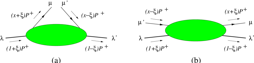
Figure 1: Representation of a generalized parton distribution in the region $\xi<x<1$. The flow of plus-momentum is indicated by arrows, and the labels $\lambda$, $\lambda^{\prime}$, $\mu$, $\mu^{\prime}$ denote helicities. (a) shows the ordering of lines as “proton in, quark out, quark back in, proton out” that is common for parton distributions. (b) displays the order “proton in, quark in, quark out, proton out” appropriate for a scattering amplitude.

In order to assign helicities to the quarks it is convenient to have them on-shell. A way to achieve this is to quantize the theory on the light-cone and to work in a noncovariant, Hamiltonian framework [12, 14]. In this framework, the dynamically independent (so called “good”) part of the fermion field is given by $\phi(z)=P_{+}\psi(z)$ with the projector $P_{+}=\frac{1}{2}\gamma^{-}\gamma^{+}$. It can be written as

$$\phi(z)=\frac{1}{\sqrt{2}}\left(\begin{array}[]{r}\phi_{R}(z)\\ \phi_{L}(z)\\ \phi_{R}(z)\\ -\phi_{L}(z)\end{array}\right),$$ (26)

where again we use the Dirac representation of four-spinors. At light-cone time $z^{+}=0$, the Fourier components of $\phi_{R}(z)$ are the annihilation operator for an on-shell quark with helicity $+\frac{1}{2}$ and the creation operator for an on-shell antiquark with helicity $-\frac{1}{2}$. Conversely, the Fourier components of $\phi_{L}(z)$ are the annihilation operator for an on-shell quark with helicity $-\frac{1}{2}$ and the creation operator for an on-shell antiquark with helicity $+\frac{1}{2}$. The operators occurring in the definitions of the quark distributions can be written as

$${\cal O}_{+,+}=\frac{1}{\sqrt{2}}\,\phi^{\dagger}_{R}\,\phi^{\phantom{\dagger}}_{R} = \frac{1}{4}\,\bar{\psi}\,\gamma^{+}(1+\gamma_{5})\,\psi,$$

$${\cal O}_{-,-}=\frac{1}{\sqrt{2}}\,\phi^{\dagger}_{L}\,\phi^{\phantom{\dagger}}_{L} = \frac{1}{4}\,\bar{\psi}\,\gamma^{+}(1-\gamma_{5})\,\psi,$$

$${\cal O}_{-,+}=\frac{1}{\sqrt{2}}\,\phi^{\dagger}_{L}\,\phi^{\phantom{\dagger}}_{R} = -\frac{i}{4}\,\bar{\psi}\,\sigma^{+1}(1+\gamma_{5})\,\psi=-\frac{i}{4}\,\bar{\psi}\,(\sigma^{+1}-i\sigma^{+2})\,\psi,$$

$${\cal O}_{+,-}=\frac{1}{\sqrt{2}}\,\phi^{\dagger}_{R}\,\phi^{\phantom{\dagger}}_{L} = \frac{i}{4}\,\bar{\psi}\,\sigma^{+1}(1-\gamma_{5})\,\psi\phantom{-}=\frac{i}{4}\,\bar{\psi}\,(\sigma^{+1}+i\sigma^{+2})\,\psi,\hskip 20.00003pt$$ (27)

where for brevity we have omitted the position arguments $\pm z/2$ of the field operators. For definiteness we will in the following restrict ourselves to the region $\xi<x<1$ of plus-momentum fractions, where the generalized quark distributions describe the emission of a quark with plus-momentum $(x+\xi)\,P^{+}$ and its reabsorption with plus-momentum $(x-\xi)\,P^{+}$.

We now are in a position to define the matrix elements

$$A_{\lambda^{\prime}\mu^{\prime},\lambda\mu} = \int\frac{dz^{-}}{2\pi}\,e^{ixP^{+}z^{-}}\langle p^{\prime},\lambda^{\prime}|\,{\cal O}_{\mu^{\prime},\mu}(z)\,|p,\lambda\rangle\Big{|}_{z^{+}=0,\,\mathbf{z}_{T}=0}$$

$$= \int\frac{d^{2}k_{T}}{(2\pi)^{3}}\left[\,\int dz^{-}\,d^{2}z_{T}\,e^{ik\cdot z}\,\langle p^{\prime},\lambda^{\prime}|\,{\cal O}_{\mu^{\prime},\mu}(z)\,|p,\lambda\rangle\,\right]_{z^{+}=0,\,k^{+}=xP^{+}}$$

for definite parton helicities $\mu$ and $\mu^{\prime}$. We remark that our labeling of the helicities corresponds to the ordering of lines shown in Fig. 1(a) and is different from the usual one for helicity amplitudes, represented in Fig. 1(b). Notice in Eq. (3) that in the noncovariant framework there is no longer an integration over the minus-momentum of the partons as there was in Eq. (25). One now keeps the condition $z^{+}=0$ in the bilocal operator since it is at that point where the field operators can be replaced in a simple manner by the creation and annihilation operators for on-shell partons. Put in a different way, the $k^{-}$ of the partons is not integrated over because it is fixed by the on-shell condition. We emphasize, however, that still one does integrate over the transverse parton momentum.

As we have discussed, the $A_{\lambda^{\prime}\mu^{\prime},\lambda\mu}$ are not exactly helicity amplitudes. What is important in our context is that they share several symmetry properties which are satisfied by helicity amplitudes. In particular, one has the relations

$$A_{-\lambda^{\prime}-\mu^{\prime},-\lambda-\mu}=(-1)^{\lambda^{\prime}-\mu^{\prime}-\lambda+\mu}\,A_{\lambda^{\prime}\mu^{\prime},\lambda\mu}$$ (29)

from parity invariance, provided one works in a reference frame where the momenta ${\mathbf{p}}$ and ${\mathbf{p}}^{\prime}$ lie in the $x$-$z$ plane, which we will do from now on. Explicit calculation gives

$$A_{++,++} = \sqrt{1-\xi^{2}}\left(\frac{H^{q}+\tilde{H}^{q}}{2}-\frac{\xi^{2}}{1-\xi^{2}}\,\frac{E^{q}+\tilde{E}^{q}}{2}\right),$$

$$A_{-+,-+} = \sqrt{1-\xi^{2}}\left(\frac{H^{q}-\tilde{H}^{q}}{2}-\frac{\xi^{2}}{1-\xi^{2}}\,\frac{E^{q}-\tilde{E}^{q}}{2}\right),$$

$$A_{++,-+} = -\epsilon\,\frac{\sqrt{t_{0}-t}}{2m}\,\frac{E^{q}-\xi\tilde{E}^{q}}{2},$$

$$A_{-+,++} = \epsilon\,\frac{\sqrt{t_{0}-t}}{2m}\,\frac{E^{q}+\xi\tilde{E}^{q}}{2},$$ (30)

in the quark helicity conserving sector, and

$$A_{++,+-} = \epsilon\,\frac{\sqrt{t_{0}-t}}{2m}\left(\tilde{H}_{T}^{q}+(1-\xi)\,\frac{E_{T}^{q}+\tilde{E}_{T}^{q}}{2}\right),$$

$$A_{-+,--} = \epsilon\,\frac{\sqrt{t_{0}-t}}{2m}\left(\tilde{H}_{T}^{q}+(1+\xi)\,\frac{E_{T}^{q}-\tilde{E}_{T}^{q}}{2}\right),$$

$$A_{++,--} = \sqrt{1-\xi^{2}}\left(H_{T}^{q}+\ \frac{t_{0}-t}{4m^{2}}\,\tilde{H}_{T}^{q}-\frac{\xi^{2}}{1-\xi^{2}}\,E_{T}^{q}+\frac{\xi}{1-\xi^{2}}\,\tilde{E}_{T}^{q}\right),$$

$$A_{-+,+-} = -\sqrt{1-\xi^{2}}\;\frac{t_{0}-t}{4m^{2}}\,\tilde{H}_{T}^{q}$$ (31)

for quark helicity flip, with the other helicity combinations given by parity invariance. Here

$$-t_{0}=\frac{4m^{2}\xi^{2}}{1-\xi^{2}}$$ (32)

is the minimum value of $-t$ for given $\xi$, and $\epsilon=\mathrm{sgn}(D^{1})$, where $D^{1}$ is the $x$-component of $D^{\alpha}=P^{+}\Delta^{\alpha}-\Delta^{+}P^{\alpha}$. The case $D^{1}=0$ corresponds to $t=t_{0}$ so that no ambiguity appears in Eqs. (3) and (3) at that point. Apart from restriction that ${\mathbf{p}}$ and ${\mathbf{p}}^{\prime}$ lie in $x$-$z$ plane, Eqs. (3) and (3) are valid for any choice of proton momenta.

We note in Eqs. (3) and (3) that the matrix elements where helicity is not conserved vanish like

$$\left(\frac{\sqrt{t_{0}-t}}{2m}\right)^{|\lambda^{\prime}-\mu^{\prime}-\lambda+\mu|}$$ (33)

in the collinear limit $t=t_{0}$, reflecting the fact that the mismatch of the helicities has to be compensated by one or two units of orbital angular momentum in order to ensure angular momentum conservation. One finds that in the collinear limit the distribution $\tilde{H}_{T}^{q}$ decouples, whereas in the forward limit, $t=0,\xi=0$, the only nonzero contribution comes from $H_{T}^{q}$, which in that limit reduces to the conventional quark transversity distribution, $H_{T}^{q}(x,0,0)=\delta q(x)$.

From Eq. (3) we explicitly see that the Dirac bilinears multiplying the distributions $H_{T}^{q}$, $\tilde{H}_{T}^{q}$, $E_{T}^{q}$, $\tilde{E}_{T}^{q}$ in the decomposition (3) are linearly independent. If the right-hand side of (3) is to be identically zero, then all four helicity combinations in Eq. (3) must vanish, and this is only the case if all four distributions are zero.

Let us now see why the counting argument of Hoodbhoy and Ji [9] does not apply. They invoke that with the constraints from parity and time reversal invariance there are only six independent helicity amplitudes for elastic quark-proton scattering. This is correct, but closer inspection reveals that three of these amplitudes flip the helicity of the quark and three do not. This does not correspond to the four non-flip distributions in Eq. (2) and the two flip distributions $H_{T}^{q}$ and $E_{T}^{q}$ considered in Ref. [9].

At this point we must remember that the matrix elements defining generalized parton distributions are not helicity amplitudes in the strict sense. Time reversal exchanges initial and final state momenta. For usual helicity amplitudes, this exchange can be compensated for by a suitable rotation in the center-of-mass of the collision, where the three-momenta of the incoming and outgoing particles have equal length. The matrix elements (2) and (3), however, refer to a fixed light-cone axis with respect to which transverse, plus- and minus-momenta are defined. Notably, the integration over transverse parton momenta in Eq. (3) refers to this particular axis. Time reversal changes $\xi$ into $-\xi$ and thus provides the relations (6) and (7). One might perform a Lorentz transformation to another frame in order to compensate for this change, but such a transformation will not leave the light-cone axis invariant. In the new frame, the generalized parton distributions are then no longer given as in Eq. (3), i.e., by an integration over the transverse parton momentum with all plus-momenta fixed.

One may ask whether it is possible to find further time reversal constraints, for instance by first considering the matrix elements that correspond to (3) but are not integrated over the parton $\mathbf{k}_{T}$, trying to obtain constraints of the type one has for usual helicity amplitudes, and then performing the integrations over $\mathbf{k}_{T}$. We will not pursue this here, but remark that even for fixed $k^{+}$ and $\mathbf{k}_{T}$ one still has singled out a light-cone direction, namely by the condition $z^{+}=0$ in the matrix element (3).

The argument just given indicates however that the number of independent structures is reduced from eight to six in the case $\xi=0$ (note that this does not imply $p=p^{\prime}$ since one can still have $t\neq 0$). Clearly, the change $\xi\to-\xi$ of time reversal is of no consequence then. Indeed, $\tilde{E}_{T}^{q}$ vanishes at $\xi=0$ due to the constraint (7). At the same point $\tilde{E}^{q}$, although nonzero, decouples from all amplitudes because in its definition (2) it is multiplied with $\Delta^{+}=-2\xi P^{+}$. Inspecting Eqs. (3) and (3) we then find $A_{++,-+}=-A_{-+,++}$ and $A_{++,+-}=-A_{+-,++}$, where in the second equation we have used the parity relation (29). These are precisely the constraints on usual helicity amplitudes arising from time reversal invariance. We see that one of the two distributions that have thus been removed flips quark helicity, while the other does not, in accordance with our remark above.

The main results of our discussion can be generalized to targets with arbitrary spin. As is well known, the number of ordinary quark or gluon distributions is equal to the corresponding number of independent helicity amplitudes allowed by parity and time reversal invariance (and by helicity conservation, since one is dealing with forward amplitudes) [5]. For generalized parton distributions, the counting works differently. Their number is obtained from counting the helicity amplitudes under the constraints of parity invariance only. Time reversal invariance determines the behavior of the generalized distributions under exchange of the hadron momenta ($\xi\to-\xi$) and fixes their phase.

4 Gluon helicity flip distributions

We now turn to gluon distributions. As is well known, there are again four distributions conserving gluon helicity,

$$\frac{1}{P^{+}}\int\frac{dz^{-}}{2\pi}\,e^{ixP^{+}z^{-}}\langle p^{\prime},\lambda^{\prime}|\,F^{+i}(-{\textstyle\frac{1}{2}}z)\,F^{+i}({\textstyle\frac{1}{2}}z)\,\,|p,\lambda\rangle\Big{|}_{z^{+}=0,\,\mathbf{z}_{T}=0}$$

$$= \frac{1}{2P^{+}}\bar{u}(p^{\prime},\lambda^{\prime})\left[H^{g}\,\gamma^{+}+E^{g}\,\frac{i\sigma^{+\alpha}\Delta_{\alpha}}{2m}\right]u(p,\lambda),$$

$$-\frac{i}{P^{+}}\int\frac{dz^{-}}{2\pi}\,e^{ixP^{+}z^{-}}\langle p^{\prime},\lambda^{\prime}|\,F^{+i}(-{\textstyle\frac{1}{2}}z)\,\tilde{F}^{+i}({\textstyle\frac{1}{2}}z)\,\,|p,\lambda\rangle\Big{|}_{z^{+}=0,\,\mathbf{z}_{T}=0}$$ (34)

$$= \frac{1}{2P^{+}}\bar{u}(p^{\prime},\lambda^{\prime})\left[\tilde{H}^{g}\,\gamma^{+}\gamma_{5}+\tilde{E}^{g}\,\frac{\gamma_{5}\Delta^{+}}{2m}\,\,\right]u(p,\lambda),$$

where $\tilde{F}^{\alpha\beta}=\frac{1}{2}\epsilon^{\alpha\beta\gamma\delta}F_{\gamma\delta}$ is the dual field strength tensor and a summation over $i=1,2$ is implied. These definitions differ from those of Hoodbhoy and Ji [9], ours are normalized such that in the forward limit one has

$$H^{g}(x,0,0)=xg(x),\hskip 20.00003pt\tilde{H}^{g}(x,0,0)=x\Delta g(x)$$ (35)

with the usual spin averaged and spin dependent gluon densities $g(x)$ and $\Delta g(x)$. Compared with Ref. [9], we have

$$2xH_{g}\Big{|}_{\mathrm{Ref.~{}[9]}}=H^{g}\Big{|}_{\mathrm{here}},$$ (36)

and analogous relations for $E^{g}$, $\tilde{H}^{g}$, and $\tilde{E}^{g}$. The gluon helicity flip distributions involve the gluon tensor operator ${\mathbf{S}}F^{+i}(-{\textstyle\frac{1}{2}}z)\,F^{+j}({\textstyle\frac{1}{2}}z)$, where ${\mathbf{S}}$ denotes symmetrization in $i$ and $j$ and subtraction of the trace. To parameterize this structure we use the same Dirac bilinears as in the definition (3) for quarks and introduce

$$-\frac{1}{P^{+}}\int\frac{dz^{-}}{2\pi}\,e^{ixP^{+}z^{-}}\langle p^{\prime},\lambda^{\prime}|\,{\mathbf{S}}F^{+i}(-{\textstyle\frac{1}{2}}z)\,F^{+j}({\textstyle\frac{1}{2}}z)\,|p,\lambda\rangle\Big{|}_{z^{+}=0,\,\mathbf{z}_{T}=0}$$ (37)

$$= {\mathbf{S}}\,\frac{1}{2P^{+}}\,\frac{P^{+}\Delta^{j}-\Delta^{+}P^{j}}{2mP^{+}}$$

$$\times \bar{u}(p^{\prime},\lambda^{\prime})\left[H_{T}^{g}\,i\sigma^{+i}+\tilde{H}_{T}^{g}\,\frac{P^{+}\Delta^{i}-\Delta^{+}P^{i}}{m^{2}}\right.$$

$$\left.\hskip 28.00006pt{}+E_{T}^{g}\,\frac{\gamma^{+}\Delta^{i}-\Delta^{+}\gamma^{i}}{2m}+\tilde{E}_{T}^{g}\,\frac{\gamma^{+}P^{i}-P^{+}\gamma^{i}}{m}\,\right]u(p,\lambda).\hskip 20.00003pt$$

Our distributions $H_{T}^{g}$ and $E_{T}^{g}$ are identical with $H_{G}^{T}$ and $E_{G}^{T}$ used in [10], and related with those of Hoodbhoy and Ji by

$$-2xH_{Tg}\Big{|}_{\mathrm{Ref.~{}[9]}}=H_{T}^{g}\Big{|}_{\mathrm{here}},\hskip 20.00003pt-2xE_{Tg}\Big{|}_{\mathrm{Ref.~{}[9]}}=E_{T}^{g}\Big{|}_{\mathrm{here}}.$$ (38)

As in the case of quarks, one can see that there are at most four independent distributions to parameterize the matrix element (37) with the constraints of parity invariance, and we have shown in Section 3 that the four Dirac bilinears are linearly independent.

The support of all eight gluon distributions is $-1\leq x\leq 1$. It is easy to see that $\tilde{H}^{g}(x,\xi,t)$ and $\tilde{E}^{g}(x,\xi,t)$ are odd in $x$, whereas the other six distributions are even. Time reversal invariance leads to the same constraints as in the case of quarks, and Eqs. (6) to (9) remain valid with the subscripts $q$ changed into $g$. In particular, one also finds that the first moment in $x$ of $\tilde{E}_{T}^{g}$ has to vanish, in analogy to Eq. (11).

To find a helicity representation for the gluon distributions we use again the framework of light-cone quantization. We recall that in the gauge $A^{+}=0$ we are working in one has $F^{+i}=\partial^{+}A^{i}$. The transverse components of the gluon potential $A^{i}$ are the “good” components of the field, and combinations with definite helicity are projected out by contracting them with the two-dimensional polarization vectors

$$\epsilon(+)=-\frac{1}{\sqrt{2}}\left(\begin{array}[]{c}1\\ i\end{array}\right),\hskip 30.00005pt\epsilon(-)=\frac{1}{\sqrt{2}}\left(\begin{array}[]{c}1\\ -i\end{array}\right).$$ (39)

In the region $\xi<x<1$, where the operator $F^{+i}(-\frac{1}{2}z)$ is associated with an incoming and $F^{+j}(\frac{1}{2}z)$ with an outgoing gluon, we then define helicity combinations

$$A_{\lambda^{\prime}\mu^{\prime},\lambda\mu} = \frac{1}{P^{+}}\int\frac{dz^{-}}{2\pi}\,e^{ixP^{+}z^{-}}$$ (40)

$$\times \langle p^{\prime},s^{\prime}|\,\epsilon^{i}(\mu^{\prime})F^{+i}(-{\textstyle\frac{1}{2}}z)\,F^{+j}({\textstyle\frac{1}{2}}z)\epsilon^{*j}(\mu)\,|p,s\rangle\Big{|}_{z^{+}=0,\,\mathbf{z}_{T}=0}\,,\hskip 20.00003pt$$

where summation over $i,j=1,2$ is understood. One easily sees that the matrix elements $A_{\lambda^{\prime}\mu^{\prime},\lambda\mu}$ which conserve gluon helicity read exactly as those in Eq. (3) with the superscript $q$ changed to $g$ in the distributions $H$, $\tilde{H}$, $E$, $\tilde{E}$. For gluon helicity flip we find

$$A_{++,+-} = \sqrt{1-\xi^{2}}\;\frac{t_{0}-t}{4m^{2}}\left(\tilde{H}_{T}^{g}+(1-\xi)\,\frac{E_{T}^{g}+\tilde{E}_{T}^{g}}{2}\right),$$

$$A_{-+,--} = \sqrt{1-\xi^{2}}\;\frac{t_{0}-t}{4m^{2}}\left(\tilde{H}_{T}^{g}+(1+\xi)\,\frac{E_{T}^{g}-\tilde{E}_{T}^{g}}{2}\right),$$

$$A_{++,--} = \epsilon\,(1-\xi^{2})\,\frac{\sqrt{t_{0}-t}}{2m}$$

$$\times\left(H_{T}^{g}+\ \frac{t_{0}-t}{4m^{2}}\,\tilde{H}_{T}^{g}-\frac{\xi^{2}}{1-\xi^{2}}\,E_{T}^{g}+\frac{\xi}{1-\xi^{2}}\,\tilde{E}_{T}^{g}\right),$$

$$A_{-+,+-} = -\epsilon\,(1-\xi^{2})\,\frac{\sqrt{t_{0}-t}^{\,3}}{8m^{3}}\,\tilde{H}_{T}^{g}\,.$$ (41)

The remaining helicity combinations are given by the parity relation (29). Notice that all gluon helicity flip matrix elements go to zero with a factor (33) in the collinear limit, $t=t_{0}$, where angular momentum conservation requires $\lambda-\mu=\lambda^{\prime}-\mu^{\prime}$. In other words, the gluon helicity flip distributions for a spin $\frac{1}{2}$ target decouple from any observable for collinear scattering.

5 Compton scattering

The generalized gluon helicity flip distributions appear in deeply virtual Compton scattering, i.e., in the process $\gamma^{*}p\to\gamma p$ at large photon virtuality $Q^{2}$, large c.m. energy, and small squared momentum transfer $t$. This process is observable in electroproduction, $ep\to e\gamma p$.

It is easy to see that to leading order in $1/Q$, the gluon helicity flip distributions only contribute to the $\gamma^{*}p\to\gamma p$ amplitudes where the photon helicity is flipped by two units [8]. This is because, to that accuracy, the hard scattering subprocess is collinear, so that the gluon helicity flip needs to be compensated by the photons. Conversely, to leading order in $1/Q$, it is only the helicity flip gluon distributions that appear in the photon helicity flip amplitudes. Although only coming in at order $\alpha_{s}$, these distributions thus provide the leading contribution to photon helicity flip. This is different for the helicity conserving gluon distributions (4). They contribute at order $\alpha_{s}$ to the photon helicity conserving amplitudes, which receive Born level contributions from the quark distributions (2). Given that the different photon helicity amplitudes can be separated by the measurement of angular distributions in the final state [8], one may thus be able to experimentally access the gluon helicity flip distributions in a rather direct and clean way.

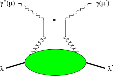
Figure 2: A Feynman diagram for the photon helicity flip amplitude in deeply virtual Compton scattering. The remaining diagrams are obtained by appropriate permutations of the photon and gluon lines. Greek letters label helicities, and the relevant combinations are $(\mu^{\prime},\mu)=(1,-1)$ and $(\mu^{\prime},\mu)=(-1,1)$.

The Feynman diagrams involving gluon helicity flip (see Fig. 2) have been calculated by two groups [9, 10]. They give the relevant $\gamma^{*}p\to\gamma p$ amplitudes to leading order in $1/Q$ as

$$e^{2}M_{\lambda^{\prime}\mu^{\prime},\lambda\mu} = -\frac{\alpha_{s}}{2\pi}\sum_{q}e^{2}e_{q}^{2}\,\int_{-1}^{1}dx\,\frac{A_{\lambda^{\prime}\mu^{\prime},\lambda\mu}(x,\xi,t)}{(\xi-x-i\epsilon)(\xi+x-i\epsilon)}$$ (42)

for $(\mu^{\prime},\mu)=(1,-1)$ and $(\mu^{\prime},\mu)=(-1,1)$, where $\mu^{\prime}$ and $\mu$ in $M_{\lambda^{\prime}\mu^{\prime},\lambda\mu}$ denote the respective helicities of the outgoing and incoming photon. The matrix elements $A_{\lambda^{\prime}\mu^{\prime},\lambda\mu}$ are given by Eqs. (4) and (29). Our polarization vectors for both photon states read $\epsilon(\pm)=(0,\mp 1,i,0)/\sqrt{2}$, up to corrections in $1/Q$, where it is understood that in our reference frame the photons are left-moving and the protons right-moving.

Whether the gluon helicity flip distributions can be accessed experimentally at a given value of $Q^{2}$, depends on their size. They have to be large enough to compensate for the factor $\alpha_{s}/\pi$ in the leading-twist contribution (42), which competes with power suppressed terms that already start at zeroth order in $\alpha_{s}$. Unfortunately, nothing is presently known about the size of gluon helicity flip distributions in the proton.

In which combinations the distributions $H_{T}^{g}$, $\tilde{H}_{T}^{g}$, $E_{T}^{g}$, $\tilde{E}_{T}^{g}$ appear in the cross section of $ep\to e\gamma p$, shall not be studied here in detail. As an example we mention only their contribution to the interference term between the Compton and the Bethe-Heitler processes, where they give rise to a $\cos 3\varphi$ angular distribution (for more details we refer to [8]). With unpolarized electrons and protons, they appear in the combination

$$\frac{\sqrt{t_{0}-t}^{\,3}}{8m^{3}}\left[H_{T}^{g}\,F_{2}^{\phantom{g}}-E_{T}^{g}\,F_{1}^{\phantom{g}}-2\tilde{H}_{T}^{g}\left(F_{1}^{\phantom{g}}+\frac{t}{4m^{2}}\,F_{2}^{\phantom{g}}\right)\right]\cos 3\varphi,$$ (43)

where $F_{1}$ and $F_{2}$ are the Dirac and Pauli form factor of the proton, respectively. It is amusing to note that the distribution $\tilde{E}_{T}^{g}$ does not appear in this term, just as the parton helicity conserving distributions $\tilde{E}^{q}$ and $\tilde{E}^{g}$ are absent in the corresponding $\cos\varphi$ term, see Eq. (30) of [17]. $\tilde{E}_{T}^{g}$ is however present in the contribution to the cross section from the Compton process alone, and also in the interference term with the Bethe-Heitler process if the initial proton is polarized.

6 Summary

We have given a complete set of generalized parton helicity flip distributions for a spin $\frac{1}{2}$ target. Both in the quark and gluon sector there are four independent distributions, i.e., two more than previously considered in the literature [9, 10].

The constraints of parity invariance are very similar for ordinary and generalized parton distributions and for the helicity amplitudes of two-particle elastic scattering, as is embodied in Eq. (29). This is not the case for invariance under time reversal, which acts to reduce the number of independent helicity amplitudes and of ordinary parton distributions, but not of generalized ones. This can be traced back to the dependence of generalized parton distributions on the momentum fraction $\xi$ or, more broadly speaking, to the fact that generalized distributions not only depend on two independent hadron momenta, but also on a light-cone direction. Time reversal symmetry determines the behavior of generalized distribution under $\xi\to-\xi$ and fixes their phase. For counting the independent generalized distributions of targets with arbitrary spin, one can still use the analogy with helicity amplitudes, but must at that stage only use the constraints from parity invariance, not those from time reversal.

As a by-product of our investigation we found that time reversal invariance reduces the number of form factors of the local quark tensor current $\bar{\psi}\,\sigma^{\alpha\beta}\,\psi$ from four to three. This illustrates that this symmetry also acts in slightly different, although related ways on generalized parton distributions and on elastic form factors.

At present we do not know a physical process that would give access to generalized quark helicity distributions. Their gluonic counterparts can be rather cleanly investigated in deeply virtual Compton scattering, under the condition that they are large enough. This would be extremely interesting because, as that they do not mix with the quark sector under evolution, gluon helicity flip distributions should provide a rather unique glimpse into the dynamics of glue in the nucleon.

Appendix

In this appendix we study the form factor decomposition of the tensor current (10) for the proton, which is also needed for the parameterization of quark helicity flip distributions. We will classify the Dirac bilinears

$$\bar{u}(p^{\prime},\lambda^{\prime})\,\Gamma_{n}^{\alpha\beta}\,u(p,\lambda)$$ (44)

where $\Gamma_{n}^{\alpha\beta}$ is a matrix in Dirac space and antisymmetric in the Lorentz indices $\alpha$ and $\beta$. By parity invariance $\Gamma_{n}^{\alpha\beta}$ must be a Lorentz tensor, not a pseudotensor. We do not use any restrictions from time reversal at this point. Let us show that an independent set of bilinears can be chosen as the one on the right-hand side of Eq. (3). For this, we use the equations of motion for spinors, i.e., the Gordon identities

$$2m\,\bar{u}(p^{\prime})\,\gamma^{\alpha}\,u(p) = \bar{u}(p^{\prime})\,\left[(p^{\prime}+p)^{\alpha}+i\sigma^{\alpha\beta}(p^{\prime}-p)_{\beta}\right]u(p),$$ (45)

$$2m\,\bar{u}(p^{\prime})\,\gamma^{\alpha}\gamma_{5}\,u(p) = \bar{u}(p^{\prime})\,\left[\gamma_{5}(p^{\prime}-p)^{\alpha}+i\sigma^{\alpha\beta}\gamma_{5}(p^{\prime}+p)_{\beta}\right]u(p),\hskip 20.00003pt$$ (46)

and furthermore

$$0 = \bar{u}(p^{\prime})\,\left[(p^{\prime}-p)^{\alpha}+i\sigma^{\alpha\beta}(p^{\prime}+p)_{\beta}\right]u(p),$$ (47)

$$0 = \bar{u}(p^{\prime})\,\left[\gamma_{5}(p^{\prime}+p)^{\alpha}+i\sigma^{\alpha\beta}\gamma_{5}(p^{\prime}-p)_{\beta}\right]u(p).$$ (48)

Now we show that all possible parity even structures in Eq. (44) can be reduced to

$$\Gamma_{1}^{\alpha\beta}=i\sigma^{\alpha\beta},\hskip 41.00012pt \Gamma_{2}^{\alpha\beta}=P^{\alpha}\Delta^{\beta}-\Delta^{\alpha}P^{\beta},$$

$$\Gamma_{3}^{\alpha\beta}=\gamma^{\alpha}\Delta^{\beta}-\Delta^{\alpha}\gamma^{\beta}, \Gamma_{4}^{\alpha\beta}=\gamma^{\alpha}P^{\beta}-P^{\alpha}\gamma^{\beta}.$$ (49)

The $\Gamma_{n}^{\alpha\beta}$ must be constructed out of invariants and the vectors $P$ and $\Delta$. We treat all possible Dirac currents in turn:

1. axial vector current ($\bar{u}\,\gamma^{\delta}\gamma_{5}\,u$): We can use the Gordon identity (46) and replace it by the pseudoscalar current and by $\bar{u}\,i\sigma^{\gamma\delta}\gamma_{5}\,u$. Then go to 2 and 3.

2. pseudoscalar current ($\bar{u}\,\gamma_{5}\,u$): Due to parity invariance, this must be multiplied with a pseudotensor of rank 2. The only possible choice is $\epsilon^{\alpha\beta\gamma\delta}\,\Delta_{\gamma}P_{\delta}$. Using Eq. (48), we can eliminate $\bar{u}\,\gamma_{5}P_{\delta}\,u$ in favor of $\bar{u}\,i\sigma^{\gamma\delta}\gamma_{5}\,u$. Then go to 3.

3. pseudotensor current ($\bar{u}\,i\sigma^{\gamma\delta}\gamma_{5}\,u$): can be replaced by the tensor current using Eq. (4). Then go to 4.

4. tensor current ($\bar{u}\,i\sigma^{\gamma\delta}\,u$): If any of the indices $\gamma$ or $\delta$ is contracted with $P$ or $\Delta$, we can express this current in terms of the scalar and vector current using the identities (45) and (47). The contraction of $\gamma$ and $\delta$ with the $\epsilon$-tensor is not allowed by parity invariance, so that the only possibility left gives $\Gamma_{1}^{\alpha\beta}=i\sigma^{\alpha\beta}$.

5. vector current ($\bar{u}\,\gamma^{\delta}\,u$): If the index $\delta$ is contracted with $P$ or $\Delta$ we can use the equations of motion to obtain the scalar current or zero. Again we cannot contract with the $\epsilon$-tensor because of parity invariance. The only possibilities left to form an antisymmetric tensor of rank 2 are thus those in $\Gamma_{3}$ and $\Gamma_{4}$.

6. scalar current ($\bar{u}u$): must be multiplied with an antisymmetric tensor of rank 2. We cannot use the $\epsilon$-tensor because of parity constraints, so the only possibility left leads to $\Gamma_{2}$.

As we discussed in Section 2, time reversal invariance forbids $\Gamma_{4}$ in the decomposition of the local current matrix element $T^{\alpha\beta}$ in (10), but not in the case of the bilocal current (3) defining the quark helicity flip distributions. The second moment $\int dx\,x\tilde{E}_{T}^{q}(x,\xi,t)$ is connected with the local matrix element

$$\langle p^{\prime},\lambda^{\prime}|\,\bar{\psi}(0)\,\raisebox{0.86108pt}{$\stackrel{{\scriptstyle\leftrightarrow}}{{\partial}}{}^{\!\!+}$}i\sigma^{+i}\,\psi(0)\,\,|p,\lambda\rangle.$$ (50)

Now we do have four linearly independent tensors respecting the constraints of both parity and time reversal invariance, namely $P_{\phantom{1}}^{+}\Gamma_{1}^{+i}$, $P_{\phantom{1}}^{+}\Gamma_{2}^{+i}$ , $P_{\phantom{1}}^{+}\Gamma_{3}^{+i}$, and $\Delta_{\phantom{1}}^{+}\Gamma_{4}^{i+}$.

References

• [1] D. Müller, D. Robaschik, B. Geyer, F. M. Dittes and J. Hořejši, Fortsch. Phys.  42 (1994) 101 [hep-ph/9812448].
• [2] X. Ji, Phys. Rev. Lett.  78 (1997) 610 [hep-ph/9603249];
A. V. Radyushkin, Phys. Rev.  D56 (1997) 5524 [hep-ph/9704207].
• [3] P. R. Saull (ZEUS Collaboration), hep-ex/0003030;
L. Favart (H1 Collaboration), hep-ex/0101046;
M. Amarian (HERMES Collaboration), talk given at the 14th International Spin Physics Symposium (SPIN 2000), Osaka, Japan, Oct. 2000, to appear in the Proceedings.
• [4] J. P. Ralston and D. E. Soper, Nucl. Phys.  B152 (1979) 109.
• [5] R. L. Jaffe, hep-ph/9602236.
• [6] J. C. Collins, L. Frankfurt and M. Strikman, Phys. Rev. D 56 (1997) 2982 [hep-ph/9611433].
• [7] L. Mankiewicz, G. Piller and T. Weigl, Eur. Phys. J.  C5 (1998) 119 [hep-ph/9711227];
M. Diehl, T. Gousset and B. Pire, Phys. Rev.  D59 (1999) 034023 [hep-ph/9808479];
J. C. Collins and M. Diehl, Phys. Rev.  D61 (2000) 114015 [hep-ph/9907498].
• [8] M. Diehl, T. Gousset, B. Pire and J. P. Ralston, Phys. Lett.  B411 (1997) 193 [hep-ph/9706344].
• [9] P. Hoodbhoy and X. Ji, Phys. Rev.  D58 (1998) 054006 [hep-ph/9801369].
• [10] A. V. Belitsky and D. Müller, Phys. Lett.  B486 (2000) 369 [hep-ph/0005028].
• [11] R. L. Jaffe and A. Manohar, Phys. Lett.  B223 (1989) 218;
X. Artru and M. Mekhfi, Z. Phys.  C45 (1990) 669.
• [12] J. B. Kogut and D. E. Soper, Phys. Rev.  D1 (1970) 2901.
• [13] M. Diehl, T. Feldmann, R. Jakob and P. Kroll, hep-ph/0009255.
• [14] S. J. Brodsky, H. Pauli and S. S. Pinsky, Phys. Rept. 301 (1998) 299 [hep-ph/9705477].
• [15] P. V. Landshoff, J. C. Polkinghorne and R. D. Short, Nucl. Phys.  B28 (1971) 225.
• [16] R. L. Jaffe, Nucl. Phys.  B229 (1983) 205;
M. Diehl and T. Gousset, Phys. Lett.  B428 (1998) 359 [hep-ph/9801233].
• [17] A. V. Belitsky, D. Müller, L. Niedermeier and A. Schäfer, Nucl. Phys. B593 (2001) 289 [hep-ph/0004059].