Abstract

We consider the possibility that after operations at the LHC and $e^{+}e^{-}$ Linear Colliders a Higgs boson will be discovered, but no signal of New Physics will be found (Standard-Model-like scenario). This can occur in the Standard Model (SM) as well as in other models, including the Two-Higgs-Doublet Model (2HDM), the MSSM, etc. Experiments at a Photon Collider can resolve these cases.

In this paper we compare the SM and the 2HDM (II). In the analysis we use as independent quantities the ratios, to the SM values, of couplings of the observed Higgs boson to gauge bosons, and to up and down-type quarks (basic couplings). We derive a relation between these ratios within the 2HDM (II), a pattern relation. With the aid of this relation, different possible realizations of an SM-like scenario are found. For these realizations, we calculate the loop couplings of the Higgs boson with $\gamma\gamma$ and $Z\gamma$, and also with gluons, taking into account the expected accuracy in the measurements of the basic couplings. The obtained deviation of the two-photon width from its SM value is generally higher than the expected inaccuracy in the measurement of $\Gamma_{\gamma\gamma}$ at a Photon Collider. The result is sensitive to the parameters of the Higgs self interaction.

1 Introduction

In a widely discussed optimistic scenario, new physics will reveal itself immediately above the Fermi scale $v=246$ GeV, and new particles will be sufficiently light that they can be discovered at the Tevatron and the LHC. Linear Colliders, including a Photon Collider mode ($\gamma\gamma$ and $e\gamma$ [1]), would be machines for measuring precise values of coupling constants and exploring in detail supersymmetry, etc. [2].

However, it could happen that the Higgs boson $h$ will be discovered, but no signal of New Physics will be found, beyond the Standard Model (SM). In this SM-like scenario, in particular, the Higgs boson partial widths or coupling constants squared are precisely measured, being in agreement with the SM within the experimental accuracies. This can happen not only in the SM, but also if Nature is described by some other theory, for example, the Two-Higgs-Doublet Model (2HDM) or the Minimal Supersymmetric Standard Model (MSSM). In this case the main task for new colliders will be to search for signals of new physics via deviations of observed quantities from SM predictions. After LHC and $e^{+}e^{-}$ Linear Collider operations the study of Higgs boson production at a Photon Collider offers excellent opportunities for this [3]. Indeed, in the SM and in its extensions, all fundamental charged particles contribute to the $h\gamma\gamma$ and $hZ\gamma$ effective couplings which can be tested at such a collider. Besides, these couplings are absent in the SM at tree level, appearing only at the loop level. Therefore, the background for signals of new physics will be relatively lower here than in processes which are allowed at tree level of the SM. We focus our consideration on the era after LHC and $e^{+}e^{-}$ Linear Collider operations, all numbers for experimental uncertainties are related to this period. However, we discuss additionally some effects for the preceding era (but after discovery of the Higgs boson).

In the 2HDM and MSSM the observed Higgs boson can be either one of two neutral CP-even scalars, $h$ or $H$ ($M_{h}<M_{H}$). In the present paper we compare the SM and the SM-like scenario in the 2HDM in its Model II variant of couplings with fermions, 2HDM (II). We derive a specific constraint for the couplings of these scalars to fermions and gauge bosons, valid in the 2HDM (II) and MSSM — the pattern relation. It helps us to obtain additional, as compared to anticipated future data, constraints for the couplings of the observed Higgs scalar to fermions and $W$ or $Z$ bosons.

To investigate how one can resolve the SM and the 2HDM (II) in the SM-like scenario, we calculate the $\gamma\gamma$ and $Z\gamma$ partial widths of the Higgs boson. We found that generally the $\gamma\gamma$ width deviates sufficiently from the corresponding SM values that one can distinguish models with the anticipated data, and measuring the $Z\gamma$ width can support this conclusion.

Besides, for some sets of coupling constants which are possible within the SM-like scenario, the models can be distinguished via a study of the two-photon and (or) two-gluon widths even before Photon Collider operations, at the Tevatron, the LHC or an $e^{+}e^{-}$ Linear Collider.

In a forthcoming paper we plan to study the MSSM in this same SM-like scenario, taking into account the anticipated improvement in the precision of the Higgs boson two-photon width.

2 Standard-Model-like scenario

We now consider the following scenario, referred to below as the SM-like scenario. It is given by the following criteria (whose precise formulations vary with time):

1. One Higgs boson will be discovered (with mass above today’s limit for an SM Higgs boson, 115 GeV [6]). It can be either the Higgs boson of the SM or one out of several neutral scalars of some other model, such as the 2HDM or the MSSM.

2. No other Higgs boson will be discovered. It means that other Higgs bosons, if they exist, are either weakly coupled with the $Z$ and $W$ bosons, gluons and quarks, or sufficiently heavy to escape (direct or indirect) observation, $M_{H},\;M_{A},\;M_{H^{\pm}}>{\cal O}(800\mbox{ GeV})$ [7].

3. All other new particles that may exist are heavier than the discovery limits of LHC and the $e^{+}e^{-}$ Linear Collider.

4. The measured decay widths of this Higgs boson (or coupling constants squared) to other particles, $\Gamma_{i}^{\rm exp}$, will be in agreement with their SM values $\Gamma_{i}^{\rm SM}$ within the experimental precision $\delta_{i}$

   $$\left|\frac{\Gamma_{i}^{\rm exp}}{\Gamma_{i}^{\rm SM}}-1\right|\mathrel{\hbox to0.0pt{\raise 2.5pt\hbox{$<$}\hss}\lower 2.5pt\hbox{$\sim$}}\delta_{i}\ll 1.$$ (1)

   The values $\delta_{i}$ will change with time. In our numerical studies we use the most precise estimates for the $e^{+}e^{-}$ Linear Collider, see Eq. (3). Note that even if all $\Gamma^{\rm exp}_{i}/\Gamma^{\rm SM}_{i}$=1 for $i=q,\ell,W$ or $Z$, the SM could still be violated (due to different signs of coupling constants and the existence of additional particles like a charged Higgs boson).

This scenario is realized, for example, for coupling constants corresponding to the decoupling limit for a particular version of the 2HDM (II) [4] or in the MSSM [4, 5]. The decoupling limit considered for the 2HDM (II) or in the MSSM is usually determined as that in which all coupling constants of the lightest Higgs boson are very close to the SM values irrespective of their experimental inaccuracies, assuming that the observed neutral Higgs boson is the lightest one. Besides, all other particles, Higgs particles and (in the MSSM) super-particles, are assumed to be very heavy. Further “natural” assumptions, which are valid in the MSSM but not necessarily in the 2HDM, are added in the treatment of the decoupling limit in Ref. [4]. Such a situation can be realized in our SM-like scenario. However, the SM-like scenario also permits other realizations which for the 2HDM (II) are discussed below.

3 Couplings in the SM-like scenario

3.1 Expected precision of measured SM Higgs couplings

Let $\delta_{i}$ be the relative experimental uncertainty in the partial width of a considered Higgs boson, $\Gamma_{i}^{\rm exp}$ (or coupling constants squared)

$$\delta_{i}=\frac{\delta\Gamma_{i}^{\rm exp}}{\Gamma_{i}^{\rm exp}}.$$ (2)

Actually, often combinations of partial widths are measured (like branching ratios) and experimental estimates are obtained for these quantities. Nevertheless, in our numerical study (which should be updated after actual experimentation), we use the values obtained for uncertainties of branching ratios etc., for the $\delta_{i}$ themselves.

At the LHC, the expected relative uncertainties (2) for the SM Higgs particle are of the order of 10–20% [7]. At the TESLA $e^{+}e^{-}$ collider the discussed production cross sections are expected to be measured with a significantly higher precision (at the same SM Higgs boson mass). At $M_{h}\leq 140$ GeV (where the $b\bar{b}$ decay channel is dominant) and with integrated luminosity 500–1000 fb^-1 one can expect [8, 9]:

$$\begin{array}[]{llll}\delta_{b}=0.024,&\delta_{\tau}=0.05,&\delta_{c}=0.083,&\delta_{t}=0.055,\\ \delta_{Z}=0.01,&\delta_{W}=0.054,&\delta_{g}=0.055,&\delta_{\gamma}=0.19.\end{array}$$ (3)

In contrast to other quantities here, the numbers for $\delta_{Z}$ and $\delta_{t}$ are for coupling constants from the analysis of the corresponding cross sections (not of branching ratios like the others). The first one will be obtained via the study of Higgs-strahlung by the recoil mass method, the second via comparison of the cross section $e^{+}e^{-}\to t\bar{t}h$ with that of Higgs-strahlung.

Experiments at Photon Colliders open new perspectives. In particular, even with an integrated luminosity of a $\gamma\gamma$ collider in the high energy peak of about $40$ fb^-1 (which is at least 5 times less than that discussed in recent proposals [11]), a $\gamma\gamma$ collider makes it possible to improve on the accuracy in measuring the $h\gamma\gamma$ width (via $b\bar{b}$ decay) up to [12]:

$$\delta_{\gamma}=0.02\quad\mbox{ for }M_{h}<140\mbox{ GeV}\,.$$ (4)

This improvement is crucial for the considered problem.

At $M_{h}>140$ GeV the other decay channels and production mechanisms become important and the above uncertainties change strongly. The dependencies of some of these uncertainties on the Higgs boson mass are presented in Ref. [8]. For the Higgs boson production at a Photon Collider one should study it via the $WW^{*}$ and $ZZ^{*}$ decay modes (instead of $b\bar{b}$) to find the accuracy in the measurement of $\Gamma_{h\gamma\gamma}$.

The accuracy in the measurement of the effective $hZ\gamma$ coupling (in the process $e\gamma\to eh$) is evidently not so high, it requires a separate study.

The value of the considered (SM-like) Higgs boson mass is expected to be obtained with very high accuracy, 40–90 MeV depending on the mass [8]. Therefore, we will not consider the uncertainty in the determination of the SM-width arising from the inaccuracy in the Higgs boson mass.

3.2 Limits on coupling constants from future data

In our discussion we use quantities whose deviations from unity for the observed Higgs boson provide some measure of whether the Standard Model is realized or not. Such quantities are ratios of actual (in principle measurable) coupling constants of each neutral Higgs scalar $\phi$ ($h$ or $H$) with particle $i$ (or channel $i$) to the corresponding value for the Higgs boson in the SM,

$$\chi_{i}^{\phi}=\frac{g_{i}^{\phi}}{g_{i}^{\rm SM}}\,.$$ (5)

In the SM-like scenario, for the observed Higgs boson the $|\chi_{i}|$ are close to 1, i.e.,

$$\chi_{i}^{\rm obs}=\pm(1-\epsilon_{i}),\quad\mbox{with }|\epsilon_{i}|\ll 1\,.$$ (6)

The allowed ranges for $\epsilon_{i}$ are constrained by the experimental accuracies $\delta_{i}$. In our SM-like scenario the measured value of each relative width differs from unity by a value no larger than $\delta_{i}$, with their central values having uncertainties $\delta_{i}$. Therefore, the physical values of the relative widths (5) can differ from 1 by at most $2\delta_{i}$, and since $|\chi_{i}^{2}-1|\simeq 2|\epsilon_{i}|$, we have

$$|\epsilon_{i}|\leq\delta_{i}\,.$$ (7)

Below we find additional constraints to these $\epsilon_{i}$ which follow from the different realizations of an SM-like scenario in the 2HDM (II).

4 Two-Higgs-Doublet Model (II)

We limit our considerations to the CP-conserving Two-Higgs-Doublet Model in its Model II implementation, denoted by 2HDM (II) [13, 14]. Here, one doublet of fundamental scalar fields couples to $u$-type quarks, the other to $d$-type quarks (and charged leptons). The Higgs sector contains three neutral Higgs particles, two CP-even scalars $h$ and $H$, one CP-odd (pseudoscalar) $A$, and charged Higgs bosons $H^{\pm}$. We adopt a scalar Higgs potential parameterized as in Refs. [13, 5].

If the SM-like scenario is realized in the 2HDM we need to consider both possibilities: not only the light scalar Higgs boson, $h$, but also the heavier one, $H$, could imitate the SM Higgs boson if the lighter scalar $h$ escapes detection (see [15, 16]). Therefore we discuss the coupling constants for both neutral Higgs scalars.

4.1 Basic couplings

The ratios, relative to the SM values, of the direct coupling constants of the Higgs boson $\phi=h$ or $H$ to the gauge bosons $V=W$ or $Z$, to up and down quarks and to charged leptons (basic couplings) can be determined via angles $\alpha$ and $\beta$ [13]:

$$\begin{array}[]{ll}\chi_{V}^{h}=\sin(\beta-\alpha),&\chi_{V}^{H}=\cos(\beta-\alpha),\\ \chi_{u}^{h}=\sin(\beta-\alpha)+\cot\beta\cos(\beta-\alpha),&\chi_{u}^{H}=\cos(\beta-\alpha)-\cot\beta\sin(\beta-\alpha),\\ \chi_{d}^{h}=\sin(\beta-\alpha)-\tan\beta\cos(\beta-\alpha),&\chi_{d}^{H}=\cos(\beta-\alpha)+\tan\beta\sin(\beta-\alpha),\\ \end{array}$$ (8)

and for the CP-odd Higgs boson $A$

$$\chi_{V}^{A}=0,\qquad\chi^{A}_{u}=-\cot\beta,\qquad\chi^{A}_{d}=-\tan\beta.$$

(The normalization for $A$ is similar to that for $h$ or $H$, with an additional $\gamma_{5}$ factor.) Here $\beta$ parameterizes the ratio of the vacuum expectation values of the two Higgs doublets and $\alpha$ parameterizes mixing among the two neutral CP-even Higgs fields. The angle $\beta$ is usually chosen in the range $(0,\,\pi/2)$ and the angle $\alpha$ in the range $(-\pi,\;0)$. (In much of the literature, the angle $\alpha$ is incorrectly taken in a narrower range, $(-\pi/2,\,0)$.)

The coupling of the charged Higgs boson to the neutral scalars $\phi$ depends on the Higgs-boson masses and on the additional parameter $\lambda_{5}$ [13, 5]. We write this coupling, in units of the coupling of the Higgs particle $\phi$ to arbitrary scalar particles with mass $M_{H^{\pm}}$ added to the SM, $-2iM_{H^{\pm}}^{2}/v$ (compare [5]):

$$\chi_{H^{\pm}}^{\phi}=\left(1-\frac{M_{\phi}^{2}}{2M_{H^{\pm}}^{2}}\right)\chi_{V}^{\phi}+\left(\frac{M_{\phi}^{2}}{2M_{H^{\pm}}^{2}}-\frac{\lambda_{5}}{2\lambda_{4}}\right)(\chi_{u}^{\phi}+\chi_{d}^{\phi}),\quad\lambda_{4}=\frac{2M_{H^{\pm}}^{2}}{v^{2}},$$ (9)

where $v=(\sqrt{2}G_{\rm F})^{-1/2}=246$ GeV is the the vacuum expectation value of the SM Higgs field. (Note that this parameter $\lambda_{5}$ [13] differs from that considered in [4]. In particular, in the MSSM case $\lambda_{5}=2M_{A}/v^{2}$ in [13] while $\lambda_{5}=0$ in [4].)

4.2 Pattern relation

The ratios $\chi_{i}^{\phi}$ of Eq. (8), for the basic couplings of each scalar, are more closely related to the observables and in the forthcoming analysis we use them, instead of the parameters $\alpha$ and $\beta$. Since for each $\phi$ these three $\chi_{i}$ can be expressed in terms of two angles, they fulfill a simple relation (pattern relation), which plays a basic role in our analysis. It has the same form for both $h$ and $H$, namely $(\chi_{u}-\chi_{V})(\chi_{V}-\chi_{d})+\chi_{V}^{2}=1$, or

$$(\chi_{u}+\chi_{d})\chi_{V}=1+\chi_{u}\chi_{d}.$$ (10)

It is useful to note additionally that from Eq. (8) follows an expression for $\tan\beta$:

$$\tan^{2}\beta={\frac{\chi_{V}-\chi_{d}}{\chi_{u}-\chi_{V}}}={\frac{1-\chi_{d}^{2}}{\chi_{u}^{2}-1}}.$$ (11)

(Note that $1>\chi_{d}^{2}$ and $\chi^{2}_{u}>1$, or vice versa.)

The pattern relation (10) was obtained here in the tree approximation. Radiative corrections will modify it. We discuss their effect at the one-loop level. The largest gluon corrections to the $\phi q\bar{q}$ vertices are identical in the SM and in the 2HDM. They cancel in the ratios $\chi_{u}$ and $\chi_{d}$. The electroweak corrections to $\chi_{i}$ include, in particular, contributions with Higgs bosons in the loops which depend on the Higgs self-interaction constants. Let us recall that after fixing the Higgs boson masses, one free parameter, $\lambda_{5}$, remains in the 2HDM (II). It results in a theoretical uncertainty $\propto\lambda_{5}$ in the discussed electroweak corrections. Both these corrections themselves and the uncertainty in them are of the order of $\alpha_{\rm em}$. This makes it impossible to fix the pattern relations with an accuracy better than a few per cent even at moderate values of $\lambda_{5}$ without a detailed analysis of possible cancellations among various contributions.

4.3 Perturbativity constraints

All estimates below are within the lowest order of perturbation theory (tree level or one loop), assuming in fact that the loop corrections are small. Therefore, coupling constants of the theory (at least, those related to the discussed phenomena) should not be too large (“perturbativity” condition [20]). Since the effective parameters of perturbation theory are $g^{2}/(4\pi)^{2}$ for Yukawa couplings and $\lambda/(4\pi)^{2}$ for the scalar self-interaction, these perturbativity conditions are generally not very restrictive, $g<{\cal O}(4\pi)$ and $\lambda<{\cal O}(16\pi^{2})$. In the SM, for example, the conditions correspond to an upper mass value of fourth-generation quarks of about 3 TeV.

In the 2HDM (II) and within our SM-like scenario, these constraints in general give limitations for the couplings of the observed and unobserved Higgs bosons. If the observed Higgs boson is the lighter one, $h$, the possible strong coupling of the other Higgs boson $H$ to quarks is irrelevant to our problem since it is too heavy to be observable. On the other hand, if the observed Higgs boson is the heavier one, $H$, then the possible strong coupling of the light Higgs boson $h$ should be considered since it is in principle within the domain of observation. When perturbativity is violated for this light, unobserved Higgs boson, the estimates of its couplings according to Eq. (8) become incorrect. In this case, for example, the limitation $g_{t\bar{t}\phi}<{\cal O}(4\pi)$ gives $\tan\beta>{\cal O}(m_{t}/4\pi v)\approx 0.05$ and the limitation $g_{b\bar{b}\phi}<{\cal O}(4\pi)$ gives $\tan\beta<{\cal O}(4\pi v/m_{b})\approx 600$. With effective parameters of the perturbation series lower than 0.1, these estimates give $\tan\beta>0.15$ – 0.2 for the $t\bar{t}\phi$ coupling and $\tan\beta<150$ – 200 for the $b\bar{b}\phi$ coupling (see Ref. [20] for details). With a scalar potential in the form of [13] the perturbativity conditions on the Higgs masses are $M_{A}$, $M_{H}$, $M_{H^{\pm}}\mathrel{\hbox to0.0pt{\raise 2.5pt\hbox{$<$}\hss}\lower 2.5pt\hbox{$\sim$}}3$ TeV. Note that, in fact, in the 2HDM these estimates are oversimplified. Indeed, the scalar potential here has a complex form, some coefficients can have opposite signs. In loop corrections different couplings can partly compensate each other, making perturbativity limitations less restrictive, and some of the scalars $A$, $H$, $H^{\pm}$ can even be heavier than 3 TeV without violating perturbativity.

4.4 2HDM (II) vs. MSSM

The Higgs sector in the MSSM represents a specific realization of that in the 2HDM (II). Here we only point out the common points as well as differences between the general 2HDM (II) and the MSSM, which are essential for our discussion.

The Higgs sector and couplings of Higgs bosons to quarks and gauge bosons expressed in terms of mixing angles (8) and the relation between them (like the pattern relation, Sec. 4.2) are identical for the 2HDM (II) and the MSSM. However, in the MSSM there are additional constraints. In the MSSM the lightest Higgs boson mass is restricted by $M_{h}\mathrel{\hbox to0.0pt{\raise 2.5pt\hbox{$<$}\hss}\lower 2.5pt\hbox{$\sim$}}135$ GeV [17]. For $M_{H}\gg M_{h}$ one has $M_{A}\approx M_{H}\approx M_{H^{\pm}}$, while in the 2HDM the masses of the Higgs bosons and the angles $\alpha$ and $\beta$ are free parameters. In the MSSM the $\alpha$ range is ($-\pi/2,\,0$), to be compared to ($-\pi,\,0$) in the 2HDM, and $\sin(\beta-\alpha)>0$. In the MSSM the sign of $\cos(\beta-\alpha)$ coincides with that of $1-\tan\beta$ while in the 2HDM both signs of $\cos(\beta-\alpha)$ are allowed. Finally, in the MSSM $\lambda_{5}=2M^{2}_{A}/v^{2}$, and therefore, if $A$ is heavy, $\lambda_{5}\approx\lambda_{4}$, see Eq. (9).

5 SM-like realizations in the 2HDM (II)

5.1 General discussion

The SM-like scenario is determined by several natural criteria (Sec. 2). We start with a discussion of regions in the parameter space of the 2HDM (II) where this scenario can be realized, considering the criterion on SM-like couplings (criterion 4). Next we consider the possible observation of a heavier Higgs boson in the associated production with $t$ or $b$ quarks. Simultaneously we consider whether other Higgs bosons necessarily are very heavy (criterion 2 — “no discovery” of other Higgs bosons). Besides, it can happen that the observation of the loop-induced two-gluon or two-photon Higgs decay at a hadron or an $e^{+}e^{-}$ collider will show that the SM-like scenario is violated even though the basic couplings or basic widths are close to the SM values. To study this possibility we calculate in Sec. 6 the loop-induced couplings for all considered solutions and discuss the corresponding distinguishability of models in Sec. 6.3.

Assuming that the basic couplings of the considered Higgs boson (with $i=u,d,V$) satisfy the SM-like scenario, we solve Eqs. (6) in terms of $\epsilon_{V},\epsilon_{d}$ and $\epsilon_{u}$, under the constraints of the pattern relation (10). We found two basic classes of solutions denoted $A_{\phi}$ and $B_{\phi}$.

First, for the observed Higgs boson $\phi$ there are solutions with approximately identical couplings $\chi_{V}\approx\chi_{u}\approx\chi_{d}\approx\pm 1$, denoted $A_{\phi\pm}$. Here, the first subscript labels the observed Higgs boson ($\phi=h,H$). The second subscript $\pm$ labels the sign of $\chi_{V}^{\phi}$. For example, the solution $A_{H-}$ is that with the observed Higgs boson being the heavier one, $H$, and with $\chi_{V}^{H}\approx-1$. The solutions $A$ are really close to the SM for all basic couplings: relative phases coincide, and magnitudes are practically the same. There are also solutions denoted $B_{\phi\pm}$, where some of the $\chi_{i}\approx 1$ but other $\chi_{j}\approx-1$. The subscripts here have the same meaning as above. These solutions $B$ are in fact distinct from the SM case, even though all basic widths $\sim|\chi_{i}|^{2}$ are close to the SM values. Note that, by definitions (6) and (8), in all cases $\epsilon_{V}>0$ while the signs of $\epsilon_{u}$ and $\epsilon_{d}$ cannot be fixed in advance.

5.1.1 $h$ as an SM-like Higgs boson

For the solutions $A_{h\pm}$ and $B_{h\pm}$, the observed Higgs boson is $h$, with $\sin(\beta-\alpha)\approx\pm 1$, so we have $\cos(\beta-\alpha)\approx 0$. For these solutions the $H$ boson can escape observation even if it is not very heavy. Indeed, in these cases the coupling $HVV$, proportional to $\cos(\beta-\alpha)$, Eq. (8), can be so small that $H$ is neither observed in Higgs-strahlung nor in $WW$-fusion at an $e^{+}e^{-}$ Linear Collider. However, for $\tan\beta<1$ the $Ht\bar{t}$ coupling can be significant so that the non-discovery of this Higgs boson in $t\bar{t}H$ production (and gluon fusion) at the LHC or an $e^{+}e^{-}$ Linear Collider allow to obtain a constraint for $M_{H}$ (from below) within an SM-like scenario. The same should hold for the case $\tan\beta\gg 1$ and $b\bar{b}H$ production at the LHC (via gluon fusion) or an $e^{+}e^{-}$ Linear Collider.

Note that very small values of $\tan\beta$ which are ruled out by the perturbativity constraint of the $t\bar{t}H$ coupling are irrelevant if $H$ is very heavy and escapes detection.

5.1.2 $H$ as an SM-like Higgs boson

For the solutions $A_{H\pm}$ and $B_{H\pm}$ the observed Higgs boson is $H$. For this case one should consider also the coupling constants of the light Higgs boson $h$ in more detail to check a basic point of the SM-like scenario: criterion 2 of Sec. 2 — no other Higgs particle should be discovered. Let us discuss the corresponding constraints.

For these solutions we have $\cos(\beta-\alpha)\approx\pm 1$ and $\sin(\beta-\alpha)\approx 0$. Therefore, the coupling of the lightest Higgs boson $h$ to gauge bosons, proportional to $\sin(\beta-\alpha)$, Eq. (8), can be so small that $h$ is neither observed in Higgs-strahlung nor in $WW$-fusion at an $e^{+}e^{-}$ Linear Collider.

If $\tan\beta<1$, the coupling of the lightest Higgs boson $h$ with $t$-quarks becomes very large, and this Higgs boson cannot avoid observation in the associated production in the $t\bar{t}h$ channel, which would contradict the SM-like scenario. Therefore, this case is ruled out from the family of SM-like realizations. (With this restriction we also stay within the perturbative region for the $Ht\bar{t}$ coupling.)

The case $\tan\beta\gg 1$ with strong $hb\bar{b}$ coupling can be difficult for observation of the lightest Higgs boson in the $hb\bar{b}$ channel due to high $b\bar{b}b\bar{b}$ background. The extremely large values of $\tan\beta$ are suppressed in the SM-like scenario since in this case the $h\gamma\gamma$ and $hZ\gamma$ (loop) couplings can become so high that the lightest Higgs boson can be observed in processes like $e^{+}e^{-}\to h\gamma$ at GigaZ [15]. An analysis of the data for this case shows that the current non-discovery window corresponds to 2 GeV $<M_{h}<20$ GeV, if $\tan\beta$ is below 20, with $\sin^{2}(\beta-\alpha)<0.02$. For higher $M_{h}$ the window in $\tan\beta$ is even higher (for $M_{h}$= 50 GeV, the maximal allowed $\tan\beta=100$ but then $\sin^{2}(\beta-\alpha)<0.1$ [15, 18]).

5.2 Solutions A – allowed ranges for couplings

We first consider the solutions near the SM point for all basic coupling constants, i.e.,

$$\chi_{V}=\pm(1-\epsilon_{V})\;\approx\;\chi_{d}=\pm(1-\epsilon_{d})\;\approx\;\chi_{u}=\pm(1-\epsilon_{u}).$$ (12)

Using the pattern relation (10) and Eq. (11), we obtain for all these solutions, neglecting small terms of higher order in $\epsilon_{i}$,

$$\epsilon_{u}=-\frac{2\epsilon_{V}}{\epsilon_{d}}\Rightarrow\epsilon_{V}=-\frac{\epsilon_{u}\epsilon_{d}}{2}<\frac{\delta_{u}\delta_{d}}{2},\quad\tan\beta=\sqrt{\left|\frac{\epsilon_{d}}{\epsilon_{u}}\right|}.$$ (13)

Since $\epsilon_{V}>0$, in all these solutions the signs of $\epsilon_{u}$ and $\epsilon_{d}$ are opposite. Besides, $\epsilon_{V}$ here is given by the product of two other $\epsilon$’s, so that it should be extremely small, ($\epsilon_{V}\leq 0.001$ using $\delta_{t}$, $\delta_{b}$ from Eq. (3)). Therefore, one can neglect this deviation from 1, and in the calculations of loop-induced couplings and coupling with the charged Higgs boson one can put $\chi_{V}=\pm 1$, irrespective of the experimental uncertainty $\delta_{V}$ ($\delta_{Z}$). Finally, it is useful to note that in the cases when $\tan\beta>1$ one should have $|\epsilon_{d}|>|\epsilon_{u}|$, regardless of the experimental uncertainties $\delta_{u,d}$. It gives additional constraint for the quantity $\chi_{u}$ which is usually measured with lower precision than $\chi_{d}$. In the case when $\tan\beta<1$ the opposite relation $|\epsilon_{d}|>|\epsilon_{u}|$ is enforced independent of experimental uncertainties, it can be useful at $M_{h}>140$ GeV.

5.2.1 Solutions $A_{h\pm}$

• For this solution, $\sin(\beta-\alpha)\approx 1$, hence $\beta-\alpha\approx\pi/2$. In this case $\cos(\beta-\alpha)$ can be either negative with $\epsilon_{d}<0$ or positive with $\epsilon_{d}>0$.

• Here, we have $\beta-\alpha\approx 3\pi/2$ with $\beta-\alpha<3\pi/2$. (Therefore, $\cos(\beta-\alpha)$ is small and negative in this case.) Within the allowed ranges of mixing angles discussed in Sec. 4, solutions are at $\alpha\approx-\pi$, $\beta\approx\pi/2$, and, therefore, $\tan\beta\gg 1$.

5.2.2 Solutions $A_{H\pm}$

• This solution corresponds to $\cos(\beta-\alpha)\simeq 1$, thus $\beta-\alpha\approx 0$. Since $\beta>0$ and $\alpha<0$, this case can occur only if $\alpha\approx 0$ and $\beta\approx 0$, or $\tan\beta\ll 1$. The last inequality contradicts the SM-like scenario as was noted above.

• This solution allows a positive $\sin(\beta-\alpha)$ with negative $\epsilon_{u}$, or vice versa.

The allowed solutions $A_{\phi\pm}$ are summarized in Table 1.

	$\chi_{V}$	$\chi_{d}$	$\chi_{u}$	$\sin(\beta-\alpha)$	$\cos(\beta-\alpha)$	$\tan\beta$
$A_{h+}$	$+(1-\epsilon_{V})$	$+(1-\epsilon_{d})$	$+(1-\epsilon_{u})$	$\approx 1$	$\mathrel{\hbox to0.0pt{\raise 2.5pt\hbox{$<$}\hss}\lower 2.5pt\hbox{$\sim$}}0\Rightarrow$ $\epsilon_{d}<0$ $\mathrel{\hbox to0.0pt{\raise 1.5pt\hbox{$>$}\hss}\lower 3.5pt\hbox{$\sim$}}0\Rightarrow\epsilon_{d}>0$	$<1$ and $>1$
$A_{h-}$	$-(1-\epsilon_{V})$	$-(1-\epsilon_{d})$	$-(1-\epsilon_{u})$	$\approx-1$	$\mathrel{\hbox to0.0pt{\raise 2.5pt\hbox{$<$}\hss}\lower 2.5pt\hbox{$\sim$}}0$	$\gg 1$
$A_{H-}$	$-(1-\epsilon_{V})$	$-(1-\epsilon_{d})$	$-(1-\epsilon_{u})$	$\mathrel{\hbox to0.0pt{\raise 1.5pt\hbox{$>$}\hss}\lower 3.5pt\hbox{$\sim$}}0\Rightarrow\epsilon_{u}<0$ $\mathrel{\hbox to0.0pt{\raise 2.5pt\hbox{$<$}\hss}\lower 2.5pt\hbox{$\sim$}}0\Rightarrow\epsilon_{u}>0$	$\approx-1$	$>1$

Table 1: SM-like scenarios $A$ in the 2HDM (II). For each realization, $\epsilon_{u}$ and $\epsilon_{d}$ have opposite signs, and $\epsilon_{V}=-\epsilon_{d}\epsilon_{u}/2>0$ is negligible.

5.3 Solutions B – allowed ranges for couplings

Solutions $B$ have different signs of the basic couplings as compared to those of the SM. We label these solutions by an additional subscript denoting the type of quark whose coupling with the observed Higgs boson is of opposite sign as compared with the gauge boson coupling, $\chi_{V}$. We consider therefore solutions $B_{\phi\pm d}$ and $B_{\phi\pm u}$. The solutions with $-\chi_{V}\approx\chi_{d}\approx\chi_{u}\approx\pm 1$ cannot be realized by virtue of Eq. (8).

According to Eq. (9), for these solutions the coupling of the charged Higgs boson $H^{\pm}$ to the observed neutral one, $\chi_{H^{\pm}}$, is practically independent of $\lambda_{5}$. Also, if the charged Higgs boson $H^{\pm}$ is heavy (as is the case in the SM-like scenario), its coupling to the neutral Higgs scalars $\phi$ is close to that of the vector bosons, $\chi_{H^{\pm}}\approx\chi_{V}$.

5.3.1 Solutions $B_{\phi\pm d}$

We have

$$\chi_{V}=\pm(1-\epsilon_{V})\;\approx\;-\chi_{d}=\pm(1-\epsilon_{d})\;\approx\;\chi_{u}=\pm(1-\epsilon_{u}).$$ (14)

Neglecting terms of higher order in $\epsilon$’s, we get

$$\epsilon_{u}=-\frac{\epsilon_{V}\epsilon_{d}}{2}\Rightarrow|\epsilon_{u}|<\frac{\delta_{V}\delta_{d}}{2},\qquad\tan\beta\approx\sqrt{\frac{2}{\epsilon_{V}}}.$$ (15)

The last equations show that this solution requires large values of $\tan\beta$.

According to Eq. (15) and limits from Eq. (3) for $V=Z$ and $d=b$, the quantity $\epsilon_{u}$, which in these solutions is given by the product of $\epsilon_{V}$ and $\epsilon_{d}$, should be extremely small. Therefore, in the calculations of the loop-induced couplings, one can put $\epsilon_{u}=0$ irrespective of the experimental uncertainty $\delta_{u}$ (e.g. $\delta_{t}$).

• For this solution the observed Higgs boson is $h$ and $\sin(\beta-\alpha)\approx 1$. With $\tan\beta>1$ this solution can be realized if also $\cos(\beta-\alpha)>0$.

• For this solution the observed Higgs boson is $h$ and $\chi_{V}=\sin(\beta-\alpha)\approx-1$ with $\beta\mathrel{\hbox to0.0pt{\raise 2.5pt\hbox{$<$}\hss}\lower 2.5pt\hbox{$\sim$}}\pi/2$ and $\alpha\mathrel{\hbox to0.0pt{\raise 1.5pt\hbox{$>$}\hss}\lower 3.5pt\hbox{$\sim$}}-\pi$. Therefore, $\beta-\alpha\mathrel{\hbox to0.0pt{\raise 2.5pt\hbox{$<$}\hss}\lower 2.5pt\hbox{$\sim$}}3\pi/2$ and $\cos(\beta-\alpha)<0$.

• For this solution the observed Higgs boson is $H$ and $\chi_{V}=\cos(\beta-\alpha)\approx 1$. Since $\alpha<0$ and $\beta>0$, it can only be realized if $\alpha\approx 0$ and $\beta\approx 0$. The last condition contradicts the constraint $\tan\beta>1$ required for this type of solution (i.e., for the $h$ to escape observation). Therefore, this solution cannot be realized in the SM-like scenario.

• For this solution the observed Higgs boson is $H$ and $\chi_{V}=\cos(\beta-\alpha)\approx-1$. This type of solution can be realized with $\sin(\beta-\alpha)>0$.

5.3.2 Solutions $B_{\phi\pm u}$

We have

$$\chi_{V}=\pm(1-\epsilon_{V})\;\approx\;\chi_{d}=\pm(1-\epsilon_{d})\;\approx\;-\chi_{u}=\pm(1-\epsilon_{u}).$$ (16)

Neglecting terms of higher order in $\epsilon$’s, we get

$$\epsilon_{d}=-\frac{\epsilon_{V}\epsilon_{u}}{2}\Rightarrow|\epsilon_{d}|<\frac{\delta_{V}\delta_{u}}{2}\;,\qquad\tan\beta\approx\sqrt{\frac{\epsilon_{V}}{2}}\,.$$ (17)

The last equations show that this solution requires small values of $\tan\beta$.

In this solution the quantity $\epsilon_{d}$ given by the product of $\epsilon_{V}$ and $\epsilon_{u}$, should be extremely small ($|\epsilon_{d}|<0.0003$ according to the limits from Eq. (3) for $V=Z$ and $u=t$) regardless of the $\delta_{b}$ value.

As was noted above, for solutions with the observed heavier Higgs boson, $B_{H\pm u}$, a small value of $\tan\beta$ contradicts the SM-like scenario since $h$ cannot escape observation. The solution $B_{h-u}$ cannot be realized either, since for this case we have $\sin(\beta-\alpha)\approx-1$, implying $\alpha\approx-\pi$ and $\beta\approx\pi/2$. The last point contradicts the required small value of $\tan\beta$, Eq. (17). Therefore, in this case only one type of solution can be realized, namely:

• For this solution the observed Higgs boson is $h$ and we have $\sin(\beta-\alpha)\approx 1$. With the condition $\tan\beta\ll 1$ this solution can be realized if also $\cos(\beta-\alpha)<0$.

The allowed solutions $B$ are summarized in Table 2.

	$\chi_{V}$	$\chi_{d}$	$\chi_{u}$	$\sin(\beta-\alpha)$	$\cos(\beta-\alpha)$	$\tan\beta$
$B_{h+d}$	$+(1-\epsilon_{V})$	$-(1-\epsilon_{d})$	$+(1-\epsilon_{u})$	$\approx 1$	$\mathrel{\hbox to0.0pt{\raise 1.5pt\hbox{$>$}\hss}\lower 3.5pt\hbox{$\sim$}}0$	$>1$
$B_{h-d}$	$-(1-\epsilon_{V})$	$+(1-\epsilon_{d})$	$-(1-\epsilon_{u})$	$\approx-1$	$\mathrel{\hbox to0.0pt{\raise 2.5pt\hbox{$<$}\hss}\lower 2.5pt\hbox{$\sim$}}0$	$>1$
$B_{H-d}$	$-(1-\epsilon_{V})$	$+(1-\epsilon_{d})$	$-(1-\epsilon_{u})$	$\mathrel{\hbox to0.0pt{\raise 1.5pt\hbox{$>$}\hss}\lower 3.5pt\hbox{$\sim$}}0$	$\approx-1$	$>1$
$B_{h+u}$	$+(1-\epsilon_{V})$	$+(1-\epsilon_{d})$	$-(1-\epsilon_{u})$	$\approx 1$	$\mathrel{\hbox to0.0pt{\raise 2.5pt\hbox{$<$}\hss}\lower 2.5pt\hbox{$\sim$}}0$	$\ll 1$

Table 2: SM-like scenarios $B$ in the 2HDM (II). The solutions correspond to $\epsilon_{V}>0$ and, for each realization, to negative and positive $\epsilon_{u}$ and $\epsilon_{d}$ regions, with $\epsilon_{d}\epsilon_{u}<0$. For the solutions $B_{\phi\pm d}$, $\epsilon_{u}=-\epsilon_{V}\epsilon_{d}/2$ is negligible, whereas for the solution $B_{h+u}$ $\epsilon_{d}=-\epsilon_{V}\epsilon_{u}/2$ is negligible.

6 Loop-induced couplings in the SM-like scenario

In this section we calculate the ratios $\chi_{a}$ of loop-induced couplings of the Higgs boson to photons and gluons in the 2HDM (II) and the SM within the constraints obtained in the previous section and within the ranges of the basic coupling constants allowed by the expected experimental inaccuracies $\delta_{i}$ given for the post $e^{+}e^{-}$ Linear Collider era by Eq. (3).

Up to model-independent factors, these couplings are proportional to the quantities $F^{a}$ with $a=\gamma\gamma$, $Z\gamma$ or $gg$. In the one-loop approximation $F^{a}$ is a sum of contributions $F^{a}_{J}(P)$ from loops given by particles $P$ (the subscript $J$ labels its spin, see, e.g., in [13]). To clarify the obtained result, we will discuss explicitly the cases $a=\gamma\gamma$ and $a=gg$. For these cases, the functions $F^{a}_{J}(P)$ are either identical (for $J=1/2$) or apply only for $a=\gamma\gamma$, so we omit superscript $a$ for them. (The corresponding functions for $a=Z\gamma$ with additional dependence on $Z$ virtuality necessary for calculation of $e\gamma\to e\phi$ cross section can be found, for example, in [21].) In the 2HDM we have

$$F^{\gamma\gamma}=\chi_{W}F_{1}(W)+\sum\limits_{f=q,\ell}N_{c}Q_{f}^{2}\chi_{f}F_{1/2}(f)+\chi_{H^{\pm}}F_{0}(H^{\pm}),$$ (18)

where $N_{c}=3$ for quarks, and 1 for leptons, and a similar expression for $F^{Z\gamma}$. Furthermore,

$$F^{gg}=\sum\limits_{q}N_{c}\chi_{q}F_{1/2}(q).$$ (19)

The (in general complex) functions $F_{J}(P)$ depend on the ratio $z_{P}=4M_{P}^{2}/M_{\phi}^{2}$ only. For the considered region of Higgs-boson mass, only the contributions of the $W$ boson, $t$ and $b$-quark are essential. Moreover, the $b$-quark-loop contribution is very small as compared to the $W$-loop contribution. Therefore, for estimates one can write with high accuracy

$$\chi_{\gamma\gamma}=\frac{\chi_{V}F_{1}(W)+\frac{4}{3}\chi_{u}F_{1/2}(t)+\chi_{H^{\pm}}F_{0}(H^{\pm})}{F_{1}(W)+\frac{4}{3}F_{1/2}(t)}\,,\quad\chi_{gg}=\frac{\chi_{u}F_{1/2}(t)+\chi_{d}F_{1/2}(b)}{F_{1/2}(t)+F_{1/2}(b)}\,.$$ (20)

In the numerical calculations we use the complete equations (18) and (19).

For our discussion it is useful to present asymptotic values of the loop integrals:

$$\begin{array}[]{c}F_{1}\to 7,\;\;F_{1/2}\to-\frac{4}{3},\;\;F_{0}\to-\frac{1}{3}\;\mbox{ for }z_{P}\gg 1,\\ \\ F_{1/2}\to\frac{z}{2}\ln^{2}\frac{4}{z}\;\mbox{ for }z_{P}\ll 1.\end{array}$$ (21)

Note that $F_{1}(W)$ increases with $M_{\phi}$ to the $WW$ threshold where $F_{1}=5+3\pi^{2}/4\approx 12.4$.

We present results of numerical calculations for the relative widths $|\chi_{a}|^{2}$ ($a=\gamma\gamma$, $Z\gamma$ or $gg$) for solutions $A$ and $B$. In the figures, solid curves correspond to the “exact” cases, where $|\chi_{V}|=|\chi_{d}|=|\chi_{u}|=1$. The shaded bands in the figures around the solid curves are derived from the anticipated 1 $\sigma$ bounds for the measured basic coupling constants, $g_{V}$, $g_{u}$ and $g_{d}$, with additional constraints given by the pattern relation for each solution as was discussed in Sec. 5. To obtain these shaded regions, we varied each basic coupling entering these widths, within the most narrow interval given by Eqs. (3) and (7) for the coupling of a given type, namely $\epsilon_{V}\leq\delta_{Z}$, $|\epsilon_{d}|\leq\delta_{b}$ and $|\epsilon_{u}|\leq\delta_{t}$.

For definiteness, we perform all calculations for $M_{H^{\pm}}=800$ GeV. In accordance with Eq. (9), at $M_{\phi}<250$ GeV the contribution of the charged Higgs boson loop varies by less than 5% when $M_{H^{\pm}}$ varies from 800 GeV to infinity (for $M_{H^{\pm}}$ below 3 TeV, this is well within the perturbative region).

The expected precision in the measurement of $\chi_{Z\gamma}$ is lower than that for $\chi_{\gamma\gamma}$ as was noted above. Besides, we find that the difference of the $Z\gamma$ Higgs width from its SM value is lower than that for the $\gamma\gamma$ width in all considered cases, i.e., the $\phi Z\gamma$ coupling is less suitable for distinguishing the discussed models than the $\phi\gamma\gamma$ coupling. Therefore, the $\phi Z\gamma$ coupling measurements can only be a supplement to those of $\phi\gamma\gamma$ for the considered problem.

The best place for measuring the $\phi Z\gamma$ coupling appears to be in the reaction $e\gamma\to e\phi$ [21]. Here the measurable quantity will be the interference ${\rm Re}(\chi_{Z\gamma}^{*}\chi_{\gamma\gamma})$, not for real $Z$ but for a $Z$ whose four-momentum is space-like. More detailed studies are needed.

6.1 Solutions A

6.1.1 The $\gamma\gamma$ and $Z\gamma$ widths

A new feature of the $\gamma\gamma$ and $Z\gamma$ widths, as compared to the SM case, is the contribution due to the charged Higgs boson loops. It is known that the scalar loop contribution to the photonic widths is less than that of the fermion and $W$ boson loops (the last is the largest). The contributions of $W$ and $t$-quark loops are of opposite signs (see Eq. (21)), i.e., they partially compensate each other. Thus, the effect of scalar loops is enhanced here.

According to Eq. (9), the coupling $\chi_{H^{\pm}}$ depends linearly on $\lambda_{5}$. The variation of this coupling with $\lambda_{5}$ is small as long as $|\lambda_{5}|/\lambda_{4}\leq{\cal O}(1)$. For this case we found that one can write with high accuracy

$$|\chi_{a}|^{2}=\frac{\Gamma_{a}^{\rm 2HDM}}{\Gamma_{a}^{\rm SM}}=1-R_{a}\left(1-\frac{|\lambda_{5}|}{2\lambda_{4}}\right),\qquad a=\gamma\gamma\mbox{ or }Z\gamma,$$ (22)

with quantities $R_{a}$ which can be determined from $|\chi_{a}|^{2}$ at $\lambda_{5}=0$.

For $\lambda_{5}=0$ and $M_{H^{\pm}}=800$ GeV the ratios of the considered Higgs widths to their SM values are shown in Fig. 1. The solid curves, which correspond to strict SM values for the basic couplings, are below 1 due to the contribution of the charged Higgs boson. The estimate for $|\chi_{\gamma\gamma}|^{2}$ according to Eq. (20) and the asymptotic values (21) give for the solid curve $R_{\gamma\gamma}=1-|\chi_{\gamma\gamma}|^{2}=1-(44/47)^{2}\approx 0.12$. The precise calculation at $M_{\phi}=110$ GeV results in the value 0.106, which is close to the asymptotic estimate. The $R_{a}$ dependencies on $M_{\phi}$ are similar for $a=\gamma\gamma$ and $a=Z\gamma$. For higher $M_{\phi}$ these quantities decrease since the $W$-loop contribution $F_{1}(W)$ increases while the $t$-quark and $H^{\pm}$ contributions change more weakly. The effect of the $W^{+}W^{-}$ threshold is clearly seen in the figures. At $M_{\phi}=250$ GeV we have $R_{\gamma\gamma}=0.05$ and $R_{Z\gamma}=0.018$.

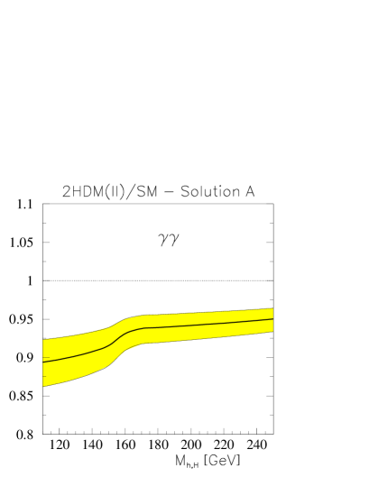
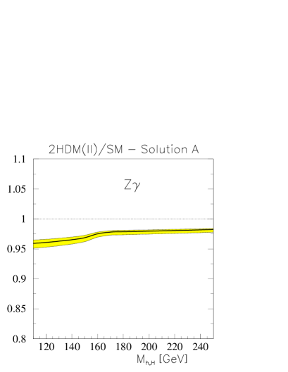
Figure 1: Ratios of the Higgs boson $\phi\to\gamma\gamma$ (left panel) and $\phi\to Z\gamma$ (right panel) decay widths in the 2HDM (II) and the SM as functions of $M_{\phi}$ for all solutions $A$ with $\lambda_{5}=0$. See text for a description of the solid curve and the shaded bands.

Since for these solutions $|\chi_{V}|=1$ with high accuracy and since the $b$-quark contribution is negligible, the uncertainty in the considered loop couplings $|\chi_{a}|^{2}$ (shown as shaded bands) is only due to the uncertainty in $\chi_{u}$ (which enters with the coefficient $k_{\gamma}\approx|[8F_{1/2}(t)/3]|/[F_{1}(W)+4F_{1/2}(t)/3]\approx 32/47\approx 2/3$ at small $M_{h}$ in $R_{\gamma\gamma}$ and a smaller coefficient $k_{Z}$ for $R_{Z\gamma}$). In accordance with the previous discussion, these $k_{\gamma},k_{Z}$ become smaller at higher $M_{h}$. The shaded region above the solid curve corresponds to $\epsilon_{u}>0$ and that below the solid curve to $\epsilon_{u}<0$. In accordance with the discussion in Sec. 5.2, both these regions are relevant to solutions $A_{h+}$ (or $A_{H-}$) and only the lower region is relevant to the solution $A_{h-}$.

6.1.2 The two-gluon width

The two-gluon width is determined by the contributions of the $t$ and $b$ quark loops. For not too high values of $\tan\beta$, the $t$-quark contribution dominates. So, the difference $\chi_{gg}-1$ is determined by the difference $\chi_{u}-1$, and we have checked that with high accuracy $\chi_{gg}-1\approx 2(\chi_{u}-1)=2\epsilon_{u}$. Let us consider now different regions of $\tan\beta$.
(i) If $\tan\beta\ll 1$, then the deviation of the Higgs boson coupling with the $t$-quark from its SM value can be significant, reaching the bounds of the expected experimental uncertainty (3).
(ii) If $\tan\beta>1$, then according to Eq. (13), the deviation of the coupling with the $t$-quark from its SM value should be less than that for the $b$-quark, the latter being constrained from above by the experimental uncertainty (3). Therefore, in this case one expects $|\chi_{gg}-1|<0.05$, which is lower than the expected precision in the measurement of the two-gluon width.

6.2 Solutions B

For solutions $B$ we have, by definition, $\chi_{u}+\chi_{d}={\cal O}(\epsilon)$. So with high accuracy $\chi_{H^{\pm}}\approx\chi_{V}$ (see Eq. (9)), and the final result is independent of $\lambda_{5}$. The results of calculations of photon widths are shown in Fig. 2, where the lower curves correspond to the solutions $B_{\phi\pm d}$ and the upper ones to the solution $B_{h+u}$.

6.2.1 The $\gamma\gamma$ and $Z\gamma$ widths

(i) For the solutions $B_{\phi\pm d}$ the main source of deviation from the SM prediction is due to the charged Higgs contribution and the small change due to the opposite relative sign of the $b$-quark coupling ($\chi_{d}\simeq-\chi_{V}$) as compared to that in the SM case, see Fig. 2, lower curves. Therefore, the lower solid curves in Fig. 2 (calculated for $\chi_{V}=-\chi_{d}=\chi_{u}=\pm 1$) are very close to those for solution $A$ in Fig. 1. Varying the Higgs boson mass $M_{\phi}$ from 110 to 250 GeV we obtain $|\chi_{\gamma\gamma}|^{2}=0.860$ – 0.957 and $|\chi_{Z\gamma}|^{2}=0.953$ – 0.984 for points on the solid curve. The difference from the results for solution $A$ at $\lambda_{5}=0$ is determined mainly by the small $b$-quark loop contribution. Naturally, it decreases for larger values of $M_{\phi}$.

For these solutions the deviation of the $\phi t\bar{t}$ coupling from its SM value is negligible (see Eq. (15)). Besides, since the contribution of the $b$-quark loop is small compared to that of the $t$-quark loop, the photon widths are also insensitive to the experimental uncertainty $\delta_{b}$. The only essential dependence on the experimental inaccuracy is that of $\chi_{V}$. The photonic widths are $\propto(1-\epsilon_{V})^{2}$ with $\epsilon_{V}>0$, so the allowed values of these widths can only be lower than those at $\chi_{V}=\pm 1$. The width of the shaded regions is given by the corresponding factor $1-2\delta_{V}$.

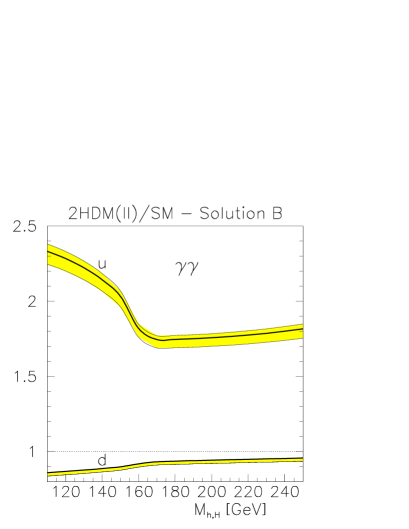
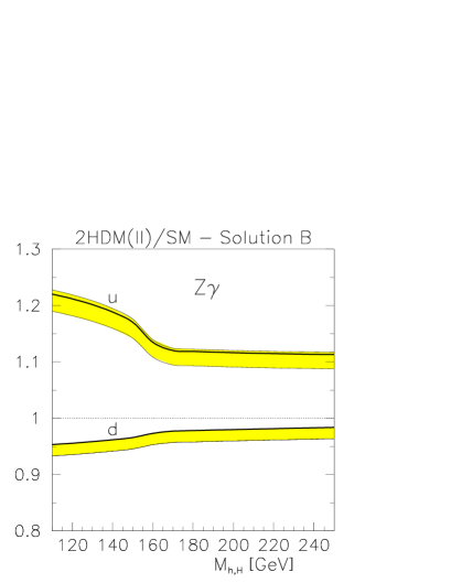
Figure 2: Ratios of the Higgs boson $\phi\to\gamma\gamma$ (left panel) and $\phi\to Z\gamma$ (right panel) decay widths in the 2HDM (II) and the SM as functions of $M_{\phi}$ for all solutions $B$. The lower bands correspond to solutions $B_{\phi\pm d}$. The upper bands correspond to the solution $B_{h+u}$. See the text for a detailed description.

(ii) For the solution $B_{h+u}$ the photon widths change dramatically as compared to the SM case (upper parts in Fig. 2). Here, solid curves correspond to the case $\chi_{V}=\chi_{d}=-\chi_{u}=1$. With the asymptotic values (20) and (21) we obtain $|\chi_{\gamma\gamma}|^{2}\approx(76/47)^{2}\approx 2.6$. The small contribution of the $b$-quark loop decreases this value. The numerical calculation (upper solid curve in Fig. 2) gives here about 2.3 for the ratio of the widths for $M_{h}=110$ GeV. The change of behavior of this curve at $M_{h}\approx 2M_{W}$ corresponds to the change in the $M_{h}$ dependence of the real part, and the onset of the imaginary part of the $W$-loop contribution.

For this solution the experimental uncertainty in the $ht\bar{t}$ coupling becomes essential. The upper shaded regions in the figure are derived numerically from the bounds around the SM values of two measured basic coupling constants, $g_{V}$ ($V=Z$ or $W$) and $g_{u}$ ($=g_{t}$). The first uncertainty, given by $\delta_{Z}$, allows for a reduction of $|\chi_{\gamma\gamma}|^{2}$. The second uncertainty is reduced in the Higgs-two-photon coupling by a factor $k_{\gamma}$ similar to that discussed for solution $A$. In the asymptotic region we have $k_{\gamma}\approx 32/76\approx 0.4$. This reduction factor $k_{\gamma}$ decreases with increasing values of $M_{h}$. It gives the shaded regions, both below and above the solid curve.

6.2.2 The two-gluon width

The two-gluon width has only quark loop contributions. The results of numerical analyses are presented in Fig. 3. The solid curves correspond to the case $\chi_{u}=-\chi_{d}=\pm 1$ for all solutions $B$. As in the asymptotic cases (21), the loop contributions of $t$ and $b$ quarks are of opposite signs and $|F_{1/2}(b)|<|F_{1/2}(t)|$. In the SM case they partly cancel each other, while for solutions $B$ these contributions add. Therefore, for these solutions, the two-gluon width is considerably higher than in the SM. With the asymptotic Eqs. (21) and setting $M_{b}(M_{\phi})=4$ GeV we obtain for $M_{\phi}=110$ GeV the value $|\chi_{gg}|^{2}\approx 1.4$ which is near the value obtained by numerical calculation. Varying the Higgs mass from 110 to 250 GeV we obtain $|\chi_{gg}|^{2}=1.31$ – 1.09.

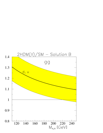
Figure 3: Ratio of the Higgs boson $\phi\to gg$ decay widths in the 2HDM (II) and the SM as function of $M_{\phi}$ for all solutions $B_{\phi\pm d}$ and $B_{h+u}$. The shaded bands correspond to the solution $B_{h+u}$ only (bands above or below the solid curve correspond to $\epsilon_{u}<0$ or $\epsilon_{u}>0$). For the solutions $B_{\phi\pm d}$, the shaded bands are practically reduced to the width of the solid curve.

According to Eq. (15), for the solutions $B_{\phi\pm d}$ the uncertainty in the $\phi t\bar{t}$ coupling is negligible while the uncertainty in the $\phi b\bar{b}$ coupling is suppressed in $\chi_{gg}$ since the $b$-quark loop contribution is small. Therefore, for these solutions $B_{\phi\pm d}$, the shaded bands in the figure are practically degenerated to zero width. However, for the solution $B_{h+u}$, the uncertainty induced by the anticipated 1-$\sigma$ accuracy in the $ht\bar{t}$ coupling is considerable, as indicated by the shaded bands, below and above the solid curve.

6.3 Distinguishing models via loop-induced couplings

Our results for loop-induced couplings show no visible difference in the results between the cases when the observed Higgs boson is the lighter one, $h$, or the heavier one, $H$. Only the (difficult) direct observation of $h$ could in the latter case can rule out this possibility. Taking into account anticipated experimental inaccuracies in the basic couplings of the Higgs boson to fermions, to $Z$ and $W$ bosons and the freedom in the values of $\lambda_{5}$, the discussed experiments cannot discriminate between the solutions $A$ and $B$ either.

The different allowed realizations of an SM-like scenario discussed above, are summarized in Table 3. Note that solutions $A_{h+}$ and $A_{H-}$ are similar in some respects, as are $B_{h+d}$ and $B_{H-d}$. In fact, they lead to the same predictions for the loop-induced couplings, given in Figs. 1, 2 and 3. Each of these solutions corresponds to two regions of $\epsilon_{u}$ ($\epsilon_{d}$), except $A_{h-}$, where only the region $\epsilon_{u}<0$ ($\epsilon_{d}>0$) is allowed. In all these solutions the deviation $\epsilon_{d}$ can be either positive or negative, except for solution $A_{h-}$ for which $\epsilon_{d}$ should be negative.

	$\chi_{V}=g_{V}/g_{V}^{\rm SM}$	$\chi_{d}=g_{d}/g_{d}^{\rm SM}$	$\chi_{u}=g_{u}/g_{u}^{\rm SM}$	$\tan\beta$	$|\chi_{\gamma\gamma}|^{2}$	$|\chi_{Z\gamma}|^{2}$	$|\chi_{gg}|^{2}$
$A_{h+}$	$+(1-\epsilon_{V})$	$+(1-\epsilon_{d})$	$+(1-\epsilon_{u})$	$<1$, $>1$	0.90	0.96	1.00
$A_{h-}$	$-(1-\epsilon_{V})$	$-(1-\epsilon_{d})$	$-(1-\epsilon_{u})$	$\gg 1$	0.90	0.96	1.00
$A_{H-}$	$-(1-\epsilon_{V})$	$-(1-\epsilon_{d})$	$-(1-\epsilon_{u})$	$>1$	0.90	0.96	1.00
$B_{h+d}$	$+(1-\epsilon_{V})$	$-(1-\epsilon_{d})$	$+(1-\epsilon_{u})$	$>1$	0.87	0.96	1.28
$B_{h-d}$	$-(1-\epsilon_{V})$	$+(1-\epsilon_{d})$	$-(1-\epsilon_{u})$	$>1$	0.87	0.96	1.28
$B_{H-d}$	$-(1-\epsilon_{V})$	$+(1-\epsilon_{d})$	$-(1-\epsilon_{u})$	$>1$	0.87	0.96	1.28
$B_{h+u}$	$+(1-\epsilon_{V})$	$+(1-\epsilon_{d})$	$-(1-\epsilon_{u})$	$<1$	2.28	1.21	1.28

Table 3: SM-like scenarios in the 2HDM (II). The solutions correspond to $\epsilon_{V}>0$ and, for each realization, $\epsilon_{d}\epsilon_{u}<0$. The ratios of partial widths (last three columns), refer to the “exact” case ($\epsilon_{i}=0$), for $M_{\phi}=120$ GeV, and $\lambda_{5}=0$.

6.3.1 Distinguishing models at a Photon Collider

Our detailed estimates for loop-induced widths are related to the era after precise measurements of Higgs boson coupling constants at an $e^{+}e^{-}$ Linear Collider with the uncertainties given by Eq. (3).

The comparison of the presented results for the two-photon width with the anticipated experimental uncertainty (4) shows that the deviation of the two-photon width ratio from unity is generally large enough to allow a reliable distinction of the 2HDM (II) from the SM at a Photon Collider. For the solutions $B$ this conclusion is valid for arbitrary values of $\lambda_{5}$ and arbitrary masses of other (unobserved) Higgs bosons. For the solutions $A$, according to Eq. (22), this conclusion is valid in a wide range of $\lambda_{5}$ values, except for the interval (in units of $2\lambda_{4}$) $\sim(1-\delta_{\gamma}/R_{\gamma\gamma},1+\delta_{\gamma}/R_{\gamma\gamma})$. The possible precision in the determination of $\lambda_{5}v^{2}/M^{2}_{H^{\pm}}$ from the two-photon width depends strongly on the achieved precision in the determination of the $ht\bar{t}$ coupling. These conclusions are accurate for a Higgs boson lighter than 140 GeV. A new analysis of experimental uncertainties is necessary if the observed Higgs boson will be heavier than 140 GeV.

The measurement of the $hZ\gamma$ coupling in the process $e\gamma\to eh$ will be an additional test for the considered problems.

6.3.2 Distinguishing models at the Tevatron, LHC and an $e^{+}e^{-}$ Linear Collider

Before a Photon Collider is realized, the SM-like scenario can be considered with respect to data obtained first at the Tevatron, then at the LHC, and finally at an $e^{+}e^{-}$ Linear Collider. The observation of loop-induced couplings can distinguish models in the frame of the “current SM-like scenario” determined via currently measured coupling constants. Even at the Tevatron the solution $B_{h+u}$ can easily be distinguished via a study of the process $gg\to\phi\to\gamma\gamma$ with rate about three times higher than that in the SM (the product of the ratios of decay widths presented in Figs. 3 and 2 (left panel, upper curve)). Such an enhancement is estimated (in some other respect) as observable at the Tevatron [22].

For all other solutions the possibility of distinguishing models before the Photon Collider era is also related to the study of the two-gluon width of the Higgs boson. Unfortunately, the expected experimental precision in the measurement of this quantity is not so high, and the ambiguity in its calculation is also essential. Therefore, the results obtained via the two-gluon width should be supplemented by some independent experiment, such as the two-photon width measured via photon fusion at a Photon Collider.

For all solutions $B_{\phi\pm}$ the two-gluon width is about 30% higher than its SM value at $M_{\phi}=115$ GeV and decreases fast for increasing values of $M_{\phi}$ (due to the change of relative sign of the $t$ and $b$ loop contributions as compared to the SM case). If such a precision can be achieved, it helps to distinguish models via the two-gluon width.

For solutions $A$ the deviation of the two-gluon width in the 2HDM (II) from its SM value is twice as large as the deviation in the Higgs boson coupling to $t$ quarks. The last deviation can be high if $\tan\beta\ll 1$. In this case it can happen that the deviation of the two-gluon width from its SM value will be observable while the deviation in the coupling to $t$ quarks will lie below the experimental resolution. Note that the possible decrease of the two-gluon width as compared to the SM value can be realized only in solutions $A$. (The value $|\chi_{gg}|^{2}>1$ can be realized in both solutions $A$ and $B$.)

6.4 Distinguishing the MSSM from the SM

In a forthcoming publication we plan to study the MSSM in this same SM-like scenario. In this model only some of the solutions $A$ of the pattern relation can be realized, and the additional constraint on $\lambda_{5}$ ($\approx 2\lambda_{4}$) makes the contribution of the charged Higgs boson to the discussed photon width very small. On the other hand, the contributions of superpartners can be substantial. Since the mechanism of generation of their masses differs from that in the SM, superparticles are completely decoupled from the Higgs boson if they are sufficiently heavy.

The question whether or not it is possible to see signals of the MSSM as compared to the SM in this decoupling limit, was considered in Ref. [5]. The two-photon width was studied for finite values of superparticle masses, but using an old estimate for the uncertainty in BR$(h\to\gamma\gamma)$, 10%, instead of the modern value (4). With that uncertainty, it was concluded that the MSSM and the SM cannot be resolved via the two-photon width even for light chargino and top squark (250 GeV). These estimates should be reconsidered to obtain real bounds, relevant to the uncertainty (4). Also, one should consider masses of superpartners and other parameters of the theory at which the models cannot be distinguished in other ways. Such values could be above the discovery limits for the LHC.

7 Conclusion

We consider the case that after the Higgs boson discovery no signal of New Physics will be found (SM-like scenario). This can occur both in the SM and in other models, including the 2HDM (II), MSSM, etc. Realization of an SM-like scenario constrains these alternative models strongly, and measurements of loop-induced couplings of the observed Higgs boson can help to understand which model is realized.

In this paper we consider this problem in the 2HDM (II) for a Higgs boson (which can be either one of two neutral scalars, $h$ or $H$). For this purpose, we consider the ratios of measurable couplings of the Higgs boson with quarks and electroweak gauge bosons to their SM values. We obtain constraints on the 2HDM (II) in the form of a pattern relation among these ratios. (These particular pattern relations are valid also in the MSSM.)

We analyzed two possible classes of solutions of the pattern relation for the considered SM-like scenario. In the solutions $A$ all basic couplings are close to their SM values. In the solutions $B$ some of the basic couplings are close to their SM values while others differ in sign from the SM values. Next, we calculated the $\gamma\gamma$ and $Z\gamma$ partial widths of the observed Higgs boson for all considered solutions, taking into account anticipated uncertainties in future measurements of the basic couplings of the Higgs boson.

The results of our calculations are shown in the figures. The solid curves describe an “exact” SM-like scenario with basic couplings $\chi_{i}=\pm 1$. The shaded bands represent effects of experimental uncertainties in the measurement of basic couplings at an $e^{+}e^{-}$ Linear Collider for $M_{\phi}<140$ GeV (3).

If $M_{\phi}>140$ GeV, these estimates of shaded bands should be reconsidered. In this region the dominant decay channels of SM-like Higgs boson changes (becoming $WW^{*}$ and $ZZ^{*}$) just as the main mechanism of its production at an $e^{+}e^{-}$ collider changes ($W$ fusion instead of Higgs-strahlung). Therefore, the values of the uncertainties of couplings of the Higgs boson to quarks, $W$ and $Z$ will be changed.

Our main results are related to the era after the LHC and $e^{+}e^{-}$ Linear Collider operations if the SM-like scenario will be found to be realized at that time. We found the difference between the SM and the 2HDM (II) to be large enough to discriminate the models via measurements of Higgs boson production at a Photon Collider — for solutions $B$ in general, and for solutions $A$ except a limited range of values of $\lambda_{5}$.

For the period of operations at the Tevatron, LHC and an $e^{+}e^{-}$ Linear Collider we obtain the regions in the parameter space where the basic couplings squared are close to the SM case but the loop-induced two-gluon or two-photon widths differ so significantly from their SM values that one can distinguish the 2HDM (II) from the SM via experiments at the LHC or at an $e^{+}e^{-}$ Linear Collider.

We are grateful to A. Djouadi, J. Gunion, H. Haber and M. Spira for discussions of decoupling in the 2HDM and the MSSM, and to P. Chankowski, W. Hollik and I. Ivanov for valuable discussions of the parameters of the 2HDM. MK is grateful to the University of Bergen and to the Theory Group at DESY for warm hospitality and financial support. This research has been supported by RFBR grants 99-02-17211 and 00-15-96691, by Polish Committee for Scientific Research, grant No. 2P03B01414, and by the Research Council of Norway.

References

- [1] I.F. Ginzburg, G.L. Kotkin, V.G. Serbo, V.I. Telnov, Nucl. Instrum. Methods 205, 47 (1983); I.F. Ginzburg, G.L. Kotkin, S.L. Panfil, V.G. Serbo, V.I. Telnov, Nucl. Instrum. Methods, A 219, 5 (1984); Zeroth-order Design Report for the NLC, SLAC Report 474 (1996); R. Brinkmann et al., Nucl. Instrum. Methods, A 406, 13 (1998).
- [2] E. Accomando et al., Phys. Rept. 299, 1 (1998).
- [3] I.F. Ginzburg, M. Krawczyk, P. Osland, Proc. 4th Int. Workshop on Linear Colliders, April 28-May 5, 1999; Sitges (Spain) p. 524, (hep-ph/9909455); I.F. Ginzburg, Nucl. Phys. B (Proc. Suppl.) 82, 367 (2000); hep-ph/9907549.
- [4] H.E. Haber, Talk given at Beyond the Standard Model Conf., Lake Tahoe, CA, Dec. 13-18, 1994 and at Ringsberg Workshop on Perspectives for Electroweak Interactions in Collisions, Ringsberg, Germany, 5-8 Feb. 1995, hep-ph/9505240; in Perspectives on Higgs Physics II, Gordon L. Kane ed., World Scientific, Singapore, 1997, hep-ph/9707213.
- [5] A. Djouadi, V. Driesen, W. Hollik, J.I. Illana, Eur. Phys. J. C 1, 149 (1998); A. Djouadi, V. Driesen, W. Hollik, A. Kraft, Eur. Phys. J. C 1, 163 (1998).
-
[6]
R. Barate et al. [ALEPH Collaboration],
Phys. Lett. B495, 1 (2000)
[hep-ex/0011045];
M. Acciarri et al. [L3 Collaboration], hep-ex/0012019. -
[7]
See e.g., A. Djouadi et al. (Higgs working group), Workshop on
Physics at TeV Colliders, Les Houches, France, June 1999,
hep-ph/0002258;
ATLAS detector and Physical Performance Technical Design Report,
http://atlasinfo.cern.ch/Atlas/GROUPS/PHYSICS/TDR/access.html,
G. L. Bayatian et al., CMS Technical Proposal, CERN LHCC 94-38 (1994),
http://cmsinfo.cern.ch/TP/TP.html; D. Zeppenfeld, hep-ph/0005151. - [8] See TESLA Technical Design Report, to be published. Previous estimates can be found in M. Battaglia, Proc. 4th Int. Workshop on Linear Colliders, April 28-May 5, 1999; Sitges (Spain), hep-ph/9910271; A. Djouadi, ibid., hep-ph/9910449; P. Zerwas, hep-ph/0003221.
- [9] K. Hagiwara, S. Ishihara, J. Kamoshita and B. A. Kniehl, Eur. Phys. J. C14, 457 (2000) [hep-ph/0002043].
- [10] M. Battaglia and K. Desch, hep-ph/0101165.
- [11] V.I. Telnov, Talk given at International Workshop on High-Energy Photon Colliders, Hamburg, Germany, 14–17 June 2000, to be published in Nucl. Instrum. Meth.; hep-ex/0012047.
- [12] M. Melles, W.J. Stirling, V.A. Khoze, Phys. Rev. D 61, 054015 (2000); G. Jikia, S. Söldner-Rembold, Nucl. Phys. B (Proc. Suppl.) 82, 373 (2000).
- [13] J.F. Gunion, H.E. Haber, G. Kane, S. Dawson, The Higgs Hunter’s Guide (Addison-Wesley, Reading, 1990).
- [14] R. Santos and A. Barroso, Phys. Rev. D 56, 5366 (1997).
- [15] M. Krawczyk, in Proceedings of the 28th International Conference on High Energy Physics, ICHEP ’96, editors Z. Ajduk and A.K. Wroblewski (World Scientific, Singapore, 1997) p. 1460; M. Krawczyk and J. Żochowski, Phys. Rev. D 55, 6968 (1997); M. Krawczyk, J. Żochowski, P. Mattig, Eur. Phys. J. C 8, 495 (1999); P.H. Chankowski, M. Krawczyk, J. Żochowski, Eur. Phys. J. C 11, 661 (1999); M. Krawczyk, P. Mattig, J. Żochowski, Eur. Phys. J. C in press, hep-ph/0009201.
- [16] B. Grza̧dkowski, J.F. Gunion, J. Kalinowski, Phys. Rev. D 60, 075011 (1999); Phys. Lett. B 480, 287 (2000).
- [17] S. Heinemeyer, W. Hollik and G. Weiglein, Eur. Phys. J. C 9, 343 (1999).
- [18] P. Chankowski et al., hep-ph/0009271, Phys. Lett. B, to appear.
- [19] L. Resnick, M.K. Sundaresan and P.J.S. Watson, Phys. Rev. D 8, 172 (1973); J. Ellis, M.K. Gaillard and D.V. Nanopoulos, Nucl. Phys. B106, 292 (1976); A.I. Vainshtein, M.B. Voloshin, V.I. Zakharov and M.A. Shifman, Sov. J. Nucl. Phys. 30, 711 (1979).
-
[20]
V. Barger, J. L. Hewett and R. J. Phillips,
Phys. Rev. D 41, 3421 (1990);
Y. Grossman, Nucl. Phys. B426, 355 (1994) [hep-ph/9401311]. - [21] A. T. Banin, I. F. Ginzburg and I. P. Ivanov, Phys. Rev. D 59, 115001 (1999) [hep-ph/9806515].
- [22] S. Mrenna and J. Wells, Phys. Rev. D 63, 015006 (2001) [hep-ph/0001226].