Solar neutrino problem accounting for self-consistent magnetohydrodynamics solution for solar magnetic fields

Abstract

The analysis of the resonant spin–flavour (RSF) solutions to the solar neutrino problem in the framework of simplest analytic solutions to the solar magneto-hydrodynamics (MHD) equations is presented. We performed the global fit of the recent solar neutrino data, including event rates as well as day and night recoil electron spectra induced by solar neutrino interactions in SuperKamiokande. We compare quantitatively our simplest MHD-RSF fit with vacuum oscillation (VAC) and MSW–type (SMA, LMA and LOW) solutions to the solar neutrino problem using a common well–calibrated theoretical calculation and fit procedure and find MHD-RSF fit to be somewhat better than those obtained for the favored neutrino oscillation solutions. We made the predictions for future experiments to disentangle the MHD-RSF scenario from other scenarios.

1 Introduction

The problem of disagreement between solar neutrino data and theoretical expectations has been a long-standing problem in physics. The most popular solutions of the solar neutrino anomalies have as a basis the idea of neutrino oscillations, either in vacuum or in the Sun due to the enhancement arising from matter effects [1]. There are alternative interpretations the problem. Here we will re-analyze the status of resonant spin–flavour solutions [2, 3] to the solar neutrino problem in the light of the most recent global set of solar neutrino data. In contrast to previous attempts [2, 3, 4] we will adopt the general framework of self–consistent magneto–hydrodynamic (MHD) models of the Sun [5]. For definiteness we will concentrate in the recent proposal of Ref. [6]. We perform global fits of solar neutrino data for realistic solutions to the magneto-hydrodynamics equations inside the Sun. This way and by neglecting neutrino mixing we obtain the simplest MHD-RSF solution to the solar neutrino problem, characterized by two effective parameters, $\Delta m^{2}$ and $\mu_{\nu}B_{\perp max}$, $B_{\perp max}$ being the maximum magnitude of the magnetic field inside the convective region. We find that our simplest two-parameter MHD-RSF fits to the solar neutrino data are slightly better than those for the oscillation solutions. The required best fit points correspond to maximum magnetic field magnitudes in the convective zone smaller than 100 KG. We briefly discuss the prospects to distinguish our simplest MHD-RSF scenario from the neutrino oscillation solutions to the solar neutrino problem.

2 Static Magnetic Field Profiles in the Sun

In solar magneto-hydrodynamics [7] (MHD, for short) the corresponding magnetic field profiles are rather complicated and difficult to extract. However, there are stationary solutions which are known analytically in terms of relatively simple functions [6].

We consider the magnetic field profile which are only solutions to the equation for a static MHD plasma configuration in a gravitational field, given by

$$\nabla p-\frac{1}{c}\vec{j}\times\vec{B}+\rho\nabla\Phi=0.$$ (1)

This static MHD equations correspond to a quiet Sun and they admit axially symmetric solutions in the spherically symmetric gravitational field which can be simply expressed in terms of spherical Bessel functions and were first discussed in Ref. [6]. The model magnetic field depends on $z_{k}$, the roots of the spherical Bessel function $f_{5/2}=\sqrt{z}J_{5/2}(z)$. Taking into account the boundary condition that $\vec{B}$ vanishes on the solar surface the magnetic field have the analytical form

$$B^{k}_{r}(r,\theta)=2\hat{B}^{k}\cos\theta$$

$$\hfill\times\left[1-\frac{3}{r^{2}z_{k}\sin z_{k}}\left(\frac{\sin(z_{k}r)}{z_{k}r}-\cos(z_{k}r)\right)\right]~{},$$

$$B^{k}_{\theta}(r,\theta)=-\hat{B}^{k}\sin\theta$$

$$\times\left[2+\frac{3}{r^{2}z_{k}\sin z_{k}}\left(\frac{\sin(z_{k}r)}{z_{k}r}-\right.\right.$$

$$\biggl{.}\biggl{.}-\cos(z_{k}r)-z_{k}r\sin(z_{k}r)\biggr{)}\biggr{]}~{},$$

$$B^{k}_{\phi}(r,\theta)=\hat{B}^{k}z_{k}\sin\theta$$

$$\times\left[r-\frac{3}{rz_{k}\sin z_{k}}\left(\frac{\sin(z_{k}r)}{z_{k}r}-\cos(z_{k}r)\right)\right]~{},$$ (2)

where the coefficient $\hat{B}^{k}(B_{core})$ is given by

$$\hat{B}^{k}=\frac{B_{core}}{2(1-z_{k}/\sin z_{k})}~{}.$$ (3)

The distance $r$ has been normalized to $R_{\odot}=1$. In our calculations we have averaged over polar angle $\theta$.

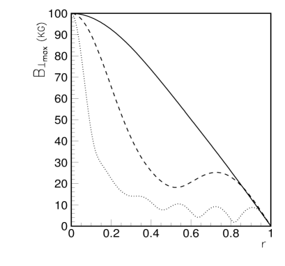
Figure 1: The perpendicular component of B for various $k$–values 1 (solid), 3 (dashed) and 10 (dotted).

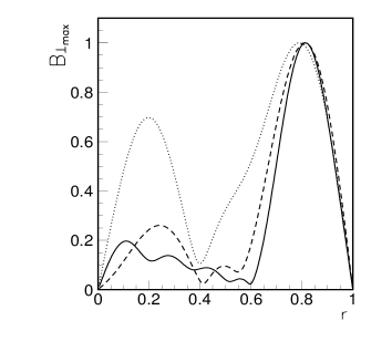
Figure 2: Magnetic field configurations obtained by combining individual modes for different $k_{M}$ values, 5, 6 and 10 (dotted, dashed and solid). Summing up to higher modes achieves better localization of the field in the convective region (solid).

Parameter $B_{core}$ is a central magnetic field. In Fig. 1 we display the perpendicular component of B for various $k$–values 1, 3 and 10, which correspond to the roots $z_{1}=5.7$, $z_{3}=12.3$ and $z_{10}=34.5$, respectively.

We have to discuss the astrophysical restrictions on the free parameters $B_{core}$ and $k$ characterizing the model. The magnitude of a magnetic field at the center of the Sun is constrained by the Fermi-Chandrasekhar limit [8] which requires an upper bound on $B_{core}\;\raise 1.29167pt\hbox{$<$\kern-7.5pt\raise-4.73611pt\hbox{$\sim$}}\;2~{}$ MGauss.

The possible values of $k$ can be constrained by taking into account that in order to justify the use of a stationary solution, it is necessary that the diffusion time due to ohmic dissipation must be less than solar life time. The simple estimations give us that reasonable values of $k$ are less $10$. It is commonly accepted that magnetic fields measured at the surface of the Sun are weaker than within the convective zone interior where this field is supposed to be generated. On the other hand the general knowledge of the solar magnetic field models is that the magnetic field increases at the overshoot layer, while being small at the solar interior, a picture rather opposite to the one we have seen in Fig. 1. The correct way is to use the linear nature of the basic equilibrium MHD equation in eq. (1). This implies that any linear combination of solutions $\vec{B}^{k}$ ($k=1,2,\dots,k_{M}$, for some fixed number $k_{M}<10$) $\vec{B}=c_{1}\vec{B_{1}}+c_{2}\vec{B_{2}}+...+c_{M}\vec{B_{M}}$ is also a solution. We will require that combined magnetic field is equal to zero in the center of the Sun and it’s total energy must be minimal in the region below the bottom of the convective zone, characterized by a certain value of $r_{0}$.

The procedure sketched above provides a consistent method for combining individual mode solutions $\vec{B_{k}}$ of the static MHD equation (Fig. 2).

Table 1: Solar neutrino rates measured in the Chlorine, Gallium and Super–Kamiokande experiments.

Experiment	Rate	Ref.	Units	$R^{\rm BP2000}_{i}$
Homestake	$2.56\pm 0.23$	[11]	SNU	$7.8\pm 1.1$
GALLEX+GNO+SAGE	$74.66\pm 5.2$	[12, 13, 14]	SNU	$130\pm 7$
Super–Kamiokande	$2.40\pm 0.08$	[16]	$10^{6}$ cm${}^{-}2$ s-1	$5.2\pm 0.9$

3 Fitting the Solar Neutrino Data

We will neglect neutrino mixing and consider the case of active-active neutrino conversions. In this case the $\nu_{e}\to\bar{\nu}_{\ell}$ conversions are described by the master Schrödinger evolution equation

$$i\left(\begin{array}[]{l}\dot{\nu}_{e}\\ \dot{\bar{\nu}_{\ell}}\\ \end{array}\right)=\left(\begin{array}[]{cc}V_{e}-\delta&\mu_{\nu}B_{+}\\ \mu_{\nu}B_{-}&-V_{\ell}+\delta\\ \end{array}\right)\left(\begin{array}[]{c}\nu_{e}\\ \bar{\nu}_{\ell}\\ \end{array}\right)~{},$$ (4)

where $\mu_{\nu}$ denotes the neutrino transition magnetic moment [9] in units of $10^{-11}$ $\mu_{B}$, $\ell$ denoting either $\mu$ or $\tau$. Here $B_{\pm}=B_{x}\pm iB_{y}$ and $\delta=\Delta m^{2}/4E$ is the neutrino mass parameter; $V_{e}(t)=G_{F}\sqrt{2}(\rho(t)/m_{p})(Y_{e}-Y_{n}/2)$ and $V_{\ell}(t)=G_{F}\sqrt{2}(\rho(t)/m_{p})(-Y_{n}/2)$ are the neutrino vector potentials for $\nu_{e}$ and $\nu_{\ell}$ in the Sun given by the abundances of the electron ($Y_{e}=m_{p}N_{e}(t)/\rho(t)$) and neutron ($Y_{n}=m_{p}N_{n}(t)/\rho(t)$) components. In our numerical study of solar neutrino data we adopt the Standard Solar Model density profile of ref.[10].

We solve Eq. (4) numerically by finding a solution of the Cauchy problem in the form of a set of wave functions $\nu_{a}(t)=\mid\nu_{a}(t)\mid e^{i\Phi_{a}(t)}$ from which the neutrino survival probabilities $P_{aa}(t)=\nu_{a}^{*}\nu_{a}$ are calculated. They obey the unitarity condition $\sum_{a}P_{aa}=1$ where the subscript $a$ denotes $a=e$ for $\nu_{e}$ and $a=\ell$ for $\bar{\nu}_{\ell}$ respectively.

The typical neutrino survival probability $P_{ee}$ calculated in the MHD-RSF scheme from eq. (4) plotted versus $E/\Delta m^{2}$ in Fig. 3.

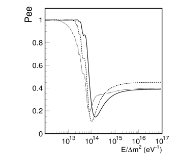
Figure 3: Typical MHD-RSF neutrino survival probability $P_{ee}$ versus $E/\Delta m^{2}$.

We determine the allowed range of oscillation parameters using the total event rates of the Chlorine [11], Gallium [12, 13, 14] and Super–Kamiokande [15, 16] (corresponding to the 1117 days data sample) experiments. For the Gallium experiments we have used the weighted average of the results from GALLEX+GNO and SAGE detectors (see Table 1). We have also included the Super–Kamiokande electron recoil energy spectrum measured separately during the day and night periods. For details on the statistical analysis applied to the different observable we refer to Ref. [17].

We have found that allowed regions of neutrino parameters are pretty stable and does not depend significantly on the choice of $k_{M}$ and $r_{0}$ allowed by astrophysics. In Fig. 4 we display the region of MHD-RSF parameters allowed by the solar neutrino rates for the case $k_{M}=6$ and $r_{0}=0.6R\odot$. We can see that there are several allowed regions for different values of the magnetic field.

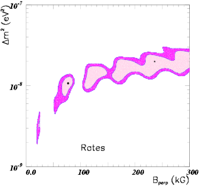
Figure 4: MHD-RSF 90% CL (light) and 99% CL (dark) regions of $\Delta m^{2}$ versus $B_{\perp max}$(KG) allowed by the rates given in table 1, for $r_{0}=0.6$ and $k_{M}=6$.

Apart from total event rates the water Cerenkov experiment also measures the zenith angle distribution of solar neutrino events as well as their electron recoil energy spectrum with their recent 1117-day data sample [16]. The predicted spectrum is essentially flat except for the upper part of the $\Delta m^{2}$ region. As an example, we show in Fig.5 the excluded region at 99 % CL for the case $k_{M}=6$ and $r_{0}=0.6$.

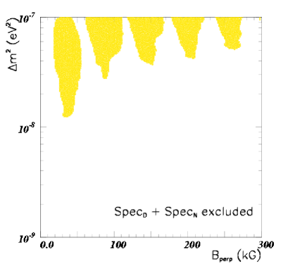
Figure 5: MHD-RSF 99% CL regions of $\Delta m^{2}$ versus $B_{\perp max}$ forbidden by the recoil electron spectrum data for $r_{0}=0.6$ and $k_{M}=6$.

For this reason, the allowed regions are slightly modified by the inclusion of the energy spectrum data for the day and night periods. In Fig. 6 we have presented the results of global fit analysis.

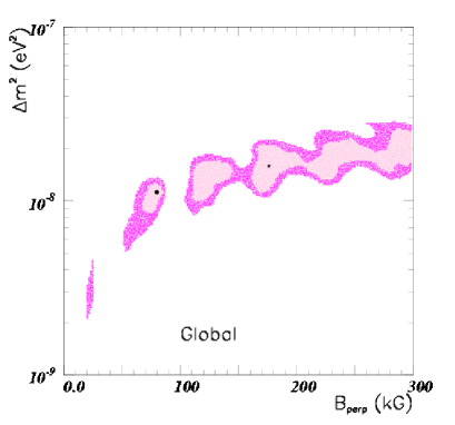
Figure 6: MHD-RSF 90% CL (light) and 99% CL (dark) regions of $\Delta m^{2}$ versus $B_{\perp max}$(KG) allowed by the global solar neutrino fit, for $r_{0}=0.6$ and $k_{M}=6$.

In the case of active-sterile MHD-RSF conversions we obtain that. the rates fit $\chi_{rates}^{2}$ is worse than for the active-active case.

4 Discussion & Conclusions

Figure 7: Neutral-to-charged-current event ratio expected at SNO for different solutions to the solar neutrino problem at 90% CL and 99% CL. The no-oscillation or SM case is denoted by the horizontal line at one.

Table 2: Best fit points and the corresponding probabilities for different solutions to the solar neutrino problem [17]. The top row corresponds to the MHD-RSF solution presented here.

Solution	$\Delta m^{2}$	$B_{\perp{max}}$	$\chi^{2}_{min}$ (Prob %)
$MHD-RSF_{a}$	$1.1\times 10^{-8}$	80	30.4 (73)	This work
$MHD-RSF_{s}$	$1.1\times 10^{-8}$	77	34.9 (52)
	$\Delta m^{2}$	$\sin^{2}(2\vartheta)$	$\chi^{2}_{min}$ (Prob %)	Ref.
$SMA_{a}$	$5.0\times 10^{-6}$	$2.2\times 10^{-3}$	38.9 (34)	[17]
LMA	$3.2\times 10^{-5}$	0.75	33.4 (59)	[17]
LOW	$1.0\times 10^{-7}$	0.93	37.4 (40)	[17]
QVO	$2.3\times 10^{-9}$	0.96(d)	40.3 (29)	[17]
VAC	$6.7\times 10^{-10}$	0.93(d)	39.3 (32)	[17]
$SMA_{s}$	$3.9\times 10^{-6}$	$2.4\times 10^{-3}$	39.6 (31)	[17]
no-osc			91 ($3\times 10^{-4}$)	[17]

From the results of the previous section it follows that our MHD-RSF solution to the solar neutrino problem provides a good description of the most recent solar neutrino data, including event rates as well as zenith angle distributions and recoil electron spectra induced by solar neutrino interactions in Superkamiokande. We have shown that our procedure is quite robust in the sense that the magnetic field profile has been determined in an essentially unique way. This effectively substitutes the neutrino mixing which characterizes the oscillation solutions by a single parameter $B_{\perp max}$ characterizing the maximum magnitude of the magnetic field inside the convective region. The value of $k_{M}$ characterizing the maximum number of individual modes superimposed in order to obtain a realistic profile and the parameter $r_{0}$ characterizing the location of the convective region are severely restricted. The allowed $k_{M}$ values are restricted by ohmic dissipation arguments to be lower than 10 or so, while $r_{0}$ is close to $0.6R_{\odot}$. We have found that our solar neutrino fits are pretty stable as long as $k_{M}$ exceeds 5 and $r_{0}$ lies in the relevant narrow range. Therefore our fits are effectively two–parameter fits ($\Delta m^{2}$ and $B_{\perp max}$) whose quality can be meaningfully compared with that of the fits obtained for the favored neutrino oscillation solutions to the solar neutrino problem.

In table 2 we compare the various solutions of the solar neutrino problem with the MHD-RSF solutions for the lower magnetic field presented here.

Clearly the MHD-RSF fits seem somewhat better (though not in a statistically significant way) than those obtained for the MSW effect  [17] as well as just–so solutions [18].

We determined the expected solar neutrino rates at SNO within the framework of our MHD-RSF solution to the solar neutrino problem. We used the cross sections of the CC and NC $\nu d$ reactions given by ref. [19] and the best–fit points we have determined in the present paper. For definiteness we have considered the global best fit points and local minima for $B_{\perp{max}}<100$ KG for the case $k_{M}=6$ and $r_{0}=0.6$ and active-active MHD-RSF conversions.

We have calculated the neutral-to-charged-current event ratio (NC/CC for short) and our results are presented in Fig. 7.

Clearly from Fig. 7 we see that there is a substantial overlap between our MHD-RSF predictions and those found for each of the oscillation solutions (SMA, LMA, LOW, VAC). The overlap is especially large between the LMA and the MHD-RSF solutions. Taking into account the present theoretical uncertainties and a reasonable estimate of the experimental errors attainable, it follows that an unambiguous discrimination between our MHD-RSF solution and the neutrino oscillation–type solutions to the solar neutrino problem on the basis of the averaged event rates seems rather difficult.

Acknowledgments

We thank Alexei Bykov, Vladimir Kutvitsky, Dmitri Sokoloff and Victor Popov for useful discussions. This work was supported by Spanish DGICYT grant PB98-0693, by the European Commission TMR networks ERBFMRXCT960090 and HPRN-CT-2000-00148, by the European Science Foundation network N. 86 and by Iberdrola grant. VBS and TIR were partially supported by the RFBR grant 00-02-16271. OGM was supported by the CONACyT-Mexico grant J32220-E. TIR participation in the Conference was supported by the INTAS-ESF grant 00-36. TIR especially thanks the Organizing Committee of the Conference for the warm and friendly atmosphere.

References

-
[1]
S.P. Mikheev, A.Yu. Smirnov, Sov. J. Nucl. Phys. 42
(1985) 913;
Nuovo Cimento C9 (1986) 17; L. Wolfenstein, Phys. Rev. D17 (1978) 2369. - [2] C. Azneziris and J. Schechter, Phys. Rev. D45 (1992) 1053; C. Azneziris and J. Schechter, IJMP, A6 (1991) 2375; E. Kh. Akhmedov, S. T. Petcov and A. Yu. Smirnov, Phys. Rev. D48 (1993) 2167; A. B. Balantekin ahd F. Loreti, Phys. Rev. D48 (1993) 5496; T. Kubota, T. Kurimoto, M. Osura, E. Takasugi, Phys. Lett. B292 (1992) 195.
- [3] E. Kh. Akhmedov, Phys. Lett. B 213 (1988) 64; C.-S. Lim and W.J. Marciano, Phys. Rev. D 37 (1988) 1368.
- [4] M.M. Guzzo and H. Nunokawa, Astropart. Phys. 11 (1999) 317; J. Pulido, E.K. Akhmedov, hep-ph/9907399; E. K. Akhmedov and J. Pulido, hep-ph/0005173; J. Derkaoui, Y. Tayalati, hep-ph/9909512.
- [5] H. Yoshimura, Astrophys. J., 178 (1972) 863; Astrophys. J. Suppl. Ser., 52 (1983) 363; M. Stix, Astron. & Astrophys. 47 (1976) 243; Ya. B. Zeldovich, A. A. Ruzmaikin and D.D. Sokoloff, Magnetic Fields in Astrophysics, Gordon and Breach Science Publishers, 1983 and references therein.
- [6] V. A. Kutvitskii, L.S. Solov’ev, JETP, 78 (1994) 456.
- [7] E.N. Parker, Cosmological Magnetic Fields, Oxford University Press, Oxford, 1979; E.N. Parker, Astrophys. J., 408 (1993) 707.
- [8] S. Chandrasekar and E. Fermi, Astrophys. J., 118 (1953) 116.
- [9] J. Schechter and J. W. F. Valle, Phys. Rev. D24 (1981) 1883; Erratum-ibid. D25 (1982) 283.
- [10] J.N. Bahcall, S. Basu and M. Pinsonneault, astro-ph/0010346; Bahcall’s Home Page, http://www.sns.ias.edu/jnb/SNdata
- [11] B. T. Cleveland et al., Astrophys. J. 496, 505 (1998); R. Davis, Prog. Part. Nucl. Phys. 32, 13 (1994).
- [12] GALLEX Collaboration, W. Hampel et al., Phys. Lett. B447, 127 (1999).
- [13] Talk by E. Belloti at Neutrino 2000, Sudbury, Canada, June 2000 (http://nu2000.sno.laurentian.ca).
- [14] SAGE Collaboration, J. N. Abdurashitov et al., Phys. Rev. C60, 055801 (1999); Talk by V. Gavrin at Neutrino 2000, Sudbury, Canada, June 2000 (http://nu2000.sno.laurentian.ca).
- [15] Super–Kamiokande Collaboration, Y. Fukuda et al., Phys. Rev. Lett. 81, 1158 (1998); Erratum 81, 4279 (1998); 82, 1810 (1999); 82, 2430 (1999); Y. Suzuki, Nucl. Phys. B (Proc. Suppl.) 77, 35 (1999).
- [16] Talk by Y. Suzuki at Neutrino 2000, Sudbury, Canada, June 2000 (http://nu2000.sno.laurentian.ca).
- [17] M. C. Gonzalez-Garcia, P. C. de Holanda, C. Pena-Garay and J. W. F. Valle, Nucl. Phys. B573 (2000) 3 [hep-ph/9906469]; M. C. Gonzalez-Garcia and C. Pena-Garay, hep-ph/0009041.
- [18] C. Giunti, M. C. Gonzalez-Garcia and C. Pena-Garay, Phys. Rev. D62 (2000) 13005 [hep-ph/0001101].
- [19] K. Kubodera, S. Nozawa, Int. J. Mod. Phys. E 3 (1994) 101; K. Kubodera’s homepage, http://nuc003.psc.sc.edu/kubodera/.