DEEP INELASTIC SCATTERING OF LEPTONS
AND HADRONS IN THE QCD PARTON MODEL
AND EXPERIMENTAL TESTS

Abstract

We present the basic aspects of deep inelastic phenomena in the framework of the QCD parton model. After recalling briefly the standard kinematics, we discuss the physical interpretation of unpolarized and polarized structure functions in terms of parton distributions together with several important sum rules. We also make a rapid survey of the experimental situation together with phenomenological tests, in particular concerning various QCD predictions. In the summary, we try to identify some significant open questions, to clarify where we stand and to see what we expect to learn in the future.

I Introduction

The deep inelastic phenomena has been extensively studied, for about a quarter of a century, both theoretically and experimentally. The main purposes of this vast physics programme were, first to elucidate the internal structure of the nucleon and later on, to test perturbative Quantum Chromodynamics (QCD) which generalizes the parton model. At the end of the sixties, the first measurements on charged lepton deep inelastic scattering (DIS) at the Stanford Linear Accelerator (SLAC) have shown that the nucleon is made of hard point-like objects[1], which was the first evidence for the existence of sub-nuclear particles called partons[2]. Unlike the $ep$ elastic scattering cross section which drops very rapidly for large momentum transfer, the observed cross sections for $eN\to e^{\prime}X$ were much larger than expected, when the off-shell photon probing the nucleon had a large $Q^{2}$. Actually these cross sections were $Q^{2}$ independent and they obeyed the scaling behavior predicted by Bjorken[2], whose physical picture was first given by Feynman[3], in terms of the quark parton model (QPM). The explanation of scaling was based on the fact that a hard collision among partons takes place in such a short time, so that partons behave as if they were free objects. This significant observation led to the consideration of non-Abelian gauge field theories, which possess the crucial property of asymptotic freedom, and to propose QCD as the fundamental theory for strong interactions[4]. It is now well established that QCD is an asymptotically free theory and the strong interaction coupling $\alpha_{s}(Q^{2})$ becomes small when $Q^{2}$ is large, i.e. at short distances. However scale invariance is broken because of quantum corrections and therefore one expects scaling violations which are calculable in perturbative QCD.

The outline of this chapter is as follows. In section II we discuss the kinematics of DIS and define the relevant structure functions for both unpolarized and polarized cases. We provide the physical interpretation of the structure functions in terms of quark parton distributions in section III. We also give their main features from some recent data on unpolarized and polarized structure functions and we recall several important sum rules. In section IV we go briefly one step beyond the QPM to consider scaling violations and to make phenomenological tests. Finally in section V, we give a short summary on significant open questions, and we try to clarify where we stand and what we expect to learn in the future.

II Kinematics of DIS and structure functions

A $ep\to e^{\prime}X$ unpolarized case

Let us start to recall the basic kinematics entering in the calculation of the cross section for the DIS process $ep\to e^{\prime}X$ to lowest order in Quantum Electrodynamics (QED), as shown in Fig. 1. We define the Lorentz invariants in the usual way

$$s = (p+k)^{2},\quad q^{2}=(k-k^{\prime})^{2}=-Q^{2}(Q^{2}>0),$$ (1)

$$\nu = pq/M,\quad W^{2}=p^{\prime 2}=M^{2}+2M\nu-Q^{2},$$ (2)

where $M$ is the proton mass and we neglect the lepton mass. In the laboratory frame, if $E$ and $E^{\prime}$ are the energies of the incoming and outgoing leptons and $\theta$ is the scattering angle one has

$$Q^{2}=4EE^{\prime}\sin^{2}\theta/2\quad\hbox{and}\quad\nu=E-E^{\prime},$$ (3)

which are the invariant mass and the energy of the exchange off-shell photon. One also defines two dimensionless scaling variables

$$x=Q^{2}/2p.q=Q^{2}/2M\nu\quad\hbox{and}\quad y=p.q/p.k=\nu/E,$$ (4)

which can vary between zero and one. We recall that $x$ is called the Bjorken variable and we note that $x=1$ corresponds to elastic $ep$ scattering, since from eq.(2), if $W^{2}=M^{2}$ one has $Q^{2}=2M\nu$. Moreover for $x=0$, i.e. $Q^{2}=0$, we have real photoproduction. Let us recall that DIS corresponds to the ideal situation where $x$ is fixed and $Q^{2}$ and $\nu$ are going to infinity, which is never achieved in practice.

FIG. 1.: The basic Feynman diagram for deep inelastic electron proton scattering in lowest order QED. The final hadron state which is not measured is denoted by $X$.

The unpolarized cross section described by the Feynman diagram shown in Fig. 1 has the following expression

$$\frac{d^{2}\sigma}{dE^{\prime}d\Omega_{e}}=\frac{4\alpha^{2}}{Q^{4}}\frac{E^{\prime}}{E}L^{(e)}_{\mu\nu}W^{\mu\nu},$$ (5)

where $\alpha=1/137.036$ is the fine-structure constant, $L^{(e)}_{\mu\nu}$ is the symmetric leptonic tensor

$$L^{(e)}_{\mu\nu}=2[k^{\prime}_{\mu}k_{\nu}+k_{\mu}k^{\prime}_{\nu}+(m^{2}_{e}-k.k^{\prime})g_{\mu\nu}]\ ,$$ (6)

and where $W_{\mu\nu}$ is the symmetric hadronic tensor defined as

$$W_{\mu\nu}=\frac{1}{2}\sum_{X}\langle p|J^{+}_{\mu}|X\rangle\langle X|J_{\nu}|p\rangle(2\pi)^{3}\delta^{(4)}(p+q-p_{X})\ .$$ (7)

Because the electromagnetic current $J_{\mu}$ is conserved, namely $\partial_{\mu}J_{\mu}=0$, we have $q_{\mu}W_{\mu\nu}=q_{\nu}W_{\mu\nu}=0$, and by using parity conservation and $T$ invariance, one shows that $W_{\mu\nu}$ can be expressed in terms of two real structure functions $W_{1}$ and $W_{2}$

$$W_{\mu\nu} = W_{1}(\nu,Q^{2})\left(-g_{\mu\nu}+\frac{q_{\mu}q_{\nu}}{q^{2}}\right)$$ (8)

$$+ \frac{W_{2}(\nu,Q^{2})}{M^{2}}\left(p_{\mu}-\frac{p.q}{q^{2}}q_{\mu}\right)\left(p_{\nu}-\frac{p.q}{q^{2}}q_{\nu}\right)\ .$$ (9)

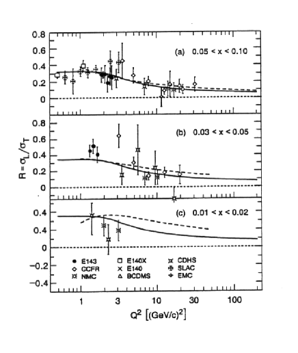
FIG. 2.: World compilation of R as a function of $Q^{2}$ for various small $x$ values, curves are a fit of E143 Collaboration[8] .

If one neglects the electron mass $m_{e}$, the cross section eq.(5) reads

$$\frac{d^{2}\sigma}{dE^{\prime}d\Omega_{e}}=\frac{4\alpha^{2}(E^{\prime})^{2}}{Q^{4}}\left[W_{2}\cos^{2}\theta/2+2W_{1}\sin^{2}\theta/2\right]\ ,$$ (10)

and for the elastic contribution when $Q^{2}=2M\nu$, i.e. $x=1$, we have with $\tau=Q^{2}/4M^{2}$,

$$W^{e\ell}_{1} = \tau G^{2}_{M}\delta(\nu-Q^{2}/2M)\ ,$$ (11)

$$W^{e\ell}_{2} = \frac{G^{2}_{E}+\tau G^{2}_{M}}{1+\tau}\delta(\nu-Q^{2}/2M)\ ,$$ (12)

where $G_{E}$ and $G_{M}$ are the electric and magnetic form factors. Clearly this contribution vanishes in the large $Q^{2}$ region since $G_{E,M}(Q^{2})\sim(Q^{2})^{-2}$ . However for a point-like particle, from eq.(12) we have

$$2MW_{1}^{pt}=x\delta(1-x)\quad\hbox{and}\quad\nu W_{2}^{pt}=\delta(1-x)\ ,$$ (13)

where $x=Q^{2}/2M\nu$, and we will come back later to this important result. From the 1968 SLAC experiment[1], it was observed that at a fixed value of $W^{2}$, the invariant square mass of $X$ (see eq.(2)), when $Q^{2}$ is large enough, both $MW_{1}$ and $\nu W_{2}$ vanish, like in the elastic case. However in the scaling limit, that is when both $\nu$ and $Q^{2}$ are large, with $x=Q^{2}/2M\nu$ fixed, this is no longer the case and according to Bjorken [2], one expects

$$MW_{1}(\nu,Q^{2})\mathrel{\mathop{\kern 0.0pt\longrightarrow}\limits_{Q^{2}\to\infty}}F_{1}(x)\ ,\qquad\nu W_{2}(\nu,Q^{2})\mathrel{\mathop{\kern 0.0pt\longrightarrow}\limits_{Q^{2}\to\infty}}F_{2}(x)\ ,$$ (14)

where $F_{1,2}(x)$ are two scaling functions independent of $Q^{2}$. Therefore the SLAC experiment has shown that the DIS cross section is much larger than expected and obeys scaling as predicted by Bjorken. These observations were the basis of the Feynman’s idea for the parton model which can be formulated as follows: hadrons possess a granular structure and the ”granules” behave as hard point-like almost free objects.

Finally we recall that the structure functions $W_{1}$ and $W_{2}$ can be related to the absorption cross sections for transverse and longitudinal virtual photons $\sigma_{T}$ and $\sigma_{L}$

$$W_{1}(\nu,Q^{2}) = \frac{\sqrt{Q^{2}+\nu^{2}}}{4\pi\alpha^{2}}\sigma_{T}\,$$ (15)

$$W_{2}(\nu,Q^{2}) = \frac{1}{4\pi\alpha^{2}}\frac{Q^{2}}{\sqrt{Q^{2}+\nu^{2}}}(\sigma_{T}+\sigma_{L})\ .$$ (16)

This allows to write eq.(8) as

$$\frac{d^{2}\sigma}{dE^{\prime}d\Omega_{e}}=\Gamma(\sigma_{T}+\varepsilon\sigma_{L})\ ,$$ (17)

where $\varepsilon$ and $\Gamma$ are kinematic factors

$$\varepsilon=\left[1+2\frac{Q^{2}+\nu^{2}}{Q^{2}}\tan^{2}\theta/2\right]^{-1}\quad\hbox{and}$$ (18)

$$\Gamma=\frac{\sqrt{Q^{2}+\nu^{2}}}{2\pi^{2}Q^{2}}\frac{E^{\prime}}{E}\frac{1}{1-\varepsilon}\ .$$ (19)

The positivity of $\sigma_{L}$, $\sigma_{T}$ leads to the inequalities

$$0\leq W_{1}\leq\left(1+\frac{\nu^{2}}{Q^{2}}\right)W_{2}\ .$$ (20)

One also defines a useful quantity, the ratio $R$ of longitudinal to transverse cross sections for polarized virtual photons on an unpolarized target

$$R=\sigma_{L}/\sigma_{T}=\frac{W_{2}(\nu,Q^{2})}{W_{1}(\nu,Q^{2})}\left(1+\frac{\nu^{2}}{Q^{2}}\right)-1\ .$$ (21)

In the limit of large $Q^{2}$, $\sigma_{L}$ vanishes, so $R=0$ and we have $2xMW_{1}=\nu W_{2}$, that is the so-called Callan-Gross relation[6]

$$2xF_{1}(x)=F_{2}(x)\ ,$$ (22)

which is approximately valid for finite $Q^{2}$. However at finite $Q^{2}$, quark transverse momentum effects generate non-zero values of $R$. These have been observed in the measurements made at SLAC[7, 8] showing that $R$ is slowly varying with $Q^{2}$ at fixed $x$. A recent world data compilation is depicted in Fig. 2.

Although the two scaling functions $F_{1,2}(x)$ were introduced above in the limit ${Q^{2}\to\infty}$, for finite $Q^{2}$ we have $F_{1,2}(x,Q^{2})$ which are $Q^{2}$ dependent because of scaling violations. These important aspects will be discussed in section 0.1.4, but meanwhile in order to complete our presentation of the data, we give in Fig. 3 a compilation of $F_{1,2}^{p}(x,Q^{2})$ for fixed proton target experiments (NMC, BCDMS, E665) and collider experiments at HERA-DESY (ZEUS, H1). Within this broad kinematic domain in $x$ and $Q^{2}$, the data exhibit indeed, a clear evidence for scaling violations.

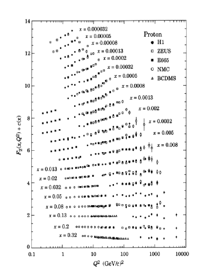
FIG. 3.: The structure function $F_{2}^{P}(x,Q^{2})$, data are from refs. [9, 10, 11, 12, 13]. For the purpose of plotting, a constant $c(x)=0.6(i_{x}-0.4)$ is added to $F_{1,2}^{p}(x,Q^{2})$, where $i_{x}$ is the number of the $x$ bin ranging from $i_{x}=1$ ($x=0.32$) to $i_{x}=21$ ($x=0.000032$) (Courtesy of R. Voss).

B The neutrino induced reactions $\nu(\bar{\nu})p\to\mu^{\mp}X$

For these reactions the proton is now probed by a weak charged current and the lowest order diagram is also shown in Fig. 1, where $\gamma^{\star}$ is replaced by a virtual $W^{\pm}$. Actually, if $\mu^{\pm}$ are replaced by $e^{\pm}$, one can also consider the line reversed reactions $e^{\mp}p\to\nu(\bar{\nu})X$ which will be studied at HERA DESY with polarized incident beams $e^{\mp}$. The cross section is in this case

$$\frac{d^{2}\sigma}{dE^{\prime}d\Omega}=\frac{G^{2}_{F}}{(2\pi)^{2}}\left(\frac{M^{2}_{W}}{M^{2}_{W}+Q^{2}}\right)^{2}\frac{E^{\prime}}{E}L^{(\nu)}_{\mu\nu}W^{\mu\nu}\ ,$$ (23)

with $G_{F}=10^{-5}/M^{2}$, $M_{W}=80.43\mbox{GeV}$ and where the leptonic tensor $L^{(\nu)}_{\mu\nu}$ is no longer symmetric

$$L^{(\nu)}_{\mu\nu}=k^{\prime}_{\mu}k_{\nu}+k_{\mu}k^{\prime}_{\nu}-k.k^{\prime}g_{\mu\nu}\pm i\varepsilon_{\mu\nu\rho\sigma}k^{\rho}k^{\prime\sigma}\ ,$$ (24)

with $+$ for the left-handed neutrino and $-$ for the right-handed antineutrino.

For the hadronic tensor associated to the weak charged current, which is not conserved, one has now in addition to the symmetric part analogous to the previous case, an antisymmetric term due to the interference between vector and axial parts of the current. The hadronic tensor can be expressed in terms of three structure functions

$$W_{\mu\nu} = W_{1}^{\nu}(\nu,Q^{2})\left(-g_{\mu\nu}+{\displaystyle\frac{q_{\mu}q_{\nu}}{q^{2}}}\right)$$ (28)

$$+{\displaystyle\frac{W^{\nu}_{2}(\nu,Q^{2})}{M^{2}}}\left(p_{\mu}-{\displaystyle\frac{p.q}{q^{2}}}q_{\mu}\right)\left(p_{\nu}-{\displaystyle\frac{p.q}{q^{2}}q_{\nu}}\right)$$

$$-{\displaystyle\frac{i}{M}}\varepsilon_{\mu\nu\rho\sigma}p^{\rho}q^{\sigma}W^{\nu}_{3}(\nu,Q^{2})\ .$$

The new structure function $W^{\nu}_{3}$, which is not necessarily positive, is due to the parity violating coupling of the weak gauge bosons $W^{\pm}$. The cross sections for $\nu$ and $\bar{\nu}$ now read

$$\frac{d^{2}\sigma^{\nu,\bar{\nu}}}{dE^{\prime}d\Omega}=\frac{G^{2}_{F}E^{\prime 2}}{2\pi^{2}(1+Q^{2}/M^{2}_{W})^{2}}\cdot$$ (29)

$$\left[W^{\nu}_{2}\cos^{2}\theta/2+2W^{\nu}_{1}\sin^{2}\theta/2\mp\left(\frac{E+E^{\prime}}{M}\right)W^{\nu}_{3}\sin^{2}\theta/2\right],$$ (30)

and clearly by taking the difference between $\nu$ and $\bar{\nu}$ cross sections one can isolate $W^{\nu}_{3}$. As in the previous case, one can interpret the $W^{\nu}_{i}(\nu,Q^{2})$ in terms of the virtual $W$-proton cross sections and from positivity one obtains the inequalities

$$0\leq\frac{\sqrt{Q^{2}+\nu^{2}}}{2M}|W^{\nu}_{3}|\leq W^{\nu}_{1}\leq(1+\nu^{2}/Q^{2})W^{\nu}_{2}\ .$$ (31)

Finally one also expects in the scaling limit

$$MW^{\nu}_{1}(\nu,Q^{2}) \mathrel{\mathop{\kern 0.0pt\rightarrow}\limits_{Q^{2}\to\infty}}F^{\nu}_{1}(x),$$ (32)

$$\nu W^{\nu}_{2}(\nu,Q^{2}) \mathrel{\mathop{\kern 0.0pt\longrightarrow}\limits_{Q^{2}\to\infty}}F^{\nu}_{2}(x),$$ (33)

$$\nu W^{\nu}_{3}(\nu,Q^{2}) \mathrel{\mathop{\kern 0.0pt\rightarrow}\limits_{Q^{2}\to\infty}}F^{\nu}_{3}(x),$$ (34)

where $F^{\nu}_{1,2,3}(x)$ are three scaling functions independent of $Q^{2}$ and similarly to eq.(22), one should have

$$2xF^{\nu}_{1}(x)=F^{\nu}_{2}(x)=x|F^{\nu}_{3}(x)|\ .$$ (35)

For finite $Q^{2}$ these three functions are also $Q^{2}$ dependent and for completness we show in Fig. 4, the results on $xF_{3}^{\nu N}$ from the CCFR collaboration [14] at FNAL, as a function of $Q^{2}$, for fixed $x$ values. The existence of scaling violations is also shown by these data.

FIG. 4.: The structure function $xF_{3}^{\nu N}(x,Q^{2})$, where $N$ stands for nucleon, versus $Q^{2}$ for different $x$ values. Data are from ref. [14] and for the purpose of plotting, a constant $c(x)=0.6(19-i_{x})$ is added to $xF_{3}^{\nu N}(x,Q^{2})$, where $i_{x}$ is the number of the $x$ bin ranging from $i_{x}=1$ ($x=0.0075$) to $i_{x}=18$ ($x=0.75$).

C $ep\to e^{\prime}X$ polarized case

Let us consider the case of DIS where both electron and proton are polarized. If $s_{e}$ denotes the polarization vector of the incident electron, it is a space-time vector orthogonal to the momentum $k$ of the electron, so it is such that $k.s_{e}=0$ and $s^{2}_{e}=-1$. Consequently the leptonic tensor $L_{\mu\nu}$ has now, in addition to the symmetric part (see eq.(6)), an antisymmetric part

$$L^{(A)}_{\mu\nu}=-2i\varepsilon_{\mu\nu\alpha\beta}s^{\alpha}_{e}q^{\beta}\ .$$ (36)

Similarly, if $s_{p}$ denotes the polarization vector of the proton the antisymmetric part of the hadronic tensor is linear in $s_{p}$ and reads

$$\kern-14.22636ptW^{(A)}_{\mu\nu} = i\varepsilon_{\mu\nu\alpha\beta}q^{\alpha}s^{\beta}_{p}MG_{1}(\nu,Q^{2})$$ (38)

$$+\frac{i\varepsilon_{\mu\nu\alpha\beta}}{M}q^{\alpha}\left[(p.q)s^{\beta}_{p}-(s_{p}.q)p^{\beta}\right]G_{2}(\nu,Q^{2})\ ,$$

where $G_{1,2}$ are two spin-dependent new structure functions. These structure functions can be related to the absorption cross sections $\sigma_{1/2}$ and $\sigma_{3/2}$ for virtual photons with projection $1/2$ and $3/2$ of the total spin along the incident photon direction. $\sigma_{T}$ introduced above (see eq.(16)) is the total transverse cross section $\sigma_{T}=\frac{1}{2}(\sigma_{1/2}+\sigma_{3/2})$ and $\sigma_{TL}$ is the cross section corresponding to the interference between the transverse and longitudinal polarizations of the photon. We have

$$\nu MG_{1}-Q^{2}G_{2} = \frac{\sqrt{Q^{2}+\nu^{2}}}{2\pi\alpha^{2}}(\sigma_{1/2}-\sigma_{3/2})\quad\hbox{and}$$ (39)

$$\sqrt{Q^{2}}(MG_{1}+\nu G_{2}) = \frac{\sqrt{Q^{2}+\nu^{2}}}{2\pi\alpha^{2}}\sigma_{TL}\ .$$ (40)

One can also define asymmetries for the virtual photon scattering, namely,

$$A_{1} = \frac{\sigma_{1/2}-\sigma_{3/2}}{\sigma_{1/2}+\sigma_{3/2}}=\frac{\nu MG_{1}-Q^{2}G_{2}}{W_{1}}\quad\hbox{and}$$ (41)

$$A_{2} = \frac{2\sigma_{TL}}{\sigma_{1/2}+\sigma_{3/2}}=\frac{\sqrt{Q^{2}}(MG_{1}+\nu G_{2})}{W_{1}}\ ,$$ (42)

with the following positivity bounds[15]

$$|A_{1}|\leq 1\quad\hbox{and}\quad|A_{2}|\leq\sqrt{R}\ ,$$ (43)

where $R$ is defined in eq.(21). The first inequality is rather trivial unlike the second one, which can badly restrict the allowed values of $A_{2}$. This bound has been recently improved [16] as follows

$$|A_{2}|\leq\sqrt{R(1+A_{1})/2}.$$ (44)

It involves $A_{1}$ and in the kinematic regions where $A_{1}$ is small or negative, one gets a much stronger bound than eq.(43) which corresponds to $A_{1}=1$. In the scaling limit one also expects

$$\nu M^{2}G_{1}(\nu,Q^{2}) \mathrel{\mathop{\kern 0.0pt\longrightarrow}\limits_{Q^{2}\to\infty}}g_{1}(x)\quad\hbox{and}$$ (45)

$$\nu^{2}MG_{2}(\nu,Q^{2}) \mathrel{\mathop{\kern 0.0pt\longrightarrow}\limits_{Q^{2}\to\infty}}g_{2}(x)\ ,$$ (46)

where $g_{1,2}(x)$ are two scaling functions independent of $Q^{2}$. Of course in this limit, $A_{2}$ is going to vanish since $R$ also goes to zero.

Finally these asymmetries $A_{1}$ and $A_{2}$ can be simply related to the measured spin asymmetries. In the case of longitudinal beam and target polarization along the beam direction (i.e. $s_{e}=\frac{1}{m_{e}}(|\vec{k}|,E\vec{k}/|\vec{k}|)$ and idem for $s_{p}$), one has

$$A_{\parallel}=\frac{d^{2}\sigma^{\uparrow\downarrow}-d^{2}\sigma^{\uparrow\uparrow}}{d^{2}\sigma^{\uparrow\downarrow}+d^{2}\sigma^{\uparrow\uparrow}}=D(A_{1}+\eta A_{2})\ ,$$ (47)

where $D$ and $\eta$ are kinematic factors (the factor $D$ is also called the depolarization factor)

$$D={1-E^{\prime}\varepsilon/E\over 1+\epsilon R},\quad\eta={\varepsilon\sqrt{Q^{2}}\over E-E^{\prime}\epsilon}\ .$$ (48)

In the region where $\nu$ and $Q^{2}$ are large, $\eta$ is small and one has

$$A_{\parallel}\sim DA_{1}\ .$$ (49)

In the case of longitudinally polarized beam and transversely polarized target (i.e. $s_{p}=(0,\vec{s})$, $\vec{s}.\vec{p}=0$ and $\vec{s}\ ^{2}=-1$), one has

$$A_{\perp}=\frac{d^{2}\sigma^{\uparrow\rightarrow}-d^{2}\sigma^{\uparrow\leftarrow}}{d^{2}\sigma^{\uparrow\rightarrow}+d^{2}\sigma^{\uparrow\leftarrow}}=d(A_{2}-\xi A_{1}),$$ (50)

where $d$ and $\xi$ are kinematic factors

$$d=D\sqrt{\frac{2\epsilon}{1+\epsilon}},\quad\xi=\eta{1+\epsilon\over 2\epsilon}\ .$$ (51)

When $\nu$ and $Q^{2}$ are large

$$A_{\perp}\sim dA_{2}\ .$$ (52)

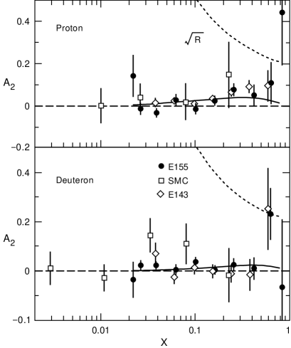
FIG. 5.: The world data on the asymmetries $A_{2}$ for proton and deuteron targets taken from ref.[17]. The weak positivity bound $\sqrt{R}$ is shown as the dotted curve. The solid curve was obtained by using $g_{2}$ given by the Wandzura-Wilczek sum rule. (see below eq.(86))

We show in Fig.5 a compilation of the world data on the asymmetries $A_{2}$ for polarized proton and deuteron targets, which turn out to be rather small. Experimental results on the asymmetry $A_{1}$ allow to extract the function $g_{1}$, which is also $Q^{2}$ dependent, and we show the most recent data at $Q^{2}=5GeV^{2}$, for a polarized proton target in Fig. 6 and for polarized deuterium and neutron targets in Fig. 7.

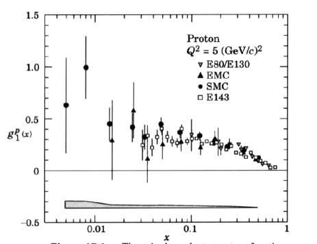
FIG. 6.: The world data on the structure functions $g_{1}^{p}(x)$ from experiments ref.[18, 19, 20, 21, 22].

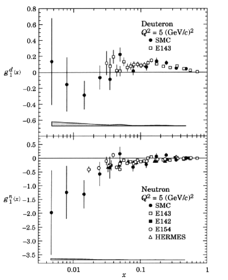
FIG. 7.: The world data on the structure functions $g_{1}^{d}(x)$ and $g_{1}^{n}(x)$ from various experiments ref. [23, 24, 25, 26, 27, 28].

III Physical interpretation of structure functions, parton distributions and sum rules

A The physical picture : the quark parton model

The experimental facts observed at SLAC in 1968[1] gave a strong support to the existence of point-like objects in the proton structure and were the inspiration for trying to elaborate a simple physical picture for interpreting the structure functions of DIS. When $E\to\infty$ (i.e. $\nu\to\infty$), because of time dilatation, the life time of the proton virtual states is also very large. When $Q^{2}\to\infty$, the interaction time $1/\sqrt{Q^{2}}$ becomes very small. So in the scaling limit, $\nu$ and $Q^{2}$ very large, the virtual photon $\gamma^{\star}$ (see Fig. 1) sees a ”frozen” state of quasi-real, quasi-free point like objects called partons.

FIG. 8.: The parton model handbag diagram showing the interaction of $\gamma^{\star}$ with the parton of momentum $k$.

According to the parton model, in this kinematical region, the proton behaves as a gas of free partons. In particular, it is very unlikely to recover a proton in the final state and this is why the elastic form factors $G_{E,M}$ vanish when $Q^{2}\to\infty$, as recalled above. So in the calculation of the DIS cross section (e.g. see eq.(5)), the hadronic tensor $W_{\mu\nu}$ is evaluated according to the parton model graph, shown in Fig. 8, namely

$$W_{\mu\nu}=\sum_{i}\sum_{s}\int d^{4}kf^{i}_{s}(p,k)w^{i}_{\mu\nu}(q,k)\delta[(k+q)^{2}],$$ (53)

where $f^{i}_{s}(p,k)$ is the probability for the virtual photon to struck a parton $i$ of spin $s$ and momentum $k$, inside the proton of momentum $p$. It seems very natural nowdays to assume that the charged partons which interact directly with $\gamma^{\star}$ are quarks. This step was not so obvious to make in 1968, although we had already the $SU(3)$ classification of hadrons, as built up from quarks, and the Cabibbo theory of weak interactions simply formulated in terms of leptons and quarks. It is important to recall that nowdays six quarks have been identified. They have very different masses: three of them are the light quarks up, down and strange ($u,d,s$) and three are the heavy quarks charm, bottom and top ($c,b,t$). The quark flavor corresponds to one of these six labels $u,d,s,c,b,t$ and the $u,c,t$ quarks have a charge $e=2/3$, while the charge of the $d,s,b$ quarks is $e=-1/3$. The summation over $i$ in eq.(53)) and subsequent equations stands for a flavor summation $i=u,d,s,..$. In the nucleon $u$ and $d$ quarks dominate and their mass can be neglected in high energy DIS. So if these partons are indeed spin $1/2$ massless quarks, we are now in the framework of the quark parton model (QPM), $w^{i}_{\mu\nu}(q,k)$ is the tensor which describes the interaction of $\gamma^{\star}$ with the quark $i$ of momentum $k$ and we have, for its symmetric part

$$w^{i}_{\mu\nu}(q,k)=\frac{e^{2}_{i}}{2}Tr\left\{\hbox to0.0pt{/\hss}k\gamma_{\mu}(\hbox to0.0pt{/\hss}k+\hbox to0.0pt{/\hss}q)\gamma_{\nu}\right\}\ ,$$ (54)

which is similar to the leptonic tensor (e.g. see eq.(6)). If $x_{i}$ is the fraction of the proton momentum carried by the quark $i$, $x_{i}=k.q/M\nu$, so $\delta[(k+q)^{2}]=\frac{1}{2M\nu}\delta(x-x_{i})$ and the hadronic tensor becomes

$$W_{\mu\nu} = \sum_{i}e^{2}_{i}\sum_{s}\frac{d^{4}k}{2M\nu}f^{i}_{s}(p,k)\delta(x-x_{i})\cdot$$ (56)

$$[2k_{\mu}k_{\nu}+k_{\mu}q_{\nu}+k_{\nu}q_{\mu}-g_{\mu\nu}k.q],$$

where $e_{i}$ is the charge of the quark $i$. From this expression, one can extract $W_{1,2}$ whose features correspond to the scattering of point-like objects (see eq.(13)) and by comparing with eq.(9), one finds after some partial integration and using eq.(14)

$$F_{1}(x)=\frac{1}{2}\sum_{i}e^{2}_{i}q_{i}(x)\ ,$$ (57)

where

$$q_{i}(x)=\sum_{s=\pm}\int d^{2}k_{T}f^{i}_{s}(p,k)=q_{i+}(x)+q_{i-}(x).$$ (58)

Clearly $q_{i}(x)$, which is called the unpolarized quark distribution function, contains the sum over two quark spin directions and the average over the quark intrinsic transverse momentum $k_{T}$. Usually in the QPM one interprets $q_{i+(-)}(x)dx$ as the probability to find a quark $i$, with helicity parallel (antiparallel) to the nucleon spin, and with momentum fraction of the proton between $x$ and $x+dx$. From eq.(56) one also finds $\nu W_{2}=2xMW_{1}$, that is the Callan-Gross relation (see eq.(22)) which leads to $R=0$, as mentioned before. This is what one expects for quarks of spin $1/2$ and let us recall the argument. Consider a collision quark-virtual photon in the Breit frame. By conservation of the total spin along the momentum direction, a scalar quark $(s=0)$ cannot absorb a photon of helicity $\lambda=\pm 1$, so $\sigma_{T}=0$ and $R=\infty$. However for $s=1/2$, the quark helicity flips in the electromagnetic interaction and therefore only the photon with $\lambda=\pm 1$ can be absorbed, so $\sigma_{L}=0$ and $R=0$.

Finally let us consider polarized DIS and the interpretation of the polarized structure functions $g_{1,2}(x)$. Similarly in the QPM, the antisymmetric part of the hadronic tensor (see eq.(38)) can be expressed as

$$W_{\mu\nu}^{(A)}\!\!=\!\!\sum_{i}\!\sum_{s}d^{4}kf^{i}_{s}(p,k,s_{p})w_{\mu\nu}^{(A)i}(q,k,s)\delta[(k+q)^{2}],$$ (59)

where $s_{p}$ denotes the proton polarization vector and

$$w_{\mu\nu}^{(A)i}=\frac{e^{2}_{i}}{4}Tr\left\{(1+\hbox to0.0pt{/\hss}s\gamma_{5})\hbox to0.0pt{/\hss}k\gamma_{\mu}(\hbox to0.0pt{/\hss}k+\hbox to0.0pt{/\hss}q)\gamma_{\nu}\right\}\ .$$ (60)

So

$$W_{\mu\nu}^{(A)} = i\varepsilon_{\mu\nu\rho\sigma}q_{\rho}\sum_{i}e^{2}_{i}\int d^{4}k\left[f^{i}_{+}(p,k,s_{p})-f^{i}_{-}(p,k,s_{p})\right]\cdot$$ (62)

$$k_{\sigma}\delta\left[(k+q)^{2}\right]\ .$$

By comparing with eq.(38) and using eq.(46) one finds

$$g_{1}(x)=\frac{1}{2}\sum_{i}e^{2}_{i}\Delta q_{i}(x)\quad\hbox{and}\quad g_{2}(x)=0\ ,$$ (63)

where with the help of the definitions in eq.(58)

$$\Delta q_{i}(x)=q_{i+}(x)-q_{i-}(x)\ ,$$ (64)

which is called the polarized quark distribution function. Therefore in the scaling limit the longitudinal polarization of the proton is described by $g_{1}(x)$ and we find that $g_{2}(x)$ vanishes.

Actually if one goes beyond the most naive QPM (see section IV), one must also consider the existence of gluons which produce quark-antiquark pairs. Since the antiquark contribution can be computed similarly, all the above quark distributions must be replaced by adding quarks and antiquarks, so the correct expressions are indeed

$$F_{1}(x)=\frac{1}{2}\sum_{i}e^{2}_{i}\left[q_{i}(x)+\bar{q}_{i}(x)\right]\quad\hbox{and}$$ (65)

$$g_{1}(x)=\frac{1}{2}\sum_{i}e^{2}_{i}\left[\Delta q_{i}(x)+\Delta\bar{q}_{i}(x)\right]\ .$$ (66)

One sees from these expressions that by measuring only $F_{1}(x)$ (or $F_{2}(x)$), it will not be possible to disentangle neither unpolarized quark distributions of different flavors, nor quarks from antiquarks. For polarized quark (antiquark) distributions the situation is the same if one measures only $g_{1}(x)$. So we give now a short discussion to clarify this point.

Let us go back to $\nu(\bar{\nu})p\to\mu^{\mp}X$ which are interpreted in the QPM in terms of four different scattering processes, i.e. $\nu q$, $\nu\bar{q}$, $\bar{\nu}q$ and $\bar{\nu}\bar{q}$. For $\nu q$ scattering (resp. $\bar{\nu}\bar{q}$) both $\nu$ and $q$ are left-handed (resp. both $\bar{\nu}$ and $\bar{q}$ are right-handed), so the cross section $d\sigma/dy$ is isotropic ($s$ wave) whereas for $\nu\bar{q}$ since $\bar{q}$ is right-handed, in this case ($p$ wave) $d\sigma/dy\sim\left(\frac{1+\cos\theta}{2}\right)^{2}\sim(1-y)^{2}$, (idem for $\bar{\nu}q$ since $q$ is left-handed). Therefore one can write for a given flavor

$$\frac{d^{2}\sigma^{\nu}}{dxdy}\sim\left[q(x)+(1-y)^{2}\bar{q}(x)\right]\quad\hbox{and}$$ (67)

$$\frac{d^{2}\sigma^{\bar{\nu}}}{dxdy}\sim\left[\bar{q}(x)+(1-y)^{2}q(x)\right]\ .$$ (68)

Consequently the $y$ dependence allows to separate $q(x)$ from $\bar{q}(x)$ and by measuring both $\nu$ and $\bar{\nu}$ cross sections, one can isolate $q(x)-\bar{q}(x)$ and therefore we have (see eqs.(29) and (33))

$$xF^{\nu}_{3}(x)=\sum_{i}x(q_{i}(x)-\bar{q}_{i}(x))\ .$$ (69)

A similar analysis can be done to separate $\Delta q(x)$ from $\Delta\bar{q}(x)$ by using charged current reactions in $e^{\pm}p$ polarized DIS, which might be done at HERA DESY in the future.

B Main features of quark distributions from DIS data

Once the parton structure of the proton has been detected, to establish it firmly, we need to make a detailed study of its basic constituents. A very high energy proton is not a simple three quarks objects like a proton at rest, but much more complex and it is actually made of valence quarks, gluons and quark-antiquark pairs which carry a small fraction of its momentum (see Fig. 9). We define the valence quark distributions as

$$q_{val}(x)=q(x)-\bar{q}(x)=q(x)-q_{sea}(x)\ ,$$ (70)

where $q_{sea}(x)$ denotes the sea quark distribution and we assume $q_{sea}(x)=\bar{q}(x)$. From neutrino-nucleon DIS via the charged current, one can extract valence quarks from the measurement of $F^{\nu}_{3}(x)$ (see eq.(69)) and the most accurate data comes from CCFR[14] shown in Fig. 4. By looking at a fixed $Q^{2}$ value, as shown in Fig. 11, we see from this pure valence

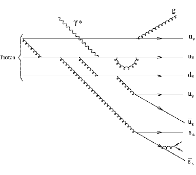
FIG. 9.: A microscopic view of the proton seen by a $\gamma^{*}$ having a large $Q^{2}$ and a large $\nu$.

contribution, that $xu_{val}(x)$ and $xd_{val}(x)$ are maximum around $x\sim 0.2$ or so and they vanish for $x\sim 1$ and $x\sim 0$. Since one can also isolate the antiquark distributions, the results from CCFR[14] show that $x\bar{q}(x)$ (or $xq_{sea}(x)$) goes to zero very rapidly for $x\sim 1$ and has a sharp rise for $x\sim 0$ (see Fig. 11). The small $x$ kinematic region which corresponds to $Q^{2}$ fixed and $\nu\to\infty$, is called the Regge region. A simple Regge analysis of the absorption cross sections $\gamma^{\star}p$ leads to

$$q_{sea}(x)\mathrel{\mathop{\kern 0.0pt\longrightarrow}\limits_{x\to 0}}1/x\quad\hbox{and}\quad q_{val}(x)\mathrel{\mathop{\kern 0.0pt\longrightarrow}\limits_{x\to 0}}1/\sqrt{x}\ .$$ (71)

Clearly the singular behavior shown in Fig.11 is stronger than this prediction and we will come back to this important point. From $ep\to e^{\prime}X$ and $ed\to e^{\prime}X$ DIS on hydrogen and deuterium targets, one can extract the electromagnetic structure functions $F^{p}_{2}(x)$ and $F^{n}_{2}(x)$ for proton and neutron, in terms of valence quark and antiquark distributions.

FIG. 10.: The structure function $xF_{3}^{\nu N}(x)$ versus $x$ at $Q^{2}=3GeV^{2}$ taken from ref.[14].

FIG. 11.: The antiquark distribution at $Q^{2}=3GeV^{2}$ (full circles) and $Q^{2}=5GeV^{2}$ (full triangles) versus $x$ taken from ref. [14].

By using eq.(22) and eq.(66) we have

$$F^{p}_{2}(x) = \frac{4}{9}\left[xu_{val}(x)+2x\bar{u}(x)\right]+\frac{1}{9}\left[xd_{val}(x)+2x\bar{d}(x)\right]$$ (73)

$$+\frac{1}{9}\left[xs(x)+x\bar{s}(x)\right]\ ,$$

if we restrict ourselves to three flavors $u,d$ and $s$. $F^{n}_{2}(x)$ is obtained from eq.(73) by exchanging $u$ and $d$. The NMC experiment at CERN[9] provides a rather accurate determination of $F^{n}_{2}(x)/F^{p}_{2}(x)$ and $F^{p}_{2}(x)-F^{n}_{2}(x)$ as shown in Fig.12. These data confirm and complete some of the features observed in neutrino data. The difference $F^{p}_{2}(x)-F^{n}_{2}(x)$ has a maximum around $x=0.3$ or so, where $u_{val}(x)$ and $d_{val}(x)$ dominate and it vanishes for $x\sim 1$. As we will see later, its behavior in the small $x$ region has revealed the flavor symmetry breaking of the sea quarks, i.e. $u_{sea}(x)\not=d_{sea}(x)$.

FIG. 12.: Ratio $F_{2}^{n}/F_{2}^{p}$ as a function of $x$ for differents $Q^{2}$ values, data are from NMC[29] and E665 [30]. Difference $F_{2}^{p}-F_{2}^{n}$ as a function of $x$ for $Q^{2}=4\mbox{GeV}^{2}$, data are from NMC[9].

Since sea quarks dominate for small $x$, we expect the ratio $F^{n}_{2}(x)/F^{p}_{2}(x)$ to go to one in the low $x$ region as indicated by the NMC data. The E665 data, which have larger errors, suggest a departure from this trend in the very small $x$ region. The behavior of $F^{n}_{2}(x)/F^{p}_{2}(x)$ for large $x$ indicates that $u_{val}(x)$ dominates over $d_{val}(x)$. The NuSea-experiment[31], has measured the ratio of muon pair yields from Drell-Yan production of proton-proton or proton-deuteron interactions. This ratio allows the determination of $\bar{d}/\bar{u}$ ratio (see Fig. 14), which has a strong $x$ dependence and confirms the antiquark flavor asymmetry, mentioned above and the fact that $\bar{d}>\bar{u}$. Using a parametrization of $\bar{d}+\bar{u}$, one can also extract $\bar{d}-\bar{u}$ (see Fig.14), which is mainly positive (except may be at large $x$) and exhibits a rapid rise for low $x$, in agreement with what was observed in neutrino DIS (see Fig. 11).

FIG. 13.: $\bar{d}$/$\bar{u}$ at $Q=7.35\mbox{GeV/c}$ measured by FNAL E866 experiment[31].

FIG. 14.: $\bar{d}-\bar{u}$ at $Q=7.35\mbox{GeV/c}$ extracted from FNAL E866 experiment [31].

The simple parametrization $\bar{d}(x)-\bar{u}(x)=(1-x)^{7}$, which was proposed ten years ago [32], is consistent with these new data (see Fig.14). The antiquark flavor asymmetry is an important topic which has generated new developments and for a complete review see ref.[33].

We have already said that a direct flavor decomposition of the polarized quark distributions is not possible from the data on $g^{p}_{1}(x)$ and $g^{d}_{1}(x)$ (see eq.(66)), but this can be done using polarized semi-inclusive DIS, where one detects a hadron in the final state. We show in Fig. 15 some recent results from HERMES [34] for the determination of $x\Delta u_{v}(x)$, which turns out to be positive, $x\Delta d_{v}(x)$ which is negative and $x\Delta\bar{u}(x)$ which is compatible with zero. The accuracy of these results is limited, but these trends agree with some global fits of the $g_{1}^{p,n,d}(x,Q^{2})$ data, as we will see later.

We now turn to a short review of different sum rules, the structure functions we have introduced so far must satisfy. We will also discuss their validity or breakdown versus experiment, as well as some theoretical considerations.

FIG. 15.: The polarized quark distributions at $Q^{2}=2.5GeV^{2}$ separately for the valence quarks $x\Delta u_{v}(x)$, $x\Delta d_{v}(x)$ and the sea quarks $x\Delta\bar{u}_{v}(x)$ as a function of $x$ (Taken from ref. [34]). The solid lines indicate the positivity limit and the dashed lines are a model parametrization.

C Sum rules

There exists a number of sum rules for unpolarized and polarized structure functions, some of which are rigorous results and other which rely on more or less well justified assumptions. Let us first consider the unpolarized case and for the electromagnetic structure functions we start with the Gottfried sum rule[35] (GSR). If one assumes an $SU(2)$ symmetric sea, i.e. $\bar{u}(x)=\bar{d}(x)$, one can easily show, using eq.(73), that

$$I_{G}=\int^{1}_{0}\frac{dx}{x}\left[F^{p}_{2}(x)-F^{n}_{2}(x)\right]=\frac{1}{3}\ ,$$ (74)

because

$$N_{u}=\int^{1}_{0}dx\ u_{val}(x)=2\quad\hbox{and}\quad N_{d}=\int^{1}_{0}dx\ d_{val}(x)=1\ .$$ (75)

In fact the NMC experiment[9] has observed a large defect of the GSR, since their measurement (see Fig. 12) gives at $Q^{2}=4\mbox{GeV}^{2}$, $I_{G}=0.235\pm 0.026$. This flavor symmetry breaking, more precisely $\bar{d}>\bar{u}$, is a consequence of the Pauli exclusion principle which favors $d\bar{d}$ pairs with respect to $u\bar{u}$ pairs, since the proton contains two $u$ quarks and only one $d$ quark.

Next for the charged current structure functions, we have two rigourous results based on eq.(75), namely the Adler sum rule[36] (ASR)

$$\int^{1}_{0}\frac{dx}{2x}\left[F^{\bar{\nu}p}_{2}(x)-F^{\nu p}_{2}(x)\right]=N_{u}-N_{d}=1\,$$ (76)

(an experimental verification[37] with large errors show an agreement) and the Gross-Llewellyn Smith sum rule[38] (GLSSR)

$$I_{GLS}\!\!=\!\!\int^{1}_{0}\frac{dx}{2x}\left[xF^{\nu p}_{3}(x)+xF^{\bar{\nu}p}_{3}(x)\right]\!\!=\!\!N_{u}+N_{d}\!=\!3.$$ (77)

The ASR is exact and receives no QCD corrections, but its experimental verification is at a very low level of accuracy [37]. The GLSSR gets a negative QCD correction and the CCFR data (see Fig.4) gives[14] $I_{GLS}=2.55\pm 0.06\pm 0.1$ at $Q^{2}=3\mbox{GeV}^{2}$, in fair agreement with the theoretical prediction. If we turn to polarized structure functions, there is first a fundamental result called the Bjorken sum rule[39] (BSR). It was derived about thirty years ago in the framework of quark current algebra and it relates the first moment of the difference between $g^{p}_{1}(x)$ for the proton and $g^{n}_{1}(x)$ for the neutron and the neutron $\beta$-decay axial coupling

$$\int^{1}_{0}dx\left[g^{p}_{1}(x)-g^{n}_{1}(x)\right]=\frac{1}{6}g_{A}/g_{V}\ ,$$ (78)

where $g_{A}/g_{V}=1.2573\pm 0.0028$ is very accurately known. The BSR gets also a negative QCD correction and we will come back later to the test of this firm prediction of QCD. One can also derive sum rules for $g^{p}_{1}$ and $g^{n}_{1}$ separately. These are the Ellis-Jaffe sum rules[40] (EJSR) which read

$$\Gamma_{1}^{p}=\int^{1}_{0}dxg^{p}_{1}(x)=\frac{1}{18}(9F-D+6\Delta s)\quad\hbox{and}$$ (79)

$$\Gamma_{1}^{n}=\int^{1}_{0}dxg^{n}_{1}(x)=\frac{1}{18}(6F-4D+6\Delta s)\ ,$$ (80)

where $F=0.459\pm 0.008$ and $D=0.798\pm 0.008$ are the $\beta$-decay axial coupling constants of the baryon octet and $\Delta s=\int^{1}_{0}\Delta s(x)dx$ is the total polarization of the proton carried by the strange quarks. One recovers eq.(78) by taking the difference because $F+D=g_{A}/g_{V}$. In their original work, Ellis and Jaffe made the critical assumption that $\Delta s=0$, which allows to make definite predictions for $\Gamma^{p}_{1}$ and $\Gamma^{n}_{1}$.

FIG. 16.: a) $I_{GDH}$ for proton, as a function of $Q^{2}$ for various upper limits of integration $W^{2}\leq 4.2\mbox{GeV}^{2}$ (triangles), $W^{2}\leq 45\mbox{GeV}^{2}$ (squares), the total integral (circles) from HERMES col.[42]. The curve is a theoretical prediction[43]. b) $I_{GDH}Q^{2}/(16\pi^{2}\alpha)$ as a function of $Q^{2}$ shows the weak $Q^{2}$-dependence of $\Gamma_{1}$.

Using the spin-dependent photoabsorption cross sections $\sigma_{1/2(3/2)}(\nu)$, Gerasimov-Drell-Hearn[41] (GDH) have derived the following sum rule valid for real photons

$$I_{GDH}=\int_{\nu_{thr}}^{\infty}[\sigma_{1/2}(\nu)-\sigma_{3/2}(\nu)]\frac{d\nu}{\nu}=-{2\pi^{2}\alpha\over M^{2}}\kappa^{2}\ ,$$ (81)

where $\nu$ is the photon energy in the target rest frame, $\nu_{thr}$ is the pion production threshold and $\kappa$ the anomalous nucleon magnetic moment. This important sum rule which predicts $-204\mu b$ for the proton, has never been tested directly due to the need for a circularly polarized beam with a longitudinally polarized target and a wide range of photon energies to be covered. However the GDH integral can be generalized to the case of absorption of polarized transverse virtual photons with $Q^{2}$

$$I_{GDH}(Q^{2})=\int_{\nu_{thr}}^{\infty}[\sigma_{1/2}(\nu,Q^{2})-\sigma_{3/2}(\nu,Q^{2})]\frac{d\nu}{\nu}.$$ (82)

One can show that, within a good approximation, one has in the scaling limit

$$I_{GDH}(Q^{2})=\frac{16\pi^{2}\alpha}{Q^{2}}\Gamma_{1}\,$$ (83)

where $\Gamma_{1}=\int^{1}_{0}dxg_{1}(x)$, so the GDH sum rule is connected to polarized DIS. The $Q^{2}$-dependence of the generalized GDH sum rule has been measured by the HERMES Collaboration[42] in the range $1.2\leq Q^{2}\leq 12\mbox{GeV}^{2}$ (see Fig.16). The $Q^{2}$-behavior of $I_{GDH}(Q^{2})$ agrees with the theoretical prediction of ref.[43] and this suggests that there are no important effects from either resonances or non-leading-twist.

Concerning the structure function $g_{2}(x)$, which is related to transverse polarization (see eq.(52), but has no simple interpretation in the parton model, it is possible to derive a superconvergence relation by considering the asymptotic behavior of a particular virtual Compton helicity amplitude. This leads to the Burkhardt-Cottingham sum rule[44] (BCSR)

$$\int^{1}_{0}dxg^{p}_{2}(x)=0\quad\hbox{and}\quad\int^{1}_{0}dxg^{n}_{2}(x)=0\ ,$$ (84)

for proton and neutron and from this result, it has been naively argued that $g_{2}(x)$ vanishes identically. Actually from what we discussed in section II about the asymmetry $A_{2}$ in the scaling limit, one can alternatively expect $g_{1}(x)+g_{2}(x)=0$, a simple relation between $g_{1}$ and $g_{2}$. However $g_{2}(x)$ is more complicated than that[45] and only part of it (twist-$2$ contribution) is entirely related to $g_{1}(x)$ by means of the Wandzura-Wilczek sum rule[46] (WWSR) which reads for $J\geq 1$

$$\int^{1}_{0}dxx^{J-1}\left[\frac{J-1}{J}g_{1}(x)+g^{WW}_{2}(x)\right]=0\ .$$ (85)

Clearly for $J=1$ one recovers the BCSR eq.(84) and for $J=2$ one has

$$g^{WW}_{2}(x)=\int^{1}_{x}g_{1}(y)\frac{dy}{y}-g_{1}(x)\ .$$ (86)

Very preliminary data obtained recently by E155X[47] and shown in Fig.17 for proton, are consistent with eq.(86), as shown by the dashed curves, but this has to wait for further confirmation. This approximation gives also the same kind of agreement with the $A_{2}$ data for proton and deuteron, as noticed above in Fig.5.

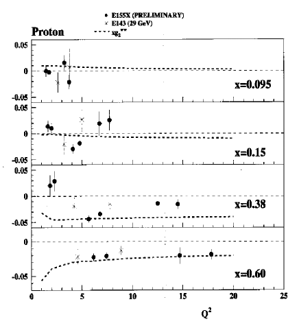
FIG. 17.: The structure function $xg^{p}_{2}$ versus $Q^{2}$ for different $x$ values. Preliminary data from SLAC E155X [47].

IV Beyond the QPM, scaling violations and phenomenological tests

A Scaling violations

So far we have considered the proton structure in the framework of the QPM, a picture valid only in the scaling limit. For finite $Q^{2}$, there are several experimental facts which confirm the existence of scaling violations and we have already shown in Figs. 3 and 4, the $Q^{2}$ dependence of $F_{2}^{p}(x,Q^{2})$ and $xF^{\nu N}_{3}(x,Q^{2})$, for different values of $x$. For small $x$, $F_{2}^{p}(x,Q^{2})$ increases with larger $Q^{2}$ and for large $x$, it decreases with larger $Q^{2}$. Actually this can be understood in the framework of QCD, a color gauge theory, which is the underlying field theory for describing quark interactions and in particular, deep inelastic phenomena.

From the knowledge of the structure functions $F^{p}_{2},F^{n}_{2},F^{\nu p}_{2}$ and $F^{\nu n}_{2}$, one basic observation, which was made long time ago, is the fact that in DIS, the total fraction of the proton momentum carried by quarks and antiquarks, i.e. $\sum_{j}\int^{1}_{0}dx\left[xq_{j}(x)+x\bar{q}_{j}(x)\right]$, is about $1/2$. So half of the proton momentum is carried by electrically neutral objects, which have been identified with the gluons, already mentioned above. Gluons are the carriers of the color force and therefore in the QPM diagram shown in Fig.8 (see also Fig.9), one can no longer neglect the possibility that the quark may radiate a gluon, before or after being struck by the virtual photon $\gamma^{\star}$. These contributions are of order $\alpha\alpha_{s}(Q^{2})$, where $\alpha_{s}(Q^{2})$ is the strong interaction coupling and moreover a gluon as a parton in the proton can contribute to DIS via the diagram $\gamma^{\star}g\to q\bar{q}$ to the same order. From the QCD Lagrangian and the corresponding Feynman rules one can compute these contributions, so partons in QCD[48] are no longer described by distributions which are functions of $x$ alone, but of $x$ as well as $Q^{2}$. These scaling violations will affect the predictions of the QPM and, as an example, the ratio $R$ (see eq.(21)) is not equal to zero, so the Callan-Gross relation (see eq.(22)) is not exact any more, and so on. The $Q^{2}$ dependence of the parton (quark, antiquark and gluon) distributions has been investigated by several authors[49] and can be summarized in the following way. Given the parton distributions at some reference point $Q^{2}=Q^{2}_{0}$, the $Q^{2}$ evolution is given by a set of coupled equations between singlet part $q^{S}=q+\bar{q}$ and gluon $G$

$$\frac{d}{d\ell nQ^{2}}\left(\begin{array}[]{c}q^{S}(x,Q^{2})\\ G(x,Q^{2})\end{array}\right)=\frac{\alpha_{s}(Q^{2})}{2\pi}\cdot$$ (89)

$$\int^{1}_{x}\frac{dz}{z}\left(\begin{array}[]{cc}P_{qq}(z)&N_{f}P_{qG}(z)\\ P_{Gq}(z)&P_{GG}(z)\end{array}\right)\left(\begin{array}[]{c}q^{S}(x/z,Q^{2})\\ G(x/z,Q^{2})\end{array}\right),$$ (94)

where $N_{f}$ is the number of flavors and the $P_{ij}(z)$, the so-called splitting functions, are known[48, 49]. This set of equations, usually called the DGLAP equations, is valid in leading order (LO) QCD, but it can be generalized to next-to-leading order (NLO), i.e. by including corrections of order $(\alpha_{s}(Q^{2}))^{2}$, because we have

$$P_{ij}(x)=P_{ij}^{(0)}(x)+\frac{\alpha_{s}}{2\pi}P_{ij}^{(1)}(x)+....$$ (95)

A more formal approach to derive the $Q^{2}$ behavior of the structure functions is based on the use of the operator product expansion[50] (OPE). The starting point is to consider time ordered products of two currents, which are related to the hadronic tensors introduced above, and to study their singularities on the light cone[51]. This is also a very powerful method to derive directly sum rules in QCD, together with their radiative corrections at the level of one or several loops.

Concerning the polarized distributions there exists a set of equations similar to eq.(94) which provides their $Q^{2}$ evolution[48], and the corresponding polarized splitting functions can be found in refs.[52, 53]. We note that in addition to the quark (antiquark) polarizations $\Delta q_{i}(x,Q^{2})$, one also introduces the gluon polarization $\Delta G(x,Q^{2})$ defined as in eq.(64). This distribution plays also a crucial rôle in connection with the anomaly of the axial current[54], as we briefly recall now[55]. For a given flavor $i$, the first moment $\Delta q_{i}$ is defined as the nucleon matrix element of the quark axial current

$$<p,s|\bar{q}_{i}\gamma_{\mu}\gamma_{5}q_{i}|p,s>=2s_{\mu}\Delta q_{i}\ .$$ (96)

Due to the fact that this axial current is not conserved, it was shown[54] that eq.(96) gets a gluon contribution which generates a shift of $\Delta q_{i}$

$$\Delta q_{i}\to\Delta q_{i}-\frac{\alpha_{s}(Q^{2})}{2\pi}\Delta G(Q^{2})\ .$$ (97)

It is worth recalling that from the QCD evolution equations $\Delta q_{i}$ is $Q^{2}$ independent, whereas $\Delta G(Q^{2})$ increases logarithmically with $Q^{2}$, but such an increase exactly compensates the decrease of $\alpha_{s}(Q^{2})$ with $Q^{2}$. However the size of this gluonic correction, which can be partly absorbed in the definition of the quark distributions, is purely a matter of scheme convention [56]. Finally we note that so far, we have no direct experimental information on the sign and magnitude of $\Delta G$.

B Phenomenological tests

There is an enormous literature devoted to phenomenological work on DIS but we shall discuss only very briefly, a few aspects of this broad area of high energy physics. Clearly one particular goal is to parametrize all the parton distributions as function of $x$, at a given low $Q^{2}$ value, $Q^{2}=Q_{0}^{2}$, and to test whether the $Q^{2}$ evolution agrees with the QCD predictions. In several analysis[57] the quark and gluon parton densities were described by a polynomial standard form

$$xp(x,Q^{2}_{0})=\eta Ax^{a}(1-x)^{b}(1+\gamma x+\rho\sqrt{x})\ ,$$ (98)

where $\eta,a,b,\gamma,\rho$ are free parameters. These twenty or so parameters were determined by making a global NLO fit of the data on unpolarized structure functions and the results obtained are rather satisfactory.

In a different approach, one is using, for valence quarks and antiquarks, a set of Fermi-Dirac distributions[58], with the following expression

$$xp(x,Q^{2}_{0})={Ax^{a}\over\exp[(x-V(x))/\bar{x}]+1}\ ,$$ (99)

where $V(x)$ plays the role of the ”thermodynamical potential” and $\bar{x}$ is the ”temperature”. The gluon density function $G(x,Q^{2}_{0})$ is given in this approach by a Bose-Einstein distribution with no free parameter.

In this case we have a small number of parameters, say ten at most, which were determined at $Q^{2}=4\mbox{GeV}^{2}$ by fitting the CCFR data displayed in Fig. 11 for valence quarks, in Fig. 11 for antiquarks and the NMC data on the ratio and the difference of $F^{p}_{2}$ and $F^{n}_{2}$ in Fig. 12.

FIG. 18.: Typical unpolarized parton density functions obtained from ref.[58].

FIG. 19.: Typical polarized parton density functions obtained from ref.[58].

From these distributions at $Q^{2}=4\mbox{GeV}^{2}$, after a standard $Q^{2}$ evolution using the DGLAP equations at LO only , one obtains the unpolarized parton distributions for different flavors, shown in Fig. 19 at $Q^{2}=20\mbox{GeV}^{2}$. We note that, as expected $u$ quarks dominate over $d$ quarks, $\bar{d}(x)>\bar{u}(x)$ and the $s$ and $c$ quarks are very small. Clearly the gluon distribution $G(x,Q^{2})$, which was divided by a factor 10 and represented by the curve $g/10$ in the Figure, dominates largely in the small $x$ region. The predictions obtained in a larger $Q^{2}$ range are in excellent agreement with the CCFR data for $xF_{3}^{\nu N}(x,Q^{2})$ depicted in Fig. 4 and also with the very recent data at HERA-DESY from the Zeus and H1 collaborations[10, 11] on $F_{2}^{p}(x,Q^{2})$ displayed in Fig. 3. The rapid rise in the very small $x$ region, down to $x=10^{-6}$ or so, where sea quarks dominate, is well described by the QCD predictions and this rise is the direct extrapolation of what has been observed by CCFR for $x=10^{-2}$. We gave only these two examples for illustration, but these tests have been widely extended as discussed in ref.[58]. The large amount of available data on the unpolarized structure functions was also used to perform a global analysis by several authors[57] and they all find for the parton densities a general pattern similar to the one displayed in Fig. 19.

We now turn to some tests involving the polarized structure functions. As we have seen before, there is a substantial experimental information on the $x$ dependence of $g_{1}^{p,n}(x)$ with proton, deuterium and ${}^{3}He$ polarized targets, for $Q^{2}$ in a rather limited range, i.e. $2\leq Q^{2}\leq 10\mbox{GeV}^{2}$. Given the present accuracy of the data and the small $Q^{2}$ range investigated so far, the $Q^{2}$ evolution of $g_{1}^{p,n}(x,Q^{2})$ predicted by QCD cannot be tested at the level it was done for the unpolarized case. Moreover this test depends on $\Delta G(x,Q^{2})$, for which only theoretical speculations can be made. In ref.[58], since the initial quark (antiquark) distributions are $q_{i\pm}(x,Q^{2})$ for each flavor $i$, one gets immediately $\Delta q_{i}(x,Q^{2})$. Therefore one can calculate consistently the $F_{2}$’s and the $g_{1}$’s structure functions, with no additional parameters and the agreement with the data is rather good[58]. We show in Fig. 19 a typical pattern of polarized parton distributions. $\Delta u(x)$ and $\Delta d(x)$ are rather well determined and they are consistent with the results shown in Fig. 15. We also see that $\Delta\bar{u}(x)$ is small and we find that $\Delta\bar{q}(x)$, for $q=d,s,c$ are compatible with zero. The $\Delta G(x)$ shown in the Figure is one possible solution but it has large uncertainties. There are several other QCD analysis of the $g_{1}$’s[59], where one relates the polarized parton distributions to the unpolarized ones with some additional parameters. These analysis conclude that $\Delta G$ is weakly constrained by present data and they all agree that a small $\Delta G$ is prefered.

Finally let’s say a few words on testing the first moment of $g_{1}$, i.e. the EJSR and the BSR. Since data are obtained for each $x$ at a different $Q^{2}$, in order to have $g_{1}(x,Q^{2})$ for a constant $Q^{2}$, one has to rely on the crucial hypothesis that the asymmetry $A_{1}$ (see eq.(42)) is $Q^{2}$ independent, so the $Q^{2}$ evolution of $g_{1}$ is driven by that of $F_{2}$.

Moreover, the sum rules involve integrals from $x=0$ to $x=1$ and since there is no data at both ends, one has to make some reliable extrapolations in these two regions, low $x$ being the most critical one. The QPM results given in eqs.(78) and (80) are modified by QCD corrections, which have been calculated up to order $(\alpha_{s}(Q^{2}))^{3}$. For example, in the gauge invariant factorization scheme, perturbative QCD corrections to $\Gamma_{1}^{p(n)}$ lead to the following results[60] :

$$\Gamma_{1}^{p(n)}=\,C_{NS}\left(\pm{1\over 12}g_{A}^{3}+{1\over 36}g_{A}^{8}\right)+{1\over 9}\,C_{S}g_{A}^{0},$$ (100)

where

$$g_{A}^{0} = \Delta\Sigma\equiv\Delta u+\Delta d+\Delta s,$$ (101)

$$g_{A}^{3} = F+D,$$ (102)

$$g_{A}^{8} = 3F-D,$$ (103)

the coefficients non-singlet $C_{NS}$ and singlet $C_{S}$ are given by

$$C_{NS} = 1-{\alpha_{s}\over\pi}-{43\over 12}\left({\alpha_{s}\over\pi}\right)^{2}-20.2153\left({\alpha_{s}\over\pi}\right)^{3},$$ (104)

$$C_{S} = 1-{\alpha_{s}\over\pi}-1.10\left({\alpha_{s}\over\pi}\right)^{2},$$ (105)

for three quarks flavors. The BSR becomes now

$$\Gamma_{1}^{p}-\!\Gamma_{1}^{n}=\frac{1}{6}\frac{g_{A}}{g_{V}}\left[1-\!\frac{\alpha_{s}}{\pi}-{43\over 12}\!\biggl{(}\frac{\alpha_{s}}{\pi}\biggr{)}^{2}-20.2153\!\biggl{(}\frac{\alpha_{s}}{\pi}\biggr{)}^{3}\right].$$ (106)

Here we have neglected the theoretical uncertainties in the very low $Q^{2}$ region due to the higher-twist effects which go like $1/Q^{2}$.

The world data for the $\Gamma_{1}(Q^{2})$’s show a defect in the EJSR for proton and deuterium both at $Q^{2}=3\mbox{GeV}^{2}$ from E143[22, 23] and $Q^{2}=10\mbox{GeV}^{2}$ from SMC[19, 25]. From this one deduces also a defect for neutron, which was confirmed by the E154 result. If one combines the world data one finds for the BSR

$$\Gamma_{1}^{p}-\Gamma_{1}^{n}=0.171\pm 0.005\pm 0.01\quad\mbox{at}\quad Q^{2}=5\mbox{GeV}^{2}\ ,$$ (107)

to be compared to the QCD prediction $0.182\pm 0.005$. One can also turn the argument around and given the experimental result, use the theoretical expression for the BSR to extract $\alpha_{s}(Q^{2})$[61]. We also note that the defect in $\Gamma_{1}^{p}$ and $\Gamma_{1}^{n}$ are usually interpreted as being mainly due to a large and negative $\Delta s$ (see eq.(80)), i.e. $\Delta s=-0.13\pm 0.02$, but of course this does not necessarily holds if one considers $SU(3)$ symmetry breaking effects[62]. The total contribution of the quark spins to the proton spin, is defined as $\Delta\Sigma=\Delta u+\Delta d+\Delta s$. For $\Delta s=0$, the Ellis-Jaffe[40] prediction gives $\Delta\Sigma\simeq 0.58$, but according to all experiments, one gets a smaller value, for instance, E155 experiment[27] has obtained $\Delta\Sigma=0.23\pm 0.04\pm 0.6$ at $Q^{2}=5\mbox{GeV}^{2}$, which is not so easy to reconcile with our first intuition from the naive quark model, namely, $\Delta\Sigma=1$.

V Summary

Our knowledge of the unpolarized and polarized structure functions has improved considerably over the last twenty years or so and consequently also, our basic understanding of the proton structure. The enormous quantity of high statistics experimental data which is now available, allows us to make rather precise tests of the QCD parton model and this theoretical picture is nowdays established on very serious basis. Deep inelastic phenomena is only one of the several areas of high energy particle physics which are the testing grounds of perturbative QCD and obviously, it has to be supplemented at least by electron-positron annihilation and hard hadron-hadron collisions[63].

For the unpolarized parton distributions, the flavor symmetry breaking of the sea quarks (i.e. $d_{sea}>u_{sea}$) was only discovered recently with the violation of the GSR and it should be investigated more precisely for example in Drell-Yan lepton pair production or in $W^{\pm}$ production[58]. Our knowledge about the gluon distribution, i.e. its small $x$ behavior and $Q^{2}$ dependence, is improving but a real experimental effort remains to be done to put it on equal footing with the quark distributions. It requires, for example, better measurements of $F_{2}^{p}(x,Q^{2})$ in the very small $x$ region and this makes HERA-DESY really exciting for the coming years.

Concerning the polarized parton distributions significant progress have been made and we have now the following results. The violation of the EJSR is confirmed for the proton and for the neutron. The BSR is verified up to 10% and this important test must be strengthened at a higher level of accuracy. The kinematic domain presently accessible is still too limited to answer some important questions, in particular about the small $x$ behavior of $g_{1}$, the $Q^{2}$ evolution of the quark distributions and about the, so far, elusive $\Delta G(x,Q^{2})$. The perspective of having polarized protons at HERA-DESY, which is seriously envisaged[64], is opening a new experimental window for answering these questions. Finally let us mention the very exciting spin physics programme which has been approved at RHIC-BNL and will start operating by 2001 as a polarized $pp$ collider[65]. Hopefully it will also shade some light on parton helicity distributions as well as quark transversity distributions. A facility called eRHIC, which combines a few GeV polarized electron beam onto one of the high energy polarized proton beam, is also under serious studies at BNL.

REFERENCES

- [1] W. K. H. Panofsky 1968, rapporteur talk, Proceedings of the 14th International Conference on High Energy Physics, Vienna, p.23 (Editors J. Prentki and J. Steinberger, CERN Geneva).
- [2] J. D. Bjorken 1969 Phys. Rev. 179, 1547.
- [3] R. P. Feynman 1969 Phys. Rev. Lett. 23, 1415.
- [4] H. D. Politzer 1974 Phys. Reports C14, 129.
- [5] A Collaboration, M. K. Jones et al. 2000 Phys. Rev. Lett. 84, 1398 and references therein.
- [6] C. G. Callan and D. G. Gross 1969 Phys. Rev. Lett. 22, 156.
- [7] L. W. Whitlow et al. 1990 Phys. Lett.B 250, 193.
- [8] SLAC E143, K. Abe et al. 1999 Phys. Lett. B452, 194.
- [9] New Muon Collaboration, M. Arneodo et al. 1994 Phys. Rev. D50, R1 and references therein; 1995 Phys. Lett. B364, 107.
- [10] ZEUS Collaboration, M. Derrick et al. 1995 Z. Phys. C65, 379; 1996 ibidem C72, 399; J. Breitweg et al. 1997 Phys. Lett. B407, 432.
- [11] H1 Collaboration, T. Ahmed et al. 1995 Nucl. Phys. B439, 471; S. Aid et al. 1996 ibidem B470, 3; C. Adloff et al. 1997 ibidem B497 3.
- [12] BCDMS Collaboration, A. C. Benvenuti et al. 1989 Phys. Lett. B223, 485.
- [13] FNAL E665 Collaboration, M. R. Adams et al. 1996 Phys. Rev. D54, 3006.
- [14] CCFR Collaboration, P. Z. Quintas et al. 1993 Phys. Rev. Lett. 71, 1307; W. C. Leung et al. 1993 Phys. Lett. B317, 655; J. H. Kim et al. 1998 Phys. Rev. Lett. 81, 3595.
- [15] M. G. Doncel and E. de Rafael 1971 Nuovo Cimento 4A, 363.
- [16] J. Soffer and O. V. Teryaev 2000 Phys. Lett. B490, 106.
- [17] SLAC E155 Collaboration, P.L. Anthony et al. 1999 Phys. Lett. B458, 529.
- [18] EMC Collaboration, J. Ashman et al. 1989 Nucl. Phys. B328, 1.
- [19] Spin Muon Collaboration, D. Adams et al. 1994 Phys. Lett. B329, 339; Erratum, 1994 Phys. Lett. B339, 332; 1997 ibidem B396, 338; B. Adeva et al. 1997 Phys. Lett. B412, 414.
- [20] SLAC E80 Collaboration, M. J. Alguard et al. 1976 Phys. Lett. 37, 1261; 1978 ibidem 41, 70.
- [21] SLAC E130 Collaboration, G. Baum et al. 1983 Phys. Rev. Lett. 51, 1135.
- [22] SLAC E143, K. Abe et al. 1995 Phys. Rev. Lett. 74, 346.
- [23] SLAC E143, K. Abe et al. 1995 Phys. Rev. Lett. 75, 25; 1998 Phys. Rev. D58, 112003.
- [24] SLAC E142, P. L. Anthony et al. 1993 Phys. Rev. Lett. 71, 959; 1996 Phys. Rev. D54, 6620.
- [25] Spin Muon Collaboration, D. Adams et al. 1995 Phys. Lett. B357, 248; 1997 Phys. Rev. D56, 5330; B. Adeva et al. 1998 Phys. Rev. D58, 112001.
- [26] SLAC E154 Collaboration, K. Abe et al. 1997 Phys. Lett. B405, 180.
- [27] SLAC E155 Collaboration, P. L. Antony et al. 2000 SLAC-PUB-7994 (hep-ph/0007248).
- [28] HERMES Collaboration, K. Ackerstaff et al. 1997 Phys. Lett. B404, 383; A. Airapetian et al. 1998 Phys. Lett. B442, 484.
- [29] P. Amaudruz et al. 1995 Nucl. Phys. B371, 3.
- [30] D. Adams et al. 1995 Phys. Rev. Lett. 75, 1466.
- [31] FNAL Nusea Collaboration, E. A. Hawker et al. 1998 Phys. Rev. Lett. 80, 3715; J. C. Peng et al. 1998 Phys. Rev. D58, 092004.
- [32] G. Preparata, P.G. Ratcliffe and J. Soffer 1991 Phys. Rev. Lett. 66, 687.
- [33] S. Kumano 1998 Phys. Rep. 303, 183.
- [34] HERMES Collaboration, K. Ackerstaff et al. 1999 Phys. Lett. B464, 123.
- [35] K. Gottfried 1967 Phys. Rev. Lett. 18, 1154.
- [36] S. L. Adler 1966 Phys. Rev. 143, 1144.
- [37] WA25 Collaboration, D. Allasia et al. 1985 Z. Phys C28 321.
- [38] D. Gross and C. Llewellyn Smith 1969 Nucl. Phys. B14, 337.
- [39] J. D. Bjorken 1966 Phys. Rev. 148, 1467 and 1970 ibid D1, 1376.
- [40] J. Ellis and R. Jaffe 1974 Phys. Rev. D9, 1444; 1974 D10 1669 (E).
- [41] S. B. Gerasimov 1966 Sov. J. Nucl. Phys. 2, 430; S. D. Drell and A. C. Hearn 1966 Phys. Rev. Lett. 16, 908.
- [42] HERMES Collaboration, A. Airapetian et al. 2000 Phys. Lett. B494, 1.
- [43] J. Soffer and O. V. Teryaev 1995 Phys. Rev. D51, 25.
- [44] H. Burkhardt and W. N. Cottingham 1970 Ann. Phys. 56, 453.
- [45] X. Ji 1995 Contribution to the Workshop on Deep Inelastic Scattering and QCD, Paris April 24-28, p. 435 (Editors J. F. Laporte and Y. Sirois).
- [46] S. Wandzura and F. Wilczek 1977 Phys. Lett. B 72, 195.
- [47] SLAC E155X Collaboration, contribution to the workshop on the Nucleon Structure in High x-Bjorken Region, P. Bosted et al. 2000, Philadelphia (USA), March 2000.
- [48] G. Altarelli 1982 Phys. Rep. C81, 1.
- [49] V. N. Gribov and L. N. Lipatov 1972 Sov. J. Nucl. Phys. 15, 438,675; G. Altarelli and G. Parisi 1977 Nucl. Phys. B126, 298; Yu. L. Dokshitzer 1977 Sov. J. JETP 46, 641.
- [50] K. G. Wilson 1969 Phys. Rev. 179, 1499.
- [51] R. A. Brandt and G. Preparata 1971 Nucl. Phys. B27, 541.
- [52] W. Vogelsang 1996 Nuc. Phys. B475, 47; 1996 Phys. Rev. D54, 2023.
- [53] R. Mertig and W. L. van Neerven 1996 Z. Phys C70 637 and references therein.
- [54] G. Altarelli and G. G. Ross 1988 Phys. Lett. B212, 391; R. D. Carlitz, J. C. Collins and A. H. Mueller 1988 Phys. Lett. 214, 229; A. V. Efremov and O. V. Teryaev 1988 JINR Report E2-88-287 unpublished.
- [55] For a more complete discussion on this and on many other aspects of polarized DIS see M. Anselmino, A. V. Efremov and E. Leader, 1995 Phys. Rep. 261, 1; B. Lampe and E. Reya, 2000 Phys. Rep. 332, 1.
- [56] For an extensive review on the issue of factorization schemes see H.Y. Cheng 1996, Int. J. Mod. Phys. A 11, 5109.
- [57] A. D. Martin, R. G. Roberts and W. J. Stirling 1994 Phys. Rev. D50, 6734; A. D. Martin, R. G. Roberts, W. J. Stirling and R. S. Thorne 1998 Eur. Phys. J. C4 463 and references therein; CTEQ Collaboration, J. Botts et al. 1993 Phys. Lett. B304, 159; H. L. Lai et al. 2000 Eur. Phys. J. C12, 375; M. Glück, E. Reya, M. Stratmann and W. Vogelsang, 1996 Phys. Rev. D53, 4775; T. Gehrmann and W. J. Stirling 1996 Phys. Rev. D53, 6100.
- [58] C. Bourrely and J. Soffer 1995 Nucl. Phys. B445, 341.
- [59] T. Gehrmann and W. J. Stirling 1995 Z. Phys. C65, 461; R. D. Ball, S. Forte and G. Ridolfi 1995 Nucl. Phys. B444, 287; F. Buccella, O. Pisanti, P. Santorelli and J.Soffer 1996 Nuovo Cim. A109 159; C. Bourrely, F. Buccella, O. Pisanti, P. Santorelli and J.Soffer 1998 Prog. Theo. Phys. 99, 1017; D. de Florian, O. Sampayo and R. Sassot, 1998 Phys. Rev. D 57, 5803; E. Leader, A. V. Sidorov and D.B. Stamenov 1998 Phys. Rev. D 58, 114028; Y. Goto et al. 2000 Phys. Rev. D 62, 034017; M. Botje 2000 Eur. Phys. J C 14 285.
- [60] S. A. Larin and J. A. M. Vermaseren 1991 Phys. Lett. B259, 345; S. A. Larin 1994 Phys. Lett. B334, 192 and references therein.
- [61] J. Ellis and M. Karliner 1995 Phys. Lett. B341, 397; Workshop on the prospects of spin physics at HERA, Desy-Zeuthen, August 28-31, 1995 (Editors J. Bluemlein and W. D. Nowak) DESY-95-2000, p. 3; G. Altarelli, R. D. Ball, S. Forte and G. Ridolfi 1997 Nucl. Phys. B496, 337.
- [62] J. Lichtenstadt and H. J. Lipkin 1995 Phys. Lett. B353, 119; B. Ehrnsperger and A. Schäfer 1995 Phys. Lett. B348, 619.
- [63] G. Sterman et al. 1995 Rev. Mod. Phys. 67, 157.
- [64] Proceedings of the Workshop on the prospects of spin physics at HERA, Desy-Zeuthen, August 28-31, 1995 (Editors J. Bluemlein and W. D. Nowak) DESY-95-2000. Proceedings of the Workshop on ”Polarized Protons at High Energies - Accelerator Challenges and Physics Opportunities”, DESY Hamburg, May 17-20, 1999 ( Editors A. De Roeck, D. Barber, G. Raedel).
- [65] N. Saito, invited talk at the 14th Int. Spin Physics Symposium, SPIN2000, Oct. 16-21, Osaka, Japan, to be published in the Proceedings.